A determination of $\left\langle A_{\mu}^{2}\right\rangle$ and the non-perturbative vacuum energy of Yang-Mills theory in the Landau gauge

Abstract

We discuss the 2-point-particle-irreducible $(2PPI)$ expansion, which sums bubble graphs to all orders, in the context of $SU(N)$ Yang-Mills theory in the Landau gauge. Using the method we investigate the possible existence of a gluon condensate of mass dimension two, $\left\langle A_{\mu}^{a}A_{\mu}^{a}\right\rangle$, and the corresponding non-zero vacuum energy. This condensate gives rise to a dynamically generated mass for the gluon.

LTH–569

1 Introduction.

Recently there has been growing evidence for the existence of a condensate of mass dimension two in $SU(N)$ Yang-Mills theory with $N$ colours. An obvious candidate for such a condensate is $\left\langle A^{a}_{\mu}A^{a}_{\mu}\right\rangle$. The phenomenological background of this type of condensate can be found in [1, 2, 3]. However, if one first considers simpler models such as massless $\lambda\phi^{4}$ theory or the Gross-Neveu model [4] and the role played by their quartic interaction in the formation of a (local) composite quadratic condensate and the consequent dynamical mass generation for the originally massless fields [4, 5, 6], it is clear that the possibility exists that the quartic gluon interaction gives rise to a quadratic composite operator condensate in Yang Mills theory and hence a dynamical mass for the gluons. The formation of such a dynamical mass is strongly correlated to a lower value of the vacuum energy. In other words the causal perturbative Yang Mills vacuum is unstable. From this viewpoint, mass generation in connection with gluon pairing has already been discussed a long time ago in, for example, [7, 8, 9, 10]. There the analogy with the BCS superconductor and its gap equation was examined. It was shown that the zero vacuum is tachyonic in nature and the gluons achieve a mass due to a non-trivial solution of the gap equation. Moreover, recent work using lattice regularized Yang Mills theory has indicated the existence of a non-zero condensate, $\left\langle A^{a}_{\mu}A^{a}_{\mu}\right\rangle$, [11]. There the authors invoked the operator product expansion, (OPE), on the gluon propagator as well as on the effective coupling $\alpha_{s}$ in the Landau gauge. Their work was based on the perception that, even in the relatively high energy region ($\sim 10$GeV), a discrepancy existed between the expected perturbative behaviour and the lattice results. It was shown that, within the momentum range accessible to the OPE, that this discrepancy could be solved with a $1/q^{2}$ power correction. They concluded that a non-vanishing dimension two condensate must exist. Further, the results of [12] give some evidence that instantons might be the mechanism behind the low-momentum contribution to condensate. As has been argued in [3], only the low-momentum content of the squared vector potential is accessible with the OPE. Moreover, they argue that there are also short-distance non-perturbative contributions to $\left\langle A_{\mu}^{2}\right\rangle$.

It is no coincidence the Landau gauge is used for the search for a dimension two condensate. Naively, the operator $A_{\mu}^{2}$ is not gauge-invariant. Although this does not prevent the condensate $\left\langle A_{\mu}^{2}\right\rangle$ showing up in gauge variant quantities like the gluon propagator, we should instead consider the gauge-invariant operator $(VT)^{-1}\min_{U}\int\left.d^{4}x\left(A_{\mu}^{U}\right)^{2}\right.$, where $VT$ is the space-time volume and $U$ is an arbitrary gauge transformation in order to assign some physical meaning to the operator. Clearly from its structure this operator is non-local and thus is difficult to handle. However, when we impose the Landau gauge, it reduces to the local operator $A_{\mu}^{2}$. Moreover, it has been shown that $\left\langle A_{\mu}^{2}\right\rangle$ is (on-shell) BRST invariant [14, 15, 16, 17]. Another motivation for studying $\left\langle A_{\mu}^{2}\right\rangle$ is the perceived connection between the gluon propagator and confinement. (See [18] and references therein.) More precisely, the gluon propagator exhibits an infrared suppression, as has been reported in many lattice simulations, [19, 20, 21] and using the Schwinger-Dyson approach, [22, 23, 24]. A dynamical gluon mass might serve as an indication for such a suppression. An attempt has already been made to explain confinement by a dual Ginzburg-Landau model or an effective string theory, in the Landau gauge, with the help of $\left\langle A_{\mu}^{2}\right\rangle$ [25]. The fact that $\left\langle A_{\mu}^{2}\right\rangle$ might be central to confinement, is supported by the observation that it undergoes a phase transition due to the monopole condensation in three dimensional compact QED [2, 3].

From these various analyses the importance of $\left\langle A_{\mu}^{2}\right\rangle$ must have become clear. Therefore, the aim of this article is to provide some analytical evidence that gluons do condense. To our knowledge, [26] is the only paper which effectively calculates $\left\langle A_{\mu}^{2}\right\rangle$, without referring to lattice regularization. In [26] the standard way of calculating the effective potential for a particular quantity was followed, and all the problems concerning the fact that the considered quantity was a composite operator were elegantly solved.

In a previous paper [27], we have discussed the $2PPI$ expansion for the Gross-Neveu model and found results close to the exact values for the Gross-Neveu mass gap and the vacuum energy. The $2PPI$ expansion does not rely on the effective action formalism of [26]. Instead it is directly based on the path integral and the topology of its Feynman diagrammatical expansion. In this paper we will discuss how to apply it to $SU(N)$ Yang-Mills theories in the Landau gauge. Of course, it is not our aim to provide a complete picture of $\left\langle A_{\mu}^{2}\right\rangle$ but rather give further evidence for its existence since it lowers the vacuum energy.

2 The $2PPI$ expansion.

The $SU(N)$ Yang Mills Lagrangian in $d$-dimensional Euclidean space time is given by

$$\mathcal{L}(A_{\mu},\xi,\overline{\xi})~{}=~{}\frac{1}{4}G_{\mu\nu}^{a}G_{\mu\nu}^{a}~{}+~{}\mathcal{L}_{gauge+F.P.}$$ (2.1)

where $G^{a}_{\mu\nu}$ is the gluon field strength, $1$ $\leq$ $a$ $\leq$ $N^{2}-1$, $\mathcal{L}_{gauge+F.P.}$ implements the Landau gauge and its corresponding Faddeev-Popov part and $\xi$ and $\overline{\xi}$ denote the ghosts and anti-ghost fields respectively. Issues concerning the counterterm part of (2.1) will be discussed later. First, we consider the diagrammatical expansion for the vacuum energy which we denote by $E$. As is well known, this is a series consisting of one particle irreducible, $(1PI)$, diagrams. These $1PI$ diagrams can be divided into two disjoint classes:

• those diagrams not falling apart into two separate pieces when two lines meeting at the same point $x$ are cut, which we call 2-point-particle-irreducible, ($2PPI$); (an example is given in Fig. 1)

• those diagrams falling apart into two separate pieces when two lines meeting at the same point $x$ are cut which we call 2-point-particle-reducible, ($2PPR$), while $x$ is called the $2PPR$ insertion point; (an example is given in Fig. 2).

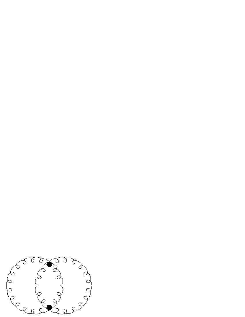
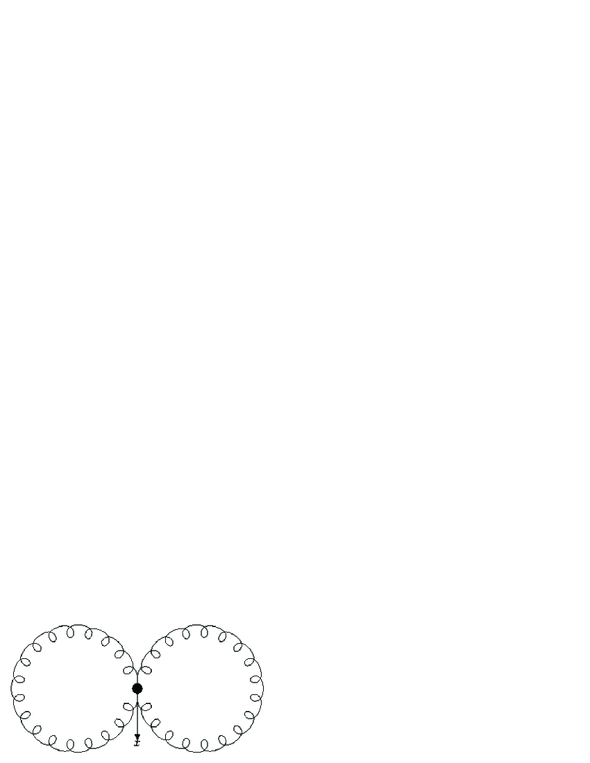
Figure 1: A $2PPI$ vacuum bubble.

Figure 2: A $2PPR$ vacuum bubble. $x$ is the $2PPR$ insertion point.

We may now resum this series of $2PPR$ and $2PPI$ graphs, where the propagators are the usual massless ones, by retaining only the $2PPI$ graphs, whereby the $2PPR$ insertions, or bubbles, are resummed into an effective $(\textrm{mass})^{2}$ $m_{2PPI}^{2}\equiv\overline{m}^{2}$. The bubble graph gluon polarization is then given by

$$\Pi^{ab}_{\mu\nu} = -~{}\frac{g^{2}}{2}\left[f_{eab}f_{ecd}\left(\left\langle A_{\mu}^{c}A_{\nu}^{d}\right\rangle-\left\langle A_{\mu}^{d}A_{\nu}^{c}\right\rangle\right)+f_{eac}f_{edb}\left(\left\langle A_{\mu}^{d}A_{\nu}^{c}\right\rangle-\left\langle A_{\rho}^{c}A_{\rho}^{d}\right\rangle\delta_{\mu\nu}\right)\right.$$ (2.2)

$$+~{}\left.f_{ead}f_{ebc}\left(\delta_{\mu\nu}\left\langle A_{\rho}^{c}A_{\rho}^{d}\right\rangle-\left\langle A_{\mu}^{c}A_{\nu}^{d}\right\rangle\right)\right]$$

where $f_{abc}$ are the $SU(N)$ structure constants. We define the vacuum expectation value of $A_{\mu}^{2}$ as

$$\Delta~{}=~{}\left\langle A_{\mu}^{a}A_{\mu}^{a}\right\rangle~{}.$$ (2.3)

The global $SU(N)$ symmetry can then be used to show that

$$\left\langle A_{\mu}^{a}A_{\nu}^{b}\right\rangle~{}=~{}\frac{\delta^{ab}\delta_{\mu\nu}}{d\left(N^{2}-1\right)}\Delta$$ (2.4)

Substitution of (2.4) in (2.2) yields

$$\Pi^{ab}_{\mu\nu}~{}=~{}-~{}g^{2}\frac{N}{N^{2}-1}\frac{d-1}{d}\delta^{ab}\delta_{\mu\nu}\Delta$$ (2.5)

which results in an effective mass, $\overline{m}$, running in the $2PPI$ propagators, given by

$$\overline{m}^{2}~{}=~{}g^{2}\frac{N}{N^{2}-1}\frac{d-1}{d}\Delta~{}.$$ (2.6)

If we let $E_{2PPI}$ be the sum of the $2PPI$ vacuum bubbles, calculated with the effective $2PPI$ propagator, then this $E_{2PPI}$ is not equal to the vacuum energy $E$, because simply removing all $2PPR$ insertions is too naive. For instance, there is a double counting problem which is already visible in the $2PPR$ diagram of Fig. 2 where each bubble can be seen as a $2PPR$ insertion on the other one. However, we can resolve this ambiguity. A dimensional argument results in

$$E~{}=~{}E_{2PPI}~{}+~{}cg^{2}\Delta^{2}$$ (2.7)

where $c\neq 0$ will accomodate the double counting. To determine the appropriate value of $c$, we use the path integral which gives

$$\frac{\partial E}{\partial g^{2}} = -~{}\frac{1}{4g}f_{abc}\left\langle\left(\partial_{\mu}A_{\nu}^{a}-\partial_{\nu}A_{\mu}^{a}\right)A_{\mu}^{b}A_{\nu}^{c}\right\rangle~{}-~{}\frac{1}{2g}f_{abc}\left\langle\partial_{\mu}\overline{\xi}^{a}\xi^{c}A_{\mu}^{b}\right\rangle$$ (2.8)

$$+~{}\frac{1}{4}f_{abc}f_{ade}\left\langle A_{\mu}^{b}A_{\nu}^{c}A_{\mu}^{d}A_{\nu}^{e}\right\rangle~{}.$$

The first two terms contribute unambiguously to the $2PPI$ part. For the last term, we rewrite

$$\left\langle A_{\mu}^{b}A_{\nu}^{c}A_{\mu}^{d}A_{\nu}^{e}\right\rangle = \left\langle A_{\mu}^{b}A_{\nu}^{c}\right\rangle\left\langle A_{\mu}^{d}A_{\nu}^{e}\right\rangle~{}+~{}\left\langle A_{\mu}^{b}A_{\mu}^{d}\right\rangle\left\langle A_{\nu}^{c}A_{\nu}^{e}\right\rangle$$ (2.9)

$$+~{}\left\langle A_{\mu}^{b}A_{\nu}^{e}\right\rangle\left\langle A_{\nu}^{c}A_{\mu}^{d}\right\rangle+\left\langle A_{\mu}^{b}A_{\nu}^{c}A_{\mu}^{d}A_{\nu}^{e}\right\rangle_{2PPI}~{}.$$

Using (2.4) and the properties of the structure constants $f_{abc}$, we obtain

$$\frac{\partial E}{\partial g^{2}} = -~{}\frac{1}{4g}f_{abc}\left\langle\left(\partial_{\mu}A_{\nu}^{a}-\partial_{\nu}A_{\mu}^{a}\right)A_{\mu}^{b}A_{\nu}^{c}\right\rangle_{2PPI}~{}-~{}\frac{1}{2g}f_{abc}\left\langle\partial_{\mu}\overline{\xi}^{a}\xi^{c}A_{\mu}^{b}\right\rangle_{2PPI}$$ (2.10)

$$+~{}\frac{1}{4}f_{abc}f_{ade}\left\langle A_{\mu}^{b}A_{\nu}^{c}A_{\mu}^{d}A_{\nu}^{e}\right\rangle_{2PPI}~{}+~{}\frac{1}{4}\frac{N}{N^{2}-1}\frac{d-1}{d}\Delta^{2}$$

$$= \frac{\partial E_{2PPI}}{\partial g^{2}}~{}+~{}\frac{1}{4}\frac{N}{N^{2}-1}\frac{d-1}{d}\Delta^{2}~{}.$$

From (2.7), we derive

$$\frac{\partial E}{\partial g^{2}}~{}=~{}\frac{\partial E_{2PPI}}{\partial g^{2}}~{}+~{}\frac{\partial E_{2PPI}}{\partial\overline{m}^{2}}\frac{\partial\overline{m}^{2}}{\partial g^{2}}~{}+~{}c\Delta^{2}+2cg^{2}\Delta\frac{\partial\Delta}{\partial g^{2}}~{}.$$ (2.11)

Combining (2.6), (2.10) and (2.11) gives

$$\frac{\partial E_{2PPI}}{\partial\overline{m}^{2}}\left(\frac{N}{N^{2}-1}\frac{d-1}{d}\Delta+g^{2}\frac{N}{N^{2}-1}\frac{d-1}{d}\frac{\partial\Delta}{\partial g^{2}}\right)~{}=~{}\frac{1}{4}\frac{N}{N^{2}-1}\frac{d-1}{d}\Delta^{2}~{}.$$ (2.12)

Then a simple diagrammatical argument gives

$$\frac{\partial E_{2PPI}}{\partial\overline{m}^{2}}~{}=~{}\frac{\Delta}{2}~{}.$$ (2.13)

which is a local gap equation, summing the bubble graphs into $\overline{m}^{2}$. Using this together with (2.12) finally gives

$$c~{}=~{}-~{}\frac{1}{4}\frac{N}{N^{2}-1}\frac{d-1}{d}~{}.$$ (2.14)

It is easy to show that the following equivalence holds

$$\frac{\partial E_{2PPI}}{\partial\overline{m}^{2}}~{}=~{}\frac{\Delta}{2}~{}\Leftrightarrow~{}\frac{\partial E}{\partial\overline{m}^{2}}~{}=~{}0~{}.$$ (2.15)

To summarize, we have summed the bubble insertions into an effective $(\textrm{mass})^{2}$, $\overline{m}^{2}$. The vacuum energy is expressed by

$$E~{}=~{}E_{2PPI}~{}-~{}\frac{g^{2}}{4}\frac{N}{N^{2}-1}\frac{d-1}{d}\Delta^{2}~{}.$$ (2.16)

We stress the fact that (2.16) is only meaningful if the gap equation (2.15) is satisfied. This means we cannot consider $\overline{m}$ or $\Delta$ as a real variable on which $E$ depends. It is a quantity which has to obey its gap equation, otherwise the $2PPI$ expansion loses its validity. This also means that $E(\overline{m})$, or equivalently $E(\Delta)$, is not a function depending on $\overline{m}$ ($\Delta$), in contrast with the usual concept of an effective potential $V(\varphi)$ which is a function of the constant field $\varphi$.

In order to ensure the usefulness of the $2PPI$ formalism for actual calculations, we should prove it can be fully renormalized with the counterterms available from the original (bare) Lagrangian, (2.1). However, it is sufficient to say that all our derived formulae remain valid and are finite when the counterterms are included. This also implies the $2PPI$ mass $\overline{m}$ is renormalized and gives rise to a finite, physical mass, $m_{\mbox{\footnotesize{{phys}}}}$. Furthermore, no new counterterms are needed to remove the vacuum energy divergences. The renormalizability of the $2PPI$ expansion has been discussed in detail in [27] in the case of the Gross-Neveu model. Since the arguments for Yang Mills theory are completely analogous, we refer to [27] for technical details concerning the renormalization.

Another point worth emphasising here, is the renormalization group equation, (RGE), for $E$. The first diagram of $E_{2PPI}$ is given by the O-bubble. Using the $\overline{\mbox{MS}}$ renormalization scheme in dimensional regularization in $d$ dimensions, we find

$$E~{}=~{}\frac{3}{4}\frac{N^{2}-1}{16\pi^{2}}\overline{m}^{4}\left(\ln\frac{\overline{m}^{2}}{\overline{\mu}^{2}}-\frac{5}{6}\right)~{}-~{}\frac{1}{4\overline{g}^{2}}\frac{d}{d-1}\frac{N^{2}-1}{N}\overline{m}^{4}~{}.$$ (2.17)

Since $E$ is a physical quantity, it should not depend on the subtraction scale $\overline{\mu}$. This is expressed by the RGE

$$\overline{\mu}\frac{dE}{d\overline{\mu}}~{}=~{}\left(\overline{\mu}\frac{\partial}{\partial\overline{\mu}}~{}+~{}\overline{\beta}(\overline{g}^{2})\frac{\partial}{\partial\overline{g}^{2}}~{}+~{}\overline{\kappa}(\overline{g}^{2})\overline{m}^{2}\frac{\partial}{\partial\overline{m}^{2}}\right)E~{}=~{}0$$ (2.18)

where $\overline{\beta}(\overline{g}^{2})$ governs the scaling behaviour of the coupling constant

$$\overline{\beta}(\overline{g}^{2})~{}=~{}\overline{\mu}\frac{\partial\overline{g}^{2}}{\partial\overline{\mu}}~{}=~{}-~{}2\left(\beta_{0}\overline{g}^{4}~{}+~{}\beta_{1}\overline{g}^{6}~{}+~{}\overline{\beta}_{2}\overline{g}^{8}~{}+~{}\cdots\right)$$ (2.19)

and $\overline{\kappa}(\overline{g}^{2})$ is the anomalous dimension of $\overline{m}^{2}$

$$\overline{\mu}\frac{\partial\overline{m}^{2}}{\partial\overline{\mu}} = \left(\frac{\overline{\beta}(\overline{g}^{2})}{\overline{g}^{2}}~{}+~{}\overline{\gamma}_{A_{\mu}^{2}}(\overline{g}^{2})\right)\overline{m}^{2}~{}\equiv~{}\overline{\kappa}(\overline{g}^{2})\overline{m}^{2}$$ (2.20)

$$\overline{\gamma}_{A_{\mu}^{2}}(\overline{g}^{2}) = \frac{\overline{\mu}}{\overline{\Delta}}\frac{\partial\overline{\Delta}}{\partial\overline{\mu}}~{}=~{}\gamma_{0}\overline{g}^{2}~{}+~{}\overline{\gamma}_{1}\overline{g}^{4}~{}+~{}\overline{\gamma}_{2}\overline{g}^{6}~{}+~{}\cdots~{}.$$ (2.21)

The coefficients can be found in [28, 29] for $\overline{\beta}$ and in [26, 29, 30] for $\overline{\gamma}_{A_{\mu}^{2}}$,

$$\beta_{0} = \frac{11}{3}\left(\frac{N}{16\pi^{2}}\right)\hskip 28.45274pt\beta_{1}~{}=~{}\frac{34}{3}\left(\frac{N}{16\pi^{2}}\right)^{2}\hskip 28.45274pt\overline{\beta}_{2}~{}=~{}\frac{2857}{54}\left(\frac{N}{16\pi^{2}}\right)^{3}$$ (2.22)

$$\gamma_{0} = \frac{35}{6}\left(\frac{N}{16\pi^{2}}\right)\hskip 28.45274pt\overline{\gamma}_{1}~{}=~{}\frac{449}{24}\left(\frac{N}{16\pi^{2}}\right)^{2}\hskip 28.45274pt\overline{\gamma}_{2}~{}=~{}\left[\frac{75607}{864}-\frac{9\zeta(3)}{16}\right]\left(\frac{N}{16\pi^{2}}\right)^{3}~{}.$$

When we combine all this information and determine $\overline{\mu}\frac{dE}{d\overline{\mu}}$ up to lowest order in $\overline{g}^{2}$, we find

$$\overline{\mu}\frac{dE}{d\overline{\mu}}~{}\neq~{}0~{}.$$ (2.24)

Apparently, it seems that $E$ does not obey its RGE. However, this is not a contradiction because of the demand that the gap equation (2.15) must be satisfied. The gap equation implies that $\ln\frac{\overline{m}^{2}}{\overline{\mu}^{2}}\propto\frac{1}{\overline{g}^{2}}+\textrm{constants}$. The consequence is that all leading logarithms contain terms of order unity. Hence, we cannot show that the RGE for $E$ is obeyed order by order. The same phenomenon extends to higher orders. In other words, knowledge of $\overline{\mu}\frac{dE}{d\overline{\mu}}$ up to a certain order $n$, would require knowledge of all leading and subleading log terms to order $n$, to show explicitly that $\overline{\mu}\frac{dE}{d\overline{\mu}}$ $=$ $0$. We must therefore be careful not to interpret the non-vanishing of the RGE as a reason to introduce a “non-perturbative” $\beta$-function, as is sometimes done, [31].

3 Results.

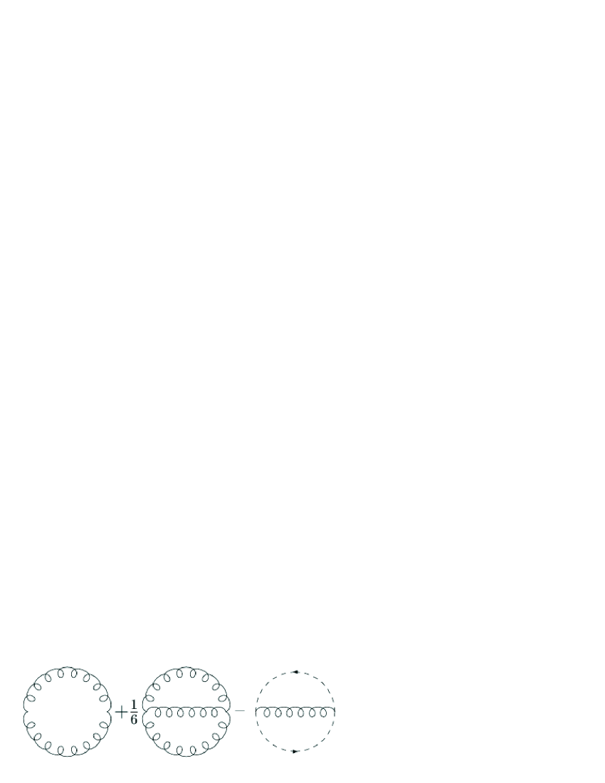
Figure 3: The first diagrams contributing to $E_{2PPI}$

Up to 2-loop order in the $2PPI$ expansion (see Fig. 3), we find in the $\overline{\mbox{MS}}$ scheme

$$E(\overline{\Delta}) = -~{}\frac{3}{16}\frac{\overline{g}^{2}N}{N^{2}-1}\overline{\Delta}^{2}~{}+~{}\frac{27}{64}\frac{\overline{g}^{4}N^{2}}{16\pi^{2}}\frac{\overline{\Delta}^{2}}{N^{2}-1}\left(\ln\frac{\frac{3}{4}\frac{\overline{g}^{2}N}{N^{2}-1}\overline{\Delta}}{\overline{\mu}^{2}}-\frac{5}{6}\right)~{}+~{}\frac{9}{16}\frac{\overline{g}^{6}N^{3}}{\left(16\pi^{2}\right)^{2}}\frac{\overline{\Delta}^{2}}{N^{2}-1}$$

$$\times~{}\left[-\frac{31}{2}\left(\ln\frac{\frac{3}{4}\frac{\overline{g}^{2}N}{N^{2}-1}\overline{\Delta}}{\overline{\mu}^{2}}\right)^{2}~{}+~{}\frac{259}{8}\ln\frac{\frac{3}{4}\frac{\overline{g}^{2}N}{N^{2}-1}\overline{\Delta}}{\overline{\mu}^{2}}~{}-~{}\frac{1043}{32}~{}+~{}\frac{891}{16}s_{2}~{}-~{}\frac{63}{8}\zeta(2)\right]$$

where $\zeta(n)$ is the Riemann zeta function,

$$s_{2}~{}=~{}\frac{4}{9\sqrt{3}}\mathcal{C}\ell_{2}\left({\frac{\pi}{3}}\right)~{}\approx~{}0.2604341$$ (3.2)

and $\mathcal{C}\ell_{2}(x)$ is the Clausen function. We have computed the relevant two loop vacuum bubble diagrams to the finite part using the massive gluon and massless ghost propagators which are respectively

$$-~{}\frac{1}{p^{2}+\overline{m}^{2}}\left[\delta_{\mu\nu}~{}-~{}\frac{p_{\mu}p_{\nu}}{p^{2}}\right]~{}~{}~{}~{}~{}\mbox{and}~{}~{}~{}~{}~{}\frac{1}{p^{2}}$$ (3.3)

in the Landau gauge. The expressions for the general massive and massless two loop bubble integrals were derived from the results of [32] and implemented in the symbolic manipulation language Form, [33]. It is easy to check that solving the gap equation $\frac{\partial E}{\partial\overline{\Delta}}$ $=$ $0$, with $\overline{\mu}^{2}$ set equal to $\frac{3}{4}\frac{\overline{g}^{2}N}{N^{2}-1}\overline{\Delta}$ to kill potentially large logarithms, gives no solution at 1-loop or 2-loop, apart from the trivial one $\overline{\Delta}$ $=$ $0$. This does not imply $\left\langle A_{\mu}^{2}\right\rangle$ does not exist but that the $\overline{\mbox{MS}}$ scheme might not be the best choice for the $2PPI$ expansion. To address this we first remove the freedom existing in how the mass parameter $\Delta$ is renormalized by replacing $\Delta$ by a renormalization scheme and scale independent quantity $\widetilde{\Delta}$. This can be accommodated by

$$\widetilde{\Delta}~{}=~{}\overline{f}\left(\overline{g}^{2}\right)\overline{\Delta}$$ (3.4)

with

$$\overline{\mu}\frac{\partial\overline{f}}{\partial\overline{\mu}}~{}=~{}-~{}\overline{\gamma}_{A_{\mu}^{2}}\left(\overline{g}^{2}\right)\overline{f}~{}.$$ (3.5)

A change in massless renormalization scheme corresponds to relations of the form

$$\overline{g}^{2} = g^{2}\left(1+b_{0}g^{2}+b_{1}g^{4}+\cdots\right)$$ (3.6)

$$\overline{\Delta} = \Delta\left(1+d_{0}g^{2}+d_{1}g^{4}+\cdots\right)$$ (3.7)

$$\overline{f}(\overline{g}^{2}) = f(g^{2})\left(1+f_{0}g^{2}+f_{1}g^{4}+\cdots\right)~{}.$$ (3.8)

With these, it is easily checked that (3.4) is renormalization scheme and scale independent. The explicit solution of (3.5) reads

$$\overline{f}\left(\overline{g}^{2}\right) = \left(\overline{g}^{2}\right)^{\frac{\gamma_{0}}{2\beta_{0}}}\left\{1\vphantom{\frac{\gamma_{0}\left(\frac{\beta_{1}^{2}}{\beta_{0}^{2}}-\frac{\overline{\beta}_{2}}{\beta_{0}}\right)}{\beta_{0}}}+\frac{\overline{g}^{2}}{2}\left(-\frac{\beta_{1}\gamma_{0}}{\beta_{0}^{2}}+\frac{\overline{\gamma}_{1}}{\beta_{0}}\right)+\frac{\overline{g}^{4}}{4}\left[\vphantom{\frac{\gamma_{0}\left(\frac{\beta_{1}^{2}}{\beta_{0}^{2}}-\frac{\overline{\beta}_{2}}{\beta_{0}}\right)}{\beta_{0}}}\frac{1}{2}\left(-\frac{\beta_{1}\gamma_{0}}{\beta_{0}^{2}}+\frac{\overline{\gamma}_{1}}{\beta_{0}}\right)^{2}\right.\right.$$ (3.9)

$$+~{}\left.\left.\frac{\gamma_{0}\left(\frac{\beta_{1}^{2}}{\beta_{0}^{2}}-\frac{\overline{\beta}_{2}}{\beta_{0}}\right)}{\beta_{0}}-\frac{\beta_{1}\overline{\gamma}_{1}}{\beta_{0}^{2}}+\frac{\overline{\gamma}_{2}}{\beta_{0}}\right]+\mathcal{O}\left(\overline{g}^{6}\right)\right\}~{}.$$

Since the gap equation is still a series expansion in $\frac{g^{2}N}{16\pi^{2}}$ and we hope to find (at least qualitatively) acceptable results, $\frac{g^{2}N}{16\pi^{2}}$ should be small. We will therefore choose to renormalize the coupling constant in such a scheme so that $E$ is of the form

$$E~{}=~{}\frac{3}{16}\left(g^{2}\right)^{1-\frac{\gamma_{0}}{\beta_{0}}}\frac{N}{N^{2}-1}\widetilde{\Delta}^{2}\left(-1+\frac{g^{2}N}{16\pi^{2}}E_{1}^{1}L+\left(\frac{g^{2}N}{16\pi^{2}}\right)^{2}\left(E_{2}^{1}L+E_{2}^{2}L^{2}\right)+\ldots\right)$$ (3.10)

where

$$L~{}=~{}\ln\frac{\frac{3}{4}\left(g^{2}\right)^{1-\frac{\gamma_{0}}{2\beta_{0}}}\frac{N}{N^{2}-1}\widetilde{\Delta}}{\overline{\mu}^{2}}~{}.$$ (3.11)

Otherwise, we remove all the terms of the form $\left(\frac{g^{2}N}{16\pi^{2}}\right)^{n}\times\textrm{constant}$, and only keep the terms that contain a power of the logarithm $L$. This is always possible by calculating the $\overline{\mbox{MS}}$ value of $E$ as in (3) and using (3.6) to change the coupling constant renormalization by a suitable choice for the coefficients $b_{i}$. In other words the 1-loop $\overline{\mbox{MS}}$ contribution to $E$ allows one to determine $b_{0}$. Once $b_{0}$ is fixed, the 2-loop $\overline{\mbox{MS}}$ contribution to $E$ can be used to fix $b_{1}$, and so on for the higher order contributions. We note that the gap equation (2.15) is translated into $\frac{\partial E}{\partial\widetilde{\Delta}}$ $=$ $0$ since $\overline{m}^{2}\propto\overline{\Delta}\propto\widetilde{\Delta}$. In this gap equation, we will set $\overline{\mu}^{2}$ $=$ $\frac{3}{4}\left(g^{2}\right)^{1-\frac{\gamma_{0}}{2\beta_{0}}}\frac{N}{N^{2}-1}\widetilde{\Delta}$ so that all logarithms vanish. In other words $L$ $=$ $0$. Notice that one cannot set $\overline{\mu}^{2}$ $=$ $\frac{3}{4}\left(g^{2}\right)^{1-\frac{\gamma_{0}}{2\beta_{0}}}\frac{N}{N^{2}-1}\widetilde{\Delta}$ in the expression (3.10) and use the RGE for $E$ to sum the logarithms when $\frac{dE}{d\widetilde{\Delta}}=0$ is solved. As already explained in the previous section, the RGE for $E$ is not obeyed order by order, see also [27]. Once a solution $\widetilde{\Delta}_{*}$ of the gap equation is found, then we will always have

$$E_{\mbox{\footnotesize{{vac}}}}~{}=~{}-~{}\frac{3}{16}\left(g^{2}\right)^{1-\frac{\gamma_{0}}{\beta_{0}}}\frac{N}{N^{2}-1}\widetilde{\Delta}_{*}^{2}~{}.$$ (3.12)

If the constructed value for $\frac{g^{2}N}{16\pi^{2}}$ is small enough, then we can trust, at least qualitatively, the results we will obtain. Now we are ready to rewrite (3) in terms of $\widetilde{\Delta}$. After a little algebra, one finds

$$E = \frac{3}{16}\left(g^{2}\right)^{1-\frac{\gamma_{0}}{\beta_{0}}}\frac{N}{N^{2}-1}\widetilde{\Delta}^{2}\left\{-1+\left[\frac{9N}{64\pi^{2}}\left(-\frac{5}{6}+L\right)-2c_{1}-c_{4}\right]g^{2}\right.$$

$$+~{}\left.\left[\frac{3N^{2}}{256\pi^{4}}\left(c_{3}+\frac{259}{8}L-\frac{31}{2}L^{2}\right)-2b_{0}c_{1}-c_{1}^{2}-2c_{2}+\left(\frac{9N}{64\pi^{2}}\left(-\frac{5}{6}+L\right)-2c_{1}\right)c_{4}\right.\right.$$

$$-~{}c_{5}+\left.\left.\frac{9N}{64\pi^{2}}\left(\left(-\frac{5}{6}+L\right)b_{0}+c_{1}+2\left(-\frac{5}{6}+L\right)c_{1}+b_{0}\left(1-\frac{\gamma_{0}}{2\beta_{0}}\right)\right)\right]g^{4}+\mathcal{O}\left(g^{6}\right)\right\}$$

with

$$c_{1} = \frac{1}{2}\left(\frac{\beta_{1}\gamma_{0}}{\beta_{0}^{2}}-\frac{\overline{\gamma}_{1}}{\beta_{0}}\right)$$ (3.14)

$$c_{2} = \frac{1}{8}\left(-\frac{\beta_{1}\gamma_{0}}{\beta_{0}^{2}}+\frac{\overline{\gamma}_{1}}{\beta_{0}}\right)^{2}-\frac{1}{4}\left(\frac{\gamma_{0}\left(\frac{\beta_{1}^{2}}{\beta_{0}^{2}}-\frac{\overline{\beta}_{2}}{\beta_{0}}\right)}{\beta_{0}}\right)+\frac{1}{4}\left(\frac{\beta_{1}\overline{\gamma}_{1}}{\beta_{0}^{2}}-\frac{\overline{\gamma}_{2}}{\beta_{0}}\right)$$ (3.15)

$$c_{3} = -~{}\frac{1043}{32}-\frac{63}{8}\zeta(2)+\frac{891}{16}s_{2}$$ (3.16)

$$c_{4} = b_{0}\left(1-\frac{\gamma_{0}}{\beta_{0}}\right)$$ (3.17)

$$c_{5} = b_{1}\left(1-\frac{\gamma_{0}}{\beta_{0}}\right)-b_{0}^{2}\frac{\gamma_{0}}{2\beta_{0}}\left(1-\frac{\gamma_{0}}{\beta_{0}}\right)~{}.$$ (3.18)

Next, we determine $b_{0}$ and $b_{1}$ so that (3) reduces to

$$E = \frac{3}{16}\left(g^{2}\right)^{1-\frac{\gamma_{0}}{\beta_{0}}}\widetilde{\Delta}^{2}\frac{N}{N^{2}-1}\left\{-1+g^{2}\frac{9N}{64\pi^{2}}L+g^{4}\left[\frac{3N^{2}}{256\pi^{4}}\left(\frac{259}{8}L-\frac{31}{2}L^{2}\right)\right.\right.$$ (3.19)

$$+~{}\left.\left.\frac{9N}{64\pi^{2}}\left(b_{0}+c_{4}+2c_{1}\right)L\right]+\mathcal{O}\left(g^{6}\right)\right\}~{}.$$

We find that $b_{0}$ is

$$b_{0}~{}=~{}\frac{409}{2288}\frac{N}{\pi^{2}}~{}.$$ (3.20)

We do not list the value for $b_{1}$ since it is no longer required. From the $\beta$-function we find the two loop expression for the coupling constant is

$${g}^{2}(\overline{\mu}) = \frac{1}{\beta_{0}\ln\frac{\overline{\mu}^{2}}{\Lambda^{2}}}-\frac{\beta_{1}}{\beta_{0}}\frac{\ln\ln\frac{\overline{\mu}^{2}}{\Lambda^{2}}}{\beta_{0}^{2}\ln^{2}\frac{\overline{\mu}^{2}}{\Lambda^{2}}}$$ (3.21)

where $\Lambda$ is the scale parameter of the corresponding massless renormalization scheme. We will express everything in terms of the $\overline{\mbox{MS}}$ scale parameter $\Lambda_{\overline{\mbox{\footnotesize{MS}}}}$. In [34], it was shown that

$$\Lambda~{}=~{}\Lambda_{\overline{\mbox{\footnotesize{MS}}}}e^{-\frac{b_{0}}{2\beta_{0}}}~{}.$$ (3.22)

We will also derive a value for the $\left\langle\frac{\alpha_{s}}{\pi}G_{\mu\nu}^{2}\right\rangle$ condensate from the trace anomaly

$$\Theta_{\mu\mu}~{}=~{}\frac{\beta(g)}{2g}\left(G^{a}_{\rho\sigma}\right)^{2}~{}.$$ (3.23)

This anomaly allows us to deduce for $N$ $=$ $3$ the following relation between the vacuum energy and the gluon condensate

$$\left\langle\frac{\alpha_{s}}{\pi}G_{\mu\nu}^{2}\right\rangle~{}=~{}-~{}\frac{32}{11}E_{\mbox{\footnotesize{{vac}}}}~{}.$$ (3.24)

At 1-loop order, the results for $N$ $=$ $3$ are

$$\left.\frac{g^{2}N}{16\pi^{2}}\right|_{\mbox{\footnotesize{{1-loop}}}} = \frac{8}{9}$$ (3.25)

$$\left.\sqrt{\widetilde{\Delta}}\right|_{\mbox{\footnotesize{{1-loop}}}} \approx 1.004\Lambda_{\overline{\mbox{\footnotesize{MS}}}}\approx 233\textrm{MeV}$$ (3.26)

$$\left.E_{\mbox{\footnotesize{{vac}}}}\right|_{\mbox{\footnotesize{{1-loop}}}} \approx -0.0074\Lambda_{\overline{\mbox{\footnotesize{MS}}}}^{4}~{}\approx~{}-~{}0.00002\textrm{GeV}^{4}$$ (3.27)

$$\left.\left\langle\frac{\alpha_{s}}{\pi}G_{\mu\nu}^{2}\right\rangle\right|_{\mbox{\footnotesize{{1-loop}}}} \approx 0.02\Lambda_{\overline{\mbox{\footnotesize{MS}}}}^{4}~{}\approx~{}0.00007\textrm{GeV}^{4}$$ (3.28)

while the scale parameter $\overline{\mu}^{2}\approx(184\textrm{MeV})^{2}$. We have used $\Lambda_{\overline{\mbox{\footnotesize{MS}}}}$ $\approx$ $233\textrm{MeV}$ which was the value reported in [11]. We see that the 1-loop expansion parameter is quite large and we conclude that we should go to the next order where the situation is improved. We find

$$\left.\frac{g^{2}N}{16\pi^{2}}\right|_{\mbox{\footnotesize{{2-loop}}}} \approx 0.131$$ (3.29)

$$\left.\sqrt{\widetilde{\Delta}}\right|_{\mbox{\footnotesize{{2-loop}}}} \approx 2.3\Lambda_{\overline{\mbox{\footnotesize{MS}}}}~{}\approx~{}536\textrm{MeV}$$ (3.30)

$$\left.E_{\mbox{\footnotesize{{vac}}}}\right|_{\mbox{\footnotesize{{2-loop}}}} \approx -0.63\Lambda_{\overline{\mbox{\footnotesize{MS}}}}^{4}~{}\approx~{}-~{}0.002\textrm{GeV}^{4}$$ (3.31)

$$\left.\left\langle\frac{\alpha_{s}}{\pi}G_{\mu\nu}^{2}\right\rangle\right|_{\mbox{\footnotesize{{2-loop}}}} \approx 1.84\Lambda_{\overline{\mbox{\footnotesize{MS}}}}^{4}~{}\approx~{}0.005\textrm{GeV}^{4}~{}.$$ (3.32)

with $\overline{\mu}^{2}\approx(347\textrm{MeV})^{2}$. Although there is a sizeable difference between 1-loop and 2-loop results, the relative smallness of the 2-loop expansion parameter, indicates that the 2-loop values are qualitatively trustworthy. It is well known that in order to find reliable perturbative results, one must go beyond 1-loop, and even beyond 2-loop approximations. Therefore, one should not attach a firm quantitative meaning to the numerical values. Let us compare our results with what was found elsewhere with different methods. A combined lattice fit resulted in $\sqrt{\left\langle A_{\mu}^{2}\right\rangle}$ $\approx$ $1.64\textrm{GeV}$, [11]. We cannot really compare this with our result for $\sqrt{\widetilde{\Delta}}$, since the lattice value was obtained with the OPE at a scale $\mu$ $=$ $10\textrm{GeV}$ in a specific renormalization scheme (MOM). However, it is satisfactory that (3.30) is at least of the same order of magnitude. More interesting is the comparison with what was found in [26] with the local composite operator formalism for $\left\langle A_{\mu}^{2}\right\rangle$. In the $\overline{\mbox{MS}}$ scheme at 2-loop order, it was found that $\frac{\overline{g}^{2}N}{16\pi^{2}}\approx 0.141247$ while $E_{\mbox{\footnotesize{{vac}}}}$ $\approx$ $-\,0.789\Lambda_{\overline{\mbox{\footnotesize{MS}}}}^{4}$ which is in quite good agreement with our results. An estimate of the tree level gluon mass of $\sim 500\textrm{MeV}$ was also given in [26] which compares well with the lattice value of $\sim 600\textrm{MeV}$ of [35, 36]. With the $2PPI$ method, one does not really have the concept of a tree level mass. Instead, the determination of $m_{\mbox{\footnotesize{{phys}}}}$ would need the calculation of the highly non-trivial 2-loop $2PPI$ mass renormalization graphs which is beyond the scope of this article.

In conclusion we note that the perturbative Yang-Mills vacuum is unstable and lowers its value through a non-perturbative mass dimension two gluon condensate $\left\langle A_{\mu}^{2}\right\rangle$. We have omitted quark contributions in our analysis but it is straighforward to extend the $2PPI$ expansion to QCD with quarks included. Indeed an idea of the effect they have could be gained by an extension of [26].

Acknowledgement. This work was supported in part by Pparc through a research studentship, (REB).

- [1] K.G. Chetyrkin, S. Narison & V.I. Zakharov, Nucl. Phys. B 550 (1999), 353.
- [2] F.V. Gubarev, L. Stodolsky & V.I. Zakharov, Phys. Rev. Lett. 86 (2001), 2220.
- [3] F.V. Gubarev & V.I. Zakharov, Phys. Lett. B 501 (2001), 28.
- [4] D.J. Gross & A. Neveu, Phys. Rev. D 10 (1974), 3235.
- [5] H. Verschelde, Phys. Lett. B 497 (2001), 165.
- [6] G. Smet, T. Vanzieleghem, K. Van Acoleyen & H. Verschelde, Phys. Rev. D 65 (2002), 045015.
- [7] R. Fukuda & T. Kugo, Prog. Theor. Phys. 60 (1978), 565.
- [8] R. Fukuda, Phys. Lett. B 73 (1978) 33; erratum ibid. B 74 (1978), 433.
- [9] V. P. Gusynin & V. A. Miransky, Phys. Lett. B 76 (1978) 585.
- [10] G. K. Savvidy, Phys. Lett. B 71 (1977) 133.
- [11] P. Boucaud, A. Le Yaouanc, J.P. Leroy, J. Micheli, O. Pne & J. Rodriguez-Quintero, Phys. Rev. D 63 (2001), 114003.
- [12] P. Boucaud, J.P. Leroy, A. Le Yaounac, J. Micheli, O. Pène, F. De Soto, A. Donini, H. Moutarde & J. Rodriguez-Quintero, Phys. Rev. D 66 (2002), 034504.
- [13] L. Stodolsky, P. van Baal & V.I. Zakharov, Phys. Lett. B 552 (2003), 214.
- [14] G. Curci & R. Ferrari, Nuovo Cim. A 32 (1976), 151.
- [15] G. Curci & R. Ferrari, Phys. Lett. B 63 (1976), 91.
- [16] K.I. Kondo, Phys. Lett. B 514 (2001), 335.
- [17] K.I. Kondo, T. Murakami, T. Shinohara & T. Imai, Phys. Rev. D 65 (2002), 085034.
- [18] K. Langfeld, in ‘Confinement, Topology and other Non-perturbative Aspects of QCD’ edited by Jeff Greensite & tefan Olejnk, NATO Science Series, 253-260, hep-lat/0204025.
- [19] P.O. Bowman, U.M. Heller, D.B. Leinweber & A.G. Williams, Phys. Rev. D 66 (2002), 074505.
- [20] F.D. Bonnet, P.O. Bowman, D.B. Leinweber, A.G. Williams & J.M. Zanotti, Phys. Rev. D 64 (2001), 034501.
- [21] C. Alexandrou, P. de Forcrand & E. Follana, Phys. Rev. D 63 (2001), 094504.
- [22] R. Alkofer & L. von Smekal, Nucl. Phys. A 680 (2000), 133.
- [23] R. Alkofer & L. von Smekal, Phys. Rept. 353 (2001), 281.
- [24] C. Lerche & L. von Smekal, Phys. Rev. D 65 (2002), 125006.
- [25] K.I. Kondo & T. Imai, hep-th/0206173.
- [26] H. Verschelde, K. Knecht, K. Van Acoleyen & M. Vanderkelen, Phys. Lett. B 516 (2001), 307, Erratum-ibid. Phys. Lett. B to appear.
- [27] D. Dudal & H. Verschelde, Phys. Rev. D67 (2003), 025011.
- [28] D.J. Gross & F.J. Wilczek, Phys. Rev. Lett. 30 (1973), 1343; H.D. Politzer, Phys. Rev. Lett. 30 (1973), 1346; D.R.T. Jones, Nucl. Phys. B75 (1974), 531; W.E. Caswell, Phys. Rev. Lett. 33 (1974), 244; O.V. Tarasov & A.A. Vladimirov, Sov. J. Nucl. Phys. 25 (1977), 585; E. Egorian & O.V. Tarasov, Theor. Math. Phys. 41 (1979), 863; S.A. Larin & J.A.M. Vermaseren, Phys. Lett. B303 (1993), 334.
- [29] J.A. Gracey, Phys. Lett. B 552 (2003), 101.
- [30] D. Dudal, H. Verschelde & S.P. Sorella, Phys. Lett. B 555 (2003), 126.
- [31] J.F. Yang & J.H. Ruan, Phys. Rev. D 65 (2002), 125009.
- [32] C. Ford, I. Jack & D.R.T. Jones, Nucl. Phys. B 387 (1992), 373.
- [33] J.A.M. Vermaseren, math-ph/0010025.
- [34] W. Celmaster & R.J. Gonsalves, Phys. Rev. D 20 (1979), 1420.
- [35] C. Alexandrou, P. de Forcrand & E. Follana, Phys. Rev. D 65 (2002), 114508.
- [36] K. Langfeld, H. Reinhardt & J. Gattnar, Nucl. Phys. B 621 (2002), 131.