December, 2002

Worldsheet Description of Tachyon
Condensation in Open String Theory
Tadaoki Uesugi

Department of Physics, Faculty of Science
University of Tokyo
Tokyo 113-0033, Japan
A Dissertation in candidacy for
the degree of Doctor of Philosophy

In this thesis we review the fundamental framework of boundary string field theory (BSFT) and apply it to the tachyon condensation on non-BPS systems in the superstring theory. The boundary string field theory can be regarded as a natural extension of the nonlinear sigma model. By using this theory we can describe the tachyon condensation exactly and also obtain the effective actions on non-BPS systems consisting of the Dirac-Born-Infeld type action and the Wess-Zumino type action. Especially the Wess-Zumino action is written by superconnection and coincides with the mathematical argument by K-theory. Moreover we also discuss the tachyon condensation keeping the conformal invariance (on-shell). The exact argument by using the boundary state formalism gives a good support to the conjecture of the tachyon condensation and it is also consistent with boundary string field theory.

Chapter 1 Introduction

In recent several years there has been tremendous progress in the nonperturbative aspect of string theory. One of key ingredients of this is the discovery of D-branes [1]. The D-branes are nonperturbative objects (solitons) in string theory which are considered to play the same role as instantons in gauge theory. Another important discovery is the string duality. The string duality unifies five supersymmetric string theories in a single framework called M-theory [2]. These two important discoveries have caused the recent development of string theory such as the matrix theory [3] and AdS/CFT [4] correspondence.

The important thing here is that the above progress has often relied on the existence of vast degrees of supersymmetry in the target space. So, the natural question is what we can find in the less or no supersymmetric structure of string theory. In the less supersymmetric phases of string theory we can expect that some dynamical phenomena happen in the same way as the confinement of quarks in less supersymmetric gauge theory. Since we do not understand the dynamical aspect of string theory very well, it is meaningful and theoretically interesting to study it.

On the other hand we already know that we can realize spontaneously broken phases of the supersymmetry in superstring theories by appropriate compactification or putting D-branes. In the latter point of view non-BPS D-brane systems can be regarded as one of simple models we can consider in order to investigate the structure of string theory without supersymmetry. Especially there are two kinds of D-brane systems without any supersymmetry in the flat space background of Type II theory. They are the brane-antibrane system and the non-BPS D-brane. Although of course several other kinds of non-BPS systems exist in string theory, D-branes are convenient objects we can deal with by using the conventional open string theory [1]. If we examine the open string spectrum on these non-BPS systems, we can see that tachyonic modes appear even though there are no tachyonic modes in the closed string spectrum. In the early stage of string theory as a dual model [5], the tachyonic modes were interpreted as the inconsistency of the theory. The recent idea about the interpretation of the tachyonic mode is that the theory is not inconsistent but stays in an unstable phase and will decay to a stable phase where full or some of the supersymmetries are restored.

Several years ago Ashoke Sen [6] conjectured that these unstable D-brane systems decay to the vacuum without any D-branes or other stable D-branes. This dynamical decay process is called tachyon condensation [6]. Since then there has been a lot of work about the verification of this conjecture in the quantitative way (for a review see [7]). However, it seems that in general we can not examine this by the conventional open string theory because this process relates two different backgrounds in string theory. One is an unstable background due to the existence of unstable D-branes and the other is a stable background where all or some supersymmetries are unbroken. What the conventional perturbative string theory can do is to examine the fluctuations and to calculate their scattering amplitudes around the fixed background, and it can not predict how two different backgrounds are related with each other. Therefore, we can say that this is an important problem of nonperturbative aspects of string theory in the same sense as the fact that the string duality has related various different string theories (vacuums) with each other. Indeed for several years a lot of methods have been developed and by using them Sen’s conjecture of the tachyon condensation has been checked. They include the noncommutaive field theory [8, 9, 10], K-theory [11, 12, 13, 14] and string field theory.

In this thesis we will investigate the tachyon condensation mainly by using open string field theory. This is a kind of “field theory” for open strings. If it has a feature similar to the field theory with a kind of scalar potential, we can relate two different backgrounds in string theory with each other as a maximum point and a minimum one of the scalar potential, which can not be done by the conventional perturbative string theory. Indeed, string field theory has that kind of potential called tachyon potential because there appears a scalar field which is a tachyon on unstable D-branes. In this sense this theory is well suited to verify Sen’s conjecture.

For now two types of covariant formulations of open string field theory are known. One is Witten’s cubic string field theory (CSFT) [15, 16] or Berkovits’ extended formulation for the superstring [17]. By using these formulations the conjecture of tachyon condensation has been checked [18, 19, 20]. Especially the approximate method called the level truncation has been used to calculate the tachyon potential. These analyses have shown that Sen’s conjecture is correct in the good accuracy (For a good review see [21] and references there in).

On the other hand there is the other type of string field theory. It is called boundary string field theory (BSFT), which is also constructed by Witten [22, 23, 24]. This formalism is quite different from the cubic string field theory. The most important fact is that this formalism enables us to calculate quantities like tachyon potential in the exact way [25, 26, 27, 28, 29], which might not be done by the cubic string field theory. In this sense this formalism has almost completed the verification of Sen’s conjecture, although there remain other related problems which we will mention in the final chapter.

The most characteristic feature in boundary string field theory is the fact that this theory can be regarded as a natural extension [30, 31, 32, 33, 34] of the two-dimensional nonlinear sigma model. Therefore we can apply the worldsheet picture in the conventional perturbative string theory even to the boundary string field theory, and in this sense the worldsheet description is a key word in the title of this thesis.

By the way, historically speaking, before the string field theory was used the other method [35, 36, 37, 38, 39, 40, 41, 42, 43, 44, 45, 46, 47] had been applied to prove some part of Sen’s conjecture (for a review see the papers [7, 48]). In the other paragraphs we have said that in general we can not use the conventional perturbative string theory for the tachyon condensation. However, in some special situations we can apply it and describe the tachyon condensation exactly. We will also explain this method in this thesis.

The organization of this thesis is as follows. In chapter 2 we will introduce non-BPS systems in string theory by using the boundary state formalism [49, 50, 51, 48], and explain the notion of tachyon condensation. The boundary state formalism has something to do with boundary string field theory and it is also fully used in chapter 4. This chapter is rather elementary, thus the reader could skip it if one already knows about them.

In chapter 3 we will explain the boundary string field theory and its description of tachyon condensation, which is named an off-shell description. First we will explain the relation [52] between the worldsheet renormalization group flow and dynamics of D-branes in the target space in section 3.1. After that we will introduce Witten’s original construction [22] of boundary string field theory using Batalin-Vilkovisky formulation in section 3.2. In section 3.3 we will give the explicit forms of worldsheet actions which describe the non-BPS systems in superstring theory.

These are the formal part of chapter 3, while the practical calculations are performed from section 3.5 based on its formal construction. In section 3.5 we will calculate the tachyon potential and describe the tachyon condensation by showing that the correct values of D-brane tensions are produced. Moreover we can also give the effective actions on non-BPS systems by using boundary string field theory[27, 28, 29]. They consist of the Dirac-Born-Infeld actions (section 3.6) and Wess-Zumino terms (section 3.7). Especially we will see the mathematically intriguing structure of the Wess-Zumino terms written by superconnections [53]. In this way a merit of boundary string field theory, which is different from other string field theories, is that some of the results are exact. However, there remain some issues about the meaning of “exact” in boundary string field theory. In section 3.4 and 3.8 we will explain the meaning of calculations of boundary string field theory and how we can justify these results as exact ones.

In chapter 4 we will consider the special case of tachyon condensation which we can deal with by the conventional perturbative string theory. This kind of analysis is named on-shell description and can be performed by using the open string technique [42]. In this thesis we will fully use the boundary state formalism [47] which is introduced in chapter 2. Historically this method [36, 39] had been found before the string field theories were applied to the tachyon condensation. The content of this chapter will easily be understood after we introduce the idea of boundary string field theory.

In the last chapter we will have the conclusion and mention future problems including closed string dynamics. In appendixes we also present the conventions of conformal field theory which we use in this thesis and several detail calculations which are needed in various chapters.

Chapter 2 Non-BPS D-brane Systems in String Theory

In this chapter we will define the non-BPS systems in string theory [7]. In the flat space background two kinds of non-BPS systems are known: the brane-antibrane system and the non-BPS D-branes. We can deal with these D-branes by the open string theory [1]. The characteristic feature of these D-branes is that they include tachyon modes in their open string spectra. Therefore, in general, they are unstable and decay to something.

By the way, instead of the open string theory there is another convenient way to express D-branes. It is called the boundary state formalism [49, 50]. In the next few sections we will review a complete description of the boundary state formalism for a BPS D-brane and unstable D-brane systems.

This chapter is rather elementary, thus one who is familiar with materials in this area can move on to the next chapter.

2.1 Boundary State of BPS D-branes

In general the D-branes are defined by classical open strings. We usually regard D-branes as open string boundaries and consider various boundary conditions. On the other hand D-branes interact with closed strings. If we would like to pay attention to the latter aspect of D-branes, it is inconvenient to express D-branes by the open string Hilbert space. Fortunately, we have a good prescription for expressing them by the closed string Hilbert space. That is the boundary state formalism [49, 50]. In this section we will review the construction of the boundary state for a BPS D-brane.

To construct the boundary state we have to specify the boundary condition of open strings. The boundary condition is given by a variation of the standard action,

$$I_{0}=\frac{1}{4\pi}\int d^{2}z(\partial X^{\mu}\bar{\partial}X_{\mu}-i\psi^{\mu}_{L}\bar{\partial}\psi_{L\mu}+i\psi^{\mu}_{R}\partial\psi_{{\scriptscriptstyle R}\mu}).$$ (2.1.1)

Then, we can obtain the following boundary condition for a D$p$-brane stretching in the direction $X^{1},\cdots,X^{p}$:

$$\partial_{1}X^{\alpha}(\sigma_{1},\sigma_{2})|_{\sigma_{1}=0,\pi}=0,~{}~{} ~{}~{}\partial_{2}X^{i}(\sigma_{1},\sigma_{2})|_{\sigma_{1}=0,\pi}=0,$$

$$\psi^{\alpha}_{L}(0,\sigma_{2})=\gamma_{1}\psi^{\alpha}_{R}(0,\sigma_{2}),~{}~{} ~{}~{}\psi^{i}_{L}(0,\sigma_{2})=-\gamma_{1}\psi^{i}_{R}(0,\sigma_{2}),$$

$$\psi^{\alpha}_{L}(\pi,\sigma_{2})=\gamma_{2}\psi^{\alpha}_{R}(\pi,\sigma_{2}),~{}~{} ~{}~{}\psi^{i}_{L}(\pi,\sigma_{2})=-\gamma_{2}\psi^{i}_{R}(\pi,\sigma_{2}),$$ (2.1.2)

$$(\alpha,\beta,\cdots=0,1,\cdots,p)~{}~{} ~{}~{}(i,j,\cdots=p+1,\cdots,9)$$

where the condition $\gamma_{1}=-\gamma_{2}~{}~{}(\gamma_{1}=\gamma_{2})$ corresponds to NS(R)-sector of open strings and $\gamma_{1,2}$ takes $\pm 1$. The boundary condition (2.1) can simply be obtained by performing T-duality transformation to that of a D9-brane.

Now we are ready to define the boundary state for a D$p$-brane. Throughout this thesis we take the lightcone gauge formalism [45, 49] of the boundary states because it is convenient that we do not have to consider the ghost contributions. The drawback is that we can not consider all D$p$-branes because we throw away not only the contribution of ghosts but also that of nonzero modes for two directions in the total ten-dimensional space. Moreover in the lightcone gauge we consider the space where the freedom of $X^{+}$ direction is fixed, namely, the time direction in the lightcone gauge obeys the Dirichlet boundary condition. Therefore the D$p$-branes we consider are $(p+1)$-dimensional instanton-like objects and the range of $p$ is $-1$ to $7$. However, we can obtain usual D$p$-branes by performing the Wick rotation.

The boundary state $|Dp,\gamma\rangle$ belongs to the closed string Hilbert space and satisfies the following constraint equations which correspond to equations in (2.1)

$$(\partial_{w}X^{\mu}(\sigma_{1},0)-S^{\mu}_{~{}\nu}\bar{\partial}_{w}X^{\nu}(\sigma_{1},0))|Dp,\gamma_{1}\rangle_{\scriptscriptstyle NSNS(RR)}=0,$$

$$(\psi^{\mu}_{L}(\sigma_{1},0)-i\gamma_{1}S^{\mu}_{~{}\nu}\psi^{\nu}_{R}(\sigma_{1},0))|Dp,\gamma_{1}\rangle_{\scriptscriptstyle NSNS(RR)}=0,$$ (2.1.3)

where we have defined a matrix $S^{\mu}_{~{}\nu}$ as $S^{\mu}_{~{}\nu}=(\delta^{\alpha}_{~{}\beta},-\delta^{i}_{~{}j})~{}(\alpha,\beta=0,\cdots,p~{}|~{}i,j=p+1,\cdots,9)$, which is just the data of boundary condition of the D$p$-brane. Here note that the roles of the worldsheet space ($\sigma_{1}$) and time ($\sigma_{2}$) are interchanged. This can be understood from figure 2.1 which represents the open-closed duality. The factor $i$ in the second equation comes from the conformal transformation corresponding to the interchange of $\sigma_{1}$ and $\sigma_{2}$.

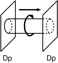
Figure 2.1: Open-closed duality

Before solving this constraint equation we have to notice that the closed string Hilbert space which is spanned by boundary states are only limited to NSNS and RR-sector. The proof of this is as follows. First, if we consider the open string picture in figure 2.1, we can see that open strings should have some kind of periodicity in the direction of the worldsheet time $\sigma_{2}$ because the cylinder represents an open string one loop diagram. If we set this periodicity to $T$, this statement can be represented by

$$\left\{\begin{array}[]{c}\psi^{\mu}_{L}(\sigma_{1},0)=\gamma_{3}\psi^{\mu}_{L}(\sigma_{1},T),\\ \psi^{\mu}_{R}(\sigma_{1},0)=\gamma_{4}\psi^{\mu}_{R}(\sigma_{1},T).\end{array}\right.$$ (2.1.6)

Here the periodicity of bosonic fields $X^{\mu}(\sigma_{1},\sigma_{2})$ is irrelevant in this proof, thus we have omitted it. By using the above relations we can prove the following identities:

$$\psi^{\mu}_{L}(0,0)\mathop{=}_{(\ref{cylperiod})}\gamma_{3}\psi^{\mu}_{L}(0,T)\mathop{=}_{(\ref{bc1})}\gamma_{3}\gamma_{1}S^{\mu}_{~{}\nu}\psi^{\nu}_{R}(0,T),$$ (2.1.7)

and

$$\psi^{\mu}_{L}(0,0)\mathop{=}_{(\ref{bc1})}\gamma_{1}S^{\mu}_{~{}\nu}\psi^{\nu}_{R}(0,T)\mathop{=}_{(\ref{cylperiod})}\gamma_{1}\gamma_{4}S^{\mu}_{~{}\nu}\psi^{\nu}_{R}(0,T).$$ (2.1.8)

From these equations the following relation holds:

$$\gamma_{3}=\gamma_{4}.$$ (2.1.9)

If we see figure 2.1 in the closed string picture, equation (2.1.6) can be regarded as the boundary condition of closed strings emitted by the D$p$-brane. It indicates that there is no NS-R or R-NS sector in the boundary state.

Now we have come to the stage of solving constraint equation (2.1). By inserting mode expansions of $X^{\mu},\psi^{\mu}_{L}$ and $\psi^{\mu}_{R}$ (see eq.(A.1)) into eq.(2.1) we can obtain the following equations:

$$(\alpha^{\mu}_{m}+S^{\mu}_{~{}\nu}\tilde{\alpha}_{-m}^{\nu})|Dp,\gamma\rangle_{\scriptscriptstyle NSNS(RR)}=0,$$ (2.1.10)

$$(\psi^{\mu}_{r}-i\gamma S^{\mu}_{~{}\nu}\tilde{\psi}^{\nu}_{-r})|Dp,\gamma\rangle_{\scriptscriptstyle NSNS(RR)}=0,$$ (2.1.11)

where we have rewritten $\gamma_{1}$ with $\gamma$ and the value of the subscript label $r$ takes half-integers(integers) for NSNS(RR)-sector.

For nonzero modes

     For nonzero modes ($\alpha^{\mu}_{m},~{}\psi^{\mu}_{r},~{}\tilde{\psi}^{\mu}_{r}~{}(m,r\neq 0)$) the above equations can be easily solved and the result is equal to the following coherent state:

$$|Dp,\gamma\rangle_{\scriptscriptstyle NSNS(RR)} = {\cal N}_{p}\exp\left[-\sum^{\infty}_{m=1}m^{-1}\alpha^{\mu}_{-m}S_{\mu\nu}\tilde{\alpha}^{\nu}_{-m}+i\gamma\sum_{r>0}\psi^{\mu}_{-r}S_{\mu\nu}\tilde{\psi}^{\nu}_{-r}\right]$$ (2.1.12)

$$~{}~{}~{}~{}~{}~{}~{}~{}~{}~{}~{}~{}~{}~{}~{}~{}~{}~{}~{}~{}~{}~{}~{}~{}~{}~{}~{}~{}~{}~{}~{}~{}~{}~{}~{}~{}~{}~{}~{}\times~{}|Dp,\gamma\rangle^{0}_{\scriptscriptstyle NSNS(RR)},$$

where $|Dp,\gamma\rangle^{0}_{\scriptscriptstyle NSNS(RR)}$ is the contribution from zero modes including the conformally invariant vacuum $|0\rangle$, and ${\cal N}_{p}$ is the normalization constant of $|Dp,\gamma\rangle_{\scriptscriptstyle NSNS(RR)}$, which can be determined by Cardy’s condition [54] explained later.

For zero modes

     Equations (2.1.10) and (2.1.11) for zero modes are rewritten as

$$(p^{\alpha}_{L}+p^{\alpha}_{R})|Dp,\gamma\rangle^{0}_{\scriptscriptstyle NSNS(RR)} = 0,~{}~{}~{}~{}~{}(p^{i}_{L}-p^{i}_{R})|Dp,\gamma\rangle^{0}_{\scriptscriptstyle NSNS(RR)}=0,$$ (2.1.13)

$$(\psi^{\alpha}_{0}-i\gamma\tilde{\psi}^{\alpha}_{0})|Dp,\gamma\rangle^{0}_{\scriptscriptstyle RR} = 0,~{}~{}~{}~{}~{}(\psi^{i}_{0}+i\gamma\tilde{\psi}^{i}_{0})|Dp,\gamma\rangle^{0}_{\scriptscriptstyle RR}=0,$$ (2.1.14)

where $\alpha,\beta,\cdots=0,\cdots,p$ and $i,j,\cdots=p+1,\cdots,9$. Note that equations (2.1.14) are defined only in RR-sector of the boundary state.

For equations (2.1.13) the solution depends on whether we consider a non-compactified direction or a compactified direction. For a non-compactified direction the second equation in eq.(2.1.13) becomes a trivial equation and the first equation in eq.(2.1.13) can be rewritten as $p^{\alpha}|Dp,\gamma\rangle^{0}_{\scriptscriptstyle NSNS(RR)}=0$. Moreover if the position of the D$p$-brane is $x^{i}=a^{i}$, the Hilbert space for zero modes can be written as

$$\delta^{9-p}(x^{i}-a^{i})|0\rangle=\int\frac{d^{9-p}k}{(2\pi)^{9-p}}e^{ik_{i}(x-a)^{i}}|0\rangle\equiv\int\frac{d^{9-p}k}{(2\pi)^{9-p}}e^{-ik_{i}a^{i}}|{\bf 0},{\bf k}\rangle,$$ (2.1.15)

where

$$\langle{\bf 0},{\bf k}|{\bf 0},{\bf k}^{\prime}\rangle=(2\pi)^{9-p}\delta^{9-p}({\bf k-k}^{\prime}).$$ (2.1.16)

Note that this state satisfies $p^{\alpha}|Dp,\gamma\rangle^{0}_{\scriptscriptstyle NSNS(RR)}=0$.

For a compactified direction the equations in eq.(2.1.13) can be rewritten as

$$n^{\alpha}|Dp,\gamma\rangle^{0}_{\scriptscriptstyle NSNS(RR)} = 0,$$

$$w^{i}|Dp,\gamma\rangle^{0}_{\scriptscriptstyle NSNS(RR)} = 0,$$ (2.1.17)

where $n^{\alpha}$ and $w^{i}$ denote the momentum number and the winding number (see eq.(A.1)). If we consider the ten-dimensional space where all of the directions are compactified, the Hilbert space of this state can be spanned by the linear combination of $|{\bf w},{\bf n}\rangle$ such as ${\displaystyle\sum_{w^{\alpha}\in{\bf Z}^{p+1},n^{i}\in{\bf Z}^{9-p}}f_{{\bf w},{\bf n}}|{\bf w},{\bf n}\rangle}$, where $f_{{\bf w},{\bf n}}$ is an coefficient for a given sector with $w^{\alpha},n^{i}$. To determine it we make eq.(2.1.15) discrete like

$$\int\frac{d^{9-p}k}{(2\pi)^{9-p}}e^{ik_{i}(x-a)^{i}}|0\rangle \rightarrow (V_{9-p})^{-1}\sum_{n^{i}\in{\bf Z}^{9-p}}e^{i\frac{n^{i}}{R_{i}}(x-a)^{i}}|0\rangle$$ (2.1.18)

$$\equiv ~{}(V_{9-p})^{-1}\sum_{n^{i}\in{\bf Z}^{9-p}}e^{-i\frac{n^{i}}{R_{i}}a^{i}}|{\bf 0},{\bf n}\rangle.$$

Corresponding to the last equation we can consider a state with winding numbers given by

$$\sum_{w^{\alpha}\in{\bf Z}^{p+1}}e^{i\frac{w^{\alpha}R_{\alpha}}{2}(x^{\alpha}_{L}-x^{\alpha}_{R}-a^{\alpha})}|0\rangle~{}\equiv~{}\sum_{w^{\alpha}\in{\bf Z}^{p+1}}e^{-i\frac{w^{\alpha}R_{\alpha}}{2}a^{\alpha}}|{\bf w},{\bf 0}\rangle,$$ (2.1.19)

where $a^{\alpha}$ is called the Wilson line. By T-duality ($R\leftrightarrow\frac{2}{R},~{}n\leftrightarrow w$) this corresponds to the parameter $a^{i}$ in eq.(2.1.18), which represents the position of the D$p$-brane. In terms of open strings these parameters $a^{\alpha}$ and $a^{i}$ can be interpreted as expectation values of open string backgrounds $A^{\alpha}(X(z,\bar{z}))~{}(\mbox{gauge field})$ and $\Phi^{i}(X(z,\bar{z}))~{}(\mbox{transverse scalar})$.

After all in compactified directions the zero mode part of boundary states can be written as

$$(V_{9-p})^{-1}\sum_{w^{\alpha}\in{\bf Z}^{p+1},n^{i}\in{\bf Z}^{9-p}}e^{-i\left(\frac{w^{\alpha}R_{\alpha}}{2}a^{\alpha}+\frac{n^{i}}{R_{i}}a^{i}\right)}|{\bf w},{\bf n}\rangle.$$ (2.1.20)

Corresponding to (2.1.16) the normalization of $|{\bf n},{\bf w}\rangle$ becomes

$$\langle{\bf n}^{\prime},{\bf w}^{\prime}|{\bf n},{\bf w}\rangle=V\delta_{{\bf n}^{\prime},{\bf n}}\delta_{{\bf w}^{\prime},{\bf w}},$$ (2.1.21)

where $V$ is the volume of the compactified space.

The equation left to solve is eq.(2.1.14), which determines the contribution from zero modes of worldsheet fermions $\psi^{\mu}_{L}$ and $\psi^{\mu}_{R}$ in the RR-sector. To solve this we first define the following new valuables:

$$\psi^{\mu}_{\pm}=\frac{1}{\sqrt{2}}(\psi^{\mu}_{0}\pm i\tilde{\psi}^{\mu}_{0}),$$ (2.1.22)

and also define $|\Omega p,\gamma\rangle^{0}_{\scriptscriptstyle RR}$ as the limited Hilbert space of $|Dp,\gamma\rangle^{0}_{\scriptscriptstyle RR}$ which is spanned only by $\psi^{\mu}_{0}$ and $\tilde{\psi}^{\mu}_{0}$. By using these we can rewritten eq.(2.1.14) simply as

$$\psi^{\alpha}_{-}|\Omega p,+\rangle^{0}_{\scriptscriptstyle RR}=0~{} ~{}\psi^{i}_{+}|\Omega p,+\rangle^{0}_{\scriptscriptstyle RR}=0~{},$$ ,

$$\psi^{\alpha}_{+}|\Omega p,-\rangle^{0}_{\scriptscriptstyle RR}=0~{} ~{}\psi^{i}_{-}|\Omega p,-\rangle^{0}_{\scriptscriptstyle RR}=0.$$ , (2.1.23)

Since we can obtain the anticommuting relations between these valuables as

$$\{\psi^{\mu}_{\pm},\psi^{\nu}_{\pm}\}=0~{},~{}\{\psi^{\mu}_{+},\psi^{\nu}_{-}\}=\eta^{\mu\nu},$$ (2.1.24)

we can construct the zero mode part of boundary states by using the representation theory of Clifford Algebra.

First we can define “the ground state” $|\Omega\rangle^{0}_{\scriptscriptstyle RR}$ as $|\Omega\rangle^{0}_{\scriptscriptstyle RR}\equiv|\Omega 7,+\rangle^{0}_{\scriptscriptstyle RR}$ because of
$\psi^{\mu}_{-}|\Omega 7,+\rangle^{0}_{\scriptscriptstyle RR}=0$ for all $\mu~{}(\mu=-1,0,\cdots,7)$. Next we can define “the excited states” by multiplying creation operators $\psi^{\mu}_{+}$ by this ground state. Especially the state which satisfies eq.(2.1) is given by

$$|\Omega p,+\rangle^{0}_{\scriptscriptstyle RR}=\prod_{i}\psi^{i}_{+}|\Omega\rangle^{0}_{\scriptscriptstyle RR},$$

$$|\Omega p,-\rangle^{0}_{\scriptscriptstyle RR}=\prod_{\alpha}\psi^{\alpha}_{+}|\Omega\rangle^{0}_{\scriptscriptstyle RR}.$$ (2.1.25)

The ambiguity left in this solution is phase factors $\pm 1$ and the normalization of “the ground state” $|\Omega\rangle^{0}_{\scriptscriptstyle RR}$. The first ambiguity can be gotten rid of by fixing the convention. Here we have chosen the following convention:

$$|\Omega p,+\rangle^{0}_{\scriptscriptstyle RR} = \psi^{7}_{+}\psi^{6}_{+}\cdots\psi^{p+1}_{+}|\Omega\rangle^{0}_{\scriptscriptstyle RR},$$

$$|\Omega p,-\rangle^{0}_{\scriptscriptstyle RR} = \psi^{0}_{+}\psi^{1}_{+}\cdots\psi^{p}_{+}|\Omega\rangle^{0}_{\scriptscriptstyle RR},$$ (2.1.26)

for a D$p$-brane which extends in directions $X^{0},X^{1},\cdots X^{p}$. The second ambiguity is not related to the convention. The method to fix this is the same as that of fixing the total normalization ${\cal N}_{p}$ in eq.(2.1.12). Here, to avoid the complicated situation we first give the answer to this:

$$\langle\Omega|\Omega\rangle^{0}_{\scriptscriptstyle RR}=16.$$ (2.1.27)

You can check that this result is consistent with the later calculation of the interaction between two D$p$-branes. By using this the normalization of the zero mode part $|Dp,\gamma\rangle^{0}_{\scriptscriptstyle RR}$ can be calculated and the result is

$$\langle\Omega p,\gamma|\Omega p,\gamma^{\prime}\rangle^{0}_{\scriptscriptstyle RR}=16\delta_{\gamma,\gamma^{\prime}}.$$ (2.1.28)

GSO projection in the NSNS-sector

     To obtain the modular invariant spectrum in closed string theory we have to perform GSO-projection. This can be applied to boundary states too because these states also belong to the closed string Hilbert space. In the NSNS sector the worldsheet fermion number $F$ is defined by

$$F=\sum^{\infty}_{r=1/2}\psi^{\mu}_{-r}\psi_{\mu r}-1,$$ (2.1.29)

and $\tilde{F}$ is defined by replacing $\psi_{r}$ with $\tilde{\psi}_{r}$. By a simple calculation we can see the relations

$$(-1)^{F}|Dp,\gamma\rangle_{\scriptscriptstyle NSNS}=-|Dp,-\gamma\rangle_{\scriptscriptstyle NSNS},$$

$$(-1)^{\tilde{F}}|Dp,\gamma\rangle_{\scriptscriptstyle NSNS}=-|Dp,-\gamma\rangle_{\scriptscriptstyle NSNS},$$ (2.1.30)

where we have included the ghost contribution in the fermion number.

Therefore we can obtain the following linearly combined boundary state which is GSO-invariant $\left((-1)^{F}=1,~{}(-1)^{\tilde{F}}=1\right)$ in the NSNS-sector

$$|Dp\rangle_{\scriptscriptstyle NSNS}=\frac{1}{2}(|Dp,+\rangle_{\scriptscriptstyle NSNS}-|Dp,-\rangle_{\scriptscriptstyle NSNS}),$$ (2.1.31)

where we have included $\frac{1}{2}$ for later convenience.

GSO projection in the RR-sector

     In the RR-sector the worldsheet fermion number $F$ is defined by

$$(-1)^{F}~{}\equiv~{}2^{4}\psi^{0}_{0}\cdots\psi^{7}_{0}(-1)^{\sum^{\infty}_{m=1}\psi^{\mu}_{-m}\psi_{\mu m}}.$$ (2.1.32)

By using eq.(2.1.12) and (2.1) we can obtain the following relations

$$(-1)^{F}|Dp,\gamma\rangle_{\scriptscriptstyle RR}=|Dp,-\gamma\rangle_{\scriptscriptstyle RR},$$

$$~{}(-1)^{\tilde{F}}|Dp,\gamma\rangle_{\scriptscriptstyle RR}=(-1)^{7-p}|Dp,-\gamma\rangle_{\scriptscriptstyle RR},$$ (2.1.33)

where the phase factor $(-1)^{7-p}$ comes from the zero mode contribution. From the first equation we can see that the GSO-invariant state in the left-sector $((-1)^{F}=1)$ is

$$|Dp\rangle_{\scriptscriptstyle RR}=\frac{1}{2}(|Dp,+\rangle_{\scriptscriptstyle RR}+|Dp,-\rangle_{\scriptscriptstyle RR}).$$ (2.1.34)

This state also has to satisfy the GSO-projection in the right-sector
$((-1)^{\tilde{F}}=\mp 1~{}~{}(-1~{}\mbox{for IIA},~{}+1~{}\mbox{for IIB}))$. From this constraint we can see the correct spectrum of D$p$-branes with even(odd) integer $p$ for IIA(IIB).


Normalization of the boundary state

     At this stage we have the complete form of boundary state $|Dp\rangle$ written by

$$|Dp\rangle~{}\equiv~{}|Dp\rangle_{\scriptscriptstyle NSNS}+|Dp\rangle_{\scriptscriptstyle RR},$$ (2.1.35)

where $|Dp\rangle_{\scriptscriptstyle NSNS}$ and $|Dp\rangle_{\scriptscriptstyle RR}$ are defined in eq.(2.1.31) and eq.(2.1.34), while we have not yet determined the normalization constant ${\cal N}_{p}$, which appears in eq.(2.1.12). This constant can be determined by the consistency (“Cardy Condition” [54]) which comes from open-closed duality in figure 2.1.

First we can see that figure 2.1 can be regarded as a diagram of interaction between two parallel D$p$-branes. It is represented by ${\cal A}=\langle Dp|\Delta|Dp\rangle$, where $\Delta$ is a closed string propagator

$$\Delta = \frac{1}{2\pi}\int_{|z|\leq 1}\frac{d^{2}z}{|z|^{2}}z^{L_{0}}\bar{z}^{\tilde{L}_{0}}$$ (2.1.36)

$$\rightarrow \int^{\infty}_{0}ds\exp[-s(L_{0}+\tilde{L}_{0})].$$

Here we have used the relation $(L_{0}-\tilde{L}_{0})|Dp\rangle=0$, which we can easily check from the explicit expression of $L_{0}$ and $\tilde{L}_{0}$ (see eq.(A.1.4)). The explicit form of this amplitude can easily be calculated and its result becomes

$${\cal A} = \frac{1}{2}|{\cal N}_{p}|^{2}V_{p+1}\int^{\infty}_{0}ds(4\pi s)^{-\frac{9-p}{2}}\left[\frac{f_{3}(q)^{8}-f_{4}(q)^{8}-f_{2}(q)^{8}}{f_{1}(q)^{8}}\right]$$ (2.1.37)

$$= 0,$$

where $V_{p+1}$ denotes the (p+1)-dimensional volume, and we have used modular functions $f_{i}(q)~{}(i=1,2,3,4)$ defined by

$$f_{1}(q)=q^{\frac{1}{12}}\prod_{n=1}^{\infty}(1-q^{2n}) f_{2}(q)=\sqrt{2}q^{\frac{1}{12}}\prod_{n=1}^{\infty}(1+q^{2n}),$$ ,

$$f_{3}(q)=q^{-\frac{1}{24}}\prod_{n=1}^{\infty}(1+q^{2n-1}) f_{4}(q)=q^{-\frac{1}{24}}\prod_{n=1}^{\infty}(1-q^{2n-1}),$$ , (2.1.38)

with $q=e^{-s}$. In the second line of eq.(2.1.37) we have used the famous Jacobi’s abstruse identity:

$$f_{3}(q)^{8}-f_{2}(q)^{8}-f_{4}(q)^{8}=0,$$ (2.1.39)

and this result represents the fact that the force between two parallel D-branes is zero and D-branes are stable. In other words the gravitational attractive force from the NSNS-sector exactly cancels the repulsive Coulomb force from the RR-sector.

On the other hand we can see that figure 2.1 can be regarded as an one-loop diagram of open strings. The partition function (cylinder amplitude) of this diagram is represented by

$${\cal Z}_{{\scriptscriptstyle C}_{2}}=V_{p+1}\int^{\infty}_{0}\frac{dt}{2t}{\rm Tr}_{\scriptscriptstyle NS-R}\left[\frac{1+(-1)^{F}}{2}\tilde{q}^{2L_{0}}\right],$$ (2.1.40)

where ${\rm Tr}_{\scriptscriptstyle NS-R}\equiv{\rm Tr}_{\scriptscriptstyle NS}-{\rm Tr}_{\scriptscriptstyle R}$ and $\tilde{q}=e^{-\pi t}$. its explicit result is given by

$${\cal Z}_{{\scriptscriptstyle C}_{2}} = 2V_{p+1}\int^{\infty}_{0}\frac{dt}{4t}(16\pi^{2}t)^{-\frac{p+1}{2}}\left[\frac{f_{3}(\tilde{q})^{8}-f_{4}(\tilde{q})^{8}-f_{2}(\tilde{q})^{8}}{f_{1}(\tilde{q})^{8}}\right]$$ (2.1.41)

$$= \frac{1}{2}V_{p+1}(16\pi^{2})^{-\frac{p+1}{2}}\pi^{\frac{7-p}{2}}\int^{\infty}_{0}~{}ds~{}s^{-\frac{9-p}{2}}\left[\frac{f_{3}(q)^{8}-f_{2}(q)^{8}-f_{4}(q)^{8}}{f_{1}(q)^{8}}\right]$$

$$= 0,$$

where the extra factor $2$ in the first line comes from the Chan-Paton factor. In the second line we have used coordinate transformation with $s=\frac{\pi}{t}$ and modular properties of modular functions $f_{i}(q)$ given by

$$f_{1}(e^{-\frac{\pi}{t}})=\sqrt{t}f_{1}(e^{-\pi t}) f_{2}(e^{-\frac{\pi}{t}})=f_{4}(e^{-\pi t}),$$ ,

$$f_{3}(e^{-\frac{\pi}{t}})=f_{3}(e^{-\pi t}) f_{4}(e^{-\frac{\pi}{t}})=f_{2}(e^{-\pi t}).$$ , (2.1.42)

The third line in eq.(2.1.41) comes from Jacobi’s abstruse identity (2.1.39), and this result represents the fact that there are some target space supersymmetries left.

If we compare this result (2.1.41) with eq.(2.1.37) we can determine the coefficient ${\cal N}_{p}$ of the boundary state, which is given by

$${\cal N}_{p}=\frac{\sqrt{\pi}(2\sqrt{2}\pi)^{3-p}}{2}\equiv\frac{T_{p}}{2}.$$ (2.1.43)

Here we can see that $\kappa^{-1}T_{p}$ is equal to the tension of a D$p$-brane ($\kappa$ is the ten dimensional gravitational constant).

2.2 Generalized Boundary State

In the previous section we have defined the boundary states which describe various D$p$-branes. In this section we will extend these boundary states into more general ones [55, 56]. To explain this let us consider an example of a quantum mechanical amplitude which is given by

$$\langle\beta|e^{-HT}|\alpha\rangle,$$ (2.2.44)

where $H$ is the Hamiltonian of the system of harmonic oscillators, and $|\alpha\rangle$ and $|\beta\rangle$ correspond to the states in the Schroedinger picture which represent some boundary conditions at $t=0$ and $t=T$. This is an transition amplitude from $|\alpha\rangle$ to $|\beta\rangle$.

On the other hand if we re-express this amplitude by using the path-integral formalism, it becomes

$$\int{\cal D}q~{}e^{-\int^{T}_{0}dt{\cal L}(q(t))}e^{-I_{\beta}(q(T))}e^{-I_{\alpha}(q(0))},$$ (2.2.45)

where $q(t)$ and ${\cal L}(q)$ are the variable and its Lagrangian which describe the system of harmonic oscillators. What we would like to note here is that there appear boundary terms $e^{-I_{\beta}(q(T))}$ and $e^{-I_{\alpha}(q(0))}$ in the path-integral. These factors come from the internal products

$$\langle q|\alpha\rangle=e^{-I_{\alpha}(q)},$$ (2.2.46)

where $|q\rangle$ is the coherent state defined by

$$\hat{q}|q\rangle=q|q\rangle.$$ (2.2.47)

The most important feature of the coherent state is that this satisfies the completeness condition which is represented by

$$\int{\cal D}q~{}|q\rangle\langle q|=1.$$ (2.2.48)

Because of this fact we can expand any quantum mechanical state by using the coherent state. Especially the state $|\alpha\rangle$ can be expressed in the following way:

$$|\alpha\rangle=\int{\cal D}q~{}e^{-I_{\alpha}(q)}|q\rangle.$$ (2.2.49)

This is the one-dimensional example of the generalized state when we assign the weight $e^{-I_{\alpha}(q)}$ to the boundary ($t=0)$.

Now we would like to extend this formalism to that for string theory. First of all we will define the coherent state $|x,\varphi\rangle_{\scriptscriptstyle NSNS(RR)}$ as the two-dimensional extension of the state (2.2.47). Its definition in the NSNS-sector is the direct product of $|x\rangle$ and $|\varphi\rangle_{\scriptscriptstyle NSNS}=\frac{1}{2}\left(|\varphi,+\rangle_{\scriptscriptstyle NSNS}-|\varphi,-\rangle_{\scriptscriptstyle NSNS}\right)$ which are defined by

$$X^{\mu}(\sigma_{1},0)|x\rangle = x^{\mu}(\sigma_{1})|x\rangle,$$

$$\left(\psi^{\mu}_{L}(\sigma_{1},0)+i\gamma\psi^{\mu}_{R}(\sigma_{1},0)\right)|\varphi,\gamma\rangle_{\scriptscriptstyle NSNS} = \varphi^{\mu}(\sigma_{1})|\varphi,\gamma\rangle_{\scriptscriptstyle NSNS}~{}~{}~{}~{}~{}(\gamma=\pm 1),$$ (2.2.50)

where

$$x^{\mu}(\sigma_{1}) = ~{}\sum_{m\in{\bf Z}}~{}x^{\mu}_{m}e^{im\sigma_{1}},$$

$$\varphi^{\mu}(\sigma_{1}) = \sum_{r\in{\bf Z}+1/2}\varphi^{\mu}_{r}e^{ir\sigma_{1}}.$$ (2.2.51)

The way to solve these equation is almost the same as in the previous section. The answer is given by

$$|x\rangle = \exp\left[\sum^{\infty}_{m=1}\left\{-\frac{m}{2}x^{\mu}_{-m}x_{m\mu}+\frac{1}{m}\alpha^{\mu}_{-m}\tilde{\alpha}_{-m\mu}-\alpha^{\mu}_{-m}x_{m\mu}+x^{\mu}_{-m}\tilde{\alpha}_{-m\mu}\right\}\right]|0\rangle,$$

$$|\varphi,\gamma\rangle_{\scriptscriptstyle NSNS} = \exp\left[\sum^{\infty}_{r=1/2}\left\{-\frac{1}{2}\varphi^{\mu}_{-r}\varphi_{r\mu}-i\gamma\psi^{\mu}_{-r}\tilde{\psi}_{-r\mu}+\psi^{\mu}_{-r}\varphi_{r\mu}+i\gamma\varphi^{\mu}_{-r}\tilde{\psi}_{-r\mu}\right\}\right]|0\rangle.$$

Here we have defined the total normalization to satisfy the completeness condition

$$\begin{array}[]{c}{\displaystyle\int{\cal D}x|x\rangle\langle x|=1},\\ {\displaystyle\int{\cal D}\varphi|\varphi,\gamma\rangle_{\scriptscriptstyle NSNS}\langle\varphi,\gamma|_{\scriptscriptstyle NSNS}=1.}\end{array}$$ (2.2.53)

This is the result for the NSNS-sector, while we can define this kind of state in the RR-sector in the similar way.

Because of this completeness condition we can expand any boundary states in the following way

$$|B~{}\rangle_{\scriptscriptstyle NSNS(RR)}=\int{\cal D}x{\cal D}\varphi~{}e^{-I_{B}(x,\varphi)}|x,\varphi\rangle_{\scriptscriptstyle NSNS(RR)},$$ (2.2.54)

where $e^{-I_{B}(x,\varphi)}$ is the wave function corresponding to some boundary condition. If we use the definition of $|x,\varphi\rangle_{\scriptscriptstyle NSNS(RR)}$ in eq.(2.2) we can also rewritten the above equation as

$$|B~{}\rangle_{\scriptscriptstyle NSNS(RR)} = \frac{1}{2}\exp\left[-I_{B}\left(X,\psi_{L}+i\psi_{R}\right)\right]\int{\cal D}x{\cal D}\varphi~{}|x,\varphi,+\rangle_{\scriptscriptstyle NSNS(RR)}$$ (2.2.55)

$$~{}~{}~{}~{}~{}~{}\mp\frac{1}{2}\exp\left[-I_{B}\left(X,\psi_{L}-i\psi_{R}\right)\right]\int{\cal D}x{\cal D}\varphi~{}|x,\varphi,-\rangle_{\scriptscriptstyle NSNS(RR)}$$

$$= \frac{1}{2}\exp\left[-I_{B}\left(X,\psi_{L}+i\psi_{R}\right)\right]|D9,+\rangle_{\scriptscriptstyle NSNS(RR)}$$

$$~{}~{}~{}~{}~{}~{}\mp\frac{1}{2}\exp\left[-I_{B}\left(X,\psi_{L}-i\psi_{R}\right)\right]|D9,-\rangle_{\scriptscriptstyle NSNS(RR)},$$

where $|D9~{},\pm\rangle_{\scriptscriptstyle NSNS}$ is the boundary state for a D9-brane defined in eq.(2.1.12), and $X^{\mu}$ and $\psi^{\mu}_{L(R)}$ act on the boundary state as operators. If we set $I_{B}(x,\varphi)$ to zero, this boundary state is proportional to $|D9~{}\rangle_{\scriptscriptstyle NSNS(RR)}$. If we would like to consider the boundary state for a D$p$-brane, we have only to perform the T-duality transformation.

In general we can identify $I_{B}(x,\varphi)$ as some boundary action on the disk like

$$I_{B}(x,\varphi) = \int^{\pi}_{-\pi}d\sigma_{1}d\theta~{}D_{\theta}{\bf X}^{\mu}A_{\mu}({\bf X})$$ (2.2.56)

$$= \int^{\pi}_{-\pi}d\sigma_{1}\left[-i\frac{\partial x^{\mu}}{\partial\sigma_{1}}A_{\mu}(x)+\frac{1}{2}\varphi^{\mu}\varphi^{\nu}F_{\mu\nu}(x)\right],$$

where

$$\left\{\begin{array}[]{lcl}{\bf X}^{\mu}&=&x^{\mu}+i\theta\varphi^{\mu},\\ D_{\theta}&=&\frac{\partial}{\partial\theta}+i\theta\frac{\partial}{\partial\sigma_{1}}.\end{array}\right.$$ (2.2.59)

If the gauge field $A_{\mu}(x)$ satisfies its equation of motion, the boundary state (2.2.54) represents a BPS D9-brane with the external gauge field on it. In this case the conformal invariance in the worldsheet is preserved.

In chapter 3 and 4 we will assign more general actions to $I_{B}(x,\varphi)$ in eq.(2.2.54) or eq.(2.2.55). Especially in chapter 3 we will start with the action which does not satisfy the conformal invariance. In this way we can generalize the usual boundary conditions for D-branes into more general ones.

2.3 The Definition of Non-BPS Systems

In the previous section we have defined the familiar BPS D-branes by using the boundary state formalism. The characteristic property of these D-branes is the fact that these are supersymmetric and stable. On the other hand we can also define unstable D-brane systems in Type II string theories. The perturbative instability of these D-branes indicates that these systems are nonsupersymmetric and decay to something stable. It is important to study the unstable non-BPS systems because the decay of these unstable D-brane systems can be considered as one of dynamical processes in string theory, which have not been studied and have not figured out for years. Therefore in this section we will define the non-BPS D-brane systems by using the boundary state method.

2.3.1 The brane-antibrane system

The important non-BPS systems consist of two kinds of D-brane systems. These are called the brane-antibrane system and the non-BPS D-branes. First we will explain the brane-antibrane system. The antibrane is defined by a D-brane which has the opposite RR-charge to an usual D-brane. The boundary state of this kind of D$p$-branes is written by

$$|\overline{Dp}\rangle~{}\equiv~{}|Dp\rangle_{\scriptscriptstyle NSNS}-|Dp\rangle_{\scriptscriptstyle RR}.$$ (2.3.60)

If we compare this boundary state with eq.(2.1.35), we can see that the sign in front of the RR-sector is opposite to that in eq.(2.1.35). We can easily see that this D$p$-brane has the opposite RR-charge if we compute the coupling with a (p+1)-form RR-gauge field $C_{p+1}$, which is given by $\langle C_{p+1}|\overline{Dp}\rangle$.

The important thing here is to consider a D-brane and an anti D-brane at the same time. If we put these two kinds of D$p$-branes in the parallel position, the only attractive force remains between these D$p$-branes, because not only the gravitational force but also the Coulomb force is attractive [57]. We can check this fact quantitatively by using the boundary state method. As we saw in eq.(2.1.37) the interaction is represented by $\langle\overline{Dp}|\Delta|Dp\rangle$, and its explicit result is

$$\langle\overline{Dp}|\Delta|Dp\rangle = \frac{T_{p}^{2}}{8}V_{p+1}\int^{\infty}_{0}ds(4\pi s)^{-\frac{9-p}{2}}\left[\frac{f_{3}(q)^{8}-f_{4}(q)^{8}+f_{2}(q)^{8}}{f_{1}(q)^{8}}\right],$$ (2.3.61)

with $q=e^{-s}$. In this result the sign in front of $f_{2}(q)$ is opposite to that in eq.(2.1.37), thus this amplitude is not zero and indicates that this system is unstable. Moreover, if we perform the coordinate transformation $s=\frac{\pi}{t}$ and use the modular properties (2.1) of functions $f_{i}(q)$, we can find that this equation can be rewritten in the form of partition function of open strings as

$$V_{p+1}\int^{\infty}_{0}\frac{dt}{2t}{\rm Tr}_{\scriptscriptstyle NS-R}\left[\frac{1-(-1)^{F}}{2}\tilde{q}^{2L_{0}}\right]~{}~{}~{}(\tilde{q}=e^{-\pi t}).$$ (2.3.62)

Here note that the sign in front of $(-1)^{F}$ is minus. This fact indicates that open strings between a D$p$-brane and an anti D$p$-brane obey the opposite GSO projection, which leaves an open string tachyon in the spectrum. If we admit the fact that the tachyon signals instability of the system, we can consider that this system decays to something.

Finally note that the total tension and total mass of a brane-antibrane system is modified by quantum corrections. The classical tension of a brane-antibrane is given by $\frac{2T_{p}}{\kappa}=\frac{2\tau_{p}}{g}$, where $g$ is the string coupling constant and $\tau_{p}$ is given by

$$\tau_{p}=\frac{1}{\sqrt{2}(2\sqrt{2}\pi)^{p}}.$$ (2.3.63)

If we consider the quantum theory, the tension is modified as

$$\frac{2\tau_{p}}{g}+a_{0}+a_{1}g+a_{2}g^{2}+\cdots\cdots,$$ (2.3.64)

where $a_{0},a_{1},\cdots$ represent unknown constants. On the other hand the tension and the mass of a BPS D-brane is not modified by quantum corrections due to the target space supersymmetry.

2.3.2 The non-BPS D-brane

We can define the other unstable system which is called the non-BPS D-brane. It is easy to define this D-brane by using the boundary state too. The boundary state for a non-BPS D$p$-brane is defined by

$$|NDp\rangle~{}\equiv~{}\sqrt{2}|Dp\rangle_{\scriptscriptstyle NSNS}.$$ (2.3.65)

Note that the RR-sector of the boundary state does not exist and that the coefficient $\sqrt{2}$ appears. The first fact indicates that non-BPS D-branes do not have any RR-charges because the coupling with a (p+1)-form RR-gauge field $\langle C_{p+1}|NDp\rangle$ is equal to zero. The second fact means that the tension of a non-BPS D$p$-brane is $\sqrt{2}$ times as large as that of a BPS D$p$-brane. We can easily verify this by calculating the coupling $\langle 0|NDp\rangle$ with the vacuum.

The latter fact stems from Cardy’s condition [54]. If we calculate the interaction $\langle NDp|\Delta|NDp\rangle$ between two non-BPS D$p$-branes and transform it to the open string partition function, it becomes

$$V_{p+1}\int^{\infty}_{0}\frac{dt}{2t}{\rm Tr}_{\scriptscriptstyle NS-R}\tilde{q}^{2L_{0}}~{}~{}~{}(\tilde{q}=e^{-\pi t}).$$ (2.3.66)

This is just the partition function without GSO projection. If we remove the $\sqrt{2}$ factor from the boundary state (2.3.65), its partition function becomes half of eq.(2.3.66), and this is inconsistent with the open string theory. Therefore, we have to include $\sqrt{2}$ factor in the boundary state.

The important point about non-BPS D-branes is that there exists a tachyon in the open string spectrum, which can be seen from eq.(2.3.66). In the same way as the brane-antibrane system, this is the signal that non-BPS D-branes are unstable and decay to something stable.

Now we have to notice that not all kinds of non-BPS D$p$-branes can exist in Type IIA(B) theory. In fact, in Type IIA theory non-BPS D$p$-branes with only odd integer $p$ can exist, while in Type IIB theory those with only even integer $p$ can. This is complementary to the fact that in Type IIA(B) there exist BPS D$p$-branes with even(odd) integer $p$. Its proof is simple. First we suppose that a BPS D$p$-brane and a non-BPS D$p$-brane could exist at the same time. Next we calculate the interaction between them and transform it into the form of partition function of open strings. The result is equal to $\frac{1}{\sqrt{2}}$ times as large as eq.(2.3.66) and is not a consistent one as we said.

Finally note that the tension of a non-BPS D-brane is also modified by quantum corrections in the same way as eq.(2.3.64).

2.3.3 The Chan-Paton factors and $(-1)^{F^{\scriptscriptstyle S}_{\scriptscriptstyle L}}$ twist

Here we add Chan-Paton degrees of freedom to open strings on two kinds of non-BPS systems. For example, to describe the complete Hilbert space of open strings in a pair of brane and antibrane, we should prepare all two-by-two matrices which are spanned by an unit element and three Pauli matrices $\{1,\sigma_{1},\sigma_{2},\sigma_{3}\}$. To obtain the correct spectrum of all kinds of open strings on a pair of brane and antibrane, we attach the fermion number $\{+,-,-,+\}$ to $\{1,\sigma_{1},\sigma_{2},\sigma_{3}\}$ respectively, and we perform GSO-projection $(-1)^{F_{tot}}=(-1)^{F}\times(-1)^{F_{CP}}=1$, where $(-1)^{F}$ acts on the oscillator Hilbert space and $(-1)^{F_{CP}}$ on the Chan-Paton factors. As a result we can see that open string modes with Chan-Paton factor $1$ or $\sigma_{3}$ belong to the sector with $(-1)^{F}=1$, which includes SUSY multiplets at all stringy levels. Especially the most important one is the massless SUSY multiplet consisting of a gauge field and a gaugino. On the other hand, open string modes with $\sigma_{1}$ or $\sigma_{2}$ belong to the sector with $(-1)^{F}=-1$, which is the same description as eq.(2.3.62) and includes the tachyon etc. From these facts we can see that the Chan-Paton factors $1$ and $\sigma_{3}$ count the degrees of freedom of open strings both of whose ends are on the same D-brane, while $\sigma_{1}$ and $\sigma_{2}$ count those of open strings which stretches between a brane and an antibrane. Equation (2.3.62) represents only the open string spectrum between a brane and an antibrane.

In this way we have obtained the following fields on a D9-brane and an anti D9-brane:

$$\begin{array}[]{cl}T(x),~{}\bar{T}(x){}{}&(\mbox{a complex tachyon}),\\ A_{\mu}^{(1)}(x),~{}A_{\mu}^{(2)}(x){}{}&(\mbox{two massless gauge fields}),\\ &\mbox{all massive fields},\end{array}$$

where we have omitted target space fermions, and we have defined $A^{(1)}_{\mu}(x)$ and $A^{(2)}_{\mu}(x)$ as the gauge fields on the brane and the anti D-brane respectively. If we consider a D$p$-brane and an anti D$p$-brane we have only to perform T-duality transformation to these fields like $A_{9}^{(1)}(x)~{}\rightarrow~{}\Phi_{9}^{(1)}(x)$, where $\Phi_{9}^{(1)}(x)$ is a transverse scalar representing the degree of freedom for a D$p$-brane to move in $x^{9}$ direction. Here note that the tachyon $T(x)$ is a complex scalar field because in type II theory open strings have two orientations between a brane and an antibrane, which is related to the existence of two kinds of Chan-Paton factors $\sigma_{1}$ and $\sigma_{2}$. Two gauge fields $A_{\mu}^{(1)}(x)$ and $A_{\mu}^{(2)}(x)$ also have correspondences to Chan-Paton factors. $A_{\mu}^{(1)}+A_{\mu}^{(2)}$ belongs to unit element $1$, and $A_{\mu}^{(1)}-A_{\mu}^{(2)}$ to $\sigma_{3}$. We can interpret that the sector with $1$ represents the freedom to move two D-branes together, while the sector with $\sigma_{3}$ represents the freedom to separate a D-brane from an anti D-brane.

In the case of a non-BPS D-brane we do not always have to consider Chan-Paton degrees of freedom because there exists only one D-brane and only one kind of gauge field on it. On the other hand, there is a convenient description of the Hilbert space of open strings on one non-BPS D-brane by considering Chan-Paton degrees of freedom. That is to consider $\{1,\sigma_{1}\}$ as degrees of freedom of open strings on a non-BPS D-brane. To obtain the correct spectrum on a non-BPS D-brane we attach the worldsheet fermion number $\{+,-\}$ to $\{1,\sigma_{1}\}$ respectively and perform usual GSO-projection $(-1)^{F_{tot}}\equiv(-1)^{F}\times(-1)^{F_{CP}}=1$ on the open strings. We can see that this prescription is equivalent to the other description in eq.(2.3.66) : the spectrum includes both the GSO-even sector and the GSO-odd sector, which have the Chan-Paton factor $1$ and $\sigma_{1}$, respectively. The total bosonic spectrum of open strings is obtained as

$$\begin{array}[]{cl}T(x)&(\mbox{a real tachyon}),\\ A^{\mu}(x)&(\mbox{one massless gauge field}),\\ {}{}{}{}{}{}{}{}{}{}\hfil&\mbox{all massive fields}.\end{array}$$

Here note that the tachyon $T(x)$ is a real scalar field because there is only one degree of freedom $\sigma_{1}$ unlike a brane-antibrane system.

Now we have completed to describe the full Hilbert space of open strings on two kinds of non-BPS systems. From here we will state the important fact that these two kinds of D-brane systems are related to each other by the projection $(-1)^{F^{\scriptscriptstyle S}_{\scriptscriptstyle L}}=1$, where $F^{\scriptscriptstyle S}_{\scriptscriptstyle L}$ is the left-moving spacetime fermion number [40].

Firstly, we will prove that this projection changes IIA(B) theory into IIB(A) theory in the closed string Hilbert space. Let us start with the Green-Schwarz formalism of type IIB string theory, in which the valuables are $X^{i},~{}S^{a}_{L}$ and $S^{a}_{R}$ in the light-cone gauge ($i,a=1,\cdots,8)$. The operator $(-1)^{F^{\scriptscriptstyle S}_{\scriptscriptstyle L}}$ changes the valuable $S^{a}_{L}$ into $-S^{a}_{L}$ and the boundary condition of the twisted sector is $S^{a}_{L}(\sigma_{1}+2\pi)=-S^{a}_{L}(\sigma_{1}),~{}S^{a}_{R}(\sigma_{1}+2\pi)=S^{a}_{R}(\sigma_{1})$. Therefore, the total massless spectrum with the untwisted sector and the twisted sector is given by

$$|i\rangle~{}\otimes~{}(|j\rangle~{}\oplus~{}|\dot{a}\rangle)~{}~{} ~{}~{}(\mbox{untwisted sector}),$$

$$S^{a}_{-\frac{1}{2}}|0\rangle~{}\otimes~{}(|j\rangle~{}\oplus~{}|\dot{a}\rangle)~{}~{} ~{}~{}(\mbox{twisted sector}).$$ (2.3.67)

This is exactly the massless spectrum in the Type IIA theory. Moreover we can check that all the massive spectra are also the same as those of the Type IIA theory. This is the complete proof.

Now let us go back to the argument about D-branes. We can see that a BPS D$p$-brane becomes an anti BPS D$p$-brane under this projection because of

$$(-1)^{F^{S}_{L}}~{}:~{}|Dp\rangle_{\scriptscriptstyle RR}~{}\rightarrow~{}-|Dp\rangle_{\scriptscriptstyle RR}.$$ (2.3.68)

Moreover, we have to consider Chan-Paton degrees of freedom to describe a brane-antibrane system completely. Chan-Paton matrices $\Lambda$ have to transform under $(-1)^{F^{\scriptscriptstyle S}_{\scriptscriptstyle L}}$ in the following way

$$\Lambda=\left(\begin{array}[]{cc}a&b\\ c&d\end{array}\right)~{}\rightarrow~{}\sigma_{1}\Lambda(\sigma_{1})^{-1}=\left(\begin{array}[]{cc}d&c\\ b&a\end{array}\right),$$ (2.3.73)

because $(-1)^{F^{\scriptscriptstyle S}_{\scriptscriptstyle L}}$ interchanges a brane and an antibrane. From this equation we can see that the open string degrees of freedom with $\sigma_{2}$ and $\sigma_{3}$ are projected out, while those with $1$ and $\sigma_{1}$ remains. Therefore, we can conclude that a pair of D$p$-brane and anti D$p$-brane changes into a non-BPS D$p$-brane under this projection. If we use the fact that the twist $(-1)^{F^{\scriptscriptstyle S}_{\scriptscriptstyle L}}$ interchanges IIA and IIB, we can see that this is consistent with the fact that in Type IIA(B) theory BPS D$p$-branes with even (odd) integer p exist, while non-BPS D$p$-branes with odd (even) integer p exist. We have shown this relation in figure 2.2.

Moreover, according to this projection the fields on a brane-antibrane system reduce to those on a non-BPS D-brane in the following way

$$T(x),~{}\bar{T}(x) \rightarrow \frac{1}{2}T(x),$$

$$\left(A^{\mu}_{(1)}(x)+A^{\mu}_{(2)}(x)\right) \rightarrow 2A^{\mu}(x),$$

$$\left(A_{\mu}^{(1)}(x)-A_{\mu}^{(2)}(x)\right) \rightarrow 0.$$ (2.3.74)

Here the last equation is consistent with the fact that a non-BPS D-brane does not consist of two kinds of D-branes like a brane-antibrane system, because it indicates that there exist no degrees of freedom to separate one D-brane from the other D-brane.

Next let us consider the further projection on a non-BPS D$p$-brane. As we saw in eq.(2.3.65), the boundary state of a non-BPS D$p$-brane does not have its RR-sector, thus it seems invariant under the projection (2.3.68) about the spacetime fermion number $F_{\scriptscriptstyle L}^{\scriptscriptstyle S}$. However, the Chan-Paton factors transform in the nontrivial way

$$1~{}\rightarrow~{}1~{}~{},~{}~{}\sigma_{1}~{}\rightarrow~{}-\sigma_{1}.$$ (2.3.75)

This can be understood if we know the following couplings on a non-BPS D$p$-brane

$$\int C_{p}\wedge dT~{},~{}\int B_{\scriptscriptstyle NSNS}\wedge(*dA),$$ (2.3.76)

where $C_{p},~{}B_{\scriptscriptstyle NSNS},~{}T$ and $A$ are a RR p-form, a NSNS B-field, a tachyon and a gauge field, respectively. In fact these results will be obtained in chapter 3 by calculating the worldvolume action (see eq.(LABEL:nonBPSaction11) and eq.(3.7.15)) on non-BPS systems. Here $B_{\scriptscriptstyle NSNS}$ is invariant under the projection, while $C_{p}$ is not invariant. $T$ and $A$ have $\sigma_{1}$ and $1$ as Chan-Paton factors. Thus, in order that these actions are totally invariant, we have to assign the transformation rule (2.3.75) to $1$ and $\sigma_{1}$. As a result only the sector with the Chan-Paton factor $1$ remains under the projection, and a BPS D$p$-brane appears. This result is also consistent with the fact that $(-1)^{F^{\scriptscriptstyle S}_{\scriptscriptstyle L}}$ twist exchanges IIA and IIB (see figure 2.2).

2.4 The Tachyon Condensation and the Descent Relation

Until now we have defined the brane-antibrane system and the non-BPS D-brane as unstable objects in Type II string theory. The instability stems from the tachyon particle which exists on these D-brane systems. Thus, we can expect that these kinds of D-branes decay to something stable where tachyons do not exist. Indeed this expectation turns out to be correct. Moreover, it is also known what type of objects those D-branes decay to. Especially two kinds of decay channels are known.

One decay channel is the case that these D-branes decay to the vacuum without any D-branes. In other words the vacuum does not include any open string degrees of freedom and it is described only by the closed string theory. In this sense this vacuum is called closed string vacuum. The situation is similar to the Hawking radiation of a nonextremal blackhole. Unstable D-branes also radiate various closed strings, lose their energy(mass) and finally decay to nothing.

Moreover, there is a more interesting decay channel. A $Dp+\overline{Dp}$ system can decay to a non-BPS D$(p-1)$ brane or to a BPS $D(p-2)$ brane. Of course, the non-BPS $D(p-1)$ brane is an intermediate state, and finally it also decays to the closed string vacuum or a BPS D$(p-2)$-brane, which is stable. By getting together with the $(-1)^{F^{\scriptscriptstyle S}_{\scriptscriptstyle L}}$ twist in the last subsection we can draw the figure of the relation between various D-brane systems. It is called the descent relation [40, 58] (see figure 2.2).

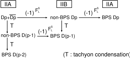
Figure 2.2: The descent relation

Moreover if we start with multiple non-BPS systems we can consider the decay of them to D-branes with lower codimensions more than two. This can be stated as

$$2^{m-1}~{}\mbox{pairs of}~{}Dp+\overline{Dp}~{} \rightarrow ~{}\left\{\begin{array}[]{l}\mbox{one non-BPS}~{}D(p-2m+1)\mbox{-brane},\\ \mbox{one BPS}~{}D(p-2m)\mbox{-brane},\end{array}\right.$$ (2.4.79)

$$2^{m-1}~{}\mbox{Non-BPS}~{}Dp\mbox{-brane} \rightarrow ~{}\mbox{one BPS}~{}D(p-2m+1)\mbox{-brane}.$$ (2.4.80)

The reason why we have to prepare $2^{m-1}$ pairs is related to K-theory, which is a mathematical theory as an extension of cohomology [11, 12]. In this thesis we do not explain it.

Now the problem is how we can understand these decay channels. The easiest and the most intuitive way is to consider the field theory on these D-branes. In general it is known that the Yang-Mills theory exists on BPS D-branes because of the massless gauge field $A_{\mu}(x)$ on them. As we saw in the last subsection the massless gauge fields also exist in both brane-antibranes and non-BPS D-branes, therefore we expect that some kind of gauge theory exists on these D-brane systems, too. Indeed this expectation turns out to be correct and it is known that those field theories can be roughly approximated by scalar-QED or Yang-Mills-Higgs theories [59].

As an example let us consider the decay of a non-BPS D9-brane and the field theory on it. For simplicity we ignore massive fields and all fermionic fields on these D-brane systems and we pay attention to the massless gauge field $A_{\mu}(x)$ and the tachyon field $T(x)$. The most important thing here is that the tachyon field is a scalar field, thus it has a scalar potential, which is called tachyon potential. In figure 2.3 we have drawn a typical form of tachyon potential. There are two kinds of extremum points $T=0$ and $T=T_{0}$. The former is the maximum point where the non-BPS D9-brane exists, while at the latter point there are no D-branes and it represents the vacuum with only closed strings. The first decay channel of a non-BPS D9-brane corresponds to rolling down the tachyon potential from the top to the bottom, and the tachyon field $T(x)$ obtains the expectation value $T_{0}$.

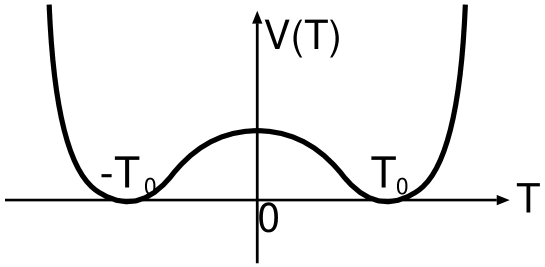
Figure 2.3: A typical shape of the tachyon potential

Now let us assume that the action for a non-BPS D9-brane is given by

$$S=\int d^{10}x\left(F^{\mu\nu}F_{\mu\nu}+\partial^{\mu}T\partial_{\mu}T+V(T)\right),$$ (2.4.81)

where $V(T)$ is the tachyon potential like figure 2.3. In this action we can consider a topologically nontrivial solution to the equation of motion of the tachyon field $T(x)$. The profile of the tachyon can be given by

$$T(x)\rightarrow\left\{\begin{array}[]{ll}T_{0}{}{}&(\mbox{at}~{}x^{1}\rightarrow\infty),\\ -T_{0}{}{}&(\mbox{at}~{}x^{1}\rightarrow-\infty).\end{array}\right.$$ (2.4.82)

This type of configuration is called a kink (see figure 2.4). From fig. 2.4 we can see that the tachyon field deletes the energy density of a non-BPS D9-brane almost everywhere except around $x^{1}=0$. Therefore we can guess that a codimension one D-brane remains at $x^{1}=0$ after the decay of a non-BPS D9-brane. This is just a BPS D8-brane, and this process corresponds to the second decay channel of non-BPS D9-branes.

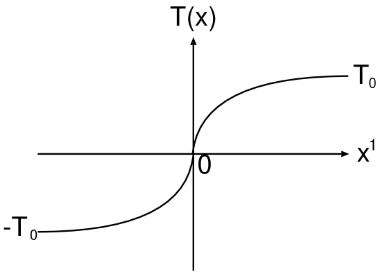
Figure 2.4: The kink profile of the tachyon $T(x)$

In both decay channels the tachyon field obtains the expectation value and this kind of process is called tachyon condensation. However, the conjecture of decay of D-branes can not exactly be verified by using the conventional field theory action like eq.(2.4.81). Indeed, this action can not explain the fact that at $T=T_{0}$ there does not remain any matter from open strings because of the absence of any D-branes. According to the conjecture, the action $S$ should be equal to zero at $T=T_{0}$, while in the conventional field theory the kinetic term $F^{\mu\nu}F_{\mu\nu}+\partial^{\mu}T\partial_{\mu}T$ remains.

To verify these correctly we have to proceed to a more extended field theory for strings, which includes $\alpha^{\prime}$ corrections. It is called string field theory. Indeed the action of string field theory includes the infinite number of derivatives, and it is nonlocal. The nonlocality of that action explains the complete vanishing of the matter at the minimum point of tachyon potential. In the next chapter we will verify the conjecture of tachyon condensation by using string field theory.

2.5 Are Non-BPS Systems Physical?

Now we have explained all kinds of unstable D$p$-brane systems in Type II theories, while the situation in Type I theory, which we do not deal with in this thesis, is a little more complicated.

In Type I theory there appear several stable non-BPS D$p$-branes. The reason why they become stable comes from the fact that the orientifold projection $\frac{1+\Omega}{2}$ in the open string partition function projects out the tachyon field. It is known that the stable non-BPS D0-brane plays an important role in the discussion about the Type I and Heterotic duality [60]. According to the prediction of string duality between Type I and Heterotic theory, there should exist an object in the Heterotic theory which corresponds to the non-BPS D0-brane in Type I theory. The duality between these two theories is known to be a strong-weak duality (S-duality), thus we can predict that the corresponding object in the Heterotic theory is not a solitonic object but a fundamental object because the non-BPS D-brane is a solitonic object in Type I theory. In fact, the author in [39] showed that the non-BPS D0-brane (non-BPS D-particle) in Type I theory corresponds to the firstly-excited massive state of a fundamental closed string in the Heterotic theory, by the discussion about the comparison of quantum numbers between them.

Since then, there have appeared other similar arguments about non-BPS systems by using string dualities like Type II/$K3$ and Hetero$/T^{4}$ duality [44]. In this way we started to recognize that the non-BPS D-branes (and also other non-BPS systems) are important physical objects in string theory.

Chapter 3 Off-Shell Description of Tachyon Condensation

In the previous chapter we have introduced the non-BPS D-brane systems in string theory and have explained the decay of those D-branes called tachyon condensation. In this chapter we would like to prove that conjecture in the quantitative way. The best and natural way to describe the tachyon condensation is to use string field theory. Especially since we deal with the decay of D-branes, we need open string field theory. In this theory we usually choose and fix the closed string background and we can obtain the “stringy” type of field theory picture of open strings like the tachyon potential which was explained in section 2.4.

Now several kinds of formulations of open string field theory are known. The most famous one is Witten’s cubic string field theory [15, 16] or its nonpolynomial extension by Berkovits [17]. Of course, these string field theories have given good support [18, 19, 20] to the conjecture by calculating the tachyon potential, although its analysis called the level truncation method is approximate one. On the other hand, one of string field theories called boundary string field theory (BSFT) [22, 23, 24, 61, 62] is appropriate to describe the tachyon condensation exactly [22, 25, 26, 27, 28, 29]. In this chapter we will introduce the formulation of boundary string field theory, and by using it we will calculate the action of string field theory and the tachyon potential. In addition we will prove the conjecture about the tachyon condensation.

3.1 The Relation between the Worldsheet RG Flow and the Tachyon Condensation

In this and next sections we will introduce the formalism of boundary string field theory (BSFT). Here we will discuss it in both of the bosonic string [22, 23, 24] and the superstring [61, 62] in the parallel way because there is not much formal difference between two.

BSFT is one type of string field theories which is defined on the total boundary space of the two dimensional sigma model. We start with the two dimensional sigma model action $I_{0}$ with the one dimensional boundary action $I_{B}$ on the disk. $I_{0}$ is defined inside the disk as the bulk action whose general form is written in the following way:

$$I_{0} = \frac{1}{4\pi}\int d^{2}zd^{2}\theta[G_{\mu\nu}({\bf X})+B_{\mu\nu}({\bf X})]D_{\bar{\theta}}{\bf X}^{\nu}D_{\theta}{\bf X}^{\mu}$$ (3.1.1)

$$= \frac{1}{4\pi}\int d^{2}z\Bigl{\{}[G_{\mu\nu}(X)+B_{\mu\nu}(X)]\partial X^{\mu}\bar{\partial}X^{\nu}$$

$$~{}~{}~{}~{}~{}~{}~{}~{}~{}~{}~{}+G_{\mu\nu}(X)(-i\psi^{\mu}_{L}\bar{{\cal D}}\psi^{\nu}_{L}+i\psi^{\mu}_{R}{\cal D}\psi^{\nu}_{R})+\frac{1}{2}R_{\mu\nu\rho\sigma}(X)\psi^{\mu}_{L}\psi^{\nu}_{L}\psi^{\rho}_{R}\psi^{\sigma}_{R}\Bigr{\}},$$

where

$$D_{\theta} = \partial_{\theta}+\theta\partial~{}~{},~{}~{}D_{\bar{\theta}}=\partial_{\bar{\theta}}+\bar{\theta}\bar{\partial},$$

$${\bf X}^{\mu} = X^{\mu}+i^{\frac{1}{2}}\theta\psi^{\mu}_{L}-i^{-\frac{1}{2}}\bar{\theta}\psi^{\mu}_{R}+\theta\bar{\theta}F^{\mu},$$

$$\bar{{\cal D}}\psi^{\nu}_{L} = \bar{\partial}\psi^{\nu}_{L}+\left[\Gamma^{\nu}_{\rho\sigma}(X)+\frac{1}{2}H^{\nu}_{~{}\rho\sigma}(X)\right]\bar{\partial}X^{\rho}\psi_{L}^{\sigma},$$

$${\cal D}\psi^{\nu}_{R} = \partial\psi^{\nu}_{R}+\left[\Gamma^{\nu}_{\rho\sigma}(X)-\frac{1}{2}H^{\nu}_{~{}\rho\sigma}(X)\right]\partial X^{\rho}\psi_{R}^{\sigma},$$

$F^{\mu}$ is an auxiliary field in the worldsheet and $H^{\nu}_{~{}\rho\sigma}(X)$ is the field strength of NSNS B-field $B_{\mu\nu}(X)$. Here we have omitted all terms with ghosts $(b,c~{};~{}\beta,\gamma)$. If we want to consider the bosonic string theory we have only to remove the terms including worldsheet fermions $(\psi^{\mu}_{L},~{}\psi^{\mu}_{R})$ and superconformal ghosts $(\beta,~{}\gamma)$ from the above action.

On the other hand, the action $I_{B}$ is defined on the boundary of disk. This boundary part is the most important part in BSFT and it consists of all kinds of fields on the boundary of disk. For example, the most general form of boundary action $I_{B}$ for the bosonic string theory can be written by

$$I_{B}=\int^{\pi}_{-\pi}\frac{d\tau}{2\pi}~{}{\cal V}(X^{\mu}(\tau),b(\tau),c(\tau)),$$ (3.1.3)

where

$${\cal V}(X^{\mu},b,c) = T(X)+\dot{X}^{\mu}A_{\mu}(X)+\dot{X}^{\mu}\dot{X}^{\nu}C_{\mu\nu}(X)+\ddot{X}^{\mu}D_{\mu}(X)+\cdots\cdots$$ (3.1.4)

$$\equiv \sum_{i}\lambda^{i}{\cal V}_{i}(X^{\mu},b,c).$$

Here in the first line of eq.(3.1.4) we have omitted terms with $b,~{}c$ ghosts, and $\lambda^{i}$ are coupling constants in the two dimensional sigma model, which represent various target space fields. For example if we expand the first term of eq.(3.1.4) like

$$T(X)=a_{0}+a_{1\mu}X^{\mu}+a_{2\mu\nu}X^{\mu}X^{\nu}+\cdots\cdots,$$ (3.1.5)

various coefficients $a_{0},a_{1\mu},a_{2\mu\nu},\cdots$ are a part of coupling constants $\lambda^{i}$. The boundary action (3.1.4) is for the bosonic string, while there are some subtle points to write down the explicit form of boundary action for the superstring as we will see later in section 3.3. For this reason we will explain only the summary of the idea of BSFT by using the action (3.1.4). The idea is completely the same as that of the superstring.

In the action (3.1.4) $T(X)$ represents an open string tachyon, $A_{\mu}(X)$ a gauge field and the other fields like $C_{\mu\nu}(X)$ and $D_{\mu}(X)$ massive modes of open strings on a bosonic D-brane. In the language of statistical mechanics the tachyon field has a dimension less than 1, which corresponds to a relevant operator, the gauge field has dimension 1 (marginal), and the other fields have dimensions greater than 1 (irrelevant). This fact means that we have included all operators which break the conformal invariance. Note that we have broken the conformal invariance only on the boundary of disk and not inside the disk. This means that we fix a closed string background to satisfy the equation of motion of (super)gravity (“on-shell”), while we do not require the equation of motion of (super)Maxwell theory (“off-shell”). In general the off-shell string theory is described by (open) string field theory. Therefore, to consider the sigma model action like eq.(3.1.4) is one of descriptions of extending an on-shell theory to an off-shell one, and boundary string field theory (BSFT) is based on this idea. Here, the name “boundary” comes from the boundary perturbation in action (3.1.4). Moreover, another feature of this theory is that we can see the explicit background independence of closed strings in action (3.1.1). For this reason, the original name of this formalism in the paper [22] was “background independent open string field theory”.

Before the construction of BSFT, we will explain the relation between the renormalization group of the sigma model and the physical picture of decay of D-branes. When we consider the general nonlinear sigma model which breaks the conformal invariance like eq.(3.1.4), the renormalization group flow starts and the theory flows out of a conformal fixed point and leaves for another fixed point. Especially relevant operators play the most important role to cause the renormalization group flow, and these relevant operators are tachyons which can be seen in eq.(3.1.4). Therefore, in the language of the target space of string theory, we can identify the renormalization group flow as the process of tachyon condensation, which means that the tachyon fields have their expectation values. In string theory (open string) tachyon fields appear when a D-brane is perturbatively unstable, thus we can also say that the renormalization group flow represents the decay process of the D-brane. The UV fixed point where the renormalization group starts corresponds to the situation that there is an unstable D-brane in the target space. When that flow reaches the final IR fixed point, the D-brane completely decays and a stable vacuum or a stable D-brane appears. However, to discuss the decay of D-branes in the quantitative way we need some physical quantity. That is just the target space action $S$ (action of string field theory) for fields $T(x),~{}A_{\mu}(x),~{}\cdots$ in eq.(3.1.4) or tachyon potential $V(T)$, which is derived from $S$. Indeed there is a relation between the tachyon potential and the renormalization group flow [52], and it is drawn in figure 3.1.

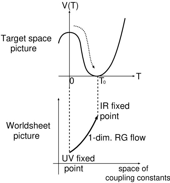
Figure 3.1: The relation between one-dimensional renormalization group flow and the tachyon potential. On top of the potential unstable D-branes live. After its tachyon condensation those D-branes disappear at the bottom of the potential.

In figure 3.1 the conformal invariance is kept only at the extremum points $T=0$ and $T=T_{0}$. In the conventional first-quantized string theory we fix the open string background at either $T=0$ or $T=T_{0}$ and usually investigate the scatterings (S-matrices) of the fluctuating fields around $T=0$ or $T=T_{0}$. Therefore from the first-quantized string theory we can not see how two vacuums $T=0$ and $T=T_{0}$ are related or connected with each other. Its relation can not be understood without the tachyon potential. In this chapter we will explain that BSFT determines the action of string field theory and the tachyon potential.

3.2 The Batalin-Vilkovisky Formulation of Boundary String Field Theory

In this section we will introduce the Batalin-Vilkovisky(BV) formalism [63] because the construction of BSFT is based on it [22]. The BV formalism has been used in order to construct various string field theories like cubic open string field theory and closed string field theories.

First we start with a supermanifold $M$ equipped with U(1) symmetry that we will call the ghost number. The essential element in the BV formalism is the symplectic structure and we can define a fermionic non-degenerate two-form $\omega$ with U(1) charge $-1$ which is closed, $d\omega=0$ . If we define the local coordinate $\lambda^{i}~{}(i=1,2,\cdots,\mbox{dim}M)$ to express the manifold, then we can consider the Poisson bracket given by

$$\{F,G\}=\frac{\partial_{r}F}{\partial\lambda^{i}}\omega^{ij}\frac{\partial_{l}G}{\partial\lambda^{j}},$$ (3.2.6)

where $\omega^{ij}$ is the inverse matrix of $\omega_{ij}$, and $\frac{\partial_{r}}{\partial\lambda^{i}},~{}\frac{\partial_{l}}{\partial\lambda^{j}}$ denote the right-derivative and the left-derivative respectively. By using these elements we can define the classical master equation for the action $S$ of string field theory as follows:

$$\{S,S\}=0.$$ (3.2.7)

This is the standard description of the BV formalism, while we can find a more convenient form of equation which is equivalent to eq.(3.2.7). To do it let us introduce a fermionic vector field $V=V^{i}\frac{\partial}{\partial\lambda^{i}}$ with U(1) charge $1$. If we consider the infinitesimal diffeomorphism $\lambda^{i}\rightarrow\lambda^{i}+\epsilon V^{i}$, the symplectic form $\omega$ transforms as $\omega\rightarrow\omega+\epsilon({\cal L}_{V}\omega)$, where ${\cal L}_{V}$ is the Lie derivative along the direction of the vector field $V$. It can also be defined by

$${\cal L}_{V}=di_{V}+i_{V}d,$$ (3.2.8)

where $i_{V}$ is the operation of contraction with $V$. If we assume that $V$ is a killing vector field, it generates a symmetry of $\omega$ and satisfies

$${\cal L}_{V}\omega=0.$$ (3.2.9)

From the definition of ${\cal L}_{V}$ in eq.(3.2.8) and the fact that $\omega$ is closed ($d\omega=0$), it can also be written as

$$d(i_{V}\omega)=0.$$ (3.2.10)

Here we claim that if the vector field $V$ is nilpotent ($V^{2}=0$) and satisfies the killing condition (${\cal L}_{V}\omega=0$), the following equation is equivalent to the master equation (3.2.7):

$$i_{V}\omega=dS.$$ (3.2.11)

The component form of this equation is given by

$$V^{j}\omega_{ji}=\frac{\partial_{l}S}{\partial\lambda^{i}}.$$ (3.2.12)

Note that the killing condition (3.2.10) guarantees that $S$ exists as a local solution to equation (3.2.11).

Let us prove the above statement. First we can easily check that the following identity holds

$${\cal L}_{V}i_{W}+i_{W}{\cal L}_{V}=i_{VW+WV},$$ (3.2.13)

where $V$ and $W$ are any fermionic vector fields. By setting $W=V$ and using the nilpotency of $V$ and the killing condition (3.2.9) we can obtain

$${\cal L}_{V}i_{V}\omega=0.$$ (3.2.14)

From the definition of ${\cal L}_{V}$ in eq.(3.2.8) and equation (3.2.10), the above equation becomes

$$di_{V}i_{V}\omega=d\left(V^{i}\frac{\partial_{l}S}{\partial\lambda^{i}}\right)=d\{S,S\}=0.$$ (3.2.15)

Here we have used equation (3.2.12). Thus, we can find that the nilpotency $V^{2}=0$ and the killing condition (3.2.9) lead equation (3.2.11) to $\{S,S\}=\mbox{constant}$. If we consider that this equation should also hold at on-shell regions ($dS=0$), the value of $\{S,S\}$ becomes equal to zero. This is the proof of the equivalence between the classical master equation (3.2.7) and eq.(3.2.11).

Now we are ready to apply this BV-formalism to the sigma model action for constructing BSFT. In BSFT we regard $\lambda^{i}$ and $S(\lambda)$ in eq.(3.2.12) as the target space fields and the action of string field theory, respectively. Thus, the supermanifold $M$ is the infinite dimensional space ($\mbox{dim}M=\infty$) spanned by all kinds of target space fields. The difficult thing here is to construct $V,\omega$ in eq.(3.2.11) by using the language of valuables in the two-dimensional sigma model. First we can identify the fermionic killing vector field $V$ as the bulk BRST operator $Q_{B}$ in the worldsheet since this operator satisfies the nilpotency condition and has U(1) charge $1$ if we define U(1) charge by the worldsheet ghost number. Next we express the closed two-form $\omega$ by using boundary fields in action (3.1.4) in the following way

$$\omega(\lambda) = \frac{1}{2}\omega_{ij}(\lambda)d\lambda^{i}\wedge d\lambda^{j},$$

$$\omega_{ij}(\lambda) = \left\{\begin{array}[]{ll}{\displaystyle\frac{1}{2}\int^{\pi}_{-\pi}\frac{d\tau_{1}}{2\pi}\int^{\pi}_{-\pi}\frac{d\tau_{2}}{2\pi}~{}\langle c{\cal V}_{i}(\tau_{1})c{\cal V}_{j}(\tau_{2})\rangle_{\lambda}{}{}}&(\mbox{bosonic string}),\\ &\\ {\displaystyle\frac{1}{2}\int^{\pi}_{-\pi}\frac{d\tau_{1}}{2\pi}\int^{\pi}_{-\pi}\frac{d\tau_{2}}{2\pi}~{}\langle ce^{-\phi}{\cal W}_{i}(\tau_{1})ce^{-\phi}{\cal W}_{j}(\tau_{2})\rangle_{\lambda}{}{}}&(\mbox{superstring}),\end{array}\right.$$ (3.2.19)

where $c(\tau)$ and $e^{-\phi}(\tau)$ are the ghost and the bosonized superconformal ghost, respectively. ${\cal V}_{i}(\tau_{1})$ and ${\cal V}_{j}(\tau_{2})$ are vertex operators of fields in the boundary action (3.1.4), while ${\cal W}_{i}(\tau_{1})$ and ${\cal W}_{j}(\tau_{2})$ are those with $-1$ picture. The correlator $\langle\cdots\rangle_{\lambda}$ is evaluated with a non-conformal boundary action like eq.(3.1.4), and in the path-integral formalism it is represented by

$$\langle\cdots\rangle_{\lambda}=\left\{\begin{array}[]{ll}{\displaystyle\int DX~{}\cdots~{}\exp[-I_{0}(X)-I_{B}(X)]{}{}}&(\mbox{bosonic string}),\\ &\\ {\displaystyle\int DXD\psi~{}\cdots~{}\exp[-I_{0}(X,\psi)-I_{B}(X,\psi)]{}{}}&(\mbox{superstring}).\end{array}\right.$$ (3.2.22)

where $\lambda^{i}$ is included in the boundary action $I_{B}$ like eq.(3.1.4). This definition of $\omega$ is quite desirable. Indeed it has the correct U(1) charge because the worldsheet ghost number of $\omega$ is $-1$. Moreover, it satisfies the necessary identities $d\omega={\cal L}_{V}\omega=0$ and the non-degeneracy (for proof, see [22, 62]).

Therefore we can rewrite equation (3.2.12) in terms of the boundary fields as follows

$$\frac{\partial S}{\partial\lambda^{i}}=\left\{\begin{array}[]{ll}{\displaystyle\frac{1}{2}\int^{\pi}_{-\pi}\frac{d\tau_{1}}{2\pi}\int^{\pi}_{-\pi}\frac{d\tau_{2}}{2\pi}~{}\langle c{\cal V}_{i}(\tau_{1})\{Q_{B},c{\cal V}(\tau_{2})\}\rangle_{\lambda}{}{}}&(\mbox{bosonic string}),\\ &\\ {\displaystyle\frac{1}{2}\int^{\pi}_{-\pi}\frac{d\tau_{1}}{2\pi}\int^{\pi}_{-\pi}\frac{d\tau_{2}}{2\pi}~{}\langle ce^{-\phi}{\cal W}_{i}(\tau_{1})\{Q_{B},ce^{-\phi}{\cal W}(\tau_{2})\}\rangle_{\lambda}{}{}}&(\mbox{superstring}),\end{array}\right.$$ (3.2.26)

where ${\cal V}=\lambda^{i}{\cal V}_{i}$ and ${\cal W}=\lambda^{i}{\cal W}_{i}$. Note that we have used the following relation

$$\left\{Q_{B},c{\cal V}(\tau_{2})\right\}=\left\{Q_{B}^{j}\frac{\partial}{\partial\lambda^{j}},\lambda^{k}c{\cal V}_{k}(\tau_{2})\right\}=Q_{B}^{j}\left(c{\cal V}_{j}(\tau_{2})\right).$$ (3.2.27)

The next step is to solve the above equation and to obtain the explicit form of action $S$. It is known that the solution to this equation can be obtained if we restrict possible boundary terms in action (3.1.3) to those which do not include the worldsheet ghosts $(b,~{}c)$ and superghosts $(\beta,~{}\gamma)$. In this case the action $S$ is given by

$$S(\lambda)=\left\{\begin{array}[]{cl}{\displaystyle\left(\beta^{i}(\lambda)\frac{\partial}{\partial\lambda^{i}}+1\right)Z(\lambda){}{}}&(\mbox{bosonic string}),\\ &\\ {\displaystyle Z(\lambda){}{}}&(\mbox{superstring}),\end{array}\right.$$ (3.2.31)

where $\beta^{i}(\lambda)$ is the beta function of the coupling constant $\lambda^{i}$ and $Z(\lambda)$ is the partition function of the matter part on the disk, which is given by

$$Z(\lambda)=\left\{\begin{array}[]{ll}{\displaystyle\int DX~{}\exp[-I_{0}(X)-I_{B}(X)]{}{}}&(\mbox{bosonic string}),\\ &\\ {\displaystyle\int DXD\psi~{}\exp[-I_{0}(X,\psi)-I_{B}(X,\psi)]{}{}}&(\mbox{superstring}).\end{array}\right.$$ (3.2.33)

The important point is that $I_{B}$ is a non-conformal boundary action like eq.(3.1.3) which does not include the worldsheet ghosts $(b,~{}c)$ and superghosts $(\beta,~{}\gamma)$.

Now let us prove this relation. First we can easily calculate the anticommutators in eq.(3.2.26) and its result is

$$\{Q_{B},c{\cal V}_{i}(\tau_{2})\} = (1-\Delta_{i})c\dot{c}{\cal V}_{i}(\tau_{2}),$$

$$\{Q_{B},c{\cal W}_{i}(\tau_{2})\} = \left(\frac{1}{2}-\Delta_{i}\right)c\dot{c}{\cal W}_{i}(\tau_{2}),$$ (3.2.34)

where $\Delta_{i}$ is the conformal dimension of the primary operator ${\cal V}_{i}(\tau)$ or ${\cal W}_{i}(\tau)$. From this we can obtain the following expression

$$\frac{\partial S}{\partial\lambda^{i}}=\left\{\begin{array}[]{ll}{\displaystyle-(1-\Delta_{j})\lambda^{j}G_{ij}(\lambda){}{}}&(\mbox{bosonic string}),\\ &\\ {\displaystyle-\left(\frac{1}{2}-\Delta_{j}\right)\lambda^{j}G_{ij}(\lambda){}{}}&(\mbox{superstring}),\end{array}\right.$$ (3.2.38)

where

$$G_{ij}(\lambda)=\left\{\begin{array}[]{ll}{\displaystyle 2\int^{\pi}_{-\pi}\frac{d\tau_{1}}{2\pi}\int^{\pi}_{-\pi}\frac{d\tau_{2}}{2\pi}\sin^{2}\left(\frac{\tau_{1}-\tau_{2}}{2}\right)\langle{\cal V}_{i}(\tau_{1}){\cal V}_{j}(\tau_{2})\rangle_{\lambda}{}{}}&(\mbox{bosonic string}),\\ &\\ {\displaystyle\int^{\pi}_{-\pi}\frac{d\tau_{1}}{2\pi}\int^{\pi}_{-\pi}\frac{d\tau_{2}}{2\pi}\sin\left(\frac{\tau_{1}-\tau_{2}}{2}\right)\langle{\cal W}_{i}(\tau_{1}){\cal W}_{j}(\tau_{2})\rangle_{\lambda}{}{}}&(\mbox{superstring}).\end{array}\right.$$ (3.2.42)

Here we have used a three-point correlation function of ghosts and a two-point one of superconformal ghosts

$$\langle c(\tau_{1})c\dot{c}(\tau_{2})\rangle = -4\sin^{2}\left(\frac{\tau_{1}-\tau_{2}}{2}\right),$$

$$\langle e^{-\phi}(\tau_{1})e^{-\phi}(\tau_{2})\rangle = \frac{1}{2}\sin^{-1}\left(\frac{\tau_{1}-\tau_{2}}{2}\right).$$ (3.2.43)

The ghost part and superconformal ghost part appear only in the above correlation functions because we have imposed the assumption that the boundary action $I_{B}$ and the vertex operators ${\cal V}_{i}(\tau),~{}{\cal W}_{i}(\tau)$ do not include any terms with $b,c,\beta$ and $\gamma$. Therefore the later calculation depends only on the matter part.

Here we will use a trick to prove eq.(3.2.31) in the formal way. First we start with the case of the bosonic string theory. We assume that the matter vertex operators in eq.(3.1.4) consist of two kinds of operators which are completely decoupled from each other. We denote one by ${\cal V}_{1i}$ and the other by ${\cal V}_{2i}$, and the vertex operator ${\cal V}$ is written as

$${\cal V}=\sum_{i}\lambda_{1}^{i}{\cal V}_{1i}+\sum_{j}\lambda_{2}^{j}{\cal V}_{2j}.$$ (3.2.44)

Inserting this into eq.(3.2.42) we can see that there appear three kinds of two point functions : $\langle{\cal V}_{1i}(\tau_{1}){\cal V}_{1j}(\tau_{2})\rangle_{\lambda},~{}\langle{\cal V}_{2i}(\tau_{1}){\cal V}_{2j}(\tau_{2})\rangle_{\lambda}$ and $\langle{\cal V}_{1i}(\tau_{1}){\cal V}_{2j}(\tau_{2})\rangle_{\lambda}$. The third type of two-point functions splits into products of one-point functions $\langle{\cal V}_{1i}(0)\rangle_{\lambda_{1}}\times\langle{\cal V}_{2j}(0)\rangle_{\lambda_{2}}$, where the dependence of $\tau$ is dropped because of the rotational invariance of $\tau$ on the boundary of disk. If we use an identity of a simple integral

$$2\int^{\pi}_{-\pi}\frac{d\tau_{1}}{2\pi}\int^{\pi}_{-\pi}\frac{d\tau_{2}}{2\pi}\sin^{2}\left(\frac{\tau_{1}-\tau_{2}}{2}\right)=1,$$ (3.2.45)

we can obtain the following expression of $dS\left(=\sum_{i}d\lambda^{i}\frac{\partial S}{\partial\lambda^{i}}\right)$:

$$dS = \left(a_{2}^{j}\frac{\partial Z_{2}}{\partial\lambda^{j}_{2}}(\lambda_{2})\right)dZ_{1}(\lambda_{1})+\left(a_{1}^{j}\frac{\partial Z_{1}}{\partial\lambda^{j}_{1}}(\lambda_{1})\right)dZ_{2}(\lambda_{2})$$ (3.2.46)

$$~{}~{}~{}~{}~{}~{}~{}~{}~{}~{}+Z_{2}(\lambda_{2})\left(d\lambda^{i}_{1}V_{1i}(\lambda_{1})\right)+Z_{1}(\lambda_{1})\left(d\lambda^{i}_{2}V_{2i}(\lambda_{2})\right),$$

where

$$a_{1}^{j}(\lambda_{1}) = -(1-\Delta_{1j})\lambda^{j}_{1},$$

$$a_{2}^{j}(\lambda_{2}) = -(1-\Delta_{2j})\lambda^{j}_{2},$$

$$V_{1i}(\lambda_{1}) = -(1-\Delta_{1j})\lambda^{j}_{1}G_{ij}(\lambda_{1}),$$

$$V_{2i}(\lambda_{2}) = -(1-\Delta_{2j})\lambda^{j}_{2}G_{ij}(\lambda_{2}).$$ (3.2.47)

Here $Z_{1}(\lambda_{1})~{}\left(\mbox{or}~{}Z_{2}(\lambda_{2})\right)$ is the disk partition function whose boundary action $I_{B}$ is given by $\sum_{i}\lambda_{1}^{i}{\cal V}_{1i}~{}\left(\mbox{or}~{}\sum_{j}\lambda_{2}^{j}{\cal V}_{2j}\right)$. $dZ_{1}(\lambda_{1})~{}\left(\mbox{or}~{}dZ_{2}(\lambda_{2})\right)$ is defined by $\sum_{i}d\lambda_{1}^{i}\frac{\partial Z_{1}}{\partial\lambda_{1}^{i}}~{}\left(\mbox{or}~{}\sum_{j}d\lambda_{2}^{j}\frac{\partial Z_{2}}{\partial\lambda_{2}^{j}}\right)$, and $\frac{\partial Z_{1}}{\partial\lambda_{1}^{i}}~{}\left(\mbox{or}~{}\frac{\partial Z_{2}}{\partial\lambda_{2}^{j}}\right)$ is equal to the one-point function $\langle{\cal V}_{1i}\rangle_{\lambda_{1}}~{}\left(\mbox{or}~{}\langle{\cal V}_{2j}\rangle_{\lambda_{2}}\right)$. Since we have assumed that the matter sector is split into two parts which are completely decoupled from each other, we can easily see that the total disk partition function $Z(\lambda)$ is equal to $Z_{1}(\lambda_{1})Z_{2}(\lambda_{2})$.

Next, due to $ddS=0$ the right-hand side of eq.(3.2.46) obeys some constraint equation. Especially the term including $d\lambda_{1}^{i}\wedge d\lambda_{2}^{j}$ should be

$$0 = dZ_{1}(\lambda_{1})\wedge\left\{d\lambda^{i}_{2}V_{2i}(\lambda_{2})-d\left(a_{2}^{j}\frac{\partial Z_{2}}{\partial\lambda^{j}_{2}}(\lambda_{2})\right)\right\}$$ (3.2.48)

$$+\left\{d\left(a_{1}^{j}\frac{\partial Z_{1}}{\partial\lambda^{j}_{1}}(\lambda_{1})\right)-d\lambda^{i}_{1}V_{1i}(\lambda_{1})\right\}\wedge dZ_{2}(\lambda_{2}).$$

This equation implies that we can divide this equation into two parts which depend only on either $\lambda_{1}$ or $\lambda_{2}$ and we can obtain the following equations:

$$d\left(a_{1}^{j}\frac{\partial Z_{1}}{\partial\lambda^{j}_{1}}(\lambda_{1})\right)-d\lambda^{i}_{1}V_{1i}(\lambda_{1}) = -kdZ_{1}(\lambda_{1}),$$

$$d\lambda^{i}_{2}V_{2i}(\lambda_{2})-d\left(a_{2}^{j}\frac{\partial Z_{2}}{\partial\lambda^{j}_{2}}(\lambda_{2})\right) = kdZ_{2}(\lambda_{2}),$$ (3.2.49)

where $k$ is some constant. By using these equations and erasing $V_{1i}$ and $V_{2i}$, equation (3.2.46) becomes

$$dS=d\left\{\left(a^{i}_{1}(\lambda_{1})\frac{\partial}{\partial\lambda_{1}^{i}}+a^{i}_{2}(\lambda_{2})\frac{\partial}{\partial\lambda_{2}^{i}}+k\right)Z_{1}(\lambda_{1})Z_{2}(\lambda_{2})\right\},$$ (3.2.50)

and up to a constant the string field action $S$ is determined as

$$S=\left(a^{i}_{1}(\lambda_{1})\frac{\partial}{\partial\lambda_{1}^{i}}+a^{i}_{2}(\lambda_{2})\frac{\partial}{\partial\lambda_{2}^{i}}+k\right)Z_{1}(\lambda_{1})Z_{2}(\lambda_{2}).$$ (3.2.51)

Until now we have assumed that the matter system consists of two parts which are decoupled from each other, while the above result can naturally be extended to the general one as

$$S(\lambda)=\left(a^{i}(\lambda)\frac{\partial}{\partial\lambda^{i}}+k\right)Z(\lambda),$$ (3.2.52)

where

$$a^{i}(\lambda)=-(1-\Delta_{i})\lambda^{i}.$$ (3.2.53)

Here the parameter $k$ is related to overall normalization of the partition function $Z$ which depends on the convention, and it can not be determined from eq.(3.2.42). Thus, we fix it by hand to $k=1$.

By the way, the result (3.2.52) does not look covariant under the reparametrization of $\lambda$ like $\lambda^{i}\rightarrow f^{i}(\lambda)$. To solve this issue let us recall that the general form of beta function of $\lambda^{i}$ is given by

$$\beta^{i}(\lambda)=-(1-\Delta_{i})\lambda^{i}+O(\lambda^{2}).$$ (3.2.54)

Next notice that in the renormalization group theory the beta function $\beta^{i}(\lambda)$ can be set to the linear function of $\lambda^{i}$ if we take the appropriate redefinition of $\lambda^{i}$. Therefore we can also write equation (3.2.52) as

$$S(\lambda)=\left(\beta^{i}(\lambda)\frac{\partial}{\partial\lambda^{i}}+1\right)Z(\lambda).$$ (3.2.55)

In the same way we can replace eq.(3.2.38) with:

$$\frac{\partial S}{\partial\lambda^{i}}=\beta^{j}(\lambda)G_{ij}(\lambda).$$ (3.2.56)

This is the covariant form, and we have found that BSFT chooses the special coordinate of $\lambda^{i}$ so that their beta functions become linear.

Now we have completed the proof of eq.(3.2.31) in the case of bosonic string. This method of proof is also available in the case of superstring if we replace ${\cal V}_{i}$ by ${\cal W}_{i}$. The only difference is that one point function $\langle{\cal W}_{i}(0)\rangle_{\lambda}$ becomes zero because ${\cal W}_{i}$ is a vertex operator with $(-1)$ picture and its worldsheet statistics is fermionic. Thus, the first two terms in eq.(3.2.46) become zero, and as a result the term with the derivative of $\lambda^{i}$ in eq.(3.2.55) vanishes. Therefore, the action of superstring field theory becomes equal to just the partition function like eq.(3.2.31). Moreover, the same relation as eq.(3.2.56) holds if we notice that in the superstring the beta function of $\lambda^{i}$ is given by

$$\beta^{i}(\lambda)=-\left(\frac{1}{2}-\Delta_{i}\right)\lambda^{i}+O^{2}(\lambda).$$ (3.2.57)

By the way, from eq.(3.2.31) we can claim that the action $S(\lambda)$ is an off-shell (non-conformal) generalization of the boundary entropy $g$ [64]. The boundary entropy is defined in the statistical mechanics as the internal product of the boundary state and the conformal vacuum, and it is just equal to the disk partition function:

$$g=\langle 0|B\rangle=Z_{disk}(\Sigma_{B}),$$ (3.2.58)

where $|B\rangle$ can be any boundary state like eq.(2.2.54), and the proof of equivalence of $\langle 0|B\rangle$ and $Z_{disk}(\Sigma_{B})$ is shown in appendix B. Moreover, if we use the explicit form of boundary state, we can find out that the boundary entropy is equal to the mass of the D-brane. This is the physical meaning of the boundary entropy in on-shell string theory, and we can regard the action $S$ as an off-shell (non-conformal) generalization of the boundary entropy. This is obvious in the superstring because $S$ is completely equal to the partition function even in the off-shell region like eq.(3.2.31), while we can also find out that this statement is meaningful even in the bosonic string too.

One property supporting the above statement is that it is equal to the disk partition function at on-shell (conformal) points

$$S(\lambda^{*})=Z(\lambda^{*}),$$ (3.2.59)

where $\lambda^{*}$ is a solution to $\beta^{i}(\lambda)=0$, which is the equation of motion of target space fields. The second is that the action $S$ of string field theory satisfies the famous g-theorem [64]. The g-theorem is the boundary analog of the c-theorem, which appears in the bulk conformal field theory, and there are two statements. The first statement is that the boundary entropy at the UV fixed point is always greater than at the IR fixed point:

$$g_{UV}>g_{IR}.$$ (3.2.60)

This means that the mass of an unstable D-brane is greater than that of a D-brane which appears after the decay of the unstable D-brane. This is a physically desirable result.

The second statement of the g-theorem is that the boundary entropy $g$ at the UV conformal fixed point monotonically decreases along the renormalization group flow and it takes the minimal value at the IR fixed point. In fact, we can show that the action $S$ of string field theory satisfies this statement. This is because the dependence of the action $S$ on the worldsheet cut-off scale $x$ is determined in the following way:

$$\frac{dS}{d\log|x|}=-\beta^{i}(\lambda)\frac{\partial}{\partial\lambda^{i}}S=-\beta^{i}\beta^{j}G_{ij}(\lambda),$$ (3.2.61)

where we have used equation (3.2.56) and the renormalization group equation:

$$\frac{d\lambda^{i}}{d\log|x|}=-\beta^{i}(\lambda).$$ (3.2.62)

If we notice that $G_{ij}(\lambda)$ is positive definite from the explicit form of it in eq.(3.2.42), we can see that the action $S$ monotonically decreases along the renormalization group flow. This is the proof of the second statement of the g-theorem.

From these facts we have found out that $S$ is equal to the mass of the unstable D-brane which decays and it also seems to be the same as the potential energy of the system. Therefore by investigating the action $S$ of string field theory we can verify the decay of unstable D-brane systems in the quantitative way. Moreover, these features of the action $S$ completely coincide with the content of section 3.1 and figure 3.1.

3.3 The Worldsheet Actions for Non-BPS Systems in the Superstring Theory

In the last section we have constructed the general framework of BSFT, and in section 3.1 we have explained its idea by using the boundary action $I_{B}$ (3.1.4) for the bosonic string. The reason why we have not written down the boundary action $I_{B}$ for the superstring theory is that its form is a little complicated and it also depends on which non-BPS system we would like to consider. In this section we will give the explicit form of boundary actions for the non-BPS D-brane and the brane-antibrane system in the superstring theory, and in section 3.5 we will concretely calculate the actions $S$ of string field theory for these systems by using the relation (3.2.31).

The two-dimensional bulk action is common in both of these systems and is given by eq.(3.1.1). This action is written by the two-dimensional superfield ${\bf X}^{\mu}$, thus it is natural to require the one-dimensional worldsheet supersymmetry in the boundary action $I_{B}$. The superspace representation in the one-dimensional theory is defined by:

$$\left\{\begin{array}[]{lcl}{\bf X}^{\mu}&=&X^{\mu}+2i\theta\psi^{\mu},\\ D_{\theta}&=&\frac{\partial}{\partial\theta}+\theta\frac{\partial}{\partial\tau}.\end{array}\right.$$ (3.3.65)

If we assign the worldsheet dimensions $0,1$ to $X^{\mu},~{}D_{\theta}$ and write all possible terms in the boundary action $I_{B}$ by using them, then it becomes as follows:

$$\int_{\partial\Sigma}d\tau d\theta\left[-iD_{\theta}{\bf X}^{\mu}A_{\mu}({\bf X})+\cdots\cdots\right],$$ (3.3.66)

where the field $A_{\mu}({\bf X})$ represents the gauge field and the terms $\cdots$ do all massive fields. Unfortunately in RNS formalism we can not include target space fermions such a gaugino in the sigma model action. This might be resolved by considering BSFT formalism in the Green-Schwarz formalism [65] or Berkovits’ pure spinor formalism [66]. We do not consider this problem here and will discuss it in the final chapter.

The more serious problem here is that in the above sigma model action we can not see any tachyonic fields. Indeed boundary action (3.3.66) is for a BPS D-brane. This means that if we write a one-dimensional supersymmetric action by using only the superfield ${\bf X}^{\mu}$, we can not include any relevant terms which represent tachyonic modes. To describe tachyon condensation on non-BPS systems we have to include relevant terms in the action.

3.3.1 For a brane-antibrane system

First we will consider the boundary action for a brane-antibrane system according to the description in subsection 2.3.3. In that subsection we have required the GSO-projection $(-1)^{F_{tot}}\equiv(-1)^{F}\times(-1)^{F_{CP}}=1$, where $F_{CP}$ gives the fermion number to the Chan-Paton factors, and assigns $\{+,-,-,+\}$ to $\{1,\sigma_{1},\sigma_{2},\sigma_{3}\}$. However, these Pauli matrices are not fermionic quantities but bosonic ones, and this statement is not precise. To describe this situation exactly we have to prepare some fermionic quantities which play the role similar to the Chan-Paton factors. To do this we should include some fermionic variable in the boundary worldsheet action $I_{B}$ instead of including the Chan-Paton degrees of freedom. Indeed in the next subsection we can see that this fermionic variable plays the same role as the Chan-Paton factors and obeys the GSO-projection which is described in subsection 2.3.3.

Now let us consider a complex fermionic superfield ${\bf\Gamma},~{}{\bf\bar{\Gamma}}$ defined by [28, 29, 11]

$${\bf\Gamma}=\eta+\theta F.$$ (3.3.67)

If we write the most general one-dimensional action by using ${\bf X}^{\mu},~{}{\bf\Gamma},~{}{\bf\bar{\Gamma}}$ and $D_{\theta}$ with their dimension $0,0,0,1$ respectively, then we can obtain the following action

$$I_{B} = \int_{\partial\Sigma}d\tau d\theta\Biggl{[}\frac{1}{\sqrt{2\pi}}{\bf\bar{\Gamma}}T({\bf X})+\frac{1}{\sqrt{2\pi}}\bar{T}({\bf X}){\bf\Gamma}$$ (3.3.68)

$$~{}~{}~{}~{}~{}~{}~{}~{}~{}~{}~{}~{}-{\bf\bar{\Gamma}}D_{\theta}{\bf\Gamma}-\frac{i}{2}D_{\theta}{\bf X}^{\mu}A^{(+)}_{\mu}({\bf X})+iA^{(-)}_{\mu}({\bf X})D_{\theta}{\bf X}^{\mu}{\bf\bar{\Gamma}}{\bf\Gamma}$$

$$~{}~{}~{}~{}~{}~{}~{}~{}~{}~{}~{}~{}~{}~{}~{}~{}~{}~{}+\cdots\cdots\Biggr{]},$$

where in each line of the above action relevant, marginal and irrelevant terms are shown. Here notice that several functionals $A^{\pm}_{\mu}({\bf X}),~{}T({\bf X})$ and $\bar{T}({\bf X})$ appear in the action. We can identify these functionals with two gauge fields and a complex tachyon, and from (2.3.3) we can find out that this spectrum is the same as that of a $D9+\overline{D9}$ system.

Therefore, we claim that this action describes a $D9+\overline{D9}$ system in the off-shell region. This conjecture is also supported if we rewrite the above action in the following form

$$I_{B} = \int_{\partial\Sigma}d\tau d\theta[-{\bf\bar{\Gamma}}(D_{\theta}-iA^{(-)}_{\mu}({\bf X})D_{\theta}{\bf X}^{\mu}){\bf\Gamma}+\frac{1}{\sqrt{2\pi}}{\bf\bar{\Gamma}}T({\bf X})$$ (3.3.69)

$$+\frac{1}{\sqrt{2\pi}}\bar{T}({\bf X}){\bf\Gamma}-\frac{i}{2}D_{\theta}{\bf X}^{\mu}A^{(+)}_{\mu}({\bf X})+\cdots\cdots].$$

The form of the first term reminds us of the covariant derivative in gauge theory. Indeed, this action is invariant under the following gauge transformation:

$${\bf\Gamma} \rightarrow e^{i\Lambda({\bf X})}{\bf\Gamma},$$

$$T({\bf X}) \rightarrow e^{i\Lambda({\bf X})}T({\bf X}),$$

$$A^{(-)}_{\mu}({\bf X}) \rightarrow A^{(-)}_{\mu}({\bf X})+\partial_{\mu}\Lambda({\bf X}),$$

$$A^{(+)}_{\mu}({\bf X}) \rightarrow A^{(+)}_{\mu}({\bf X})+\partial_{\mu}\Lambda^{\prime}({\bf X}).$$ (3.3.70)

This is a desirable property because it is known that there exists a gauge theory in the world-volume theory of D-branes.

If we write $I_{B}$ in the component form and integrate out auxiliary fields $F$ and $\bar{F}$ in eq.(3.3.67), it becomes

$$I_{B} = \int_{\partial\Sigma}d\tau[\bar{\eta}\dot{\eta}+2i\bar{\eta}\eta\psi^{\mu}\psi{{}^{\nu}}F^{(-)}_{\mu\nu}-i\bar{\eta}\eta\dot{X^{\mu}}A^{(-)}_{\mu}+\frac{1}{2\pi}\bar{T}T$$ (3.3.71)

$$-i\sqrt{\frac{2}{\pi}}\bar{\eta}\psi^{\mu}D_{\mu}T+i\sqrt{\frac{2}{\pi}}\psi^{\mu}\eta\overline{D_{\mu}T}-\frac{i}{2}\dot{X}^{\mu}A^{(+)}_{\mu}+i\psi^{\mu}\psi^{\nu}F^{(+)}_{\mu\nu}],$$

where we have employed the following definition:

$$\left\{\begin{array}[]{lcl}D_{\mu}T&=&\partial_{\mu}T-iA^{(-)}_{\mu}T,\\ F^{(\pm)}_{\mu\nu}&=&\partial_{\mu}A^{(\pm)}_{\nu}-\partial_{\nu}A^{(\pm)}_{\mu},\end{array}\right.$$ (3.3.74)

and we have omitted irrelevant terms ($\cdots\cdots$ part in eq.(3.3.68) and eq.(3.3.69)).

As we have said, the action (3.3.69) is just for a $D9+\overline{D9}$ system, but it is easy to obtain the action for a $Dp+\overline{Dp}$ system since we have only to replace $A^{(\pm)}_{i}({\bf X})$ in the transverse direction with transverse scalars $\Phi^{(\pm)}_{i}({\bf X})$ following the T-duality.

3.3.2 The matrix form of worldsheet action

The worldsheet action (3.3.69) is a little complicated, while if we integrate the fields $\eta$ and $\bar{\eta}$ in eq.(3.3.71) we can rewrite it in the simple matrix form [28, 29].

In BSFT what we would like to calculate is the disk partition function because the action of string field theory is related to it by equation (3.2.31). The partition function $Z$ is defined by

$$Z = \int DXD\psi D\eta D\bar{\eta}\exp[-I_{0}(X,\psi)-I_{B}(X,\psi,\eta,\bar{\eta})],$$ (3.3.75)

where $I_{0}$ and $I_{B}$ are given by eq.(3.1.1) and eq.(3.3.71). In this subsection we will omit irrelevant terms in $I_{B}$.

Firstly, we integrate only $\eta(\tau)$ and $\bar{\eta}(\tau)$. To do this we rewrite the above expression in the following way:

$$Z=\int DXD\psi\exp[-I_{0}(X,\psi)]\int D\eta D\bar{\eta}\exp[-I_{B}(X,\psi,\eta,\bar{\eta})].$$ (3.3.76)

The simplest way to integrate $\eta(\tau)$ and $\bar{\eta}(\tau)$ is to transform this path integral into the Hamiltonian formalism. According to the standard canonical formalism the fields $\eta$ and $\bar{\eta}$ are quantized and from (3.3.71) these obey the usual anti-canonical quantization condition:

$$\{\eta,\bar{\eta}\}=1.$$ (3.3.82)

Note that both the fields $\eta$ and $\bar{\eta}$ live on the boundary of the disk, which is a circle. Thus, the path integral of $\eta(\tau)$ and $\bar{\eta}(\tau)$ in eq.(3.3.76) corresponds to a one-loop calculation, and it is expressed by the path ordering trace in the Hamiltonian formalism as follows:

$$Z = \int DXD\psi\exp[-I_{0}(X,\psi)]$$ (3.3.83)

$$\times {\rm Tr~{}P}\exp\int^{\pi}_{-\pi}d\tau\biggl{[}i\frac{[\bar{\eta},\eta]}{2}\dot{X}^{\mu}A^{(-)}_{\mu}(X)-2i\frac{[\bar{\eta},\eta]}{2}\psi^{\mu}\psi^{\nu}F^{(-)}_{\mu\nu}(X)+i\sqrt{\frac{2}{\pi}}\bar{\eta}\psi^{\mu}D_{\mu}T(X)$$

$$-i\sqrt{\frac{2}{\pi}}\psi^{\mu}\eta\overline{D_{\mu}T(X)}-\frac{1}{2\pi}\bar{T}(X)T(X)+\frac{i}{2}\dot{X}^{\mu}A^{(+)}_{\mu}(X)-i\psi^{\mu}\psi^{\nu}F^{(+)}_{\mu\nu}(X)\biggr{]},$$

where “${\rm P}$” represents the path ordering and “${\rm Tr}$”(trace) implies that we should sum expectation values in the two-state Hilbert space $(|\downarrow\rangle,~{}|\uparrow\rangle)$:

$$\eta|\downarrow\rangle=0~{} ~{}\bar{\eta}|\downarrow\rangle=|\uparrow\rangle,$$ ,

$$\eta|\uparrow\rangle=|\downarrow\rangle~{} ~{}\bar{\eta}|\uparrow\rangle=0.$$ , (3.3.84)

Note that constructing Hamiltonian from Lagrangian we have set the operator ordering by an antisymmetrization of $\eta$ and $\bar{\eta}$ in eq.(3.3.83).

Here we can check that the operator commutation and anti-commutation relations of $\bar{\eta},\eta$ and $[\bar{\eta},\eta]$ are the same as those of the Pauli matrices, $\sigma_{+},\sigma_{-}$ and $\sigma_{3}$ (where $\sigma_{\pm}\equiv\frac{1}{2}(\sigma_{1}\pm i\sigma_{2})$). Therefore we can replace $\bar{\eta},\eta$ and $[\bar{\eta},\eta]$ with $\sigma_{+},\sigma_{-}$ and $\sigma_{3}$ respectively. In this way we can see that the superfield ${\bf\Gamma}$ or its lowest component $\eta$ plays the same role as Chan-Paton factors.

After this replacement $Z$ becomes:

$$Z~{}=~{}\int DXD\psi\exp[-I_{0}(X,\psi)]\times{\rm Tr~{}P}\exp\int^{\pi}_{-\pi}d\tau M(\tau),$$ (3.3.85)

where

$$M(\tau)~{}=~{}\left(\begin{array}[]{cc}i\dot{X}^{\mu}A^{(1)}_{\mu}-2i\psi^{\mu}\psi^{\nu}F^{(1)}_{\mu\nu}-\frac{1}{2\pi}T\bar{T}{}&~{}i\sqrt{\frac{2}{\pi}}\psi^{\mu}D_{\mu}T\\ -i\sqrt{\frac{2}{\pi}}\psi^{\mu}\overline{D_{\mu}T}{}&~{}i\dot{X}^{\mu}A^{(2)}_{\mu}-2i\psi^{\mu}\psi^{\nu}F^{(2)}_{\mu\nu}-\frac{1}{2\pi}\bar{T}T\end{array}\right).$$

Here the fields $A^{(1)}_{\mu}$ and $A^{(2)}_{\mu}$ are defined by

$$A^{(1)}_{\mu} = \frac{1}{2}(A^{(+)}_{\mu}+A^{(-)}_{\mu}),$$

$$A^{(2)}_{\mu} = \frac{1}{2}(A^{(+)}_{\mu}-A^{(-)}_{\mu}),$$ (3.3.88)

and $F^{(1)}_{\mu\nu}$ and $F^{(2)}_{\mu\nu}$ are their field strengths.

This is one expression of the partition function $Z$. This action is simpler than the original one (3.3.71) because it is expressed by a simple matrix $M(\tau)$. Moreover, from this matrix $M(\tau)$ we can read off the physical situation in the brane-antibrane system. The diagonal blocks represent the degrees of freedom of open strings both of whose ends are on the same brane. The upper diagonal block is for the brane, and the lower one is for the anti-brane. On the other hand, the non-diagonal blocks come from open strings which stretches between the brane and the anti-brane. From these facts we can conclude that $A^{(1)}_{\mu}$ and $A^{(2)}_{\mu}$ are the gauge fields on the brane and the anti-brane respectively, and from eq.(3.3.74) we can see that the tachyon belongs to the bifundamental representation of the gauge group $U(1)\times U(1)$.

Moreover, this action can be naturally generalized to multiple branes and antibranes. If we consider parallel $M$ branes and $N$ antibranes with zero relative distance among them, there appears a $U(M)\times U(N)$ gauge theory in this system and the tachyon couples the gauge fields with the representation $M\times\bar{N}$ or $\bar{M}\times N$. To realize this situation we have only to replace abelian gauge fields with non-abelian ones in eq.(3.3.85). However, action (3.3.85) has one fault that the gauge symmetry and the worldsheet supersymmetry can not be seen explicitly. Moreover, this action is nonlocal due to the path ordering factor and is regarded as an effective sigma model action, not the fundamental one because fields $\eta$ and $\bar{\eta}$ are already integrated out. In this thesis we do not use the fundamental action for multiple branes-antibranes, while it is given in the papers [67, 29] only for $2^{m-1}$ pairs of branes and antibranes.

3.3.3 For a non-BPS D-brane

It is easy to obtain the action for a non-BPS D-brane because the brane-antibrane system and the non-BPS D-brane are related to each other by the descent relation (2.3.3). According to this rule the complex tachyon field changes into a real tachyon field, thus it is natural to replace the complex field ${\bf\Gamma},~{}{\bf\bar{\Gamma}}$ by a real field ${\bf\Gamma}$. By this reduction we can obtain the following action [27, 52, 11]

$$I_{B} = \int_{\partial\Sigma}d\tau d\theta\left[\frac{1}{\sqrt{2\pi}}T({\bf X}){\bf\Gamma}-{\bf\Gamma}D_{\theta}{\bf\Gamma}-iD_{\theta}{\bf X}^{\mu}A_{\mu}({\bf X})+\cdots\cdots\right],$$ (3.3.90)

$$= \int_{\partial\Sigma}d\tau\left[\frac{1}{8\pi}T(X)^{2}+\eta\dot{\eta}+i\sqrt{\frac{2}{\pi}}\psi^{\mu}\eta\partial_{\mu}T\right.$$

$$~{}~{}~{}~{}~{}~{}~{}~{}~{}~{}~{}~{}~{}~{}~{}~{}~{}~{}~{}~{}~{}~{}~{}~{}~{}~{}~{}~{}~{}~{}~{}\left.-i\dot{X}^{\mu}A_{\mu}+2iF_{\mu\nu}\psi^{\mu}\psi^{\nu}+\cdots\cdots\right],$$

where in the second line we have written down the component form of action by integrating out the auxiliary field $F$ in eq.(3.3.67), and $\cdots$ part represents irrelevant (massive) terms. This action can also be obtained by writing down all possible terms with ${\bf X}^{\mu},~{}{\bf\Gamma}$ and $D_{\theta}$ in the same way as a brane-antibrane system.

We claim that this action describes a non-BPS D9-brane. Indeed, from eq.(2.3.3) we can see that the functionals $T(X)$ and $A_{\mu}(X)$ are target space fields on a non-BPS D9-brane. Here we can see that the covariant derivative in the first term of brane-antibrane action (3.3.69) disappears. In the later sections we will find out that the concrete calculation of the action $S$ for a non-BPS D-brane is easier than that for a brane-antibrane system because of the absence of terms with covariant derivatives.

Furthermore this action is invariant under the following gauge transformation

$${\bf\Gamma} \rightarrow {\bf\Gamma},$$

$$T({\bf X}) \rightarrow T({\bf X}),$$

$$A_{\mu}({\bf X}) \rightarrow A_{\mu}({\bf X})+\partial_{\mu}\Lambda({\bf X}).$$ (3.3.91)

This means that the tachyon field $T({\bf X})$ is gauge transformed in the U(1) adjoint representation (that is equal to the gauge singlet).

Note that action (3.3.90) is for a non-BPS D9-brane. If we would like to obtain the action for a non-BPS D$p$-brane, we have only to replace the field $A^{i}({\bf X})$ in the transverse direction with the transverse scalar $\Phi^{i}({\bf X})$ following the T-duality transformation.

Finally we make a brief comment that we can also obtain the matrix form of action for a non-BPS D-brane or the action for multiple non-BPS D-branes. We forgo doing it here.

3.4 Calculability of Boundary String Field Theory

Until now we have given the formal description of boundary string field theory (BSFT) for the bosonic string and superstring theories. In the next few sections we move on to concrete calculations in order to investigate the tachyon condensation or to obtain the target space actions for non-BPS systems in the superstring theory. For computations in the bosonic string theory see the papers [22, 26, 25].

In BSFT the fundamental quantity is the action $S$ of string field theory and it is related to the disk partition function $Z$, which is defined by eq.(3.3.75). However, there remain two serious problems about concrete calculations of BSFT. The first problem is renormalizability of the sigma model on the disk. As we said in section 3.1 one of principles of BSFT is to include all kinds of boundary fields in the boundary action $I_{B}$, while we can not calculate the disk partition function because it is non-renormalizable. It seems that we can not use BSFT in the concrete calculation.

For this reason we will try restricting terms in the boundary action only to renormalizable terms and calculating the disk partition function. According to one of principles of quantum field theory we have to include all renormalizable terms which keep the symmetry we impose, otherwise the renormalization group does not close. Fortunately the worldsheet actions (3.3.69) and (3.3.90) for a brane-antibrane and for a non-BPS D-brane are the most general actions which are constructed from the superfields ${\bf X}^{\mu}$ and ${\bf\Gamma}~{}(\mbox{and}~{}{\bf\bar{\Gamma}})$, thus they are well-defined in the renormalization group theory. As we will see in the next few sections we can verify that the results obtained from these worldsheet actions give the correct answers which coincide with the prediction of tachyon condensation. Therefore, we can believe that such a prescription is available in various physical situations. Unfortunately there is no proof of it, and in section 3.8 we will give some consideration about what it means.

The second problem is about the quantum theory of BSFT. The action $S$ which we have defined in the previous sections is the classical action of string field theory. The “quantum theory” means by considering the quantum corrections of the action $S[\lambda]$, where $\lambda^{i}~{}(i=1,2,\cdots)$ denote target space fields like a tachyon, a gauge field. Let us imagine that we started with the sigma model action including all massive fields and that we could obtain the classical action $S[\lambda]$. By using this action the quantum effective action $S_{\scriptscriptstyle eff}[\lambda]$ is defined by the path integral in the target space sense

$$e^{-S_{\scriptscriptstyle eff}[\lambda]}=\int_{\scriptscriptstyle 1PI}\left(\prod_{i}D\lambda^{\prime i}\right)e^{-S[\lambda+\lambda^{\prime}]},$$ (3.4.92)

where $\int_{\scriptscriptstyle 1PI}$ denotes the path integral which picks up only 1PI Feynman diagrams. This is just the second quantization of string theory, which is the central property of string field theory. At first glance this path integral looks ill-defined because the classical action $S[\lambda]$ is a ten-dimensional action and non-renormalizable, and it includes the infinite number of fields and derivatives, which indicates that the action of string field theory is nonlocal. However, the framework of string field theory makes eq.(3.4.92) well-defined because string field theory controls the target space action and suppresses its quantum divergences by the worldsheet techniques in the same way as the conventional first-quantized string theory. Several methods to calculate the quantum corrections of the target space action $S[\lambda]$ (see [68] and references there in) are known in cubic string field theory (CSFT) [15].

The formal meaning of the quantum theory of BSFT is also the same as eq.(3.4.92). However, any practical methods to calculate quantum corrections are not known in BSFT. Here, it is important to distinguish the meaning of “quantum” between the worldsheet theory and the target space theory. The renormalization group flow which we have discussed in the previous sections comes from quantum calculations in the worldsheet theory. Indeed the renormalization in the worldsheet level is needed (for example see equation (3.6)) when we even calculate the disk amplitude, because the boundary of disk is a circle, which corresponds to a one-loop diagram of the one-dimensional worldsheet theory. In BSFT we perform quantum calculations in the worldsheet sense, while what is obtained as a result is a classical action in the target space sense.

At this moment we do not know the quantum theory of BSFT, and thus in the later sections we consider only the classical theory of BSFT.

3.5 Tachyon Condensation on Non-BPS Systems

In this section we will investigate the tachyon condensation on non-BPS systems [28, 29, 27, 32, 34]. All the results obtained in this section are regarded as exact ones. However, in BSFT there remains a problem about the meaning of “exact”. We will explain its meaning in section 3.8, and we would like to ignore it in this section.

As we have said in the previous sections the result for a non-BPS D-brane can be obtained from that for a brane-antibrane system by the descent relation (2.3.3), thus we will start from the analysis of a brane-antibrane system.

3.5.1 On brane-antibrane systems

Firstly, we will calculate the tachyon potential for a $Dp+\overline{Dp}$ system [28, 29]. It can be obtained from boundary action (3.3.85) by setting the gauge fields $A^{\pm}_{\mu}(X)$ to zero and dropping derivative terms of the tachyon field $T(X)$. This means that we consider the condensation of a constant tachyon field $T(X)=T$. After that equation (3.3.85) becomes

$$S=Z=2\int DXD\psi\exp[-I_{0}(X,\psi)]e^{-|T|^{2}}\propto\int d^{p+1}xe^{-|T|^{2}}.$$ (3.5.1)

From this equation we can see that the exact tachyon potential for a $Dp+\overline{Dp}$ system is given by $V(T)=C_{p}e^{-|T|^{2}}$, where the coefficient $C_{p}$ is a constant which can not be determined by the above path integral.

Here let us assume the first conjecture of the tachyon condensation (see section 2.4). It states that non-BPS systems at the top of the potential $(T=0)$ decay to nothing at the minimum of the potential $(T=\infty)$ by condensation of a constant tachyon field. If we admit this conjecture, the most natural candidate of the value of $C_{p}$ is the tension of a $Dp+\overline{Dp}$ system. Here the tension means the leading part of eq.(2.3.64) because as we have said in the last section the action $S$ of string field theory which we are considering now is the classical action in the target space sense. This assumption accords with the physical picture of decay of a $Dp+\overline{Dp}$ system into nothing. Therefore the tachyon potential is given by

$$V(T)=\frac{2\tau_{p}}{g}e^{-|T|^{2}},$$ (3.5.2)

where $\tau_{p}$ is given by eq.(2.3.63) and $g$ is the string coupling constant. The schematic shape of this potential is given in figure 3.2. This looks different from figure 2.3 in section 2.4. This is because the kinetic term of the tachyon field is given by $e^{-|T|^{2}}\partial^{\mu}\bar{T}\partial_{\mu}T$ according to the later calculation of BSFT. Thus if we take the appropriate field redefinition $T^{\prime}=f(T)$ which sets the kinetic term to the standard form $\partial^{\mu}\bar{T}^{\prime}\partial_{\mu}T^{\prime}$, we can map the potential in fig. 3.2 to one in fig. 2.3 and can shift the minimum point of the potential from $T=\infty$ to some finite value [71, 72, 73].

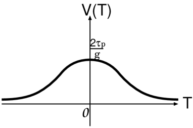
Figure 3.2: The potential $V(T)=\frac{2\tau_{p}}{g}e^{-|T|^{2}}$ for a $Dp+\overline{Dp}$ system

By the way the most interesting fact here is that this form of tachyon potential does not depend on what kind of closed string background we choose. This can be understood from eq.(3.5.1) because we have not used any information about the closed string background, which is included in $I_{0}$ in eq.(3.5.1). This fact is called universality of the tachyon potential [74]. The information of the closed string background is only included in the coefficient of the tachyon potential in eq.(3.5.1). This coefficient gives the mass of a $Dp+\overline{Dp}$ system, and this fact is physically desirable because the mass depends on the closed string background through the measure $\sqrt{-\det(G_{\mu\nu}-B_{\mu\nu})}$, which is just the Dirac-Born-Infeld factor.

Now let us consider the second conjecture of tachyon condensation [28, 29]. It is about the condensation of topologically nontrivial tachyons, not constant tachyons. In this case, as we have said in section 2.4, lower dimensional D-branes appear after tachyon condensation. Here we start from a $Dp+\overline{Dp}$ system, thus we expect that a non-BPS $D(p-1)$ brane or a BPS $D(p-2)$ brane is generated after the tachyon condensation.

In the same way as the verification of the first conjecture we set all the massive fields and two gauge fields $A^{\pm}_{\mu}(X)$ to zero in boundary action (3.3.71), and boundary action (3.3.71) becomes

$$I_{B} = \int_{\partial\Sigma}d\tau\left[\bar{\eta}\dot{\eta}-i\sqrt{\frac{2}{\pi}}\bar{\eta}\psi^{\mu}\partial_{\mu}T(X)+i\sqrt{\frac{2}{\pi}}\psi^{\mu}\eta\overline{\partial_{\mu}T}(X)+\frac{1}{2\pi}\bar{T}T(X)\right]$$ (3.5.3)

$$= \int_{\partial\Sigma}d\tau\left[-\frac{2}{\pi}(\psi^{\mu}\partial_{\mu}\bar{T}(X))\frac{1}{\partial_{\tau}}(\psi^{\nu}\partial_{\nu}T(X))+\frac{1}{2\pi}\bar{T}T(X)\right],$$

where in the second line we have eliminated $\eta(\tau)$ and $\bar{\eta}(\tau)$ by the Gaussian path integral, and $\frac{1}{\partial_{\tau}}$ is defined by

$$\frac{1}{\partial_{\tau}}f(\tau)=\int d\tau^{\prime}\epsilon(\tau-\tau^{\prime})f(\tau^{\prime}).$$ (3.5.4)

From the above expression it does not seem that we can exactly perform the path integral (3.3.75) to obtain the disk partition function because the boundary action is nonlinear. However if we restrict the tachyon field $T(X)$ to the linear order of $X^{\mu}$ this becomes the Gaussian path integral and is exactly solvable. The meaning of this restriction will be mentioned in section 3.8.

To perform the path integral let us expand $T(X)$ around the zero mode $x^{\mu}$ by using the relation $X^{\mu}(\tau)=x^{\mu}+\xi^{\mu}(\tau)$. $T(X)$ becomes

$$T(X)=T(x)+\xi^{\mu}\partial_{\mu}T(x)+\frac{1}{2}\xi^{\mu}\xi^{\nu}\partial_{\mu}\partial_{\nu}T(x)+\cdots\cdots.$$ (3.5.5)

If we restrict the tachyon field to the linear order, boundary action (3.5.3) becomes

$$I_{B} = \int_{\partial\Sigma}d\tau\left[\frac{1}{2\pi}\bar{T}T(x)-\frac{2}{\pi}(\partial_{\mu}\bar{T}\partial_{\nu}T(x))\psi^{\mu}\frac{1}{\partial_{\tau}}\psi^{\nu}+\frac{1}{2\pi}\xi^{\mu}\xi^{\nu}\partial_{\mu}\bar{T}\partial_{\nu}T(x)\right],$$ (3.5.6)

where we have used the equation $\int d\tau\xi^{\mu}(\tau)=0$ due to $\int d\tau X^{\mu}(\tau)=x^{\mu}$. This action includes only the second order of the fields $\xi^{\mu}(\tau)$ and $\psi^{\mu}(\tau)$, and path integral (3.3.75) for the disk partition function can exactly be performed as the Gaussian path integral.

Now let us move on to the concrete calculation of the disk partition function $Z$, which is the same as the action $S$ of string field theory. The difference from eq.(3.5.1) is that the calculation here depends on what kind of closed string background we choose. In generally curved closed string backgrounds it is difficult to perform the path integral (3.3.75) with bulk sigma model action (3.1.1). Therefore, from now on we will consider the flat background. The meaning of “flat” here is to set the closed string metric $G_{\mu\nu}$ and the NSNS B-field $B_{\mu\nu}$ to constant values, which satisfy the equation of motion of supergravity. Under this restriction the bulk action $I_{0}$ in eq.(3.1.1) is drastically simplified as

$$I_{0} = \frac{1}{4\pi}\int d^{2}z\Bigl{[}(G_{\mu\nu}+B_{\mu\nu})\partial X^{\mu}\bar{\partial}X^{\nu}$$ (3.5.7)

$$~{}~{}~{}~{}~{}~{}~{}~{}~{}~{}~{}~{}~{}~{}-i(G_{\mu\nu}+B_{\mu\nu})\psi^{\mu}_{L}\bar{\partial}\psi^{\nu}_{L}+i(G_{\mu\nu}-B_{\mu\nu})\psi^{\mu}_{R}\partial\psi^{\nu}_{R}\Bigr{]}.$$

In this case the action includes only the second powers of fields $(X^{\mu},~{}\psi^{\mu}_{L},~{}\psi^{\mu}_{R})$. Therefore the path integral of internal part of disk in eq.(3.3.75) can be performed as the Gaussian integral and the total expression of eq.(3.3.75) reduces to the path integral only on the boundary of disk, which is a one-loop diagram in the one-dimensional theory:

$$Z = \int[d^{10}xD\xi D\psi]\exp[-I^{\prime}_{B}(x,\xi,\psi)],$$ (3.5.8)

where

$$I^{\prime}_{B} = I_{B}+\frac{1}{8\pi}\int d\tau_{1}\int d\tau_{2}\xi^{\mu}(\tau_{1})\xi^{\nu}(\tau_{2})K^{-1}_{\mu\nu}(\tau_{1},\tau_{2})$$ (3.5.9)

$$~{}~{}~{}~{}~{}~{}~{}~{}+\frac{1}{2\pi}\int d\tau_{1}\int d\tau_{2}\psi^{\mu}(\tau_{1})\psi^{\nu}(\tau_{2})L^{-1}_{\mu\nu}(\tau_{1},\tau_{2}),$$

and

$$K^{-1}_{\mu\nu}(\tau_{1},\tau_{2}) = \frac{1}{2\pi}(G_{\mu\nu}-B_{\mu\nu})\sum^{\infty}_{m=1}me^{im(\tau_{1}-\tau_{2})}+\frac{1}{2\pi}(G_{\mu\nu}+B_{\mu\nu})\sum^{\infty}_{m=1}me^{-im(\tau_{1}-\tau_{2})},$$

$$L^{-1}_{\mu\nu}(\tau_{1},\tau_{2}) = \frac{i}{2\pi}(G_{\mu\nu}-B_{\mu\nu})\sum^{\infty}_{r=\frac{1}{2}}e^{ir(\tau_{1}-\tau_{2})}-\frac{i}{2\pi}(G_{\mu\nu}+B_{\mu\nu})\sum^{\infty}_{r=\frac{1}{2}}e^{-ir(\tau_{1}-\tau_{2})}.$$

The proof of this expression is given in appendix B. Note that $\psi^{\mu}$ obeys the anti-periodic boundary condition around the boundary of disk.

Inserting the explicit form of boundary action $I_{B}$ given in eq.(3.5.6) into eq.(3.5.9), the action $I^{\prime}_{B}$ becomes

$$I^{\prime}_{B} = \bar{T}T(x)+\frac{1}{8\pi}\int d\tau_{1}\int d\tau_{2}\xi^{\mu}(\tau_{1})\xi^{\nu}(\tau_{2})K^{\prime-1}_{\mu\nu}(\tau_{1},\tau_{2})$$ (3.5.11)

$$~{}~{}~{}~{}~{}~{}~{}~{}+\frac{1}{2\pi}\int d\tau_{1}\int d\tau_{2}\psi^{\mu}(\tau_{1})\psi^{\nu}(\tau_{2})L^{\prime-1}_{\mu\nu}(\tau_{1},\tau_{2}),$$

where

$$K^{\prime-1}_{\mu\nu}(\tau_{1},\tau_{2}) = \frac{1}{2\pi}\sum^{\infty}_{m=1}\{(G_{\mu\nu}-B_{\mu\nu})m+4\partial_{(\mu}\bar{T}\partial_{\nu)}T\}e^{im(\tau_{1}-\tau_{2})}$$

$$~{}~{}~{}~{}~{}~{}~{}~{}+\frac{1}{2\pi}\sum^{\infty}_{m=1}\{(G_{\mu\nu}+B_{\mu\nu})m+4\partial_{(\mu}\bar{T}\partial_{\nu)}T\}e^{-im(\tau_{1}-\tau_{2})},$$

$$L^{\prime-1}_{\mu\nu}(\tau_{1},\tau_{2}) = \frac{i}{2\pi}\sum^{\infty}_{r=\frac{1}{2}}\{(G_{\mu\nu}-B_{\mu\nu})+\frac{4}{r}\partial_{(\mu}\bar{T}\partial_{\nu)}T\}e^{ir(\tau_{1}-\tau_{2})}$$

$$~{}~{}~{}~{}~{}~{}~{}~{}-\frac{i}{2\pi}\sum^{\infty}_{r=\frac{1}{2}}\{(G_{\mu\nu}+B_{\mu\nu})+\frac{4}{r}\partial_{(\mu}\bar{T}\partial_{\nu)}T\}e^{-ir(\tau_{1}-\tau_{2})},$$

and $\partial_{(\mu}\bar{T}\partial_{\nu)}T$ denotes the symmetric part of $\partial_{\mu}\bar{T}\partial_{\nu}T$. From eq.(3.5.11) we can see that we have only to perform the Gaussian integral about the nonzero modes $\xi^{\mu}$ and $\psi^{\mu}$, which is the same calculation as that of the Coleman-Weinberg potential in field theory. The result is given by

$$S = Z\propto\int d^{p+1}xe^{-|T(x)|^{2}}\left[\frac{\prod^{\infty}_{r=\frac{1}{2}}-\det\{(G_{\mu\nu}-B_{\mu\nu})+\frac{4}{r}\partial_{(\mu}\bar{T}\partial_{\nu)}T\}}{\prod^{\infty}_{m=1}-\det\{(G_{\mu\nu}-B_{\mu\nu})m+4\partial_{(\mu}\bar{T}\partial_{\nu)}T\}}\right]$$ (3.5.13)

$$= \exp\Biggl{[}-\sum^{\infty}_{m=1}\ln\left[-\det\{(G_{\mu\nu}-B_{\mu\nu})m+4\partial_{(\mu}\bar{T}\partial_{\nu)}T\}\right]$$

$$~{}~{}~{}~{}~{}~{}~{}~{}~{}~{}~{}~{}+\sum^{\infty}_{r=\frac{1}{2}}\ln\left[-\det\{(G_{\mu\nu}-B_{\mu\nu})+\frac{4}{r}\partial_{(\mu}\bar{T}\partial_{\nu)}T\}\right]\Biggr{]},$$

$$= \exp\left[\ln\{-\det(G_{\mu\nu}-B_{\mu\nu})\}\left(-\sum^{\infty}_{m=1}e^{-\epsilon m}+\sum^{\infty}_{r=\frac{1}{2}}e^{-\epsilon r}\right)\right]$$

$$\times~{}~{}~{}\exp\left[-\sum^{\infty}_{m=1}{\rm Tr}\{\ln(m\delta^{\mu}_{\nu}+M^{\mu}_{~{}\nu})\}+\sum^{\infty}_{r=\frac{1}{2}}{\rm Tr}\left\{\ln\left(\delta^{\mu}_{~{}\nu}+\frac{1}{r}M^{\mu}_{~{}\nu}\right)\right\}\right],$$

where $e^{-\epsilon m}$ and $e^{-\epsilon r}$ are regulators to control the divergence, and the matrix $M^{\mu}_{~{}\nu}$ is given by

$$M^{\mu}_{~{}\nu}=4\left(\frac{1}{G-B}\right)^{\mu\rho}\partial_{(\rho}\bar{T}\partial_{\nu)}T.$$ (3.5.14)

Here by using the relation

$$-\sum^{\infty}_{m=1}e^{-2\epsilon m}+\sum^{\infty}_{r=\frac{1}{2}}e^{-2\epsilon r}=\frac{1}{2}+{\cal O}(\epsilon),$$ (3.5.15)

the first exponential becomes

$$\sqrt{-\det(G_{\mu\nu}-B_{\mu\nu})}.$$ (3.5.16)

This part gives the Dirac-Born-Infeld factor if we include the gauge field (see section 3.6).

The subtle calculation is in the second exponential of eq.(3.5.13). By expanding the logarithm the internal part of this exponential becomes

$${\displaystyle\sum^{\infty}_{\ell=1}} \frac{(-1)^{\ell-1}}{\ell}\left(-\sum^{\infty}_{m=1}\frac{1}{m^{\ell}}+\sum^{\infty}_{r=\frac{1}{2}}\frac{1}{r^{\ell}}\right){\rm Tr}M^{\ell}$$

$$= \left(-\sum^{\infty}_{m=1}\frac{e^{-\epsilon m}}{m}+\sum^{\infty}_{r=\frac{1}{2}}\frac{e^{-\epsilon r}}{r}\right){\rm Tr}M+\sum^{\infty}_{\ell=2}\frac{(-1)^{\ell-1}}{\ell}\left(-\sum^{\infty}_{m=1}\frac{1}{m^{\ell}}+\sum^{\infty}_{r=\frac{1}{2}}\frac{1}{r^{\ell}}\right){\rm Tr}M^{\ell}.$$

Here notice that the following relations hold:

$$-\sum^{\infty}_{m=1}\frac{e^{-\epsilon m}}{m}+\sum^{\infty}_{r=\frac{1}{2}}\frac{e^{-\epsilon r}}{r} = \lim_{\epsilon\rightarrow 0}\left[\ln(1-e^{-\epsilon})-\ln\frac{1-e^{-\frac{\epsilon}{2}}}{1+e^{-\frac{\epsilon}{2}}}\right]=\ln 4,$$ (3.5.18)

$$\sum^{\infty}_{m=1}\frac{1}{(m-\frac{1}{2})^{\ell}} = 2^{\ell}\left(\sum^{\infty}_{m=1}\frac{1}{m^{\ell}}-\sum^{\infty}_{m=1}\frac{1}{(2m)^{\ell}}\right)=(2^{\ell}-1)\zeta(\ell),$$ (3.5.19)

$$\ln\Gamma(z) = \sum^{\infty}_{\ell=2}\frac{(-1)^{\ell}}{\ell}\zeta(\ell)z^{\ell}-\gamma z-\ln z,$$ (3.5.20)

where $\zeta(\ell)$, $\Gamma(z)$ and $\gamma$ are the zeta function, the gamma function and the Euler’s constant, respectively. By using these relations we can obtain the final expression of the action of string field theory:

$$S=\frac{2\tau_{p}}{g}\int d^{p+1}xe^{-|T(x)|^{2}}\sqrt{-\det(G_{\mu\nu}-B_{\mu\nu})}Z(M),$$ (3.5.21)

where the total normalization is determined in the same way as eq.(3.5.2), and $Z(M)$ is given by

$$Z(M) = 4^{{\rm Tr}M}\frac{Z_{1}(M)^{2}}{Z_{1}(2M)},$$ (3.5.22)

$$Z_{1}(M) = \det\Gamma(M)e^{\gamma{\rm Tr}M}\det M.$$ (3.5.23)

If $\det M$ and $\det\Gamma(M)$ look singular, we have to go back to the definition by the trace formula (3.5.1), where they are well-defined.

Incidentally, to obtain this result we assumed that the tachyon field $T(X)$ has linear dependence of $X^{\mu}$. The linear configuration of the tachyon is generally written by

$$T(x)=a+\sum_{\mu=0}^{p}b_{\mu}x^{\mu},\ \ (a,b_{\mu}\in{\mathbf{C}}).$$ (3.5.24)

This can be put into the following form by a Poincaré transformation and U(1) gauge transformation in eq.(3.3.1)

$$T(x)=\frac{1}{2}(iu_{1}x_{1}+u_{2}x_{2}),\ \ (u_{1},u_{2}\in{\bf R}).$$ (3.5.25)

Indeed, this configuration of the tachyon field is desirable to obtain lower dimensional D-branes. For non-zero $u_{i}$ this represents a vortex in the $x^{1}$-$x^{2}$ plane. If $u_{1}=0$ or $u_{2}=0$, this corresponds to a kink configuration. This fact is easy to see if we insert this configuration into the tachyon potential $V(T)$

$$V(T)\propto e^{-|T(x_{1},x_{2})|^{2}}=e^{-\frac{1}{4}(u_{1}x_{1})^{2}-\frac{1}{4}(u_{2}x_{2})^{2}}.$$ (3.5.26)

From this we can see that if both $u_{1}$ and $u_{2}$ are nonzero the energy is almost zero in the $x^{1}$-$x^{2}$ plane except around $x^{1}=x^{2}=0$. In other words the energy localizes at $x^{1}=x^{2}=0$ with width $\left(\frac{1}{u_{1}},~{}\frac{1}{u_{2}}\right)$. This means that a codimension two soliton appears at $x^{1}=x^{2}=0$, which can be regarded as a BPS D$(p-2)$ brane. In the same way if $u_{1}$ is nonzero and $u_{2}$ is zero, a non-BPS D$(p-1)$ brane appears as a codimension one soliton at $x^{1}=0$.

Let us now condense the tachyon field under the simplest background $(G_{\mu\nu}=\eta_{\mu\nu},~{}B_{\mu\nu}=0)$. First we insert the tachyon profile (3.5.25) in the matrix $M$ in eq.(3.5.14). It is given by $M=\mbox{diag}(u_{1}^{2},~{}u_{2}^{2})$ and $Z(M)$ in eq.(3.5.22) becomes $Z(u_{1}^{2})Z(u_{2}^{2})$. Now according to the g-theorem, which was explained in section 3.2, the action $S$ of string field theory should monotonically decrease along the one-dimensional renormalization group flow. Indeed the function $\sqrt{\frac{2}{y}}Z(y)$ is a monotonically decreasing function of $y$, and it takes the minimum value at $y=\infty$ with its value

$$\sqrt{\frac{2}{y}}Z(y)\to\sqrt{2\pi}\ \ \ (y\to\infty).$$ (3.5.27)

Therefore there exist three decay modes $(u_{1},u_{2})=(\infty,0),\ (0,\infty),\mbox{and}\ (\infty,\infty)$, where the conformal invariance is restored. The first two cases represent kink configurations and the width $\frac{1}{u_{1}}$ (or $\frac{1}{u_{2}}$) of the kink goes to zero, which corresponds to the fact that the width of D-branes is zero. Therefore, we expect a non-BPS D$(p-1)$-brane will be generated at $x^{1}=0$ or $x^{2}=0$, respectively. This speculation is verified if one computes the tension and see that the correct value is reproduced as follows

$$S = \frac{2\tau_{p}}{g}\int d^{p}x\left(\int dx_{1}e^{-\frac{u_{1}^{2}}{4}x_{1}^{2}}\right)Z(u_{1}^{2})$$ (3.5.28)

$${\displaystyle\mathop{\longrightarrow}^{u_{1}\rightarrow\infty}} \frac{4\pi\tau_{p}}{g}\int d^{p}x=\frac{\sqrt{2}\tau_{p-1}}{g}\int d^{p}x~{}~{}~{}~{}~{}~{}~{}~{}(\mbox{for}~{}(u_{1},u_{2})=(\infty,0)).$$

Here we have used the relation $(2\sqrt{2}\pi)\tau_{p}=\tau_{p-1}$. The tension of a non-BPS D$(p-1)$ brane appears in the coefficient of the action.

More intuitive way to see the generation of a non-BPS D$(p-1)$-brane is to discuss the boundary interaction (3.3.71). Let us shift the original tachyon field by a real constant $T_{0}$ along $x^{1}$ as follows:

$$T(X)=\frac{1}{2}T_{0}+\frac{i}{2}u_{1}X_{1}.$$ (3.5.29)

The boundary interaction (3.3.71) after the condensation of the tachyon field (3.5.29) becomes

$$I_{B} = \int_{\partial\Sigma}d\tau\left[\bar{\eta}\dot{\eta}+\frac{1}{\sqrt{2\pi}}u_{1}\psi^{1}(\eta-\bar{\eta})+\frac{1}{8\pi}T_{0}^{2}+\frac{1}{8\pi}u_{1}^{2}(X^{1})^{2}+\cdot\cdot\cdot\right],$$ (3.5.30)

where the new tachyon field $T_{0}$ depends only on $X^{a}\ \ (a=0,2,\cdot\cdot\cdot,p)$. From this expression it is easy to see that in the limit $u_{1}\to\infty$ we can set $\eta=\bar{\eta}$ after we perform the path integral of the fermion $\psi^{1}$. The term $\cdot\cdot\cdot$ which depends on $A_{\mu}^{(-)}$ vanishes because it is proportional to $\bar{\eta}\eta\sim 0$. On the other hand, the gauge field $A_{\mu}^{(+)}$ is not sensitive to the tachyon condensation except that the element $A_{1}^{(+)}$ is no longer a gauge field and becomes a transverse scalar field since the boundary condition along $x^{1}$ becomes the Dirichlet one. Thus the final boundary action after integrating out the fields $X^{1}$ and $\psi^{1}$ is identified with that of a non-BPS D$(p-1)$-brane (3.3.90).

Next we turn to the case $(u_{1},u_{2})=(\infty,\infty)$. This corresponds to the vortex-type configuration and the width of the vortex $\left(\frac{1}{u_{1}},~{}\frac{1}{u_{2}}\right)$ goes to zero. Therefore, a BPS D$(p-2)$-brane is expected to be generated at $(x^{1},x^{2})=(0,0)$. This fact can also be checked by computing the tension as follows:

$$S = \frac{2\tau_{p}}{g}\int d^{p-1}x\left(\int dx_{1}dx^{2}e^{-\frac{u_{1}^{2}}{4}x_{1}^{2}-\frac{u_{2}^{2}}{4}x_{2}^{2}}\right)Z(u_{1}^{2})Z(u_{2}^{2})$$ (3.5.31)

$${\displaystyle\mathop{\longrightarrow}^{u_{1},u_{2}\rightarrow\infty}} \frac{8\pi^{2}\tau_{p}}{g}\int d^{p-1}x=\frac{\tau_{p-2}}{g}\int d^{p-1}x,$$

matching with the known result.

It is also interesting to consider multiple brane-antibrane systems. Let us consider $2^{k-1}$ pairs of brane-antibrane and condense the tachyon field (see the statement (2.4.79)). As an extension of the tachyon profile (3.5.25) the following configuration describes the tachyon condensation on multiple $Dp+\overline{Dp}$ systems:

$$T(x)=i\frac{u}{2}\sum_{\mu=1}^{2k}\Gamma^{\mu}x_{\mu},$$ (3.5.32)

where $\Gamma^{\mu}$ denotes $2^{k-1}\times 2^{k-1}$ $\Gamma$-matrix which belongs to $SO(2k)$ Clifford algebra. This configuration matches with the K-theory argument [11], which is a mathematical description of generation of D-brane charges. Equation (3.5.32) is known as the Atiyah-Bott-Shapiro construction [76] and a BPS D$(p-2k)$-brane is expected to be generated. This fact will become more explicit when we investigate the Wess-Zumino term in section 3.7. Moreover, in the same way as previous cases we can verify that the correct tension is produced if one starts with worldsheet action (3.3.85) for multiple brane-antibrane systems. Similarly one can also see that the condensation of the tachyon field

$$T(x)=i\frac{u}{2}\sum_{\mu=1}^{2k-1}\Gamma^{\mu}x_{\mu},$$ (3.5.33)

on $2^{k-1}$ $Dp+\overline{Dp}$ pairs produces a non-BPS D$(p-2k+1)$-brane.

3.5.2 On non-BPS D-branes

In this subsection we will consider the tachyon condensation on non-BPS D-branes [27]. It turns out to be very easy to describe it if we use the descent relation (2.3.3).

First the tachyon potential on a non-BPS D$p$-brane is obtained by using the result (3.5.2) for a $Dp+\overline{Dp}$ system and the descent relation (2.3.3). It is given by

$$V(T)=\frac{\sqrt{2}\tau_{p}}{g}e^{-\frac{T^{2}}{4}}.$$ (3.5.34)

The shape of potential is also the same as the one (fig. 3.2) for a $Dp+\overline{Dp}$ system except the normalization, and it does not depend on which kind of closed string background we choose [74].

Next we consider the condensation of a topologically nontrivial tachyon on a non-BPS D$p$-brane. To do this we need to obtain the action of string field theory for a non-BPS D$p$-brane. It is obtained from the result (3.5.21) for a $Dp+\overline{Dp}$ system by using the descent relation (2.3.3). For a non-BPS D-brane the result becomes simpler than that for a brane-antibrane system and it is given by

$$S=\frac{\sqrt{2}\tau_{p}}{g}\int d^{p+1}xe^{-\frac{T(x)^{2}}{4}}\sqrt{-\det(G_{\mu\nu}-B_{\mu\nu})}Z(y),$$ (3.5.35)

where

$$y = {\cal G}^{\mu\nu}\partial_{\mu}T\partial_{\nu}T~{}~{}~{}\mbox{with}~{}~{}~{}{\cal G}^{\mu\nu}=\left(\frac{1}{G-B}\right)^{(\mu\nu)},$$ (3.5.36)

$$Z(y) = 4^{y}\frac{Z_{1}(y)^{2}}{Z_{1}(2y)},$$ (3.5.37)

$$Z_{1}(y) = \Gamma(y)e^{\gamma y}y.$$ (3.5.38)

Here ${\cal G}^{\mu\nu}$ is called open string metric [8], which is familiar to noncommutative theorists.

In the same way as a $Dp+\overline{Dp}$ system we consider the linear profile of the tachyon field $T(X)$ under the simplest background $(G_{\mu\nu}=\eta_{\mu\nu},~{}B_{\mu\nu}=0)$. Indeed the action (3.5.35) can also be obtained by restricting the tachyon field $T(X)$ to the linear configuration in the worldsheet action (3.3.90) and performing the Gaussian path integral to calculate the disk amplitude. By using the Poincaré transformation the tachyon field becomes

$$T(x)=u_{1}x_{1}~{}~{}~{}(u_{1}\in{\bf R}).$$ (3.5.39)

Now we insert this into the action (3.5.35) and minimize it by taking the limit $u_{1}\rightarrow\infty$, which corresponds to the RG-flow going into the IR fixed point. The result becomes

$$S = \frac{\sqrt{2}\tau_{p}}{g}\int d^{p}x\left(\int dx_{1}e^{-\frac{u_{1}^{2}}{4}x_{1}^{2}}\right)Z(u_{1}^{2})$$ (3.5.40)

$${\displaystyle\mathop{\longrightarrow}^{u_{1}\rightarrow\infty}} 2\sqrt{2}\pi\frac{\tau_{p}}{g}\int d^{p}x=\frac{\tau_{p-1}}{g}\int d^{p}x.$$

From the coefficient we can see that the correct tension of a BPS D$(p-1)$ brane is generated.

Moreover because the action (3.5.35) is simpler than that for a brane-antibrane we are able to calculate the tachyon condensation under the nontrivial constant background $(G_{\mu\nu},~{}B_{\mu\nu})$. The parameter $y$ in eq.(3.5.36) becomes $y={\cal G}^{11}u_{1}^{2}$. Inserting this into the action (3.5.35) it becomes

$$S = \frac{\sqrt{2}\tau_{p}}{g}\int d^{p}x\left(\int dx_{1}e^{-\frac{u_{1}^{2}}{4}x_{1}^{2}}\right)\sqrt{-\det(G_{\mu\nu}-B_{\mu\nu})}Z({\cal G}^{11}u_{1}^{2})$$ (3.5.41)

$${\displaystyle\mathop{\longrightarrow}^{u_{1}\rightarrow\infty}} \frac{\tau_{p-1}}{g}\int d^{p}x\sqrt{-\det(G_{\mu\nu}-B_{\mu\nu})}\sqrt{{\cal G}^{11}}$$

$$= \frac{\tau_{p-1}}{g}\int d^{p}x\sqrt{-\det(G_{\alpha\beta}-B_{\alpha\beta})},$$

where indices $\alpha$ and $\beta$ do not include $1$. This means that the tension including the DBI factor is correctly reproduced after the tachyon condensation.

One can also see that the condensation of the tachyon field [12]

$$T(x)=i\frac{u}{2}\sum_{\mu=1}^{2k-1}\Gamma^{\mu}x_{\mu},$$ (3.5.42)

on $2^{k-1}$ non-BPS D$p$-branes produces a BPS D$(p-2k+1)$-brane.

In this way we have described all decay modes which can be handled in BSFT by free field calculations and they are all consistent with K-theoretic arguments [11, 12].

3.6 The Dirac-Born-Infeld Actions for Non-BPS Systems

As we already know, the effective action for a BPS D$p$-brane consists of two parts [77]. One is the Dirac-Born-Infeld term [78, 79, 33] and the other is the Wess-Zumino term [80, 81, 82]. The explicit form of these terms can be written as

$$S=\frac{\tau_{p}}{g}\int d^{p+1}x\sqrt{-\det(G_{\mu\nu}-B_{\mu\nu}+4\pi F_{\mu\nu})}+\tau_{p}\int C\wedge e^{4\pi F},$$ (3.6.1)

where $g$ is the string coupling constant. On the other hand the effective actions for non-BPS systems also have the same structure as eq.(3.6.1), and boundary string field theory enables us to calculate their explicit forms. The meaning of “effective” will be explained in section 3.8. In this section we will compute the Dirac-Born-Infeld type action with tachyons and gauge fields on non-BPS systems [28, 29, 34, 27, 32], and in section 3.7 we will calculate the Wess-Zumino terms.

In section 3.5 we obtained the target space actions (3.5.21) and (3.5.35) for a $Dp+\overline{Dp}$ system and for a non-BPS D$p$-brane without the gauge fields. Here we will obtain the world volume actions including the gauge fields on these systems.

First we will discuss the worldvolume action on a non-BPS D$9$-brane [26, 34, 83]. If we want to consider a non-BPS D$p$-brane we have only to perform the T-dual transformation to the worldvolume action by replacing one component of the gauge field with a transverse scalar. In the worldsheet action (3.3.90) for a non-BPS D9-brane the gauge field appears in the following way

$$I_{B} = \int_{\partial\Sigma}d\tau d\theta\left[\cdots-iD_{\theta}{\bf X}^{\mu}A_{\mu}({\bf X})+\cdots\cdots\right]$$ (3.6.2)

$$= \int_{\partial\Sigma}d\tau\left[\cdots-i\dot{X}^{\mu}A_{\mu}(X)+2iF_{\mu\nu}(X)\psi^{\mu}\psi^{\nu}+\cdots\cdots\right].$$

Since the fields $A_{\mu}(X)$ and $F_{\mu\nu}(X)$ nontrivially depend on the worldsheet field $X$, we can not exactly perform the path integral. However, if we restrict the field configuration of the gauge field to the constant field strength $F_{\mu\nu}$, this worldsheet action includes only the second order of the fields $X^{\mu}$ and $\psi^{\mu}$ as follows

$$I_{B}=-i\int_{\partial\Sigma}d\tau\left[\cdots-\frac{1}{2}X^{\mu}\dot{X}^{\nu}F_{\mu\nu}-2\psi^{\mu}\psi^{\nu}F_{\mu\nu}+\cdots\cdots\right].$$ (3.6.3)

From this expression we can see that by adding these terms to eq.(3.5.9) or eq.(3.5.11) the path integral (3.5.8) is equivalent to the description of replacing $B_{\mu\nu}$ with $\tilde{B}_{\mu\nu}\equiv B_{\mu\nu}-4\pi F_{\mu\nu}$ in eq.(3.5.1) or eq.(3.5.1) [33]. Indeed this combination satisfies the desired gauge invariance : $B_{\mu\nu}\rightarrow B_{\mu\nu}+\partial_{\mu}\zeta_{\nu}-\partial_{\nu}\zeta_{\mu},~{}A_{\mu}\rightarrow A_{\mu}+\frac{1}{4\pi}\zeta_{\mu}$.

Therefore the target space action for a non-BPS D9-brane is given by

$$S = \frac{\sqrt{2}\tau_{9}}{g}\int d^{10}xe^{-\frac{T(x)^{2}}{4}}\sqrt{-\det(G_{\mu\nu}-B_{\mu\nu}+4\pi F_{\mu\nu})}Z({\cal G}^{\mu\nu}\partial_{\mu}T\partial_{\nu}T)$$

$$= \frac{\sqrt{2}\tau_{9}}{g}\int d^{10}xe^{-\frac{T(x)^{2}}{4}}\sqrt{-\det(G_{\mu\nu}-B_{\mu\nu}+4\pi F_{\mu\nu})}\left(1+2(\ln 2){\cal G}^{\mu\nu}\partial_{\mu}T\partial_{\nu}T+\cdots\cdots\right),$$

where the definition of $Z(y)$ is given in eq.(3.5.37), and in the second line we have used its Taylor expansion given by

$$Z(y)=1+2(\ln 2)y+{\cal O}(y^{2}).$$ (3.6.5)

Here we can see the Dirac-Born-Infeld factor in the action [89]. We can apply this calculation to that for a BPS D-brane only if we set the tachyon field to zero (see appendix B or the paper [33]).

Note that this action is available only when $\partial_{\mu}\partial_{\nu}T=0$ and $\partial_{\rho}F_{\mu\nu}=0$. The tachyon profile (3.5.39) satisfies this condition, and the following configuration is indeed a solution to the equation of motion of the above action:

$$T(x)=u_{1}x_{1}~{}(u_{1}\rightarrow\infty),~{}~{}~{}A_{\mu}(x)=0.$$ (3.6.6)

Next we move on to the worldvolume action for a $D9+\overline{D9}$ system. In this case the situation is more complicated because two kinds of gauge fields appear in the action. In fact as we can see in the worldsheet action (3.3.71) for a brane-antibrane system, even if we consider the constant field strength $F^{+}_{\mu\nu}$ and $F^{-}_{\mu\nu}$ the sigma model is not an action with only free fields. The terms with $A^{+}_{\mu}$ includes only the second order of fields, while the terms with $A^{-}_{\mu}$ can not avoid including higher powers of the fields $X^{\mu}$ and $\psi^{\mu}$. If we include only the constant field strength $F^{+}_{\mu\nu}$ and set the other gauge field $A^{-}$ to zero, we have only to replace NSNS B-field $B_{\mu\nu}$ with $B_{\mu\nu}-4\pi F^{+}_{\mu\nu}$ in action (3.5.21).

On the other hand, we can show the general structure of the target space action for a brane-antibrane system. Here we set all the massive fields to zero in the worldsheet action (3.3.71) and consider the most general configuration, not the linear one, of the tachyon field and the gauge fields, which is different from the analysis in section 3.5. It is given by

$$S = \frac{\tau_{9}}{g}\int d^{10}xe^{-T\bar{T}(x)}\left[\sqrt{-\det\{G_{\mu\nu}-B_{\mu\nu}+4\pi F^{(1)}_{\mu\nu}(x)\}}\right.$$ (3.6.7)

$$~{}~{}~{}~{}~{}~{}~{}\left.+\sqrt{-\det\{G_{\mu\nu}-B_{\mu\nu}+4\pi F^{(2)}_{\mu\nu}(x)\}}+\sum_{n=1}^{\infty}{\cal{P}}_{2n}(F^{(i)}_{\mu\nu},T,\bar{T},D_{\rho})\right],$$

where ${\cal{P}}_{2n}$ is the $2n$-derivative term constructed from $F^{(i)}_{\mu\nu},T,\bar{T}$ and $2n$ covariant derivatives $D_{\mu}$. Note that, for example, $F_{\mu\nu}^{(-)}T$ is regarded as a 2-derivative term and should be included in ${\cal{P}}_{2}$ because of the identity $[D_{\mu},D_{\nu}]T=-iF_{\mu\nu}^{(-)}T$. This ambiguity is reminiscent of the case of the non-Abelian Dirac-Born-Infeld action [86] in which $[F_{\mu\nu},F_{\gamma\sigma}]=i[D_{\mu},D_{\nu}]F_{\gamma\sigma}$ should be regarded as a derivative term.

Here note that from the analysis in section 3.5 this action should have the following configurations of $T(x)$ and $A^{(1),(2)}_{\mu}(x)$ as exact solutions to the equation of motion of eq.(3.6.7):

$$T(x)=\frac{i}{2}u_{1}x_{1}~{}~{}~{}~{}~{}(u_{1}\rightarrow\infty),~{}~{}~{}~{}~{}~{}~{}~{}~{}~{}~{}~{}~{}~{}~{}~{}A^{(1)}_{\mu}=A^{(2)}_{\mu}=0,$$ (3.6.9)

$$T(x)=\frac{1}{2}(iu_{1}x_{1}+u_{2}x_{2})~{}(u_{1},u_{2}\rightarrow\infty),~{}~{}~{}A^{(1)}_{\mu}=A^{(2)}_{\mu}=0.$$

These solitonic solutions and eq.(3.6.6) can be interpreted as the field theoretical realization of the famous statement that “the D-branes are solitons in string theory”.

Now let us prove eq.(3.6.7). We use the matrix form of the world-sheet action (3.3.85):

$$S=Z=\int DXD\psi~{}{\rm exp}[-I_{0}(X,\psi)]~{}{\rm Tr\,P\,exp}\int^{\pi}_{-\pi}d\tau M(\tau),$$ (3.6.10)

where

$$M(\tau)=\left[\begin{array}[]{c c }i\dot{X}^{\mu}A^{(1)}_{\mu}-2i\psi^{\mu}\psi^{\nu}F^{(1)}_{\mu\nu}-\frac{1}{2\pi}T\bar{T}&~{}i\sqrt{\frac{2}{\pi}}\psi^{\mu}D_{\mu}T\\ -i\sqrt{\frac{2}{\pi}}\psi^{\mu}\overline{D_{\mu}T}{}&i\dot{X}^{\mu}A^{(2)}_{\mu}-2i\psi^{\mu}\psi^{\nu}F^{(2)}_{\mu\nu}-\frac{1}{2\pi}\bar{T}T\end{array}\right].$$

First we expand $X^{\mu}$ around the zero mode $x^{\mu}$ as $X^{\mu}(\tau)=x^{\mu}+\xi^{\mu}(\tau)$ and path integrate $\xi^{\mu}(\tau)$ and $\psi^{\mu}(\tau)$. From the expansion $T\bar{T}(X)=T\bar{T}(x)+\xi^{\mu}(\partial_{\mu}(T\bar{T}))(x)+\cdots=T\bar{T}(x)+\xi^{\mu}(D_{\mu}(T\bar{T}))(x)+\cdots$, we can replace $T\bar{T}(X)$ in $Z$ by $T\bar{T}(x)$ if we remove the derivative terms which can be included in ${\cal{P}}_{2n}$. The $F_{\mu\nu}^{(i)}(X)$ terms can also be replaced by $F_{\mu\nu}^{(i)}(x)$. Furthermore we see that the contributions from the off diagonal part of the matrix $M(\tau)$ have the form of ${\cal{P}}_{2n}$ since they can be expanded as $D_{\mu}T(X)=D_{\mu}T(x)+\xi^{\nu}(\partial_{\nu}(D_{\mu}T))(x)+\cdots$. The terms $i\dot{X}^{\mu}A_{\mu}^{(i)}(X)$ in the diagonal part are combined with the other non-gauge covariant terms to give gauge covariant ones. Therefore we conclude that the action for a brane-antibrane system becomes eq.(3.6.7).

Similarly, we can show that the action for $n$ $D9$-branes and $m$ $\overline{D9}$-branes becomes

$$S = \frac{\tau_{9}}{g}\int d^{10}x\left({\rm SymTr}\left[e^{-T\bar{T}}\sqrt{-\det\{G_{\mu\nu}-B_{\mu\nu}+4\pi F^{(1)}_{\mu\nu}\}}\right.\right.$$ (3.6.13)

$$\left.\left.+e^{-\bar{T}T}\sqrt{-\det\{G_{\mu\nu}-B_{\mu\nu}+4\pi F^{(2)}_{\mu\nu}\}}+\sum_{n=1}^{\infty}{\cal{P}}_{2n}(F^{(i)},T,\bar{T},D_{\mu})\right)\right],$$

where ${\rm SymTr}$ denotes the symmetrized trace for $T\bar{T},\bar{T}T$ and $F^{(i)}_{\mu\nu}$ [86]. Note that if we consider multiple $Dp+\overline{Dp}$ branes transverse scalars appear. Moreover it is known that complicated terms appear according to T-duality argument [87] in multi $Dp+\overline{Dp}$ systems.

At first glance these results may look false because it seems that massive modes which is exchanged between a D-brane and an anti D-brane modify the sum of the Dirac-Born-Infeld actions. However this effect comes from an open string one-loop diagram (cylinder amplitude) and in the disk amplitude this effect does not cause any modification.

Now we make another comment about the target space actions (LABEL:nonBPSaction11) and (3.6.7) (or (3.6.13)). From these actions we can see that the classical action completely vanishes after the constant tachyon condensation $T(x)=T\rightarrow\infty$. This fact indicates that open string degrees of freedom completely disappear after the tachyon condensation, and it coincides with the physical picture that D-branes disappear. On the other hand the vanishing of the action can not be explained by the simple field theory picture like the scalar QED or the Yang-Mills-Higgs theory, which we saw in section 2.4. In the usual field theory action [59] like $S=\int d^{10}x\left[F^{\mu\nu}F_{\mu\nu}+\partial^{\mu}T\partial_{\mu}T+V(T)\right]$ the kinetic terms remain after the tachyon condensation. In string field theory the kinetic term of the gauge field is given by $\frac{1}{g_{\scriptscriptstyle YM}^{2}}e^{-\frac{T^{2}}{4}}F^{\mu\nu}F_{\mu\nu}$ and it really vanishes. Here note that the effective coupling constant is given by

$$\frac{1}{g_{\scriptscriptstyle eff}^{2}}=\frac{1}{g_{\scriptscriptstyle YM}^{2}}e^{-\frac{T^{2}}{4}},$$ (3.6.14)

thus at $T\rightarrow\infty$ this becomes strong. Because of this property we could consider that the flux of the gauge field is confined to become closed string degrees of freedom [93, 91, 92, 90, 88, 89].

Moreover we can find another intriguing fact which the action like
$S=\int d^{10}x~{}{\rm Tr}\left[F^{\mu\nu}F_{\mu\nu}+D^{\mu}TD_{\mu}T+V(T)\right]$ can not explain. First we already know that the action (3.6.13) has the soliton solutions given by the Atiyah-Bott-Shapiro construction (3.5.32) and (3.5.33) with zero gauge fields:

$$T(x)=i\frac{u}{2}\sum_{\mu=1}^{2k-1}\Gamma^{\mu}x_{\mu}~{}~{}~{}~{}(u\rightarrow\infty),~{}~{}~{}~{}~{}~{}~{}~{}~{}~{}~{}~{}~{}~{}~{}~{}A^{(1)}_{\mu}=A^{(2)}_{\mu}=0,$$ (3.6.15)

$$T(x)=i\frac{u}{2}\sum_{\mu=1}^{2k}\Gamma^{\mu}x_{\mu}~{}~{}~{}~{}~{}(u\rightarrow\infty),~{}~{}~{}~{}~{}~{}~{}~{}~{}~{}~{}~{}~{}~{}~{}~{}A^{(1)}_{\mu}=A^{(2)}_{\mu}=0.$$ (3.6.16)

These solutions describe the decay of $D9+\overline{D9}$ systems to various lower dimensional D-branes. On the other hand, it is known that in usual field theories these kinds of solutions do not exist. In the field theory picture a non-BPS D$8$-brane can be regarded as a kink solution in the field theory on $D9+\overline{D9}$ systems. A BPS D$7$-brane is a vortex in it. In fact these solutions can be found as approximate solutions in the truncated action which ignores terms with more than three derivatives [71, 72]. However, the Atiyah-Bott-Shapiro type solution is generally prohibited in standard local field theories. Indeed, according to the Derrick’s theorem [95] in local field theories, there do not exist more than codimension $5$ solitons because the total energy of these solutions often diverge. Codimension $4$ solitons are instantons, which are BPS-solutions in the four-dimensional Yang-Mills theory, and they can be realized as BPS D0-branes on BPS D4-branes [94, 80]. However, the Atiyah-Bott-Shapiro type solutions represent not only less than codimension $4$ but also more than codimension 5 solitons like the decay of multi $D9+\overline{D9}$ systems to a BPS D3-brane (codimension 6) or to a BPS D1-brane (codimension 8). These solutions can not be found in standard local field theories. The existence of higher codimensional solitons is one of features in string field theories, which are nonlocal.

Finally we will compute the action for a brane-antibrane system as a sigma model partition function perturbatively up to $\alpha^{\prime 2}$ under the simplest background $(G_{\mu\nu}=\eta_{\mu\nu},~{}B_{\mu\nu}=0)$. Hereafter we will restore the dimension-full parameter $\alpha^{\prime}$ by including a factor $\alpha^{\prime}/2$. From eq.(3.5.9) and eq.(3.5.1) we can obtain the Green functions of $\xi^{\mu}(\tau)$ and $\psi^{\mu}(\tau)$ as follows:

$$\langle\xi^{\mu}(\tau)\xi^{\mu}(\tau^{\prime})\rangle = \alpha^{\prime}\!\!\!\sum_{m\in{\mathbf{Z}\neq 0}}\!\!\frac{1}{|m|}e^{im(\tau-\tau^{\prime})-\epsilon|m|}=2\alpha^{\prime}\!\!\!\sum_{m\in{\mathbf{Z}>0}}\!\!\frac{1}{m}{\rm cos}(m(\tau-\tau^{\prime}))e^{-\epsilon|m|},$$ (3.6.17)

$$\langle\psi^{\mu}(\tau)\psi^{\mu}(\tau^{\prime})\rangle = -\frac{i}{2}\sum_{r\in{\mathbf{Z}}+\frac{1}{2}}\frac{r}{|r|}e^{ir(\tau-\tau^{\prime})-\epsilon|r|}=\sum_{m\in{\mathbf{Z}+\frac{1}{2}>0}}{\rm sin}(r(\tau-\tau^{\prime}))e^{-\epsilon|r|}.$$ (3.6.18)

The regularization used here keeps the world-sheet supersymmetry and the spacetime gauge invariance (3.3.1) or (3.3.3), which corresponds to world-sheet global symmetry [31, 30]. The expansion of fields in eq.(3.3.83) are given by

$$T\bar{T}(X) = T\bar{T}(x)+\xi^{\mu}(D_{\mu}(T\bar{T}))(x)+\cdots+\frac{1}{4!}\xi^{\sigma}\xi^{\rho}\xi^{\nu}\xi^{\mu}(D_{\sigma}D_{\rho}D_{\nu}D_{\mu}(T\bar{T}))(x)+\cdots,$$

$$A^{(i)}_{\mu}(X) = A^{(i)}_{\mu}(x)+\xi^{\nu}\partial_{\nu}A^{(i)}_{\mu}(x)+\cdots,\hskip 14.22636ptF^{(i)}_{\mu\nu}(X)=F^{(i)}_{\mu\nu}(x)+\xi^{\rho}(D_{\rho}F^{(i)}_{\mu\nu})(x)+\cdots,$$

$$D_{\mu}T(X) = D_{\mu}T(x)+\xi^{\nu}(\partial_{\nu}(D_{\mu}T))(x)+\frac{1}{2}\xi^{\rho}\xi^{\nu}(\partial_{\rho}\partial_{\nu}(D_{\mu}T))(x)+\cdots.$$ (3.6.19)

Now we can compute the partition function by the perturbation about $\alpha^{\prime}$. Since the concrete computation is somewhat complicate, we will show only the result:

$$S=Z = \frac{\tau_{9}}{g}\int d^{10}xe^{-\bar{T_{R}}T_{R}}\left[2+8\alpha^{\prime}(\log 2)D^{\mu}T_{R}\overline{D_{\mu}T_{R}}+\alpha^{\prime 2}\pi^{2}\left(F^{(1)\mu\nu}_{R}F^{(1)}_{R\mu\nu}+F^{(2)\mu\nu}_{R}F^{(2)}_{R\mu\nu}\right)\right.$$ (3.6.20)

$$\hskip 56.9055pt+4\alpha^{\prime 2}\gamma_{0}(D^{\mu}D^{\nu}T_{R})(D_{\mu}D_{\nu}\overline{T}_{R})+32\alpha^{\prime 2}i(\log 2)^{2}F^{(-)\mu\nu}_{R}D_{\mu}T_{R}D_{\nu}\overline{T}_{R}$$

$$\hskip 56.9055pt+2\alpha^{\prime 2}\left(8(\log 2)^{2}-\frac{1}{3}\pi^{2}\right)(D^{\mu}T_{R}D_{\mu}\overline{T}_{R})^{2}$$

$$\hskip 56.9055pt-\alpha^{\prime 2}\frac{2}{3}\pi^{2}(D^{\mu}T_{R}D_{\mu}T_{R})(D^{\nu}\overline{T}_{R}D_{\nu}\overline{T}_{R})$$

$$\hskip 56.9055pt+\frac{\pi^{2}}{6}\alpha^{\prime 2}\left((D^{\mu}D^{\nu}T_{R})\overline{T}_{R}+T_{R}(D^{\mu}D^{\nu}\overline{T}_{R})\right)$$

$$\hskip 56.9055pt\left.\;\;\;~{}~{}\times\left(D_{\mu}D_{\nu}(\overline{T}_{R}T_{R})+D_{\nu}\overline{T}_{R}D_{\mu}T_{R}+D_{\mu}\overline{T}_{R}D_{\nu}T_{R}\right)+\cdots\right],$$

where $\gamma_{0}$ is a constant which is defined by

$$\gamma_{0}={\rm\lim_{\epsilon\rightarrow 0}}\left(\sum_{r,m>0}\frac{1}{m}\left(\frac{1}{r+m}+\frac{1}{r-m}\right)e^{-(r+m)\epsilon}-(\log\epsilon)^{2}\right),$$ (3.6.21)

and we have renormalized the tachyon field and the gauge field as

$$T = T_{R}+\alpha^{\prime}(\log\epsilon)D^{\mu}D_{\mu}T_{R}+\frac{1}{2}\alpha^{\prime 2}(\log\epsilon)^{2}D^{\mu}D_{\mu}D^{\nu}D_{\nu}T_{R}$$

$$~{}~{}~{}~{}~{}~{}~{}~{}~{}~{}~{}~{}~{}~{}~{}~{}+i\alpha^{\prime 2}(\log\epsilon)^{2}D^{\mu}F_{R\mu\nu}^{(-)}D^{\nu}T_{R},$$

$$A_{\mu}^{(-)} = A_{R\mu}^{(-)}+\alpha^{\prime}(\log\epsilon)D^{\nu}F_{R\nu\mu}^{(-)}.$$ (3.6.22)

Note that the above equation can also be regarded as a field redefinition of the target space fields from $T(x),~{}A_{\mu}(x)$ to $T_{R}(x),~{}A_{R\mu}(x)$. We can see that the renormalization in the worldsheet corresponds to the field redefinition in the target space [8].

3.7 The Wess-Zumino Terms for Non-BPS Systems

In this section we will compute the Wess-Zumino terms (RR-couplings or Chern-Simon terms) on non-BPS D-branes and brane-antibrane systems within the framework of BSFT [28, 29]. These terms for non-BPS systems correspond to the second term of the effective action for a BPS D-brane in eq.(3.6.1). The boundary string field theory enable us to calculate these terms in the same way as the calculation of the Dirac-Born-Infeld type actions.

The difference in the computations from the previous sections is that the result is completely exact without any assumptions that the tachyon is the linear order or something. Furthermore the resulting expression has a intriguing mathematical structure known as superconnection [53]. This fact was already conjectured in [11, 96] for brane-antibrane systems. Here we can see the explicit proof of this in BSFT and we point out that this structure can also be found in the Wess-Zumino terms on non-BPS D-branes. These results give another evidence of classification of D-brane charges by K-theory[13, 14, 11, 12].

In this section we consider $D9+\overline{D9}$ systems and non-BPS D$9$-branes. If we would like to obtain the result for $Dp+\overline{Dp}$ systems or non-BPS D$p$-branes, we have to replace several components of the gauge field with transverse scalars due to the T-duality. However, we have to note that they also include other nontrivial terms called Myers terms [87]. In our original paper [28] we also obtained the complete forms of Myers terms, while in this thesis we omit them.

3.7.1 Calculations and results

Here we start with the simplest flat background $(G_{\mu\nu}=\eta_{\mu\nu},~{}B_{\mu\nu}=0)$, and instead we put a little RR-flux in the background. In this case we can deal with the shift of the background by perturbation from the flat background. In BSFT this shift can be realized by inserting a RR vertex operator inside the disk.

The important thing here is that the picture [97] of the RR-vertex operator should be $(-\frac{1}{2},-\frac{3}{2})$. This is because we consider the insertion of only one RR-vertex operator and the total picture number on the disk should be $-2$. The RR vertex operator with $(-\frac{1}{2},-\frac{3}{2})$ picture is given by [98]

$$V^{(-\frac{1}{2},-\frac{3}{2})} = e^{-\frac{1}{2}\phi_{L}-\frac{3}{2}\phi_{R}}(P_{-}\hat{C})^{AB}S_{LA}S_{RB},$$

$$\hat{C}^{AB} = \sum_{p:{\scriptscriptstyle odd~{}(even)}}\frac{1}{p!}(\Gamma^{\mu_{1}\cdot\cdot\cdot\mu_{p}})^{AB}C_{\mu_{1}\cdot\cdot\cdot\mu_{p}},$$ (3.7.1)

where $\phi_{L}$ and $\phi_{R}$ denote the bosonized superconformal ghosts of left-moving and right-moving sectors, respectively. We define $S_{LA}$ and $S_{RB}$ as spin-fields constructed from world-sheet fermions and $P_{-}$ denotes the projection of the chirality $\frac{1-\Gamma_{11}}{2}$. The index $p$ in $\sum_{p}$ runs odd integers for Type IIA and even integers for Type IIB. For more details of the notation for spinors see appendix A.2.

According to the construction of BSFT in section 3.2 we can separate the matter part from the ghost part and we have only to consider the contribution from the matter to calculate the disk partition function. Therefore from now on we will ignore the ghost part. Anyway the most important thing is that the coefficient $C_{\mu_{1}\cdot\cdot\cdot\mu_{p}}$ of the RR-vertex operator represents a RR p-form gauge field [98], not the field strength $F_{\mu_{1}\cdot\cdot\cdot\mu_{p}}$, since the coefficient of a RR-vertex operator with standard $(-\frac{1}{2},-\frac{1}{2})$ picture is the field strength [99] and this does not appear in the Wess-Zumino terms.

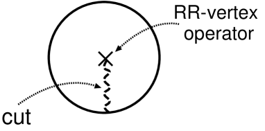
Figure 3.3: A RR-vertex operator inserted inside the disk generates the cut. Because of this cut worldsheet fermions on the boundary of disk take the periodic boundary condition $\psi^{\mu}(\tau+2\pi)=\psi^{\mu}(\tau)$.

First we turn to a $D9+\overline{D9}$ system and determine the Wess-Zumino term up to its overall normalization. The important thing we have to notice is that the contribution from nonzero modes of $X^{\mu}$ completely cancels out that from nonzero modes of $\psi^{\mu}$, and only the contribution from zero modes remains. This fact comes from the worldsheet supersymmetry. Indeed all fermions at the boundary of disk obey the periodic boundary condition $\psi^{\mu}(\tau+2\pi)=\psi^{\mu}(\tau)$ due to the cut generated by a RR vertex operator (see figure 3.3), and the worldsheet supersymmetry is completely preserved in the one-dimensional boundary theory. Therefore one can believe that the contribution from fermions and bosons is canceled with each other for nonzero-modes [28, 29].

As an example, we can see the cancellation of the contribution from nonzero modes in eq.(3.5.13). Since the worldsheet fermions take the periodic boundary condition in this case, its mode-index runs positive integer numbers. If we replace the positive half-integer index $r$ with the positive integer index $n$ in eq.(3.5.13), we can see that the contribution from bosons completely cancels out that from fermions in eq.(3.5.15) and eq.(3.5.1).

However, in eq.(3.5.13) we assumed that the tachyon field $T(X)$ is linear and we also set the gauge field strength $F_{\mu\nu}(X)$ to a constant or zero. In this section we do not even assume that approximation. What we would like to insist is that even under the general dependence of $X$ in $T(X)$ and $F_{\mu\nu}(X)$, the contribution from non-zero modes disappears. Unfortunately its explicit proof is very difficult.

If we admit this fact, the calculation of the Wess-Zumino terms reduces to that of only the zero modes of the boson ($x^{\mu}$) and the fermions ($\psi_{0}^{\mu}$ and $\eta,\bar{\eta}$). In this calculation it is better to change the path integral formalism into the Hamiltonian formalism. The procedure is the same as that for obtaining equation (3.3.83) in subsection 3.3.2. The path integral of the boundary fermions $\eta$ and $\bar{\eta}$ can be represented by the RR-sector analog of the important formula (3.3.85):

$$\int D\eta D\bar{\eta}\ e^{-I_{B}}=\mbox{Tr P}\ (-1)^{F}\ \exp\ \int_{-\pi}^{\pi}d\tau M(\tau),$$ (3.7.2)

$$M(\tau)=\left(\begin{array}[]{cc}i\dot{X}^{\mu}A^{(1)}_{\mu}-2i\psi^{\mu}\psi^{\nu}F^{(1)}_{\mu\nu}-\frac{1}{2\pi}T\bar{T}&i\sqrt{\frac{2}{\pi}}\psi^{\mu}D_{\mu}T\\ -i\sqrt{\frac{2}{\pi}}\psi^{\mu}\overline{D_{\mu}T}&i\dot{X}^{\mu}A^{(2)}_{\mu}-2i\psi^{\mu}\psi^{\nu}F^{(2)}_{\mu\nu}-\frac{1}{2\pi}\bar{T}T\end{array}\right),$$ (3.7.5)

where the insertion of $(-1)^{F}(=[\bar{\eta},\eta])$ is due to the periodic boundary condition of $\eta$ and $\bar{\eta}$, and it can be replaced with the Pauli matrix $\sigma_{3}$ in the same reason as the statement above eq.(3.3.85). Since we have only to take the zero modes into account, we can perform the following replacement in eq.(3.7.2)

$$X^{\mu}(\tau)\rightarrow x^{\mu}~{}~{},~{}~{}\psi^{\mu}(\tau)\rightarrow\psi^{\mu}_{0}=\frac{1}{\sqrt{2}}i^{\frac{1}{2}}\Gamma^{\mu},$$ (3.7.6)

where the factor $i^{\frac{1}{2}}$ is due to the conformal map from the open string picture to the closed string picture [100]. Because of this replacement $\tau$ dependence is dropped out of eq.(3.7.2) and we can regard the path-ordered trace Tr P as an ordinary trace. Thus, we have obtained

$$\int D\eta D\bar{\eta}DXD\psi~{}e^{-I_{0}-I_{B}}=\mbox{Str}:\exp\left(\begin{array}[]{cc}2\pi F_{\mu\nu}^{(1)}\Gamma^{\mu}\Gamma^{\nu}-T\bar{T}&2i^{\frac{3}{2}}\sqrt{\pi}\Gamma^{\mu}D_{\mu}T\\ -2i^{\frac{3}{2}}\sqrt{\pi}\Gamma^{\mu}\overline{D_{\mu}T}&2\pi F_{\mu\nu}^{(2)}\Gamma^{\mu}\Gamma^{\nu}-\bar{T}T\end{array}\right):,$$ (3.7.9)

where the supertrace Str is defined to be a trace with insertion of $\sigma_{3}$, and the symbol $:\ :$ means that $\Gamma$-matrices are antisymmetrized because operators should be normal-ordered in the Hamiltonian formalism.

After we insert the RR-vertex operator (3.7.1) and take the trace using the famous relation (A.2.19) between the Clifford algebra (A.2.18) and the differential forms (A.2.17) (see appendix A.2), we can easily obtain the final expression of the Wess-Zumino term on a $D9+\overline{D9}$ system [29, 28]:

$$S=\tau_{9}\ \mbox{Str}\ \int C\wedge\exp\left(\begin{array}[]{cc}2\pi\alpha^{\prime}F^{(1)}-T\bar{T}&i^{\frac{3}{2}}\sqrt{2\pi\alpha^{\prime}}\ DT\\ -i^{\frac{3}{2}}\sqrt{2\pi\alpha^{\prime}}\ \overline{DT}&2\pi\alpha^{\prime}F^{(2)}-\bar{T}T\end{array}\right),$$ (3.7.12)

where we have recovered $\alpha^{\prime}=2$. Here the total normalization was determined as follows. If we set the tachyon field $T$ to zero the above action becomes

$$\tau_{9}\ \int C\wedge e^{2\pi\alpha^{\prime}F^{(1)}}-\tau_{9}\ \int C\wedge e^{2\pi\alpha^{\prime}F^{(2)}}.$$ (3.7.13)

This should be the sum of the Wess-Zumino terms for a BPS D9-brane and an BPS antiD9-brane, and the total normalization should be equal to that for a BPS D9-brane, which is given in eq.(3.6.1).

The non-abelian generalization is also straightforward if the above abelian supertrace is replaced with the non-abelian one:

$$\mbox{Str diag}(a_{1},a_{2},\cdot\cdot\cdot,a_{N},b_{1},b_{2},\cdot\cdot\cdot,b_{M})=\sum_{i=1}^{N}a_{i}-\sum_{j=1}^{M}b_{j},$$ (3.7.14)

where we have assumed that there are $N$ D$9$-branes and $M$ antiD$9$-branes.

Next we will calculate the Wess-Zumino term for non-BPS D$9$-branes. In the same way as the previous sections it is easily obtained by using the descent relation (2.3.3) and (2.3.73). According to this rule the Chan-Paton degrees of freedom $1,\sigma_{1},\sigma_{2}$ and $\sigma_{3}$ reduce to only $1$ and $\sigma_{1}$. The other difference appears in the fermion number operator $(-1)^{F}$ in eq.(3.7.2). It is represented by $(-1)^{F}=\eta\simeq\frac{1}{\sqrt{2}}\sigma_{1}$ in the case of a non-BPS D9-brane because in the Hamiltonian formalism the quantization of the boundary fermion $\eta$ is given by $\eta^{2}=\frac{1}{2}$. Thus up to the overall factor $\mu^{\prime}$ the result is given by:

$$S = \mu^{\prime}\ \mbox{Tr}\ \left[\ \int C\wedge\exp{\left[-\frac{1}{4}T^{2}-\sqrt{\pi\alpha^{\prime}}i^{\frac{3}{2}}DT\sigma_{1}+2\pi\alpha^{\prime}F\right]}\sigma_{1}\right],$$ (3.7.15)

$$= i\mu^{\prime}\ \mbox{Tr}\int C\wedge\exp{\left[-\frac{1}{4}T^{2}-\sqrt{\pi\alpha^{\prime}}i^{\frac{1}{2}}DT+2\pi\alpha^{\prime}F\right]}_{odd},$$

where the trace Tr in the first equation involves the degree of freedom of the Pauli matrix $\sigma_{1}$. The covariant derivative of a Hermitian tachyon field on non-BPS D-branes is denoted by $DT=dT-i[A,T]$. Also note that in the second expression only the terms which include odd powers of $DT$ should be picked up because of the trace with respect to $\sigma_{1}$, and therefore we have represented this prescription by $]_{odd}$ .

The normalization $\mu^{\prime}$ can not be determined in the same way as eq.(3.7.12) because if we set the tachyon field to zero this action completely vanishes. Instead it can be determined by the calculation of the S-matrix between a RR-field and a tachyon field since eq.(3.7.15) includes the coupling $\int C\wedge dT$ [101], and the result is given by

$$\mu^{\prime}=i^{\frac{1}{2}}\tau_{9}.$$ (3.7.16)

In this way we have derived the explicit Wess-Zumino terms on $\mbox{D9}+\overline{\mbox{D9}}$ systems and non-BPS D$9$-branes in BSFT. The important point is that one can read off the Wess-Zumino terms if one extracts the fermionic zero modes from the boundary action $I_{B}$. This may be said as a boundary topological model which naturally leads to the notion of superconnection as we will see in the next subsection. Note also that the above results can be applied to general D$p$-branes if the transverse scalars are set to zero. If we would like to include transverse scalars, the new terms called Myers terms appear in the action. For details see our original paper [28].

3.7.2 Superconnection and K-theory charge

Here we will discuss the interpretation of the Wess-Zumino terms on non-BPS D-branes and brane-antibrane systems as superconnections [53]. For brane-antibrane systems this fact was first suggested in [11]. A definite relation between the Wess-Zumino terms and the Chern character of the superconnection was proposed in the paper [96]. Our calculations in the previous subsection show that this interpretation indeed holds within the framework of BSFT as we will see below. Moreover we will argue that such an interpretation can be applied to non-BPS D-branes and our previous calculations give evidence for this. If one is interested in the index theorem and the anomaly related to the superconnections, see the papers [29, 102, 103].

Let us first review the definition and properties of superconnections following [53]. There are two kinds of superconnections: one is for even-cohomology and the other is for odd-cohomology. In the K-theoretic language the former is related to $K^{0}(M)$ and the latter to $K^{1}(M)$, where $M$ is a manifold regarded as the world-volume of D-branes. Both are defined as follows:

Superconnection for $K^{0}(M)$

In this case we consider a ${\mathbf{Z}}_{2}$-graded vector bundle $E=E^{(0)}\oplus E^{(1)}$, which can be directly applied to a brane-antibrane system if one identifies $E^{(0)}$ and $E^{(1)}$ as vector bundles on the branes and antibranes, respectively. The endomorphism $X\in\mbox{End}\ E$ of this superbundle has the following ${\mathbf{Z}}_{2}$-grading:

$$\mbox{deg}(X)=\left\{\begin{array}[]{c}\ 0\ \ \mbox{if}\ X:E^{(0)}\to E^{(0)}\ \mbox{or}\ E^{(1)}\to E^{(1)},\\ \ 1\ \ \mbox{if}\ X:E^{(0)}\to E^{(1)}\ \mbox{or}\ E^{(1)}\to E^{(0)}.\end{array}\right.$$ (3.7.19)

In addition, there is also a natural ${\mathbf{Z}}$-grading if one considers the algebra of differential forms $\Omega(M)=\oplus\Omega^{p}(M)$, where $\Omega^{p}(M)$ denotes the algebra of $p$-forms on $M$. The crucial observation is to mix these two gradings and to define the ${\mathbf{Z}}_{2}$-grading for $\alpha\in\Omega^{p}(M,\mbox{End}\ E)=\Omega^{p}(M)\otimes\Omega^{0}(M,\mbox{End}\ E)$ as follows:

$$\alpha=\omega\otimes X\in\Omega^{p}(M)\otimes\Omega^{0}(M,\mbox{End}\ E),\ \ \mbox{deg}(\alpha)\equiv p+\mbox{deg}(X),$$ (3.7.20)

where $\Omega^{0}(M,\mbox{End}\ E)$ denotes the space of sections of $\mbox{End}\ E$. Under this definition its superalgebra is given by the following rule:

$$(\omega\otimes X)(\eta\otimes Y)=(-1)^{\mbox{deg}(X)\cdot\mbox{deg}(\eta)}\ (\omega\eta\otimes XY),$$ (3.7.21)

and the supercommutator can be defined as:

$$[\alpha,\beta]=\alpha\beta-(-1)^{\mbox{deg}(\alpha)\cdot\mbox{deg}(\beta)}\beta\alpha.$$ (3.7.22)

An element of $\Omega^{p}(M,\mbox{End}\ E)$ can be written as a $2\times 2$ matrix, where the diagonal elements and off-diagonal elements have even and odd degree of $\Omega^{0}(M,\mbox{End}\ E)$, respectively. We also define the supertrace as

$$\alpha\in\Omega(M,\mbox{End}\ E)=\left(\begin{array}[]{cc}\alpha_{1}&\alpha_{2}\\ \alpha_{3}&\alpha_{4}\end{array}\right),\ \ \ \mbox{Str}(\alpha)=\mbox{Tr}(\alpha_{1})-\mbox{Tr}(\alpha_{4})\in\Omega(M),$$ (3.7.25)

where Tr denotes the ordinary trace on vector bundles. Note that the supertrace of supercommutators vanishes.

Let us now define a superconnection on $E$ as an operator ${\mathcal{D}}=d+{\mathcal{A}}$ on $\Omega(M,\mbox{End}\ E)$ with odd degree satisfying the derivation property:

$${\mathcal{D}}(\omega\phi)=(d\omega)\phi+(-1)^{deg(\omega)}\omega({\mathcal{D}}\phi),\ \ \ \ \omega\in\Omega(M),\ \ \phi\in\Omega(M,\mbox{End}\ E).$$ (3.7.26)

For local calculations familiar to physicists one can regard ${\mathcal{A}}$ as a degree odd element of $\Omega(M,\mbox{End}\ E)$:

$${\mathcal{D}}=d+{\mathcal{A}}=\left(\begin{array}[]{cc}d+A^{(1)}&\sqrt{2\pi i}T\\ \sqrt{2\pi i}\bar{T}&d+A^{(2)}\end{array}\right),$$ (3.7.29)

where the factor $\sqrt{2\pi i}$ has been included for later convenience. The diagonal parts $d+A^{(1)}$ and $d+A^{(2)}$ denote the ordinary gauge connections of vector bundles $E^{(1)}$ and $E^{(2)}$, respectively. $T$ denotes an odd degree endomorphism of $E$. Notice that in this definition the exterior derivative $d$ does anti-commute with any odd elements in $\mbox{End}\ E$.

The curvature ${\mathcal{F}}$ of the superconnection ${\mathcal{D}}$ is defined as an even degree element of $\Omega(M,\mbox{End}\ E)$:

$${\mathcal{F}} = {\mathcal{D}}^{2}=d{\mathcal{A}}+{\mathcal{A}}^{2}$$ (3.7.32)

$$= \left(\begin{array}[]{cc}F^{(1)}+2\pi iT\bar{T}&\sqrt{2\pi i}DT\\ \sqrt{2\pi i}D\bar{T}&F^{(2)}+2\pi i\bar{T}T\end{array}\right),$$

where we have defined $DT=dT+A^{(1)}T+TA^{(2)}$.

The “even Chern character” of this superconnection is given by

$$\mbox{Str}\exp\left(\frac{i}{2\pi}{\mathcal{D}}^{2}\right)=\mbox{Str}\exp\left(\frac{i}{2\pi}{\mathcal{F}}\right).$$ (3.7.33)

It is easy to see that this is closed because

$$d\ (\mbox{Str}{\mathcal{D}}^{2n})=\mbox{Str}[{\mathcal{D}},{\mathcal{D}}^{2n}]=0.$$ (3.7.34)

Furthermore as shown in the main theorem in the paper [53], its cohomology class does not depend on the choice of $T$. Therefore that Chern character becomes

$$\mbox{Str}\exp\left(\frac{i}{2\pi}{\mathcal{D}}^{2}\right)\simeq\mbox{ch}(E_{1})-\mbox{ch}(E_{2})\in H^{even}(M,{\mathbf{Q}})\cong K^{0}(M),$$ (3.7.35)

where $\mbox{ch}(E)$ denotes the ordinary Chern character and we have applied the Chern isomorphism, which states that the even cohomology and the K-group $K^{0}(M)$ are equivalent if ${\mathbf{Q}}$ is tensored [11, 104]. Note that the difference of the Chern characters is seen in eq.(3.7.13).

Superconnection for $K^{1}(M)$

The first step to define the second superconnection is to regard a bundle $E$ as a module over the Clifford algebra $C_{1}={\mathbf{C}}\oplus{\mathbf{C}}\sigma_{1}$. In other words, we define the endomorphism of this superbundle as $\mbox{End}_{\sigma}\ E=\mbox{End}\ E\otimes C_{1}$. Let us call all elements which include $\sigma_{1}$ degree odd and the others degree even. In the physical context these correspond to the fields on non-BPS D-branes which belong to the GSO odd and even sector, respectively. The supertrace on $\mbox{End}_{\sigma}E$ is defined as follows:

$$\mbox{Tr}_{\sigma}(X+Y\sigma_{1})=2\mbox{Tr}(Y),$$ (3.7.36)

where $X,Y\in\mbox{End}_{\sigma}\ E$ are degree even elements. Further we mix the degree of differential forms in the same way as in the previous case (3.7.20),(3.7.21) and (3.7.22).

The superconnection on $E$ is locally defined as an odd element as follows

$${\mathcal{D}}=d+{\mathcal{A}}=d+A-\sqrt{\frac{i\pi}{2}}T\sigma_{1},$$ (3.7.37)

where $A$ is an ordinary connection and $T$ is a self-adjoint endomorphism. The curvature of this is also defined as

$${\mathcal{F}} = {\mathcal{D}}^{2}=d{\mathcal{A}}+{\mathcal{A}}^{2}$$ (3.7.38)

$$= F-\sqrt{\frac{i\pi}{2}}DT\sigma_{1}-\frac{i\pi}{2}T^{2},$$

where we have defined $DT=dT-i[A,T]$. The “odd Chern character” is given by

$$\mbox{Tr}_{\sigma}\exp\left(\frac{i}{2\pi}{\mathcal{D}}^{2}\right)=\mbox{Tr}_{\sigma}\exp\left(\frac{i}{2\pi}{\mathcal{F}}\right).$$ (3.7.39)

The main theorem in [53] again tells us that this character is closed and its cohomology class does not depend on the choice of $T$. Further we can regard this as an element of K-theory group $K^{1}(M)$:

$$\mbox{Tr}_{\sigma}\exp\left(\frac{i}{2\pi}{\mathcal{D}}^{2}\right)\ \in\ H^{odd}(M,{\mathbf{Q}})\cong K^{1}(M).$$ (3.7.40)

Physical interpretation

The role of superconnections in the D-brane physics is obvious if one notes that the Wess-Zumino terms on $D9+\overline{\mbox{D9}}$ systems and non-BPS D9-branes can be expressed as wedge products of RR-fields and the Chern characters of superconnections:

$$S = \tau_{9}\ \mbox{Str}\ \int_{M}\ C\wedge\exp\left({\frac{i}{2\pi}\mathcal{F}}\right)\ \ \ \ \ \ \mbox{(for a D9-$\overline{\mbox{D9}}$ )},$$ (3.7.41)

$$S = i^{\frac{1}{2}}\tau_{9}\ \mbox{Tr}_{\sigma}\ \int_{M}\ C\wedge\exp\left({\frac{i}{2\pi}\mathcal{F}}\right)\ \ \ \mbox{(for a non-BPS D9-brane)},$$ (3.7.42)

where the curvature ${\mathcal{F}}$ in the first equation represents the superconnection for $K^{0}(M)$ and in the second for $K^{1}(M)$. One can transform these mathematical expressions (3.7.32) and (3.7.38) into the physical ones (3.7.12) and (3.7.15) by following the prescription:

$$D=d+A \to 2\pi\sqrt{\alpha^{\prime}}D=2\pi\sqrt{\alpha^{\prime}}(d-iA).$$ (3.7.43)

Now, by using the Wess-Zumino terms we can verify the conjecture of tachyon condensation. If we consider a constant tachyon field the Wess-Zumino terms completely vanish due to the overall factor $e^{-|T|^{2}}$ or $e^{-\frac{1}{4}T^{2}}$, and this is consistent with the conjecture. The next channel of tachyon condensation is the case when the tachyon fields are topologically nontrivial. As we have said in section 3.6, the linear tachyon profiles in eq.(3.6.9) and eq.(3.6.9) are exact solutions to the equation of motion of the Dirac-Born-Infeld type action for a $D9+\overline{D9}$ system, and eq.(3.6.6) is an exact solution for a non-BPS D9-brane. By inserting these solutions we can see that the correct RR-charges are generated. For example by putting the linear tachyon solution (3.6.9) into the Wess-Zumino term (3.7.12) for a $D9+\overline{D9}$ system it becomes

$$\tau_{9}\int_{D7}C\wedge\left(\int dx_{1}dx_{2}~{}2\pi u_{1}u_{2}~{}e^{-\frac{1}{4}(u_{1}^{2}x_{1}^{2}+u_{2}^{2}x_{2}^{2})}\right)$$ (3.7.44)

$$= \tau_{9}\int_{D7}C\wedge\left(2\pi u_{1}u_{2}~{}\times\frac{(2\sqrt{\pi})^{2}}{u_{1}u_{2}}\right)=\tau_{7}\int_{D7}C,$$

where we have used the relation $(2\sqrt{2}\pi)^{2}\tau_{9}=\tau_{7}$. The coefficient in front of the last line just represents the charge of a BPS D$7$-brane. In the other cases of tachyon condensation we can see the correct RR-charges are generated. Especially if we consider the tachyon condensation with a higher codimensional soliton configuration like decay of $D9+\overline{D9}$ systems to a BPS D$3$ brane, we have only to use the Wess-Zumino term for multiple non-BPS systems and its solution given by the Atiyah-Bott-Shapiro construction [76] like eq.(3.5.32).

By the way, in the above calculation the most interesting thing is that we have not taken the limit $u_{1},~{}u_{2}\rightarrow\infty$ to obtain the RR-charge of a D7-brane. The finite value of $u_{1}$ or $u_{2}$ corresponds to the off-shell region. This observation means that D-brane charges are quantized even during tachyon condensation and are not altered by smooth deformation of the tachyon configuration. This is consistent with the fact that D-brane charges are determined by the even or odd Chern characters in eq.(3.7.33) and eq.(3.7.39) and that these values belong to the even or odd cohomology element. Note that the result of eq.(3.7.44) holds only when both $u_{1}$ and $u_{2}$ are nonzero. If either is zero, the configuration of the tachyon is trivial and one can not regard $T$ as an element in the desirable endomorphism.

In this way we can relate D-brane charges in the Wess-Zumino terms to other D-brane charges due to tachyon condensation. Especially we have found that all kinds of BPS D$(2p+1)$-brane charges in Type IIB theory are generated by starting from only $D9+\overline{D9}$ systems and considering its tachyon condensation [11]. On the other hand all kinds of BPS D$(2p)$-brane charges in Type IIA theory are produced by only non-BPS $D9$-branes [12]. Another important point is that the Chern characters which appear in the Wess-Zumino terms belong to the K-group $K^{0}(M)$ for $D9+\overline{D9}$ branes and $K^{1}(M)$ for non-BPS D9-branes. Therefore, these results are consistent with the already known fact in the paper [13, 14] that $K^{0}(M)$ classifies all kinds of BPS D$(2p+1)$-brane charges in Type IIB theory and $K^{1}(M)$ does all kinds of BPS D$(2p)$-brane charges in Type IIA theory. In this sense we can even consider that $D9+\overline{D9}$ systems and non-BPS D$9$-branes include all kinds of (BPS and non-BPS) D-brane configurations and might be regarded as the fundamental objects in string theory.

On the other hand there exists the other idea that all kinds of D-branes are made up of the lowest dimensional D-branes, like BFSS matrix theory. If we combine this idea with the K-theoretical argument, we could regard $D(-1)+\overline{D(-1)}$ systems and non-BPS $D(-1)$-branes as the most fundamental objects in Type IIA and IIB theories, and we could even consider their worldvolume theories as the nonperturbative definition of total string theory [105, 106, 107].

Anyway, this is the conclusion obtained from the K-theory argument.

3.8 The Meaning of Calculations in Boundary String Field Theory

In this section we will explain the meaning of the calculations of BSFT we have done. As we said in section 3.4, in general we can not perform calculations of BSFT if we include massive terms in the sigma model action. Thus, we have restricted the terms only to renormalizable ones. Moreover, when we construct BSFT in section 3.2, we set all terms with worldsheet ghosts to zero in the boundary action $I_{B}$. From these a natural question occurs : what exactly does the action $S$ which we have computed mean?

Firstly we will answer the question by considering the result (3.6.7) as an example. What we can assert is that the action (3.6.7) is regarded as an on-shell effective action for $T$ and $A_{\mu}$ in which the massive modes are integrated out, or an off-shell action obtained by setting the fields other than $T$ and $A_{\mu}$ to zero. However, if the one-point function of massive fields vanishes in all the off-shell region, we can regard this action as the off-shell effective action in which the massive fields are integrated out.

Here we will explain the above statement. First we will introduce the notion of integrating out massive fields. Let us imagine that we included all massive fields in the sigma model action and could obtain the classical action $S[T,A_{\mu},\upsilon^{\alpha}]$, where $\upsilon^{\alpha}~{}(\alpha=1,2,\cdots)$ denote all massive fields. In the quantum string field theory the effective action $S_{\scriptscriptstyle eff}[T,A_{\mu}]$ in which all massive fields are integrated out is defined by

$$e^{-S_{\scriptscriptstyle eff}[T,A_{\mu}]}=\int\left(\prod_{\alpha}D\upsilon^{\alpha}\right)e^{-S[T,A_{\mu},\upsilon^{\alpha}]}.$$ (3.8.45)

Of course this path integral includes loop calculations, thus to obtain the complete effective action we need to know the quantum framework of BSFT. However, if we consider the classical theory this path integral reduces to the lowest order of WKB approximation, which is the same as inserting a solution to equation of motion into the classical action $S[T,A_{\mu},\upsilon^{\alpha}]$ and deleting $\upsilon^{\alpha}$. Since we are considering the classical BSFT, this is just the meaning of integrating out massive fields and obtaining the effective action.

Now let us expand the classical action $S[T,A_{\mu},\upsilon^{\alpha}]$ by the massive fields $\upsilon^{\alpha}$:

$$S[T,A_{\mu},\upsilon^{\alpha}]=S^{(0)}[T,A_{\mu}]+\upsilon^{\alpha}S^{(1)}_{\alpha}[T,A_{\mu}]+\frac{1}{2}\upsilon^{\alpha}\upsilon^{\beta}S^{(2)}_{\alpha\beta}[T,A_{\mu}]+\cdots\cdots.$$ (3.8.46)

In general we can not obtain an exact solution to the equation of motion of $\upsilon^{\alpha}$. However, if the coefficient $S^{(1)}_{\alpha}[T,A_{\mu}]$ in the above equation vanishes, we can easily see that $\upsilon^{\alpha}=0$ is a solution and we can regard $S^{(0)}[T,A_{\mu}]$ as the effective action in which the massive fields are integrated out. On the other hand $S^{(0)}[T,A_{\mu}]$ is just the action which we are able to calculate from the renormalizable sigma model action. Therefore the crucial point is whether $S^{(1)}_{\alpha}[T,A_{\mu}]$ does vanish or not. Note that $S^{(1)}[T,A_{\mu}]=\frac{\partial S}{\partial\upsilon^{i}}|_{\upsilon^{i}=0}$ is equal to the one-point functions of the massive fields on the disk.

Indeed if we consider an open string background with the conformal invariance we can easily see that these one-point functions of massive fields vanish. Therefore the starting prescription of setting all massive fields to zero in the sigma model is the same as classically integrating them out in the target space action. This is the meaning of “on-shell effective action” in which massive fields are integrated out, although on-shell actions do not include any other information than S-matrices and are not useful.

The important point is whether these one-point functions vanish even in the off-shell region or not, which is nontrivial. In the cubic string field theory (CSFT) [15, 16] or Berkovits’ formalism [17] one point functions do not vanish and we have to include massive modes to obtain the correct answers. However, in BSFT from the success and correctness of the tachyon condensation in section 3.5 we guess that above facts hold in the case of the sigma model action with only free fields. Therefore if the above facts hold not only for the free sigma model but also for the generally renormalizable one (eq.(3.3.69) or eq.(3.3.90)), $S^{(1)}[T,A_{\mu}]$ vanishes in the off-shell region and we can regard eq.(3.6.7) as the off-shell effective action in which all massive modes are integrated out. On the other hand the Wess-Zumino terms might be regarded as off-shell effective actions because the results are completely exact and topological. However, we can not assert that these predictions are actually true. Now we have finished explaining the statement in the second paragraph of this section.

Finally we make a comment about the validity of the Dirac-Born-Infeld action (3.6.1) for a BPS D-brane and the action (LABEL:nonBPSaction11) for a non-BPS D-brane. To obtain these actions we assumed $\partial_{\mu}\partial_{\nu}T=\partial_{\rho}F_{\mu\nu}=0$ and set the closed string background to the flat one $(\partial_{\rho}G_{\mu\nu}=\partial_{\rho}B_{\mu\nu}=0)$. These results are based on the framework of BSFT. A natural question is what occurs if we ignore these constraints and examine these actions as pure field theories. Indeed there have been a lot of reports that these actions are valid beyond this approximation (for example see the papers [77, 78, 108, 87, 83]). This is one of mysterious facts in the relation between string theory and field theory.

Chapter 4 On-Shell Description of Tachyon Condensation

In the last chapter we have discussed tachyon condensation in the off-shell formalism of string theory - string field theory. In this chapter we will deal with tachyon condensation by using the on-shell string theory, which is just the conventional first-quantized string theory. We only need the knowledge of the conformal field theory, and especially we use the boundary state formalism, which was explained in chapter 2.

Historically the method in this chapter had been used [47, 46, 42, 39, 40, 37, 38, 44, 45] before the string field theory approach was found. The physical situation in this chapter is special and a little complicated, thus we think that this chapter is easily understood after the explanation of the general off-shell formalism.

4.1 Set Up

In this chapter we pick up a case of tachyon condensation which we can deal with by the conformally invariant technique called marginal deformation. We consider a $D2+\overline{D2}$ system in the flat space background and put the $\overline{D2}$-brane on top of the D2-brane. In this situation, as we saw in the previous chapter, there appears a tachyon in the spectrum of an open string between the D2-brane and the $\overline{D2}$-brane and off-shell tachyon condensation starts. However, here we consider a little different situation : we compactify the world volumes of the D2-branes on a two-dimensional torus $T^{2}$ and switch on $Z^{2}$ Wilson line on the $\overline{D2}$-brane along each direction of the torus $T^{2}$.

Let us express this situation by using the boundary state technique which was explained in chapter 2. First note that the world volumes of D2-branes are compactified on torus $T^{2}$ and the structure of the zero mode part of boundary states becomes a little complicated as we saw in eq.(2.1.19). If we put a D2-brane which is spread in $x^{1}$ and $x^{2}$ directions at $x^{i}=0~{}(i=3\sim 9)$, the zero mode part of its boundary state can be written as

$$|D2,\gamma\rangle^{0}_{\scriptscriptstyle NSNS} = \delta^{7}(x)\sum_{(w_{\scriptscriptstyle X}^{1},w_{\scriptscriptstyle X}^{2})\in{\bf Z}^{2}}|{\bf w_{\scriptscriptstyle X}},{\bf 0}\rangle,$$

$$|D2,\gamma\rangle^{0}_{\scriptscriptstyle RR} = \delta^{7}(x)\sum_{(w_{\scriptscriptstyle X}^{1},w_{\scriptscriptstyle X}^{2})\in{\bf Z}^{2}}|{\bf w_{\scriptscriptstyle X}},{\bf 0}\rangle\otimes|\Omega 2_{\scriptscriptstyle X},\gamma\rangle^{0}_{\scriptscriptstyle RR}.$$ (4.1.1)

The second important element in this chapter is to add $Z^{2}$ Wilson line in $x^{1}$ and $x^{2}$ directions only on the anti D2-brane. The general Wilson line which appears in the boundary state has already been explained in eq.(2.1.19), while $Z^{2}$ Wilson line means that the boundary state of the anti D2-brane has the phase factor with $Z^{2}$ periodicity $(-1)^{w_{\scriptscriptstyle X}^{1}+w_{\scriptscriptstyle X}^{2}}$.

Now we have to check whether there are any tachyonic modes in open strings between the D2-brane and the anti D2-brane. Let us see the open string spectrum by calculating the vacuum amplitude $\langle\overline{D2}|\Delta|D2\rangle$ and transforming it to the open partition function. The result is the same as that in eq.(2.3.62) except the explicit form of open string Hamiltonian, which is written as

$$L_{0} = 2\left(p^{0}p_{0}+\sum_{i=3}^{9}p^{i}p_{i}+M^{2}\right),$$

where

$$M^{2} = \sum_{\alpha=1,2}\frac{1}{R^{2}_{\alpha}}\left(n^{\alpha}+\frac{1}{2}\right)^{2}+(\mbox{nonzero modes})+\left\{\begin{array}[]{c}-\frac{1}{4}~{}~{}(\mbox{for NS})\\ 0~{}~{}(\mbox{for R})\end{array}\right.,$$ (4.1.4)

and $R_{1},R_{2}$ are radii of the torus $T^{2}$. From this expression we can see that the momenta in $x^{1}$ and $x^{2}$ directions are discretized in such a way that they are labeled by half integer numbers $n^{\alpha}+\frac{1}{2}~{}~{}(n^{\alpha}\in{\bf Z})$. This is because the boundary condition of the open string at one end obeys the unusual antiperiodic boundary condition, which is just caused by the effect of $Z^{2}$ Wilson line. From this mass spectrum $M^{2}$ of open strings with the opposite GSO-projection (see eq.(2.3.62)) we can see that the “tachyon” which we called before corresponds to a particle with its mass square

$$M^{2} = \left(\frac{n^{1}+\frac{1}{2}}{R_{1}}\right)^{2}+\left(\frac{n^{2}+\frac{1}{2}}{R_{2}}\right)^{2}-\frac{1}{4}.$$ (4.1.5)

From this equation the tachyon has the following Fourier modes

$$T(x^{1},x^{2})=\sum_{n^{1},n^{2}\in{\bf Z}^{2}}T_{n^{1}+\frac{1}{2},n^{2}+\frac{1}{2}}\exp\left\{{i\left(\frac{n^{1}+\frac{1}{2}}{R_{1}}\right)x^{1}+i\left(\frac{n^{2}+\frac{1}{2}}{R_{2}}\right)x^{2}}\right\}.$$ (4.1.6)

Especially $T_{\pm\frac{1}{2},\pm\frac{1}{2}}$ have the lowest mass square

$$M^{2}=\frac{1}{4}\left(\frac{1}{R_{1}^{2}}+\frac{1}{R_{2}^{2}}-1\right).$$ (4.1.7)

From this equation we can predict an interesting fact about stability of the brane-antibrane system, which can not be seen unless we switch on $Z^{2}$ Wilson line. It is the fact that whether the modes $T_{\pm\frac{1}{2},\pm\frac{1}{2}}$ have the positive or negative mass square depends on the size of torus $T^{2}$ which the D2-branes wind on. If the torus $T^{2}$ is large enough to satisfy $\frac{1}{R_{1}^{2}}+\frac{1}{R_{2}^{2}}<1$, $T_{\pm\frac{1}{2},\pm\frac{1}{2}}$ are tachyonic in the usual sense. This system becomes unstable and decays to something. However, if $\frac{1}{R_{1}^{2}}+\frac{1}{R_{2}^{2}}\geq 1$, $T_{\pm\frac{1}{2},\pm\frac{1}{2}}$ become massive and tachyonic modes completely disappear. This means that the brane-antibrane system becomes perturbatively stable.

This situation is quite different from that of the last chapter. Especially we can find that in some region of the parameter space $(R_{1},R_{2})$ the conformal invariance is not broken even if $|T|$ gets any expectation values. This is the case when $\frac{1}{R^{2}_{1}}+\frac{1}{R_{2}^{2}}$ is equal to $1$ and the modes $T_{\pm\frac{1}{2},\pm\frac{1}{2}}$ become massless. In that case the tachyon potential becomes completely flat, which means that the energy does not decrease or not increase if the tachyon has an expectation value. Therefore, we can consider that $T_{\pm\frac{1}{2},\pm\frac{1}{2}}$ plays the same role as one component of the gauge field $A^{\mu}(x)$ and we can regard the expectation value of $T_{\pm\frac{1}{2},\pm\frac{1}{2}}$ as the Wilson line like $a^{\alpha}$ in eq.(2.1.19). The method of shifting the background in the conformally invariant manner by switching on parameters like Wilson lines is called marginal deformation. Especially the process of a massless “tachyon” getting an expectation value is called marginal tachyon condensation.

However, there is a technically subtle point to perform the marginal deformation. This is because the vertex operator corresponding to massless elements $T_{\pm\frac{1}{2},\pm\frac{1}{2}}$ has a complicated form if we express it by using worldsheet fields $(X^{\mu}(z,\bar{z}),~{}\psi^{\mu}(z))$. Therefore, at first glance we can not understand how to incorporate the tachyon field as a Wilson line correctly.

4.2 The Vertex Operators of Marginal Tachyons

To see the technical subtlety mentioned above and to solve its problem let us choose the case $R_{1}=R_{2}=\sqrt{2}$ to satisfy $\frac{1}{R_{1}^{2}}+\frac{1}{R_{2}^{2}}=1$ and consider the condensation of the following linear combination of massless elements in eq.(4.1.6)

$$T_{1}(x^{1},x^{2}) \propto e^{i\frac{1}{2\sqrt{2}}(x^{1}+x^{2})}-e^{-i\frac{1}{2\sqrt{2}}(x^{1}+x^{2})},$$

$$T_{2}(x^{1},x^{2}) \propto -ie^{i\frac{1}{2\sqrt{2}}(x^{1}-x^{2})}+ie^{-i\frac{1}{2\sqrt{2}}(x^{1}-x^{2})}.$$ (4.2.8)

If we replace $x^{1},x^{2}$ with $X^{1}(z,\bar{z}),X^{2}(z,\bar{z})$ these become the vertex operators with $(-1)$-picture in terms of worldsheet superconformal ghost number [97].

According to this the corresponding open string vertex operators with 0-picture are written as

$$V_{T1} \propto (\psi^{1}+\psi^{2})(e^{i\frac{1}{2\sqrt{2}}(X^{1}+X^{2})}+e^{-i\frac{1}{2\sqrt{2}}(X^{1}+X^{2})})\otimes\sigma_{1},$$

$$V_{T2} \propto (\psi^{1}-\psi^{2})(e^{i\frac{1}{2\sqrt{2}}(X^{1}-X^{2})}+e^{-i\frac{1}{2\sqrt{2}}(X^{1}-X^{2})})\otimes\sigma_{2},$$ (4.2.9)

where we have assigned Chan-Paton factors $\sigma_{1}$ and $\sigma_{2}$ to $V_{T1}$ and $V_{T2}$.

The marginal deformation is to consider the coherent shift from the original background in the conformally invariant manner. To explain this let us consider the general boundary state (2.2.55) with the operator $e^{\alpha V_{T1}+\beta V_{T2}}$ acting on it. Here $\alpha$ and $\beta$ are the parameters which represent the vacuum expectation values of the tachyon fields $T_{1}$ and $T_{2}$ in eq.(4.2). However, this is a complicated form to deal with because as we can see in eq.(4.2) both $V_{T1}$ and $V_{T2}$ include exponentialized forms of $X^{1,2}(z,\bar{z})$ and double exponentials appear in $e^{\alpha V_{T1}+\beta V_{T2}}$. Thus, to make it an easy form let us change the worldsheet fields $(X^{\mu}(z,\bar{z}),~{}\psi^{\mu}_{L}(z),~{}\psi^{\mu}_{R}(\bar{z}))$ into more convenient ones [39, 42]. First let us rotate the coordinates by $\frac{\pi}{4}$

$$\begin{array}[]{rclrcl}Y^{1}&=&\frac{1}{\sqrt{2}}(X^{1}+X^{2}),&\ \ \ Y^{2}&=&\frac{1}{\sqrt{2}}(X^{1}-X^{2}),\\ &&&&&\\ \chi^{1}_{\scriptscriptstyle L(R)}&=&\frac{1}{\sqrt{2}}(\psi^{1}_{\scriptscriptstyle L(R)}+\psi^{2}_{\scriptscriptstyle L(R)}),&\ \ \ \chi^{2}_{\scriptscriptstyle L(R)}&=&\frac{1}{\sqrt{2}}(\psi^{1}_{\scriptscriptstyle L(R)}-\psi^{2}_{\scriptscriptstyle L(R)}).\end{array}$$

In this coordinate the radii of the torus $T^{2}$ become 1 in both $Y^{1}$ and $Y^{2}$ directions. This special radius enables us to use the method of bosonization and fermionization as follows

$$\tau_{i}\otimes C^{i}_{\scriptscriptstyle Y}(\pm 1,0)~{}e^{\pm iY^{i}_{\scriptscriptstyle L}}=\frac{1}{\sqrt{2}}(\xi^{i}_{\scriptscriptstyle L}\pm i\eta^{i}_{\scriptscriptstyle L}), \tau_{i}\otimes C^{i}_{\scriptscriptstyle Y}(0,\pm 1)~{}e^{\pm iY^{i}_{\scriptscriptstyle R}}=\frac{1}{\sqrt{2}}(\xi^{i}_{\scriptscriptstyle R}\pm i\eta^{i}_{\scriptscriptstyle R}),$$

$$\tilde{\tau}_{i}\otimes C^{i}_{\phi}(\pm 1,0)~{}e^{\pm i\phi^{i}_{\scriptscriptstyle L}}=\frac{1}{\sqrt{2}}(\xi^{i}_{\scriptscriptstyle L}\pm i\chi^{i}_{\scriptscriptstyle L}), \tilde{\tau}_{i}\otimes C^{i}_{\phi}(0,\pm 1)~{}e^{\pm i\phi^{i}_{\scriptscriptstyle R}}=\frac{1}{\sqrt{2}}(\xi^{i}_{\scriptscriptstyle R}\pm i\chi^{i}_{\scriptscriptstyle R}),$$ (4.2.10)

where there appear two types of cocycle factors. These cocycle factors must be put in to guarantee their correct statistics and correct (anti)commutation relations to various fields. One type is $\tau_{i}$ and $\tilde{\tau}_{i}~{}(i=1,2)$ [42, 40] and we also assume that $\chi^{i}_{L,R}$ and $\eta^{i}_{L,R}$ have the cocycle factors $\tau_{3}$ and $\tilde{\tau}_{3}$. The other type of cocycle factor is $C^{i}_{\scriptscriptstyle Y}(k^{i}_{\scriptscriptstyle YL},k^{i}_{\scriptscriptstyle YR})$ and $C^{i}_{\phi}(k^{i}_{\phi{\scriptscriptstyle L}},k^{i}_{\phi{\scriptscriptstyle R}})$, which are defined by [99]

$$C^{i}_{\scriptscriptstyle Y}(k^{i}_{\scriptscriptstyle YL},k^{i}_{\scriptscriptstyle YR})\equiv\exp\left[\frac{1}{2}\pi i(k^{i}_{\scriptscriptstyle YL}-k^{i}_{\scriptscriptstyle YR})(\hat{p}^{i}_{\scriptscriptstyle YL}+\hat{p}^{i}_{\scriptscriptstyle YR})\right].$$ (4.2.11)

Especially in the later calculations and proofs this second type of cocycle factor becomes crucial.

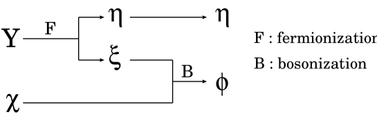
Figure 4.1: Two steps of bosonization

Now we have changed the coordinate system from $(Y^{i},\chi^{i}_{L(R)})$ to $(\phi^{i},\eta^{i}_{L(R)})$ by the bosonization technique (see figure 4.1). The operator product expansions (OPE) among these new fields can be obtained from those of old ones:

$$Y^{i}_{L}(z)Y^{j}_{L}(0)\sim-\delta_{ij}{\mbox{ln}}z Y^{i}_{R}(\bar{z})Y^{j}_{R}(0)\sim-\delta_{ij}{\mbox{ln}}\bar{z},$$ ,

$$\xi_{L}^{i}(z)\xi_{L}^{j}(0)\sim\delta_{ij}\frac{i}{z} \xi_{R}^{i}(\bar{z})\xi_{R}^{j}(0)\sim-\delta_{ij}\frac{i}{\bar{z}},$$ ,

$$\eta_{L}^{i}(z)\eta_{L}^{j}(0)\sim\delta_{ij}\frac{i}{z} \eta_{R}^{i}(\bar{z})\eta_{R}^{j}(0)\sim-\delta_{ij}\frac{i}{\bar{z}}.$$ , (4.2.12)

Also the following identities are useful:

$$\eta_{L}^{i}\xi_{L}^{i}=i\partial Y^{i}_{L} \eta_{R}^{i}\xi_{R}^{i}=-i\bar{\partial}Y^{i}_{R},$$ ,

$$\chi_{L}^{i}\xi_{L}^{i}=i\partial\phi^{i}_{L} \chi_{R}^{i}\xi_{R}^{i}=-i\bar{\partial}\phi^{i}_{R}.$$ , (4.2.13)

By using these relations we can express the tachyon vertex operators (4.2) in the following way

$$V_{T1} \propto 2i\chi^{1}\xi^{1}\otimes\tau_{2}\otimes\sigma_{1}=-2\partial\phi^{1}\otimes\tau_{2}\otimes\sigma_{1},$$

$$V_{T2} \propto -2i\chi^{2}\xi^{2}\otimes\tau_{1}\otimes\sigma_{2}=2\partial\phi^{2}\otimes\tau_{1}\otimes\sigma_{2},$$ (4.2.14)

where $\partial$ denotes a tangential derivative along the boundary. The form of eq.(4.2.9) in the old coordinate $(X^{1,2}(z,\bar{z}),~{}\psi^{1,2}(z))$ becomes very simple in the new coordinate $(\phi^{1,2}(z,\bar{z}),~{}\eta^{1,2}(z))$.

The tachyon condensation is thus represented as insertion of the following operator like the Wilson line in terms of the field $\phi^{i}$

$$M(\alpha,\beta)=\exp\left(\frac{i\alpha}{4}\oint\partial\phi^{1}\otimes\tau_{2}\otimes\sigma_{1}+\frac{i\beta}{4}\oint\partial\phi^{2}\otimes\tau_{1}\otimes\sigma_{2}\right),$$ (4.2.15)

where $\oint$ denotes integration along the boundary and $\alpha,\beta$ mean by parameters of tachyon condensation, which represent expectation values of coefficients of tachyons $T_{1}$ and $T_{2}$ in eq.(4.2.8). Notice that $\tau_{2}\otimes\sigma_{1}$ commutes with $\tau_{1}\otimes\sigma_{2}$ and the above operator is well-defined without path ordering.

4.3 The Boundary State Analysis of the Tachyon Condensation

Now let us go back [47, 46] to the argument of boundary states and construct the total boundary state of a $D2+\overline{D2}$ system. This is given by the superposition of boundary states for a $D2$-brane and a $\overline{D2}$-brane:

$$\left\{\begin{array}[]{rcl}|D2+\overline{D2},\gamma\rangle_{\scriptscriptstyle NSNS}&=&|D2,\gamma\rangle_{\scriptscriptstyle NSNS}+|D2^{\prime},\gamma\rangle_{\scriptscriptstyle NSNS},\\ |D2+\overline{D2},\gamma\rangle_{\scriptscriptstyle RR}&=&|D2,\gamma\rangle_{\scriptscriptstyle RR}-|D2^{\prime},\gamma\rangle_{\scriptscriptstyle RR},\end{array}\right.$$ (4.3.18)

where the prime ($\prime$) indicates that there is $Z^{2}$ Wilson line on the D-brane. Note that the sign in front of the RR-sector of $\overline{D2}$-brane is minus, which was seen in the definition of anti D-branes (see eq.(2.3.60)).

From this we can see that the explicit form of this boundary state is almost the same as eq.(2.1.12), although the important difference appears only in the zero mode part of it as

$$\begin{array}[]{lcl}{\displaystyle|D2+\overline{D2},\gamma\rangle^{0}_{\scriptscriptstyle NSNS}}&=&{\displaystyle\delta^{7}({\bf x})\sum_{(w^{1}_{\scriptscriptstyle X},w^{2}_{\scriptscriptstyle X})\in Z^{2}}\left(|{\bf w_{\scriptscriptstyle X}},{\bf 0}\rangle+(-1)^{w^{1}_{\scriptscriptstyle X}+w^{2}_{\scriptscriptstyle X}}|{\bf w_{\scriptscriptstyle X}},{\bf 0}\rangle\right),}\\ |D2+\overline{D2},\gamma\rangle^{0}_{\scriptscriptstyle RR}&&\end{array}$$ (4.3.20)

$$=\delta^{7}({\bf x})\sum_{(w^{1}_{\scriptscriptstyle X},w^{2}_{\scriptscriptstyle X})\in Z^{2}}\left(|{\bf w_{\scriptscriptstyle X}},{\bf 0}\rangle-(-1)^{w^{1}_{\scriptscriptstyle X}+w^{2}_{\scriptscriptstyle X}}|{\bf w_{\scriptscriptstyle X}},{\bf 0}\rangle\right)\otimes|\Omega 2_{\scriptscriptstyle X},\gamma\rangle^{0}_{\scriptscriptstyle RR}.$$ (4.3.21)

Here let us rewrite this boundary state by using the new coordinate $(\phi^{1,2},~{}\eta^{1,2}_{L},~{}\eta^{1,2}_{R})$ in eq.(4.2). As a first step the boundary state can easily be rewritten by using the coordinate $(Y^{1,2},~{}\chi^{1,2}_{L},~{}\chi^{1,2}_{R})$ in eq.(4.2) as

$$|D2+\overline{D2},\gamma\rangle_{\scriptscriptstyle NSNS} = \frac{T_{2}}{2}\exp\left[\sum^{\infty}_{m=1}\sum^{2}_{i=1}\left\{-\frac{1}{m}(\alpha_{\scriptscriptstyle Y})^{i}_{-m}(\tilde{\alpha}_{\scriptscriptstyle Y})^{i}_{-m}+i\gamma\chi^{i}_{-m+\frac{1}{2}}\tilde{\chi}^{i}_{-m+\frac{1}{2}}\right\}\right]$$ (4.3.22)

$$\times 2\sum_{(w^{1}_{\scriptscriptstyle Y},w^{2}_{\scriptscriptstyle Y})\in{\bf Z}^{2}}|2{\bf w_{\scriptscriptstyle Y}},{\bf 0}\rangle,$$

$$|D2+\overline{D2},\gamma\rangle_{\scriptscriptstyle RR} = \frac{T_{2}}{2}\exp\left[\sum^{\infty}_{m=1}\sum^{2}_{i=1}\left\{-\frac{1}{m}(\alpha_{\scriptscriptstyle Y})^{i}_{-m}(\tilde{\alpha}_{\scriptscriptstyle Y})^{i}_{-m}+i\gamma\chi^{i}_{-m}\tilde{\chi}^{i}_{-m}\right\}\right]$$ (4.3.23)

$$\times 2\sum_{(w^{1}_{\scriptscriptstyle Y},w^{2}_{\scriptscriptstyle Y})\in{\bf Z}^{2}}|2{\bf w_{\scriptscriptstyle Y}}+{\bf 1},{\bf 0}\rangle\otimes|\Omega 2_{\scriptscriptstyle Y},\gamma\rangle^{0}_{\scriptscriptstyle RR},$$

where we have defined ${\bf 1}=(1,1)$ and we have omitted various contributions which come from $(X^{0},X^{3}\sim X^{9})$ and $(\psi^{0},\psi^{3}\sim\psi^{9})$. This is because these contributions are not related to the later calculations of tachyon condensation at all. Therefore we will continue to abbreviate these parts from now on.

Next we would like to rewrite the above expression by using the coordinate $(\phi^{1,2},~{}\eta^{1,2}_{L},~{}\eta^{1,2}_{R})$, while that coordinate is defined in the complicated way by bosonization in eq.(4.2). So, the question is how boundary states (4.3.22) and (4.3.23) are expressed. Here we suppose that the following boundary states are equivalent to eq.(4.3.22) and eq.(4.3.23) respectively for $\gamma=+1$ [47, 46]:

$$|D2+\overline{D2},+\rangle_{\scriptscriptstyle NSNS} = T_{2}~{}{\rm exp}\left[\sum^{\infty}_{m=1}\sum^{2}_{i=1}\left\{-\frac{1}{m}\phi^{i}_{-m}\tilde{\phi}^{i}_{-m}+i\eta^{i}_{-m+\frac{1}{2}}\tilde{\eta}^{i}_{-m+\frac{1}{2}}\right\}\right]$$ (4.3.24)

$$~{}~{}~{}~{}~{}~{}~{}~{}~{}~{}~{}~{}~{}~{}~{}~{}~{}~{}~{}~{}~{}~{}~{}~{}~{}~{}~{}\times\sum_{(w^{1}_{\phi}w^{2}_{\phi})\in{\bf Z}^{2}}|2{\bf w_{\phi}},{\bf 0}\rangle,$$

$$|D2+\overline{D2},+\rangle_{\scriptscriptstyle RR} = T_{2}~{}{\rm exp}\left[\sum^{\infty}_{m=1}\sum^{2}_{i=1}\left\{-\frac{1}{m}\phi^{i}_{-m}\tilde{\phi}^{i}_{-m}+i\eta^{i}_{-m}\tilde{\eta}^{i}_{-m}\right\}\right]$$ (4.3.25)

$$~{}~{}~{}~{}~{}~{}~{}~{}~{}~{}~{}~{}\times\sum_{(w^{1}_{\phi}w^{2}_{\phi})\in{\bf Z}^{2}}|2{\bf w_{\phi}}+{\bf 1},{\bf 0}\rangle\otimes|\Omega 2_{\phi},+\rangle^{0}_{\scriptscriptstyle RR}.$$

These are simply obtained by replacing $(\alpha_{\scriptscriptstyle Y})^{i}_{m},~{}\chi^{i}_{m},~{}w^{i}_{\scriptscriptstyle Y}$ in eq.(4.3.22),(4.3.23) with $\phi^{i}_{m},~{}\eta^{i}_{m},~{}w^{i}_{\phi}$. Indeed they satisfy the following desirable boundary conditions [47]:

$$\partial_{2}Y^{i}(w)|_{\sigma_{2}=0}|D2+\overline{D2},+\rangle_{\scriptscriptstyle NSNS(RR)}=0,$$

$$(\chi^{i}_{\scriptscriptstyle L}(w)-i\chi^{i}_{\scriptscriptstyle R}(\bar{w}))|_{\sigma_{2}=0}|D2+\overline{D2},+\rangle_{\scriptscriptstyle NSNS(RR)}=0,$$ (4.3.26)

with $i=1,2$.

The proof of eq.(4.3) is as follows. First from the explicit form of boundary state we can easily see that eq.(4.3.24) and eq.(4.3.25) satisfy the following equations:

$$(\eta^{i}_{\scriptscriptstyle L}(w)-i\eta^{i}_{\scriptscriptstyle R}(\bar{w}))|_{\sigma_{2}=0}|D2+\overline{D2},+\rangle_{\scriptscriptstyle NSNS(RR)}=0,$$ (4.3.27)

$$(\phi^{i}_{m}+\tilde{\phi}^{i}_{-m})|D2+\overline{D2},+\rangle_{\scriptscriptstyle NSNS(RR)}=0,$$ (4.3.28)

If we replace $\partial_{2}Y^{i}(w)|_{\sigma_{2}=0}$ with $(\phi^{i},\eta^{i})$ variables and use equation (4.3.27), then the first equation of eq.(4.3) can be rewritten as

$$\partial_{2}Y^{i}(w)|_{\sigma_{2}=0}|D2+\overline{D2},+\rangle_{\scriptscriptstyle NSNS(RR)}$$

$$=\tilde{\tau}_{i}\otimes\frac{\sqrt{z}}{\sqrt{2}i}\eta^{i}_{\scriptscriptstyle L}(z)\Biggl{[}\sqrt{z}\left\{C^{i}_{\phi}(1,0):e^{i\phi^{i}_{\scriptscriptstyle L}}(z):+C^{i}_{\phi}(-1,0):e^{-i\phi^{i}_{\scriptscriptstyle L}}(z):\right\}$$

$$+\sqrt{\bar{z}}\left\{C^{i}_{\phi}(0,1):e^{i\phi^{i}_{\scriptscriptstyle R}}(\bar{z}):+C^{i}_{\phi}(0,-1):e^{-i\phi^{i}_{\scriptscriptstyle R}}(\bar{z}):\right\}\Biggl{]}~{}|D2+\overline{D2},+\rangle_{\scriptscriptstyle NSNS(RR)},$$

where $:\sim:$ denotes the conformal normal ordering. If we use equation (4.3.28) it is easy to see that the first and the third, the second and the fourth term in eq.(4.3) cancel respectively. The second equation of eq.(4.3) can be proven in the same way.

On the other hand, the explicit form of $|D2+\overline{D2},-\rangle_{\scriptscriptstyle NSNS(RR)}$ is obtained by using eq.(2.1) and eq.(2.1).

$$|D2+\overline{D2},-\rangle_{\scriptscriptstyle NSNS(RR)}=(-1)^{F_{\scriptscriptstyle Y}}|D2+\overline{D2},+\rangle_{\scriptscriptstyle NSNS(RR)},$$ (4.3.30)

where we have removed the ghost contribution, which is the minus sign in eq.(2.1). Note that the action of $(-1)^{F_{\scriptscriptstyle Y}}$ on $(\phi^{i},\eta^{i})$ can be seen from eq.(4.2) as

$$(-1)^{F_{\scriptscriptstyle Y}}~{}:~{} (\alpha_{\scriptscriptstyle Y})^{i}_{m}\rightarrow(\alpha_{\scriptscriptstyle Y})^{i}_{m}~{}~{},~{}~{}\chi^{i}_{m}\rightarrow-\chi^{i}_{m},$$ (4.3.31)

$$\phi^{i}_{m}\rightarrow-\phi^{i}_{m}~{}~{},~{}~{}\eta^{i}_{m}\rightarrow\eta^{i}_{m},$$

and to zero modes

$$(-1)^{F_{\scriptscriptstyle Y}}~{}:~{}|{\bf w_{\phi}},{\bf n_{\phi}}\rangle\rightarrow|2{\bf n_{\phi}},\frac{\bf w_{\phi}}{2}\rangle.$$ (4.3.32)

Therefore, $|D2+\overline{D2},-\rangle_{\scriptscriptstyle NSNS}$ is given by

$$|D2+\overline{D2},-\rangle_{\scriptscriptstyle NSNS} = T_{2}~{}{\rm exp}\left[\sum^{\infty}_{m=1}\sum^{2}_{i=1}\left\{\frac{1}{m}\phi^{i}_{-m}\tilde{\phi}^{i}_{-m}+i\eta^{i}_{-m+\frac{1}{2}}\tilde{\eta}^{i}_{-m+\frac{1}{2}}\right\}\right]$$ (4.3.33)

$$~{}~{}~{}~{}~{}~{}~{}~{}~{}~{}~{}~{}~{}\times\sum_{(w^{1}_{\phi},w^{2}_{\phi})\in{\bf Z}^{2}}(-1)^{w^{1}_{\phi}+w^{2}_{\phi}}|{\bf 0},{\bf w_{\phi}}\rangle,$$

and we can obtain $|D2+\overline{D2},-\rangle_{\scriptscriptstyle RR}$ in the same way. Here we have finished expressing the boundary state of a $D2+\overline{D2}$ system in the new coordinate $(\phi^{1,2},\eta^{1,2}_{L},\eta^{1,2}_{R})$.

Now we are ready to condense the tachyon by using the Wilson line-like operator (4.2.15). To perform this let us remember the definition of the general boundary state in eq.(2.2.55). In the last section we have obtained the operator (4.2.15) which acts on the boundary state for a $D2+\overline{D2}$ system. However, the operator (4.2.15) includes Chan-Paton factors, while the operator in eq.(2.2.55) belongs to the closed string Hilbert space. Since closed strings do not usually have Chan-Paton factors, the tachyon condensation in the closed string viewpoint corresponds to the insertion of the trace of $M(\alpha,\beta)$ in front of the boundary state. It is given by

$$W_{1}(\alpha,\beta)\propto{\rm Tr}~{}M(\alpha,\beta)=\cos\left(\frac{\pi\alpha\hat{w}_{\phi}^{1}}{2}\right)\cos\left(\frac{\pi\beta\hat{w}_{\phi}^{2}}{2}\right),$$ (4.3.34)

where $\hat{w}^{1}_{\phi}$ and $\hat{w}^{2}_{\phi}$ are the operators which count winding numbers in the Hilbert space of closed strings and act on the boundary state for a $D2+\overline{D2}$ system.

However, this is not sufficient [47]. As we saw in eq.(3.7.12) the Wess-Zumino term appears in the effective action of a $D2+\overline{D2}$ system, and it includes the following coupling

$$\int_{D2+\overline{D2}}C_{1}\wedge dT\wedge d\bar{T},$$ (4.3.35)

where $T$ and $\bar{T}$ are complex tachyon fields and $C_{1}$ is the R-R 1-form, which couples to D0-branes. At first glance, this coupling looks strange because the complex tachyon fields $T$ and $\bar{T}$ have Chan-Paton factors $\sigma_{+},\sigma_{-}$ and its trace around the boundary of the disk is zero. This paradox can be solved if we remember the calculation of the Wess-Zumino term in the last chapter. As we saw in eq.(3.7.2) an extra Chan-Paton factor $\sigma_{3}$ appears as $(-1)^{F}$ from the branch cut generated by a RR-vertex operator, and as a result the above coupling turns out to be nonzero.

From the above consideration we claim that the tachyon condensation switches not only eq.(4.3.34) but also

$$W_{\sigma_{3}}(\alpha,\beta)\propto{\rm Tr}[\sigma_{3}M(\alpha,\beta)]=\sin\left(\frac{\pi\alpha\hat{w}_{\phi}^{1}}{2}\right)\sin\left(\frac{\pi\beta\hat{w}_{\phi}^{2}}{2}\right).$$ (4.3.36)

This kind of operator is needed in order to obtain the physically reasonable result after the tachyon condensation. Moreover, this operator should be included to reproduce the correct spectrum of open strings and to satisfy Cardy condition [54] as we will see in the next section.

After all the general formula in eq.(2.2.55) gives the boundary state $|B(\alpha,\beta)\rangle_{\scriptscriptstyle NSNS(RR)}$ after switching on the expectation values of tachyons ($\alpha$, $\beta$) as follows:

$$|B(\alpha,\beta),\gamma\rangle_{\scriptscriptstyle NSNS(RR)}=\left[W_{1}(\alpha,\beta)+W_{\sigma_{3}}(\alpha,\beta)\right]|D2+\overline{D2},\gamma\rangle_{\scriptscriptstyle NSNS(RR)}~{}~{}~{}~{}~{}(\gamma=\pm 1).$$

Because of $W_{1}(0,0)=1$ and $W_{\sigma_{3}}(0,0)=0$, we can see that the initial condition is satisfied as $|B(0,0),\gamma\rangle_{\scriptscriptstyle NSNS(RR)}=|D2+\overline{D2},\gamma\rangle_{\scriptscriptstyle NSNS(RR)}$. After inserting the explicit forms of $W_{1}(\alpha,\beta)$ and $W_{\sigma_{3}}(\alpha,\beta)$, we can obtain the following result:

$$|B(\alpha,\beta),+\rangle_{\scriptscriptstyle NSNS} = T_{2}~{}{\rm exp}\left[\sum^{\infty}_{m=1}\sum^{2}_{i=1}\left\{-\frac{1}{m}\phi^{i}_{-m}\tilde{\phi}^{i}_{-m}+i\eta^{i}_{-m+\frac{1}{2}}\tilde{\eta}^{i}_{-m+\frac{1}{2}}\right\}\right]$$ (4.3.38)

$$\times\sum_{(w^{1}_{\phi},w^{2}_{\phi})\in{\bf Z}^{2}}\Bigl{[}\cos(\pi\alpha w^{1}_{\phi})\cos(\pi\beta w^{2}_{\phi})$$

$$~{}~{}~{}~{}~{}~{}~{}~{}~{}~{}~{}~{}+\sin(\pi\alpha w^{1}_{\phi})\sin(\pi\beta w^{2}_{\phi})\Bigr{]}|2{\bf w}_{\phi},{\bf 0}\rangle,$$

$$|B(\alpha,\beta),+\rangle_{\scriptscriptstyle RR} = T_{2}~{}{\rm exp}\left[\sum^{\infty}_{m=1}\sum^{2}_{i=1}\left\{-\frac{1}{m}\phi^{i}_{-m}\tilde{\phi}^{i}_{-m}+i\eta^{i}_{-m}\tilde{\eta}^{i}_{-m}\right\}\right]$$

$$\times\sum_{(w^{1}_{\phi},w^{2}_{\phi})\in{\bf Z}^{2}}\Biggl{[}\cos\left\{\pi\alpha\left(w^{1}_{\phi}+\frac{1}{2}\right)\right\}\cos\left\{\pi\beta\left(w^{2}_{\phi}+\frac{1}{2}\right)\right\}$$

$$+\sin\left\{\pi\alpha\left(w^{1}_{\phi}+\frac{1}{2}\right)\right\}\sin\left\{\pi\beta\left(w^{2}_{\phi}+\frac{1}{2}\right)\right\}\Biggr{]}|2{\bf w}_{\phi}+{\bf 1},{\bf 0}\rangle\otimes|\Omega 2_{\phi},+\rangle^{0}_{\scriptscriptstyle RR}.$$

Here, as we can see from the above equations, the boundary state $|B(\alpha,\beta),+\rangle_{\scriptscriptstyle NSNS(RR)}$ is invariant under the shift $(\alpha,\beta)\rightarrow(\alpha+2,\beta)~{}\mbox{or}~{}(\alpha,\beta+2)$ up to an irrelevant overall phase factor. Moreover, it is also invariant under the reflection $(\alpha,\beta)\rightarrow(2-\alpha,\beta)~{}\mbox{or}~{}(\alpha,2-\beta)$. From these facts the physically distinguishable region in the parameter space of $(\alpha,\beta)$ is restricted to $0\leq\alpha\leq 1$ and $0\leq\beta\leq 1$. Let us examine what happens at edges of the parameter space $(\alpha,\beta)$, which are $(\alpha,\beta)=(1,0),~{}(0,1)$ and $(1,1)$.

First we consider the tachyon condensation with $(\alpha,\beta)=(1,0)$ [46, 39]. This tachyon condensation corresponds to switching on the expectation value of only $T_{1}(x^{1},x^{2})$ in eq.(4.2.8). From eq.(4.2.8) we can see that the tachyon field $T_{1}(x^{1},x^{2})\propto\sin{\frac{1}{2\sqrt{2}}(x^{1}+x^{2})}$ has a kink type profile. Here the kink means by one kind of topologically nontrivial configurations of a scalar field whose sign changes at the node $x^{1}+x^{2}=0$. Moreover, it is almost the same as figure 2.4 except the existence of periodicity of $x^{1}$ and $x^{2}$. Therefore, we can predict that some kind of 1-brane remains after this tachyon condensation because the tachyon makes the energy (mass) density of a $D2+\overline{D2}$ system vanish almost everywhere except the line $x^{1}+x^{2}=0$. Moreover, because the RR-sector of the boundary state in eq.(4.3) completely vanishes, we can expect that a non-BPS D1-brane is generated (see figure 4.2).

Indeed, we can prove that the boundary state $|B(1,0),+\rangle_{\scriptscriptstyle NSNS(RR)}$ satisfies the desirable boundary condition [47]:

$$\partial_{2}Y^{1}(w)|_{\sigma_{2}=0}|B(1,0),+~{}\rangle_{\scriptscriptstyle NSNS(RR)} = 0,$$

$$\partial_{1}Y^{2}(w)|_{\sigma_{2}=0}|B(1,0),+~{}\rangle_{\scriptscriptstyle NSNS(RR)} = 0,$$

$$\left(\chi^{1}_{\scriptscriptstyle L}(w)-i\chi^{1}_{\scriptscriptstyle R}(\bar{w})\right)|_{\sigma_{2}=0}|B(1,0),+\rangle_{\scriptscriptstyle NSNS(RR)} = 0,$$

$$\left(\chi^{2}_{\scriptscriptstyle L}(w)+i\chi^{2}_{\scriptscriptstyle R}(\bar{w})\right)|_{\sigma_{2}=0}|B(1,0),+\rangle_{\scriptscriptstyle NSNS(RR)} = 0.$$ (4.3.40)

The proof of these equations is the same as that of eq.(4.3). We can also verify that the boundary state $|B(1,0),-\rangle_{\scriptscriptstyle NSNS(RR)}$ with $\gamma=-1$ satisfies the same equations as the above ones.

Next we can go on to the case $(\alpha,\beta)=(0,1)$. The situation is almost the same as the previous one. In this case only the vacuum expectation value of $T_{2}(x^{1},x^{2})$ in eq.(4.2.8) is switched on, and we can see that a non-BPS D1-brane appears which stretches on the line $x^{1}-x^{2}=0$. Therefore, from the results of $(\alpha,\beta)=(1,0)$ and $(0,1)$ we can conclude that a tachyon kink on a brane-antibrane system produces a codimension $1$ non-BPS D-brane.

The last channel of the tachyon condensation is the case with $(\alpha,\beta)=(1,1)$ [47, 42]. This tachyon condensation corresponds to switching on the expectation values of both $T_{1}(x^{1},x^{2})$ and $T_{2}(x^{1},x^{2})$ in eq.(4.2.8). Note that this tachyon configuration looks like a combination of a vortex and an anti-vortex. This is because if we consider the total configuration $\left(T_{(1)}+T_{(2)}\right)(x^{1},x^{2})$ it has two nodes at $x^{1}=x^{2}=0$ and $x^{1}=x^{2}=\sqrt{2}\pi$, around which it becomes

$$\left(T_{1}+T_{2}\right)(x^{1},x^{2}) \sim \frac{1}{\sqrt{2}}(1+i)(x^{1}+ix^{2})~{}~{}(\mbox{around}~{}x^{1}=x^{2}=0),$$ (4.3.41)

$$\sim \frac{1}{\sqrt{2}}(1-i)\left((x^{1}-\sqrt{2}\pi)-i(x^{2}-\sqrt{2}\pi)\right)$$

$$~{}~{}~{}~{}~{}~{}~{}~{}~{}~{}~{}~{}~{}~{}~{}~{}~{}~{}~{}~{}~{}~{}~{}~{}~{}~{}~{}~{}(\mbox{around}~{}x^{1}=x^{2}=\sqrt{2}\pi).$$

From this we can expect that a D0-brane and a $\overline{D0}$-brane are generated after the tachyon condensation because the energy density of $D2+\overline{D2}$ vanishes except the nodes ($x^{1}=x^{2}=0$ and $x^{1}=x^{2}=\sqrt{2}\pi$) of the tachyon profile. In other word the vortex and the antivortex can be regarded as a D0-brane and a $\overline{D0}$-brane, respectively.

Indeed, in the same way as the proof of eq.(4.3) we can verify that the desirable boundary condition for D0-branes holds as follows [47]

$$\partial_{1}Y^{i}(w)|_{\sigma_{2}=0}|B(1,1),+\rangle_{\scriptscriptstyle NSNS(RR)} = 0,$$

$$\left(\chi^{i}_{\scriptscriptstyle L}(w)+i\chi^{i}_{\scriptscriptstyle R}(\bar{w})\right)|_{\sigma_{2}=0}|B(1,1),+\rangle_{\scriptscriptstyle NSNS(RR)} = 0,~{}~{}~{}(i=1,2).$$ (4.3.42)

In other words the tachyon condensation from $\alpha=\beta=0$ to $\alpha=\beta=1$ changes the boundary condition (4.3) into (4.3). At $\alpha=\beta=0$ only the first term ($\cos\times\cos$ part) of RR-sector in eq.(4.3) is nonzero and this corresponds to the RR charge of the D2-brane. As the tachyon is condensed, the second term ($\sin\times\sin$ part) of RR-sector in eq.(4.3) also ceases to be zero and this means that the RR charge of the D0-brane is generated. Finally at $\alpha=\beta=1$ only the second term ($\sin\times\sin$ part) of RR-sector is nonzero and this is the pure RR charge of the D0-brane. Note that if we ignored the contribution of eq.(4.3.36), which comes from $\sigma_{3}$ sector in eq.(4.3.35), then the RR-sector of the boundary state would vanish at $\alpha=\beta=1$ and would be inconsistent. In this way we can explicitly see in the closed string formalism that a tachyon vortex on a brane-antibrane system produces a codimension two D-brane (see Figure 4.2). Moreover, if we consider that the tachyon condensation consists of two steps : $(\alpha,\beta)=(0,0)\rightarrow(1,0)$ and $(1,0)\rightarrow(1,1)$ in figure 4.2, we can also conclude that a tachyon kink on a non-BPS D-brane produces a codimension one BPS D-brane. These two facts can be regarded as a continuous version of the descent relation [40] which was previewed in chapter 2.

Now we have shown the evidence of tachyon condensation by showing that the correct boundary conditions (4.3) and (4.3) hold. However, this is not sufficient as the complete proof of the tachyon condensation, thus in the next section we will calculate the vacuum amplitude and will verify that this amplitude reproduces the correct open string spectrum after the tachyon condensation.

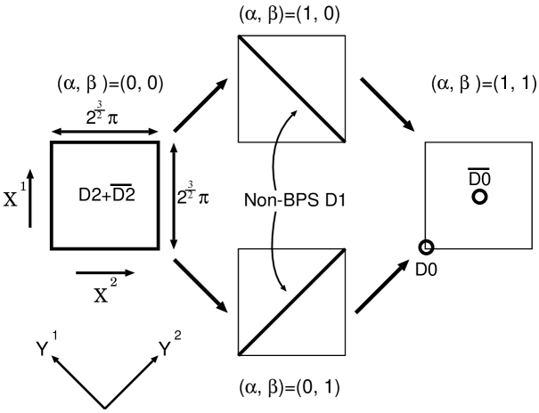
Figure 4.2: The tachyon condensation in $D2+\overline{D2}$ system

4.4 Calculation of the Vacuum Amplitude

In this section we will calculate the vacuum amplitude of a $D2+\overline{D2}$ system for every value of parameters $\alpha$ and $\beta$ and read off the open string spectrum [47, 46]. As a result it will be shown that the additional operator in eq.(4.3.36) is indeed required in order to satisfy Cardy’s condition [54].

First note that in the new coordinate system $(\phi^{i},\eta^{i}_{L},\eta^{i}_{R})$ the Virasoro generator $L_{0}$ of closed strings is given by

$$L_{0}=\frac{1}{2}\phi^{i}_{0}\phi_{i0}+\sum^{\infty}_{m=1}\phi^{i}_{-m}\phi_{im}+\sum^{\infty}_{r\in{\bf Z}+\nu}r\eta^{i}_{-r}\eta_{ir}+a+\cdots\cdots,$$ (4.4.43)

where $a$ is the zero point energy which is equal to $-1/2~{}(0)$ for NS (R)-sector, and $\cdots$ part denotes the contribution from directions other than $x^{1}$ and $x^{2}$. $\tilde{L}_{0}$ can be obtained by adding the tilde over all oscillators. We can easily obtain this expression if we notice that the explicit form of energy momentum tensor is preserved under bosonization (4.2). By using these expressions in the closed string propagator (2.1.36) we can calculate the vacuum amplitude $Z(\alpha,\beta)=\langle B(\alpha,\beta)|\Delta|B(\alpha,\beta)\rangle$, which is given by

$$Z_{NSNS}(\alpha,\beta) \equiv \langle B(\alpha,\beta)|\Delta|B(\alpha,\beta)\rangle_{\scriptscriptstyle NSNS}$$

$$= \frac{(T_{2})^{2}V_{3}}{2}\int^{\infty}_{0}ds(4\pi s)^{-\frac{7}{2}}\Biggl{[}\sum_{(w_{\phi}^{1},w_{\phi}^{2})\in{\bf Z}^{2}}\Bigl{\{}\cos^{2}(\pi\alpha w_{\phi}^{1})\cos^{2}(\pi\beta w_{\phi}^{2})$$

$$\ +\sin^{2}(\pi\alpha w_{\phi}^{1})\sin^{2}(\pi\beta w_{\phi}^{2})\Bigr{\}}q^{(w_{\phi}^{1})^{2}+(w_{\phi}^{2})^{2}}\frac{f_{3}(q)^{8}}{f_{1}(q)^{8}}-2\frac{f_{4}(q)^{6}f_{3}(q)^{2}}{f_{1}(q)^{6}f_{2}(q)^{2}}\Biggl{]},$$

$$Z_{RR}(\alpha,\beta) \equiv \langle B(\alpha,\beta)|\Delta|B(\alpha,\beta)\rangle_{\scriptscriptstyle RR}$$ (4.4.44)

$$= -\frac{(T_{2})^{2}V_{3}}{2}\int^{\infty}_{0}ds(4\pi s)^{-\frac{7}{2}}\Biggl{[}\sum_{(w_{\phi}^{1},w_{\phi}^{2})\in{\bf Z}^{2}}\Biggl{\{}\cos^{2}\left(\pi\alpha\left(w_{\phi}^{1}+\frac{1}{2}\right)\right)\cos^{2}\left(\pi\beta\left(w_{\phi}^{2}+\frac{1}{2}\right)\right)$$

$$\!\!+\sin^{2}\left(\pi\alpha\left(w_{\phi}^{1}+\frac{1}{2}\right)\right)\sin^{2}\left(\pi\beta\left(w_{\phi}^{2}+\frac{1}{2}\right)\right)\Biggr{\}}q^{(w_{\phi}^{1}+\frac{1}{2})^{2}+(w_{\phi}^{2}+\frac{1}{2})^{2}}\frac{f_{2}(q)^{8}}{f_{1}(q)^{8}}\Biggl{]},$$

where $q=e^{-s}$, and $V_{3}$ is the volume of a D2-brane. $f_{i}(q)~{}(i=1,2,3,4)$ are the modular functions defined in eq.(2.1).

Let us transform this expression into the form of one-loop amplitude of open strings like eq.(2.1.41). By defining $t$ by $t=\frac{\pi}{s}$ and using the modular properties (2.1) of the modular functions $f_{i}(q)$, we can obtain the following open string amplitude:

$$Z^{open}_{NS}(\alpha,\beta) = 2^{-2}\pi^{-1}V\int^{\infty}_{0}dt\ t^{-\frac{3}{2}}\sum_{(n_{1},n_{2})\in{\bf Z}^{2}}\Biggl{[}\frac{1}{2}(\tilde{q}^{n_{1}^{2}+n_{2}^{2}}+\tilde{q}^{(n_{1}-\alpha)^{2}+(n_{2}-\beta)^{2})})\frac{f_{3}(\tilde{q})^{8}}{f_{1}(\tilde{q})^{8}}$$

$$~{}~{}~{}~{}~{}~{}~{}~{}~{}~{}~{}~{}~{}~{}~{}~{}~{}~{}~{}~{}-\frac{1}{2}(-1)^{n_{1}+n_{2}}(\tilde{q}^{n_{1}^{2}+n_{2}^{2}}+\tilde{q}^{(n_{1}-\alpha)^{2}+(n_{2}-\beta)^{2}})\frac{f_{4}(\tilde{q})^{8}}{f_{1}(\tilde{q})^{8}}\Biggl{]},$$

$$Z^{open}_{R}(\alpha,\beta) = -2^{-2}\pi^{-1}V\int^{\infty}_{0}dt\ t^{-\frac{3}{2}}\sum_{(n_{1},n_{2})\in{\bf Z}^{2}}\tilde{q}^{n_{1}^{2}+n_{2}^{2}}\frac{f_{2}(\tilde{q})^{8}}{f_{1}(\tilde{q})^{8}},$$ (4.4.45)

where $\tilde{q}=e^{-\pi t}$ and $V\left(\equiv\frac{V_{3}}{(2\sqrt{2}\pi)^{2}}\right)$ is the “volume” of the time direction. Here we have used the following identities of $f_{i}(q)$:

$$\sum_{n}q^{n^{2}}=f_{1}(q)f_{3}(q)^{2} \sum_{n}(-1)^{n}q^{n^{2}}=f_{1}(q)f_{4}(q)^{2},$$ ,

$$\sum_{n}q^{(n-\frac{1}{2})^{2}}=f_{1}(q)f_{2}(q)^{2} f_{2}(q)f_{3}(q)f_{4}(q)=\sqrt{2}\ .$$ , (4.4.46)

Now it is obvious that for each value of $\alpha$ and $\beta$ the open string spectrum is well-defined only if we consider the additional operator (4.3.36) defined in the previous section. If we did not include the operator (4.3.36) in the boundary state $|B(\alpha,\beta)\rangle_{\scriptscriptstyle NSNS(RR)}$, the number of open string states for given $n_{1},n_{2}$ would be fractional. This physically important constraint is also called Cardy’s condition [54].

Finally let us see what kind of open string amplitudes appears at particular values of $\alpha$ and $\beta$. In the case of $(\alpha,\beta)=(1,0)$ or $(0,1)$ we obtain the following amplitude [47, 46]

$$Z(1,0)=Z(0,1) = 2^{-2}\pi^{-1}V\int^{\infty}_{0}dt\ t^{-\frac{3}{2}}\sum_{(n_{1},n_{2})\in{\bf Z}^{2}}\tilde{q}^{n_{1}^{2}+n_{2}^{2}}\frac{f_{3}(\tilde{q})^{8}-f_{2}(\tilde{q})^{8}}{f_{1}(\tilde{q})^{8}},$$ (4.4.47)

$$= 4\pi V\int^{\infty}_{0}\frac{dt}{2t}{\rm Tr}_{\scriptscriptstyle NS-R}\tilde{q}^{2L_{0}}.$$

Therefore we can identify the system as a non-BPS D1-brane whose length is $4\pi$ as we expected in figure 4.2 (compare the above amplitude with eq.(2.3.66)). The other case left is $(\alpha,\beta)=(1,1)$ and its amplitude can be written as [47]

$$Z(1,1) = 2^{-2}\pi^{-1}V\int^{\infty}_{0}dt\ t^{-\frac{3}{2}}\sum_{(n_{1},n_{2})\in{\bf Z}^{2}}\Biggl{[}\tilde{q}^{n_{1}^{2}+n_{2}^{2}}\frac{f_{3}(\tilde{q})^{8}-f_{2}(\tilde{q})^{8}}{f_{1}(\tilde{q})^{8}}-(-1)^{n_{1}+n_{2}}\tilde{q}^{n_{1}^{2}+n_{2}^{2}}\frac{f_{4}(\tilde{q})^{8}}{f_{1}(\tilde{q})^{8}}\Biggl{]},$$

$$= 2V\int^{\infty}_{0}\frac{dt}{t}\frac{1}{\sqrt{16\pi^{2}t}}\sum_{(m_{1},m_{2})\in{\bf Z}^{2}}\Biggl{[}\tilde{q}^{2m_{1}^{2}+2m_{2}^{2}}\frac{f_{3}(\tilde{q})^{8}-f_{4}(\tilde{q})^{8}-f_{2}(\tilde{q})^{8}}{2f_{1}(\tilde{q})^{8}}$$

$$~{}~{}~{}~{}~{}~{}~{}~{}~{}~{}~{}~{}~{}~{}~{}~{}~{}~{}~{}~{}~{}~{}~{}~{}~{}~{}~{}~{}~{}~{}~{}~{}~{}~{}~{}~{}~{}+\tilde{q}^{2(m_{1}+\frac{1}{2})^{2}+2(m_{2}+\frac{1}{2})^{2}}\frac{f_{3}(\tilde{q})^{8}+f_{4}(\tilde{q})^{8}-f_{2}(\tilde{q})^{8}}{2f_{1}(\tilde{q})^{8}}\Biggl{]},$$

$$= 2V\int^{\infty}_{0}\frac{dt}{2t}{\rm Tr}_{NS-R}\left[\frac{1+(-1)^{F}}{2}\tilde{q}^{2L_{0}}\right]+2V\int^{\infty}_{0}\frac{dt}{2t}{\rm Tr}_{NS-R}\left[\frac{1-(-1)^{F}}{2}\tilde{q}^{2L_{0}}\right],$$

where we have defined $m_{1}=\frac{n_{1}+n_{2}}{2},m_{2}=\frac{n_{1}-n_{2}}{2}$. Note that this partition function counts not only the degrees of freedom of open strings stretching between a brane and an antibrane but also those of open strings both of whose end points are on the same D-branes. This explicitly shows that the system is equivalent to a D0-brane and an anti D0-brane. Moreover, from the half-integer power of $\tilde{q}$ in the second term of the second line we can see that these two D-branes are separated from each other by $\Delta x_{1}=\Delta x_{2}=\sqrt{2}\pi$. This is consistent with figure 4.2.

4.5 Tachyon Condensation at General Radii of Torus

In the previous sections we have proved the tachyon condensation by the conformally invariant method called marginal deformation. In this proof the crucial ingredient was to fix the radius of the torus $T^{2}$ at some convenient value in order to keep the conformal invariance. However, its physical situation is too special and it is desirable to generalize the argument of tachyon condensation into arbitrary radii of the torus [39, 42, 47].

Before its analysis let us consider what happens in the internal region of the parameter space $(\alpha,\beta)$. In the previous section we have considered only edge points $((\alpha,\beta)=(0,0),~{}(1,0),~{}(0,1),~{}(1,1))$ of this parameter space. This is because the boundary state $|B(\alpha,\beta)\rangle$ except those edge points does not correspond to any physical objects we know. This fact becomes obvious if we consider general radii of the torus $T^{2}$. At general radii the process of tachyon condensation is an off-shell phenomenon and generates tachyon potential as we explained in section 4.1. In tachyon potential physical objects we already know appear at its extremum points because these points satisfy the equation of motion of open strings ($\alpha^{\prime}$ corrected Yang-Mills-Higgs equation) and preserve the conformal invariance.

Here what we would like to show is that if we consider general radii of the torus $T^{2}$ the conformal invariance is only kept at edge points of the parameter space $(\alpha,\beta)$. Its proof is as follows. First the tachyon potential can be regarded as the total energy (mass) of the D-brane system we are considering, and the form of potential at the special radii $(R_{1}=R_{2}=\sqrt{2})$ can be calculated by the internal product $V_{R_{i}}(\alpha,\beta)=\langle 0|B(\alpha,\beta)\rangle_{\scriptscriptstyle NSNS}$, where $\alpha$ and $\beta$ denote the expectation values of the tachyons $T_{1}$ and $T_{2}$ in eq.(4.2.8). Indeed as we can see in eq.(3.2.58) and appendix B this quantity is proportional to the disk partition function, and it is consistent with boundary string field theory. Moreover by using equation (4.3.38) we can see $V_{R_{i}}(\alpha,\beta)=T_{2}=$ constant. This fact just indicates that the tachyon potential is flat and we can use the marginal deformation as we explained in section 4.1. Next, we consider the deformed potential $V_{R_{i}+\Delta R_{i}}(\alpha,\beta)$ by $R_{i}\rightarrow R_{i}+\Delta R_{i}~{}~{}(i=1,2)$. As we have explained in the last paragraph the potential ceases to be flat at general radii and this deformed potential gets nontrivial dependence of $\alpha$ and $\beta$. Here instead of using string field theory we will use a simple trick. We consider the infinitesimal deformation of this potential, which is given by

$$V_{R_{i}+\Delta R_{i}}(\alpha,\beta)\cong V_{R_{i}}(\alpha,\beta)+\sum_{i}\Delta R_{i}\frac{d}{dR_{i}}V_{R_{i}}(\alpha,\beta)$$

$$=T_{2}+\sum_{i}\Delta R_{i}\times\langle 0|\psi_{L}^{i}(0)\psi_{R}^{i}(0)|B(\alpha,\beta)\rangle_{\scriptscriptstyle NSNS}.$$ (4.5.49)

Here $\psi_{L}^{i}(0)\psi_{R}^{i}(0)$ is a vertex operator with $(-1,-1)$ picture, which represents the radius deformation. Therefore, to find extremum points of the radius deformed tachyon potential we have to solve the following equations

$$\frac{\partial}{\partial\alpha}\langle 0|\psi^{i}_{L}(0)\psi^{i}_{R}(0)|B(\alpha,\beta)\rangle_{\scriptscriptstyle NSNS}=\frac{\partial}{\partial\beta}\langle 0|\psi^{i}_{L}(0)\psi^{i}_{R}(0)|B(\alpha,\beta)\rangle_{\scriptscriptstyle NSNS}=0.$$ (4.5.52)

Calculating this by bosonizing $\psi^{i}_{L}$ and $\psi^{i}_{R}$ we can obtain equations $\sin(\pi\alpha)=\sin(\pi\beta)=0$ and the solution is $(\alpha,\beta)=(0,0),~{}(0,1),~{}(1,0)$ and $(1,1)$, which we have just investigated.

As the next step let us compare the total mass between $D2+\overline{D2}$, non-BPS $D1$ and $D0+\overline{D0}$ at general radii $(R_{1},~{}R_{2})$ of the torus. These values become as follows

$$\begin{array}[]{cl}2T_{2}(2\pi R_{1})(2\pi R_{2}){}{}&~{}~{}(\mbox{for}~{}~{}D2+\overline{D2}),\\ \sqrt{2}T_{1}(2\pi\sqrt{R_{1}^{2}+R_{2}^{2}}){}{}&~{}~{}(\mbox{for non-BPS}~{}D1),\\ 2T_{0}{}{}&~{}~{}(\mbox{for}~{}~{}D0+\overline{D0}),\end{array}$$ (4.5.53)

where we have assumed that a non-BPS D1-brane winds along the diagonal line of the torus like figure 4.2. Note that the tension of a non-BPS D1-brane is $\sqrt{2}$ times as large as that of a BPS D1-brane (see equation (2.3.65)). If we write the masses of these D-brane systems as $M_{D2+\overline{D2}},~{}M_{ND1}$ and $M_{D0+\overline{D0}}$, we can obtain the following relations

$$\begin{array}[]{cl}M_{D0+\overline{D0}}\leq M_{ND1}\leq M_{D2+\overline{D2}}{}{}&~{}~{}(\mbox{when}~{}\frac{1}{R_{1}^{2}}+\frac{1}{R_{2}^{2}}\leq 1),\\ &\\ M_{D0+\overline{D0}}\leq M_{D2+\overline{D2}}\leq M_{ND1}{}{}&~{}~{}(\mbox{when}~{}\frac{1}{R_{1}^{2}}+\frac{1}{R_{2}^{2}}\geq 1~{}~{}\mbox{and}~{}~{}R_{1}R_{2}\geq 2),\\ &\\ M_{D2+\overline{D2}}\leq M_{D0+\overline{D0}}\leq M_{ND1}{}{}&~{}~{}(\mbox{when}~{}R_{1}R_{2}\leq 2~{}~{}\mbox{and}~{}~{}R_{1}^{2}+R_{2}^{2}\geq 4),\\ &\\ M_{D2+\overline{D2}}\leq M_{ND1}\leq M_{D0+\overline{D0}}{}{}&~{}~{}(\mbox{when}~{}R_{1}^{2}+R_{2}^{2}\leq 4).\end{array}$$ (4.5.54)

Furthermore, the condition that there are no tachyons on a $D2+\overline{D2}$ system can be seen in eq.(4.1.7) as

$$\frac{1}{R_{1}^{2}}+\frac{1}{R_{2}^{2}}\geq 1.$$ (4.5.55)

In the same way we can examine the condition of the absence of tachyons on a $D0+\overline{D0}$ system and it is given by

$$R_{1}^{2}+R_{2}^{2}\geq 4,$$ (4.5.56)

which means that a D$0$-brane is separated enough from an anti D$0$-brane (see figure 4.2). Here one interesting thing is that the equations which determine whether a tachyon exists are the same as some equations in eq.(4.5.54). Note that there always exists a tachyonic mode on the non-BPS D1-brane.

From all of the above results ((4.5.54) $\sim$ (4.5.56)) we can understand what the stablest object is among them (see figure 4.3). If $R_{1}$ and $R_{2}$ are very large, the mass of D2-branes is heavier than that of D0-branes and a $D2+\overline{D2}$ system decays to a $D0+\overline{D0}$ system. On the contrary, if $R_{1}$ and $R_{2}$ are very small, the opposite process happens. Indeed in the region over line (a) in figure 4.3 a tachyonic mode appears on a $D2+\overline{D2}$ system and this is consistent with the fact that D2-branes are heavier than D0-branes. This kind of fact also holds in the region under line (b).

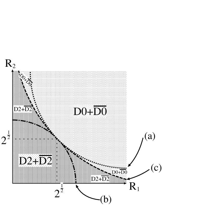
Figure 4.3: The phase diagram about the stability of D-brane systems. If the torus is large a $D0+\overline{D0}$ system is stabler, and if the torus is small a $D2+\overline{D2}$ system is. The equations of three curves in the phase diagram are given by $(a)~{}\frac{1}{R_{1}^{2}}+\frac{1}{R_{2}^{2}}=1,~{}~{}~{}(b)~{}R_{1}^{2}+R_{2}^{2}=4,~{}~{}~{}(c)~{}R_{1}R_{2}=2$.

The point with $R_{1}=R_{2}=\sqrt{2}$ is the only one where all kinds of D-brane systems have exactly the same mass and some tachyonic mode on them becomes massless. Therefore, only at this point we can use the method of the marginal deformation, while in the other regions the conformal invariance is broken and the process of tachyon condensation is an off-shell one. For example, at the point $R_{1}=2,~{}R_{2}=\frac{2\sqrt{3}}{3}$ the lowest mode on a $D2+\overline{D2}$ system becomes massless (see equation (4.1.7)) and it looks like we can use the marginal deformation. However, at this point the operator (4.2.15) is not a truly marginal operator and switching on this operator causes a renormalization group flow.

The most subtle region in figure 4.3 is one which is surrounded between line (a) and (b). In this region any tachyonic modes do not exist on either $D2+\overline{D2}$ or $D0+\overline{D0}$. This fact indicates that both of the systems are perturbatively stable. On the other hand line (c) determines which system is heavier, thus we expect that the stabler object is determined by its mass. In other words the heavier D-brane system is metastable and nonperturbatively decays to the lighter one by the quantum mechanical tunneling effect.

Note that the argument of comparison of masses among various objects here is not an exact result because the masses of unstable systems obtain the quantum corrections as we have seen in eq.(2.3.64). In this sense figure 4.3 is correct only in the weak coupling string theory.

Chapter 5 Conclusion and Future Problems

5.1 Conclusion

In this thesis we have considered the tachyon condensation on unstable D-brane systems in the flat space. Although various methods are known to analyze the tachyon condensation, in this thesis we have dealt with the boundary string field theory and the marginal deformation.

The string field theory is a general method to analyze off-shell phenomena in string theory. Especially the boundary string field theory enables us to describe the tachyon condensation in the exact manner. Although we start with the Batalin-Vilkovisky formulation to construct it, this theory can simply be regarded as a natural extension of the sigma model calculation of the disk partition function.

This theory also determines the action of its effective field theory for non-BPS systems. In superstring theory the action consists of two parts. One is the Dirac-Born-Infeld action and the other is the Wess-Zumino term (RR-coupling). If we assume some approximation scheme, we can write down the explicit form of the Dirac-Born-Infeld type action. Moreover we have found that the Wess-Zumino terms on brane-antibrane systems and non-BPS D-branes can exactly be written by the superconnections, which were known in the mathematics. These results are consistent with K-theory arguments and the tachyon condensation.

On the other hand in the special situation we can describe the tachyon condensation in the conformally invariant manner. In this thesis we have used the boundary state formalism to describe it. The boundary state formalism is convenient to examine the interaction between D-branes and closed strings, thus we were able to see how RR-charges of D-branes with lower dimension appear during the tachyon condensation. Moreover by changing radii of a torus we could understand the phase diagram about stability of various non-BPS systems.

5.2 Problems in Boundary String Field Theory

We think that the analyses in this thesis have given enough evidence to show various aspects of tachyon condensation. However, we have several problems which have not been solved. The first problem is about the relation between the cubic string field theory [15] (or Berkovits’ supersymmetrized version [17]) and the boundary string field theory [22]. Although the appearance of these two theories is quite different, there should be some relationship between two as long as they describe the same physics. The naive expectation is that they are related to each other by a redefinition of target space fields. However, we do not know its explicit form.

The next problem is how we should solve the nonrenormalizability of boundary string field theory. The calculations we did in chapter 3 were restricted to those with only renormalizable terms included in the boundary part of the sigma model. One of principles of boundary string field theory is to include all possible terms in the boundary action, while we do not know how to calculate it. In this sense the cases where we can use boundary string theory are rather limited to special situations than cubic string field theory.

The third problem is related to the second one. We have not yet understood why boundary string field theory gives exact answers to problems of tachyon condensation even though we do not include massive terms in the boundary action [26, 28]. As we saw in section 3.8 the point is whether all the one-point functions $\frac{\partial S}{\partial\lambda^{i}}|_{\lambda^{i}=0}$ of massive fields $\lambda^{i}$ become zero or not. If this is true we can admit that we have calculated the truly exact quantities, however we can not verify it. Anyway the reason why we could obtain the desirable results might be related to the integrability of path integrals. In other words this might be because the renormalization group is closed in the algebraic sense. For example the RG flow does not induce any divergences in coefficients of nonrenormalizable terms if we only include renormalizable terms. In this case the theory is well-defined and we might be able to regard its answer as an exact one.

The fourth problem is about the quantum theory of boundary string field theory. We do not know how to consistently incorporate quantum corrections in the sense of target space and how to apply it to tachyon condensation. The first naive approach is to regard the one-loop correction to the action $S$ of string field theory as a cylinder amplitude with non-conformal worldsheet action $I_{B}$. However, there are not any dualities which connect the cylinder with the annulus because the conformal invariance is broken [69, 109]. For example, if we consider the general boundary state in eq.(2.2.54) with an off-shell boundary action $I_{B}$, we can not assert that the interaction amplitude between two D-branes can be re-expressed as some kind of open string amplitude. Moreover, there is not any support to this idea like the BV-formalism of classical boundary string field theory.

Finally we have a question about the relation between the worldsheet SUSY and the target space SUSY. In boundary string field theory we have imposed the worldsheet SUSY in the boundary actions for a brane-antibrane system and a non-BPS D-brane. Although there do not exist any principles to impose the worldsheet SUSY, this description was successful as we saw in chapter 3 even without the target space supersymmetry. It is mysterious.

5.3 General Problems in the Tachyon Condensation

The first general question is how to include target space fermions in the action $S$ of string field theory. In boundary string field theory only bosonic target space fields appear in the boundary sigma model in RNS formalism. There is also this problem in Berkovits’ string field theory [17]. Of course we can include them by constructing spin-fields from RNS variables, but this is not applicable to off-shell phenomena like tachyon condensation. A naive resolution to this problem is to use Green-Schwarz formalism [65] or pure-spinor formalism [66] instead of RNS formalism. However, we have not yet understood how to include the GSO-odd sector like a tachyon in the sigma model action, and we do not know what kind of principles determines the explicit form of boundary action $I_{B}$. Indeed we can find that the insertion of the boundary fermions $\eta$ and $\bar{\eta}$ which appeared in eq.(3.3.68) can not be used in these formulations.

The next problem is to extend the analysis in the flat space into that in the curved space. The non-BPS systems and their dynamical phenomena in the curved space are also interesting. Although in general these are difficult to analyze, the orbifold is one of simple curved backgrounds which we can deal with by using the conformal field theory technique. Indeed we can argue the tachyon condensation by the on-shell description in the orbifold $T^{4}/{\bf Z}_{2}$ [47, 43, 44, 48, 38, 110]. The concrete calculation by using the boundary state is almost the same as that in the flat space, except the subtlety coming from appearance of the twisted sector in the boundary state [47]. The physical difference appears in the fact that some non-BPS D1-branes become stable if we choose appropriate radii of the torus $T^{4}$, although they are always unstable in the flat space. We can prove this fact by examining its open string spectrum. Indeed modes with negative mass square are dropped by the orbifold projection which is inserted in the open string partition function. Moreover the non-BPS D1-brane can be interpreted as a BPS D2-brane wound on a nonsupersymmetric cycle of $T^{4}/{\bf Z}_{2}$ [37, 38, 40]. Maybe this can be generalized into the argument in general K3 surfaces if we regard $T^{4}/{\bf Z}_{2}$ as the orbifold limit of it.

How about the string field theory? Of course the analyses in curved space is difficult in both of the cubic string field theory (or Berkovits’ supersymmetrized version) and the boundary string field theory except a few backgrounds like orbifolds [111, 112]. However, there is a theorem which states that the explicit form of tachyon potential does not depend on which closed string background we choose. This is called the universality of the tachyon potential [74]. What we need to do or would like to do is to find other universal properties. As we said in chapter 3, the original name of boundary string field theory was “the background independent open string field theory” [22] because bulk action (3.1.1) is background independent. Thus, the boundary string field theory might be suitable to seek for the universality of the tachyon condensation.

The third problem is about the relation between the time of the target space and the worldsheet renormalization scale. As we can see in the boundary string field theory, when unstable D-brane systems decay there seems to be a correspondence between the flow of the time in the target space and the one-dimensional RG-flow in the worldsheet. Therefore, it might be important to consider time dependent backgrounds in string theory.

The fourth problem is how we can understand nonperturbative instability of non-BPS systems. Until now any nonperturbative corrections of string field theory have not been known. It might be captured as some nonperturvative corrections in the worldvolume field theory on D-branes[113].

5.4 Closed String Dynamics

A problem occurs when we pay attention to the vacuum without D-branes which appears after tachyon condensation on unstable D-brane systems. In boundary string field theory the stable vacuum appears at the point $|T|\rightarrow\infty$ and the total action like eq.(3.6.7) vanishes there. This seems consistent with the fact that there are no open string degrees of freedom. On the other hand, if we expand the action around $|T|=\infty$, some unknown fluctuation modes can appear. Indeed if we take the limit $|T|\rightarrow\infty$ after we move to the Hamiltonian formalism, the Hamiltonian remains nonzero [92]. This indicates that some unknown stuff is left at the stable vacuum. The recent idea to solve it is to consider them as closed strings. In other words, closed strings appear as bound states of classical open strings [93, 91, 92, 90, 88]. For the time being it is difficult to construct a closed string from open strings in the level of the classical string field theory or its classical effective field theory. Anyway even if closed strings do not appear as bound states of classical open strings, we already know that they appear as intermediate states in one-loop open string diagrams. In this sense we can say that the open string field theory includes closed strings in the quantum level, and we can expect that open string field theory already knows the closed string theory [114, 115]. The open string field theory might be regarded as a nonperturbative definition of the total string theory in the same way as the matrix model [3].

Anyway we would like to consider the closed string dynamics as a next step. Indeed if we put some non-BPS systems in the flat space, the D-branes themselves bend the space because of their masses. This is called the back reaction of these D-branes, while such a closed string effect comes from the quantum level of open string field theory. If we understand the open string tachyon dynamics in the quantum level we might be able to use it as a model of evaporation of a blackhole or the cosmological evolution. As we said in chapter 3, the decay of non-BPS systems in the context of classical open string field theory has correspondence to the one-dimensional renormalization group flow in the worldsheet. In the same way we might relate the worldsheet renormalization group flow with the complete description of decay of these D-branes accompanying the radiation of closed strings. Moreover there might exist the dynamical version of holography and we might find some correspondence between the open string theory and closed string theory.

This problem will be related to that of the closed string tachyon condensation in the theory with a closed string tachyon like type 0 theory. We have not yet understood the relation between the two-dimensional RG-flow and the dynamics of the target space, which are expected to be decay of the spacetime. Although the idea of this relation was inspired by the open string tachyon condensation which has been successful, this expectation might not always be applied to the closed string side:

The first reason is that we do not know whether there is a global minimum in the tachyon potential of closed strings. Sen’s conjecture of open string tachyon condensation [6] was based on it, from which we can say that a theory with a tachyon is not inconsistent but only stays in a dynamical phase. Although that was correct in the open string theory, we do not know whether it is correct in the closed string theory also.

The second reason comes from the fact that the off-shell target space theory of closed strings (closed string field theory) might not be well-defined. The closed string theory represents the gravitation, which is not a usual field theory like gauge theories. Thus we might not be able to apply a naive field theoretical idea to gravitational theories like the closed string theory. For example we can imagine that the expectation value of the dilaton changes during off-shell gravitational phenomena, and this means that the string coupling is not a constant during those processes. In this case we might not be able to rely on the fundamental assumption that systems are described by a classical quantity plus its quantum correction. In other words we might have to start with a unknown nonperturbative quantity, and we might not be able to take the classical limit in off-shell gravitational phenomena. If that is the case the closed string field theory might become meaningless.

The third reason is how we can define the quantity which decreases along the two-dimensional renormalization group flow. In open string theory this quantity is given by the g-function or the action of string field theory. In the target space we can interpret this as energy or mass of D-branes. On the other hand the c-function is known which decreases along the two-dimensional renormalization group flow corresponding to the g-function. This is equal to the central charge at conformal fixed points. The problem is that theories at IR fixed points become non-critical string theories since the values of the c-function at IR-fixed points are always smaller than those at UV fixed points. As long as we have not understood whether we can regard non-critical string theories as physically meaningful ones, we can not conclude that this idea is correct.

Moreover, even if we can accept this idea the difficult problem is how to define the notion of energy in the target space of closed string theory corresponding to the c-function in the worldsheet. In fact it is known that we can not define the universal notion of energy in the general relativity except a few backgrounds like ADM energy in the asymptotically flat background. Therefore, even if we would like to consider the closed string tachyon condensation, we can not define the energy in the universal way and it crucially depends on which background we choose [116, 117, 118]. In this way this problem comes from the fact that we have not understood the background independence of string theory. This is a difficult and important problem.

One possible idea to avoid considering the problem of closed string tachyon condensation is to restrict consistent closed string backgrounds to on-shell ones. This idea comes from the holography [119] in AdS/CFT correspondence [4]. According to the holography, a non-local d-dimensional gravitational theory, which is difficult to deal with, has some correspondence with a (d-1)-dimensional field theory, which we know a lot. In this way we can interpret the closed string dynamics by using field theories. However, the holography is mysterious in the sense that we do not know where it comes from.

Anyway the serious problems of the closed string dynamics stem from the fact that we have not yet understood the two important notions-“the backreation” and “the background independence”. To fully solve these problems we might need to go beyond the perturbative string theory. Until now the string theory has been developed by using similar ideas which come from field theories, like supersymmetry or duality or soliton etc. However, we have come to the stage where we have to find physically new ideas which can not be seen in field theories. In this sense the holography might be one of important ingredients to go beyond old ideas and to understand the nonperturbative formulation of string theory or quantum gravity.

Acknowledgements

     I would like to thank Prof. Kazuo Fujikawa for a lot of advice and continuous encouragement. I am also grateful to Dr. Seiji Terashima, Dr. Michihiro Naka and Dr. Tadashi Takayanagi for fruitful collaborations and many useful discussions. Without them I could not have finished writing this manuscript. I am thankful to all the staffs and students in the high energy physics theory group of University of Tokyo for giving me the opportunity to study a lot of things and having discussions.

The work of the author was supported by JSPS Research Fellowships for Young Scientists.

Appendix A Conventions

A.1 Conformal Field Theory in the Flat Space Background

In this section we fix the convention about the conformal field theory in the flat space background. In this thesis we set $\alpha^{\prime}$ to $2$, and the convention is almost identical to that of [99]. The sigma model action in the flat space is given by

$$I_{0}=\frac{1}{4\pi}\int d^{2}z(\partial X^{\mu}\bar{\partial}X_{\mu}-i\psi^{\mu}_{L}\bar{\partial}\psi_{L\mu}+i\psi^{\mu}_{R}\partial\psi_{R\mu}).$$ (A.1.1)

Here we have already fixed the worldsheet gauge freedom by taking the conformal gauge, while we have omitted the terms with the ghosts $(b,c~{};~{}\beta,\gamma)$ because in this thesis we can mostly do without considering the ghost contribution.

Operator product expansions (OPE)

     From this action we can obtain the operator product expansions (OPE) for the fields $(X^{\mu}(z,\bar{z}),~{}\psi^{\mu}_{L}(z),~{}\psi^{\mu}_{R}(\bar{z}))$

$$X^{\mu}(z)X^{\nu}(0) \sim -\delta^{\mu\nu}{\mbox{ln}}|z|^{2},$$

$$\psi^{\mu}_{L}(z)\psi^{\nu}_{L}(0) \sim \delta^{\mu\nu}\frac{i}{z}~{},~{}\psi^{\mu}_{R}(\bar{z})\psi^{\nu}_{R}(0)\sim-\delta^{\mu\nu}\frac{i}{\bar{z}}.$$ (A.1.2)

Here we have defined $z=e^{-\sigma_{2}+i\sigma_{1}}$ as the radial plane coordinate of the world sheet and $w=\sigma_{1}+i\sigma_{2}$ as its cylindrical coordinate. Thus, $\sigma_{1}$ and $\sigma_{2}$ represent the worldsheet coordinates of space and time, respectively.



Mode expansions for closed strings

     Next let us list the closed string mode expansions of fields $(X^{\mu},~{}\psi^{\mu}_{L},~{}\psi^{\mu}_{R})$:

$$X^{\mu}_{L}(z)=x^{\mu}_{L}-i\alpha^{\mu}_{0}\ln z+i\sum_{m\neq 0}\frac{\alpha^{\mu}_{m}}{mz^{m}},$$

$$X^{\mu}_{R}(\bar{z})=x^{\mu}_{R}-i\tilde{\alpha}^{\mu}_{0}\ln\bar{z}+i\sum_{m\neq 0}\frac{\tilde{\alpha}^{\mu}_{m}}{m\bar{z}^{m}},$$

$$\psi^{\mu}_{L}(z)=i^{\frac{1}{2}}\sum_{r\in Z+\nu}\frac{\psi^{\mu}_{r}}{z^{r+\frac{1}{2}}}~{},~{}\psi^{\mu}_{R}(\bar{z})=i^{-\frac{1}{2}}\sum_{r\in Z+\nu}\frac{\tilde{\psi}^{\mu}_{r}}{\bar{z}^{r+\frac{1}{2}}},$$ (A.1.3)

where $X^{\mu}(z,\bar{z})=X^{\mu}_{L}(z)+X^{\mu}_{R}(\bar{z})~{},~{}p^{\mu}_{L}=\alpha^{\mu}_{0}~{},~{}p^{\mu}_{R}=\tilde{\alpha}^{\mu}_{0}$, and $\nu=\frac{1}{2}$ represents NS-sector and $\nu=0$ R-sector. The Virasoro generators $L_{0}$ and $\tilde{L}_{0}$ can be written as

$$L_{0}=\frac{1}{2}\alpha^{\mu}_{0}\alpha_{\mu 0}+\sum^{\infty}_{m=1}\alpha^{\mu}_{-m}\alpha_{\mu m}+\sum^{\infty}_{r\in{\bf Z}+\nu}r\psi^{\mu}_{-r}\psi_{\mu r}+a,$$ (A.1.4)

where $a$ is the zero point energy which is equal to $-1/2~{}(0)$ for NS (R)-sector, and $\tilde{L}_{0}$ can be obtained by replacing $\alpha^{\mu}_{m},~{}\psi^{\mu}_{r}$ with $\tilde{\alpha}^{\mu}_{m},~{}\tilde{\psi}^{\mu}_{r}$, respectively.

The subtle point is about the zero modes $(x^{\mu}_{L},p_{L}^{\mu}~{};~{}x^{\mu}_{R},p_{R}^{\mu})$ of the bosonic fields $X^{\mu}(z,\bar{z})$. If we consider a noncompactified direction, the valuable $x^{\mu}$ defined by $x^{\mu}\equiv x^{\mu}_{L}+x^{\mu}_{R}$ represents the physical coordinate and the physical momentum $p^{\mu}$ is defined by $p^{\mu}=p^{\mu}_{L}=p^{\mu}_{R}$. By the canocial quantization these valuables have the usual quantization condition

$$[x^{\mu},p^{\nu}]=i\eta^{\mu\nu},$$ (A.1.5)

where $\eta^{\mu\nu}=\mbox{diag}(-1,+1,+1,\cdots)$.

On the other hand if we consider a compactified direction on $S^{1}$ with radius $R_{\mu}$, the crucial difference appears in the the momentum modes $p^{\mu}_{L}$ and $p^{\mu}_{R}$ which are defined by

$$p^{\mu}_{L}~{}\equiv~{}\frac{n^{\mu}}{R_{\mu}}+\frac{w^{\mu}R_{\mu}}{2},$$

$$p^{\mu}_{R}~{}\equiv~{}\frac{n^{\mu}}{R_{\mu}}-\frac{w^{\mu}R_{\mu}}{2},$$ (A.1.6)

where $n^{\mu}$ and $w^{\mu}~{}$ are integer numbers which represent the discrete momentum and the winding number in that direction, respectively.

The nonzero modes can be treated irrespective of whether we consider a compactified direction or a noncompactified direction. The OPE relations (A.1) are equivalent to the following (anti)commutation relations for modes :

$$[\alpha^{\mu}_{m},\alpha^{\nu}_{n}]=[\tilde{\alpha}^{\mu}_{m},\tilde{\alpha}^{\nu}_{n}]=m\delta_{m,-n}\eta^{\mu\nu},$$

$$\{\psi^{\mu}_{r},\psi^{\nu}_{s}\}=\{\tilde{\psi}^{\mu}_{r},\tilde{\psi}^{\nu}_{s}\}=\delta_{r,-s}\eta^{\mu\nu}.$$ (A.1.7)

Mode expansions for open strings

     In the open strings there is only left-sector, thus we can set $\tilde{\alpha}^{\mu}_{m},~{}\tilde{\psi}^{\mu}_{r},~{}\tilde{L}_{0}$ equal to $\alpha^{\mu}_{m},~{}\psi^{\mu}_{r},~{}L_{0}$, respectively, in eq.(A.1) and eq.(A.1.4). The only subtle point is that the relation between ${\alpha}^{\mu}_{0}$ and $p^{\mu}$ is different from that of closed strings. It is given by

$$p^{\mu}\equiv\frac{1}{2}\alpha^{\mu}_{0},$$ (A.1.8)

and note that if we consider a compactified direction there are no winding modes for open strings.

A.2 Notation for SO(1,9) Spinors and Some Formulas

Here we summarize our notation for SO(1,9) spinors and after that we show the calculation which is needed for the derivation of the Wess-Zumino term in chapter 3.

The ten-dimensional $\Gamma$-matrices $\Gamma^{\mu}_{A}\ {}^{B},\ (A,B=1,2,\cdot\cdot\cdot,32)$ are defined by the following Clifford algebra:

$$\{\Gamma^{\mu},\Gamma^{\nu}\}=2\eta^{\mu\nu}.$$ (A.2.9)

Note that we distinguish spinor and adjoint spinor indices as subscripts and superscripts, respectively. The charge conjugation matrix $C^{AB},C^{-1}_{AB}$, which obeys the relation:

$$C\Gamma^{\mu}C^{-1}=-(\Gamma^{\mu})^{T},$$ (A.2.10)

can raise or lower these spinor indices. Therefore we can omit the matrix $C$ as

$$(\Gamma^{\mu})_{AB}=C^{-1}_{BC}(\Gamma^{\mu})_{A}\ ^{C},\ \ \ (\Gamma^{\mu})^{AB}=C^{AC}(\Gamma^{\mu})_{C}\ ^{B}.$$ (A.2.11)

Note also from the above equations it is easy to see

$$C_{AB}=-C_{BA},\ \ \ (\Gamma^{\mu})_{AB}=(\Gamma^{\mu})_{BA}.$$ (A.2.12)

We also define $(\Gamma_{11})_{A}\ ^{B}$ as

$$\Gamma_{11}=\Gamma_{0}\Gamma_{1}\cdot\cdot\cdot\Gamma_{9},$$ (A.2.13)

and the chirality projection matrix $P_{\pm}$ is defined by

$$P_{\pm}=\frac{1}{2}(1\pm\Gamma_{11}).$$ (A.2.14)

The matrix $\Gamma_{11}$ satisfies the following identities

$$(\Gamma_{11})_{AB}=(\Gamma_{11})_{BA},\ \ (\Gamma_{11})^{2}=1,\ \ \{\Gamma_{11},\Gamma^{\mu}\}=0.$$ (A.2.15)

Before we discuss the calculation of the Wess-Zumino terms, let us show some useful formulae. The first one is about the trace of $\Gamma$-matrices:

$$\mbox{Tr}[\Gamma^{\mu_{0}\mu_{1}\cdot\cdot\cdot\mu_{p}}\Gamma^{01\cdot\cdot\cdot p}]=32\ (-1)^{\frac{p(p+1)}{2}}\ \epsilon^{\mu_{0}\mu_{1}\cdot\cdot\cdot\mu_{p}}\ \ (0\leq\mu_{i}\leq p),$$ (A.2.16)

where $\Gamma^{\mu_{0}\mu_{1}\cdot\cdot\cdot\mu_{p}}=1/p_{!}(\Gamma^{\mu_{0}}\Gamma^{\mu_{1}}\cdot\cdot\Gamma^{\mu_{p}}-\Gamma^{\mu_{1}}\Gamma^{\mu_{0}}\cdot\cdot\Gamma^{\mu_{p}}+\cdot\cdot\cdot)$ denotes the antisymmetrized $\Gamma$-matrices. The second one is the famous relation between the $\Gamma$-matrices and the differential forms. More explicitly, a $r$-form in the ten dimension:

$$C=\frac{1}{r!}C_{\mu_{1}\mu_{2}\cdot\cdot\cdot\mu_{r}}dx^{\mu_{1}}dx^{\mu_{2}}\cdot\cdot\cdot dx^{\mu_{r}},$$ (A.2.17)

corresponds to the following $32\times 32$ matrix:

$$\hat{C}=\frac{1}{r!}C_{\mu_{1}\mu_{2}\cdot\cdot\cdot\mu_{r}}\Gamma^{\mu_{1}\mu_{2}\cdot\cdot\cdot\mu_{r}}.$$ (A.2.18)

This correspondence preserve the multiplication as

$$:\hat{C_{1}}\hat{C_{2}}:=\frac{1}{(r_{1}+r_{2})!}(C_{1}\wedge C_{2})_{\mu_{1}\mu_{2}\cdot\cdot\cdot\mu_{(r_{1}+r_{2})}}\Gamma^{\mu_{1}\mu_{2}\cdot\cdot\cdot\mu_{(r_{1}+r_{2})}},$$ (A.2.19)

where $:\ :$ denotes the antisymmetrization.

Let us turn to the derivation of the Wess-Zumino terms. It involves computations of correlation functions on a disk whose boundary is on a D$p$-brane. We assume its world-volume extends in the direction $x^{0},x^{1},\cdot\cdot\cdot,x^{p}$. It is easier to calculate the suitable correlation functions by performing T-duality transformation. This transformation is given with respect to the spin operators by

$$S_{LA}\ \to\ S_{LA}\ \ S_{RA}\ \to\ M_{A}\ ^{B}S_{RB},$$ ,

$$M_{A}\ ^{B} = \left\{\begin{array}[]{c}\pm i\Gamma^{0}\Gamma^{1}\cdot\cdot\cdot\Gamma^{p}\ \ \ (p=\mbox{even})\\ \pm\Gamma^{0}\Gamma^{1}\cdot\cdot\cdot\Gamma^{p}\Gamma_{11}\ \ \ (p=\mbox{odd})\end{array}\right.,$$ (A.2.22)

where $S_{LA}$ and $S_{RB}$ denote the left-moving and right-moving spin operators, respectively; the sign ambiguity $\pm$ depends on the convention and we choose the plus sign. The above rule can be derived by requiring that the OPEs of left-moving fermions $\psi^{\mu}_{L}$ and spin operators $S_{LA}$ have the same structure as those of right-moving ones $\psi^{\mu}_{R}$ and $S_{RB}$ even after one performs the T-duality transformation. Using these facts, the Wess-Zumino terms on both a non-BPS D-brane and a brane-antibrane system are summarized as the following form up to the overall normalization:

$$S=\sum_{r=0}^{p+1}\frac{1}{r!}K_{\mu_{1}\mu_{2}\cdot\cdot\cdot\mu_{r}}\ \mbox{Tr}[\ P_{-}\hat{C}M\Gamma^{\mu_{1}\mu_{2}\cdot\cdot\cdot\mu_{r}}\ ],$$ (A.2.23)

where $K_{\mu_{1}\mu_{2}\cdot\cdot\cdot\mu_{r}}\ \ (0\leq\mu_{i}\leq p)$ is a $r$-form which depends on the gauge field-strength and the tachyon field; $\hat{C}$ denotes the RR-sector vertex as defined in eq.(3.7.1). If one takes transverse scalars into account, one should also discuss $K_{\mu_{1}\mu_{2}\cdot\cdot\cdot\mu_{r}}$ for $\mu_{i}\geq p$. However such a case can also be treated similarly and we omit this.

Now we can write down the Wess-Zumino term explicitly up to the overall normalization which is independent of $r$ as follows:

$$S=\sum_{q,r=0}^{p+1}\frac{1}{q!r!}\ \delta_{p+1,q+r}\ \epsilon^{\mu_{1}\cdot\cdot\cdot\mu_{q}\nu_{1}\cdot\cdot\cdot\nu_{r}}C_{\mu_{1}\cdot\cdot\cdot\mu_{q}}K_{\nu_{1}\nu_{2}\cdot\cdot\cdot\nu_{r}},$$ (A.2.24)

where we have used the formula (A.2.16). Finally these couplings are written in the language of the differential forms as

$$S=\int_{\Sigma_{(p+1)}}C\wedge K,$$ (A.2.25)

where $\Sigma_{(p+1)}$ denotes the world volume of the D$p$-brane.

Appendix B The General Expression of the Disk Partition Function

Here we will give the general expression of the disk partition function which we use in the calculations of boundary string field theory (BSFT). First the disk partition function $Z$ is defined by

$$Z = \int[DXD\psi_{L}D\psi_{R}]\exp[-I_{0}(X,\psi_{L},\psi_{R})-I_{B}(X,\psi)],$$ (B.0.1)

where $I_{0}$ is given by eq.(3.1.1) and $I_{B}$ depends on which kind of D-brane we would like to consider. It is given by eq.(3.3.66), eq.(3.3.69) and eq.(3.3.90) for a BPS D$9$-brane, a $D9+\overline{D9}$ system and a non-BPS D$9$-brane, respectively.

In this thesis we consider only the flat space as a closed string background. Here the term “flat” means that we set the target space metric $G_{\mu\nu}$ and the antisymmetric tensor $B_{\mu\nu}$ to some constant values. In this case the complicated expression of the action $I_{0}$ in eq.(3.1.1) becomes a simpler form given by

$$I_{0} = \frac{1}{4\pi}\int d^{2}z\Bigl{[}(G_{\mu\nu}+B_{\mu\nu})\partial X^{\mu}\bar{\partial}X^{\nu}$$ (B.0.2)

$$~{}~{}~{}~{}~{}~{}~{}~{}~{}~{}~{}~{}~{}~{}-i(G_{\mu\nu}+B_{\mu\nu})\psi^{\mu}_{L}\bar{\partial}\psi^{\nu}_{L}+i(G_{\mu\nu}-B_{\mu\nu})\psi^{\mu}_{R}\partial\psi^{\nu}_{R}\Bigr{]}.$$

Here by considering the flat background more than third powers of the fields $X^{\mu}$ and $\psi_{L,R}$ disappear from the action and we can see that the path integral inside the disk turns out to be calculable by an Gaussian integral.

Now if we write the boundary values of the fields $X^{\mu}$ and $\psi_{L}+\psi_{R}$ as $X^{\mu}_{b}$ and $\psi_{b}$, we can rewrite the path integral (B.0.1) as

$$Z = \int[DX_{b}D\psi_{b}]\Psi[X_{b},\psi_{b}]\exp[-I_{B}(X_{b},\psi_{b})],$$ (B.0.3)

where

$$\Psi[X_{b},\psi_{b}]=\int[DXD\psi_{L}D\psi_{R}]\exp[-I_{0}(X,\psi_{L},\psi_{R})].$$ (B.0.4)

The last path integral is evaluated inside the disk with the boundary condition $X^{\mu}|_{\scriptscriptstyle boundary}=X^{\mu}_{b},~{}(\psi^{\mu}_{L}+\psi^{\mu}_{R})|_{\scriptscriptstyle boundary}=\psi^{\mu}_{b}$.

$\Psi[X_{b},\psi_{b}]$ is calculated in the following way. Here we will show only the path integral of $X^{\mu}$ explicitly, while it is almost the same procedure about the path integral of the fermions $\psi^{\mu}_{L}$ and $\psi^{\mu}_{R}$. First because of the periodicity $X^{\mu}_{b}(\tau+2\pi)=X^{\mu}_{b}(\tau)$ of the boundary field we can obtain a Fourier series

$$X^{\mu}_{b}(\tau)=\sum_{m\in{\bf Z}}X^{\mu}_{m}e^{im\tau},$$ (B.0.5)

with its reality condition $(X^{\mu}_{m})^{*}=X^{\mu}_{-m}$. Next, we split the valuable $X^{\mu}$ in the path integral into the classical part $(X_{cl}^{\mu})$ and the quantum part $(X^{\prime\mu})$ like

$$X^{\mu} = X^{\mu}_{cl}+X^{\prime\mu},$$

$$X^{\mu}_{cl} = X^{\mu}_{0}+\sum_{m=1}^{\infty}(z^{m}X^{\mu}_{m}+\bar{z}^{m}X^{\mu}_{-m}).$$ (B.0.6)

Here the classical part $X^{\mu}_{cl}$ is the solution to the equation of motion $\partial\bar{\partial}X^{\mu}=0$ with the boundary condition (B.0.5). Inserting this into the path integral (B.0.4) it becomes

$$\begin{array}[]{l}{\displaystyle\exp\left[-\frac{G_{\mu\nu}-B_{\mu\nu}}{2}\sum_{m=1}^{\infty}mX^{\mu}_{-m}X^{\nu}_{m}\right]}\\ \end{array}\\ \times\int DX^{\prime}|_{X^{\prime}_{b}=0}\exp\left[-\frac{1}{4\pi}\int dz^{2}(G_{\mu\nu}+B_{\mu\nu})\partial X^{\prime\mu}\bar{\partial}X^{\prime\nu}\right].$$

Here the dependence of the boundary value $X^{\mu}_{m}$ is included only in the first exponential and we can ignore the second exponential as an irrelevant overall normalization. Therefore, after rewriting this by $X^{\mu}_{b}(\tau)$ its final result is given by

$$\Psi[X_{b},\psi_{b}] \propto \exp\left[\left(G_{\mu\nu}-B_{\mu\nu}\right)\left(-\sum^{\infty}_{m=1}\frac{m}{2}X^{\mu}_{-m}X^{\nu}_{m}-2i\sum^{\infty}_{r=1/2}\psi^{\mu}_{-r}\psi^{\nu}_{r}\right)\right]$$ (B.0.7)

$$= \exp\Biggl{[}-\frac{1}{8\pi}\int d\tau_{1}\int d\tau_{2}X^{\mu}_{b}(\tau_{1})X^{\nu}_{b}(\tau_{2})K^{-1}_{\mu\nu}(\tau_{1},\tau_{2})$$

$$~{}~{}~{}~{}~{}~{}~{}~{}-\frac{1}{2\pi}\int d\tau_{1}\int d\tau_{2}\psi^{\mu}_{b}(\tau_{1})\psi^{\nu}_{b}(\tau_{2})L^{-1}_{\mu\nu}(\tau_{1},\tau_{2})\Biggr{]},$$

where

$$K^{-1}_{\mu\nu}(\tau_{1},\tau_{2}) = \frac{1}{2\pi}(G_{\mu\nu}-B_{\mu\nu})\sum^{\infty}_{m=1}me^{im(\tau_{1}-\tau_{2})}+\frac{1}{2\pi}(G_{\mu\nu}+B_{\mu\nu})\sum^{\infty}_{m=1}me^{-im(\tau_{1}-\tau_{2})},$$

$$L^{-1}_{\mu\nu}(\tau_{1},\tau_{2}) = \frac{i}{2\pi}(G_{\mu\nu}-B_{\mu\nu})\sum^{\infty}_{r=\frac{1}{2}}e^{ir(\tau_{1}-\tau_{2})}-\frac{i}{2\pi}(G_{\mu\nu}+B_{\mu\nu})\sum^{\infty}_{r=\frac{1}{2}}e^{-ir(\tau_{1}-\tau_{2})}.$$

Here we have included the result from the path integral of the fermions $\psi^{\mu}_{L}$ and $\psi^{\mu}_{R}$. This is the most general expression which is useful in this thesis.

By the way, from this expression we can prove the equivalence of the internal product $\langle 0|B\rangle_{\scriptscriptstyle NSNS}$ and the disk partition function, which appeared in eq.(3.2.58). If we compute the former quantity by using the general expression of $|B\rangle$ in eq.(2.2.54), it becomes as

$$\langle 0|B\rangle_{\scriptscriptstyle NSNS}=\int{\cal D}x{\cal D}\varphi~{}e^{-I_{B}(x,\varphi)}\exp\left[-\sum^{\infty}_{m=1}\frac{m}{2}x^{\mu}_{-m}x_{m\mu}-\sum^{\infty}_{r=1/2}\frac{1}{2}\varphi^{\mu}_{-r}\varphi_{r\mu}\right],$$ (B.0.9)

and we can see that this expression is completely equivalent to eq.(B.0.3) and eq.(B.0.7) if we rescale $\psi^{\mu}_{r}$ as $\frac{i^{-\frac{1}{2}}}{2}\varphi^{\mu}_{r}$.

Now, in the rest of this appendix we will derive the Dirac-Born-Infeld action for a BPS D$9$-brane [33]. The calculation of eq.(B.0.3) is possible if we consider the constant field strength $F_{\mu\nu}$ in the boundary sigma model action (3.3.66) and set all massive fields ($\cdots$ part in eq.(3.3.66)) to zero. In this case the boundary action $I_{B}$ is given by

$$I_{B}=-i\int d\tau\left[-\frac{1}{2}X^{\mu}_{b}\dot{X}^{\nu}_{b}F_{\mu\nu}-2\psi^{\mu}_{b}\psi^{\nu}_{b}F_{\mu\nu}\right].$$ (B.0.10)

From this we can see that by inserting this action into eq.(B.0.3) and combining it with eq.(B.0.7), the path integral (B.0.3) is equivalent to the description of replacing $B_{\mu\nu}$ with $\tilde{B}_{\mu\nu}\equiv B_{\mu\nu}-4\pi F_{\mu\nu}$ in eq.(B) without any boundary terms. Indeed this combination satisfies the desired gauge invariance : $B_{\mu\nu}\rightarrow B_{\mu\nu}+\partial_{\mu}\zeta_{\nu}-\partial_{\nu}\zeta_{\mu},~{}A_{\mu}\rightarrow A_{\mu}+\frac{1}{4\pi}\zeta_{\mu}$.

Now the calculation of eq.(B.0.3) with eq.(B.0.7) is easy because it is a simple Gaussian path integral given by

$$Z = \int[DX_{b}D\psi_{b}]\Psi[X_{b},\psi_{b}]$$ (B.0.11)

$$\propto \int d^{10}x[\det~{}K^{-1}_{\mu\nu}(\tau_{1},\tau_{2})]^{-\frac{1}{2}}[\det~{}L^{-1}_{\mu\nu}(\tau_{1},\tau_{2})]^{+\frac{1}{2}}.$$

By diagonizing the matrices $K^{-1}(\tau_{1},\tau_{2})$ and $L^{-1}(\tau_{1},\tau_{2})$ we can rewrite the above expression in the following way:

$$Z \propto \int d^{10}x\left(\frac{\prod^{\infty}_{r=\frac{1}{2}}\det~{}(G_{\mu\nu}-\tilde{B}_{\mu\nu})~{}\prod^{\infty}_{r=\frac{1}{2}}\det~{}(G_{\mu\nu}+\tilde{B}_{\mu\nu})}{\prod^{\infty}_{m=1}\det~{}(G_{\mu\nu}-\tilde{B}_{\mu\nu})m~{}\prod^{\infty}_{m=1}\det~{}(G_{\mu\nu}+\tilde{B}_{\mu\nu})m}\right)^{\frac{1}{2}}$$ (B.0.12)

$$= \int d^{10}x\left(\frac{\prod^{\infty}_{r=\frac{1}{2}}\det~{}(G_{\mu\nu}-\tilde{B}_{\mu\nu})}{\prod^{\infty}_{m=1}\det~{}(G_{\mu\nu}-\tilde{B}_{\mu\nu})m}\right)$$

$$= \int d^{10}x\exp\left[-\sum^{\infty}_{m=1}\ln\{\det~{}(G_{\mu\nu}-\tilde{B}_{\mu\nu})m\}+\sum^{\infty}_{r=\frac{1}{2}}\ln\{\det~{}(G_{\mu\nu}-\tilde{B}_{\mu\nu})\}\right]$$

$$\propto \int d^{10}x\exp\left[\ln\{\det(G_{\mu\nu}-\tilde{B}_{\mu\nu})\}\left(-\sum^{\infty}_{m=1}e^{-2\epsilon m}+\sum^{\infty}_{r=\frac{1}{2}}e^{-2\epsilon r}\right)\right].$$

Here the summation in the fourth line obviously diverges, thus we have put the dumping factors $e^{-2\epsilon m}$ and $e^{-2\epsilon r}$. By using the relation

$$-\sum^{\infty}_{m=1}e^{-2\epsilon m}+\sum^{\infty}_{r=\frac{1}{2}}e^{-2\epsilon r}=\frac{1}{2}+{\cal O}(\epsilon),$$ (B.0.13)

we can identify the disk partition function with the Dirac-Born-Infeld action

$$Z\propto\int d^{10}x\sqrt{-\det(G_{\mu\nu}-B_{\mu\nu}+4\pi F_{\mu\nu})}.$$ (B.0.14)

Bibliography

- [1] J. Polchinski, “Dirichlet-Branes and Ramond-Ramond Charges,” Phys. Rev. Lett. 75, 4724 (1995), hep-th/9510017.
- [2] E. Witten, “String theory dynamics in various dimensions,” Nucl. Phys. B 443, 85 (1995), hep-th/9503124.
- [3] T. Banks, W. Fischler, S. H. Shenker and L. Susskind, “M theory as a matrix model: A conjecture,” Phys. Rev. D 55, 5112 (1997), hep-th/9610043.
- [4] O. Aharony, S. S. Gubser, J. M. Maldacena, H. Ooguri and Y. Oz, “Large N field theories, string theory and gravity,” Phys. Rept. 323, 183 (2000), hep-th/9905111; J. M. Maldacena, “The large N limit of superconformal field theories and supergravity,” Adv. Theor. Math. Phys. 2, 231 (1998), hep-th/9711200.
- [5] K. Bardakci, ” Dual Models and Spontaneous Symmetry Breaking”, Nucl. Phys. B68 (1974) 331; K.Bardakci and M.B.Halpern, ”Explicit Spontaneous Breakdown in a Dual Model”, Phys. Rev. D10 (1974) 4230; K.Bardakci and M.B.Halpern, ”Explicit Spontaneous Breakdown in a Dual Model II: N Point Functions”, Nucl. Phys. B96 (1975) 285; K.Bardakci, ”Spontaneous Symmetry Breakdown in the Standard Dual String Model”, Nucl. Phys. B133 (1978) 297.
- [6] A. Sen, “Tachyon Condensation on the Brane Antibrane System,” JHEP 9808 (1998) 012, hep-th/9805170.
- [7] For a review, see A. Sen, “Non-BPS States and Branes in String Theory,” hep-th/9904207.
- [8] N. Seiberg and E. Witten, “String Theory and Noncommutative Geometry,” JHEP9909 (1999) 032, hep-th/9908142.
- [9] J. A. Harvey, P. Kraus and F. Larsen, “Exact noncommutative solitons,” JHEP 0012, 024 (2000), hep-th/0010060; J.A. Harvey, P. Kraus, F. Larsen and E.J. Martinec, “ D-branes and Strings as Non-commutative Solitons, ” JHEP 0007 (2000) 042, hep-th/0005031.
- [10] E. Witten, “Noncommutative Tachyons and String Field Theory,” hep-th/0006071.
- [11] E. Witten, “D-branes and K-theory,” JHEP 9812 (1998) 019, hep-th/9810188.
- [12] P. Horava, “Type IIA D-branes, K-theory, and Matrix Theory,” Adv. Theor. Math. Phys. 2 (1999) 1373, hep-th/9812135.
- [13] R. Minasian and G.Moore, “K-theory and Ramond-Ramond charge,” JHEP 9711 002 (1997) hep-th/9710230.
- [14] S.F. Hassan and R. Minasian, “D-brane couplings, RR fields and Clifford multiplication,” hep-th/0008149.
- [15] E. Witten, “Noncommutative Geometry And String Field Theory,” Nucl. Phys. B 268, 253 (1986).
- [16] E. Witten, “ Interacting Field Theory Of Open Superstrings,“ Nucl. Phys. B276 (1986) 291.
- [17] N. Berkovits, “SuperPoincare invariant superstring field theory,” Nucl. Phys. B 450, 90 (1995), hep-th/9503099; “A new approach to superstring field theory,” Fortsch. Phys. 48, 31 (2000), hep-th/9912121; “Review of open superstring field theory,” hep-th/0105230.
- [18] A. Sen and B. Zwiebach, “Tachyon Condensation in String Field theory ,” JHEP 0003:002(2000), hep-th/9912249; N. Moeller and W. Taylor, “Level truncation and the tachyon in open bosonic string field theory,” Nucl. Phys. B 583, 105 (2000), hep-th/0002237.
- [19] N. Berkovits, “The tachyon potential in open Neveu-Schwarz string field theory,” JHEP 0004, 022 (2000), hep-th/0001084; N. Berkovits, A. Sen and B. Zwiebach, “Tachyon condensation in superstring field theory,” Nucl. Phys. B 587, 147 (2000), hep-th/0002211; A. Iqbal, A. Naqvi, “Tachyon Condensation on a non-BPS D-brane,” hep-th/0004015; P. J. De Smet and J. Raeymaekers, “Level four approximation to the tachyon potential in superstring field theory,” JHEP 0005, 051 (2000), hep-th/0003220.
- [20] J. A. Harvey and P. Kraus, “D-brane as Unstable Lumps in Bosonic Open String Field Theory,” JHEP 0004:012(2000), hep-th/0002117; R. de Mello Koch, A. Jevicki, M. Mihailescu and R. Tatar, “Lumps and p-branes in open string field theory,” Phys. Lett. B 482, 249 (2000), hep-th/0003031; N. Moeller, A. Sen and B. Zwiebach, “D-branes as tachyon lumps in string field theory,” JHEP 0008, 039 (2000), hep-th/0005036.
- [21] K. Ohmori, “A review on tachyon condensation in open string field theories,” hep-th/0102085.
- [22] E. Witten, “On background independent open string field theory,” Phys. Rev. D46 (1992) 5467, hep-th/9208027; “Some computations in background independent off-shell string theory,” Phys. Rev. D47 (1993) 3405, hep-th/9210065.
- [23] S. L. Shatashvili, “Comment on the background independent open string theory,” Phys. Lett. B311 (1993) 83, hep-th/9303143; “On the problems with background independence in string theory,” hep-th/9311177.
- [24] K. Li and E. Witten, “Role of short distance behavior in off-shell open string field theory,” Phys. Rev. D 48 (1993) 853, hep-th/9303067.
- [25] A.A. Gerasimov and S.L. Shatashvili, “On exact tachyon potential in open string field theory,” JHEP 0010 (2000) 034, hep-th/0009103.
- [26] D. Kutasov, M. Marino and G. Moore, “Some exact results on tachyon condensation in string field theory,” JHEP 0010 (2000) 045, hep-th/0009148.
- [27] D. Kutasov, M. Marino and G. Moore, “Remarks on tachyon condensation in superstring field theory,” hep-th/0010108.
- [28] T. Takayanagi, S. Terashima and T. Uesugi, ”Brane-Antibrane Action from Boundary String Field Theory,“ JHEP 0003 (2001) 019, hep-th/0012210.
- [29] P. Kraus and F. Larsen, “Boundary string field theory of the DD-bar system,” Phys. Rev. D 63, 106004 (2001), hep-th/0012198.
- [30] O.D. Andreev and A.A. Tseytlin, “Partition Function Representation For The Open Superstring Effective Action: Cancellation Of Mobius Infinities And Derivative Corrections To Born-Infeld Lagrangian,” Nucl. Phys. B311 (1988) 205.
- [31] A.A. Tseytlin, ”Renormalization Of Mobius Infinities And Partition Function Representation For String Theory Effective Action,” Phys. Lett. B202 (1988) 81.
- [32] A. A. Tseytlin, “Sigma model approach to string theory effective actions with tachyons,” J. Math. Phys. 42, 2854 (2001), hep-th/0011033.
- [33] E.S. Fradkin and A.A. Tseytlin, “Non-Linear Electrodynamics From Quantized Strings,” Phys. Lett B163 (1985) 123.
- [34] O. Andreev, “Some computations of partition functions and tachyon potentials in background independent off-shell string theory,” Nucl. Phys. B 598, 151 (2001), hep-th/0010218.
- [35] A. Sen, “Stable Non-BPS States in String Theory ,” JHEP 9806:007(1998), hep-th/9803194.
- [36] A. Sen, “Stable Non-BPS Bound States of BPS D-branes,” JHEP 9808:010 (1998), hep-th/9805019.
- [37] J. Majumder and A. Sen, “ Blowing up D-branes on Non-supersymmetric Cycles,” JHEP 9909:004(1999), hep-th/9906109.
- [38] M. R. Gaberdiel and A. Sen, “Non-supersymmetric D-Brane Configurations with Bose-Fermi Degenerate Open String Spectrum,” JHEP 9911:008 (1999), hep-th/9908060.
- [39] A. Sen, “SO(32) Spinors of Type I and Other Solitons on Brane-Antibrane Pair,” JHEP 9809 (1998) 023, hep-th/9808141.
- [40] A. Sen, “BPS D-branes on Non-supersymmetric Cycles,” JHEP 9812 (1998) 021, hep-th/9812031.
- [41] A. Sen, “Type I D-particle and its interactions,” JHEP9810 (1998) 021, hep-th/9809111.
- [42] J. Majumder and A. Sen, “Vortex Pair Creation on Brane-Antibrane Pair via Marginal Deformation,” JHEP 0006 (2000) 010, hep-th/0003124.
- [43] O. Bergman and M.R. Gaberdiel, “Stable non-BPS D-particles,” Phys. Lett. B441 (1998) 133, hep-th/9806155.
- [44] O. Bergman and M. R. Gaberdiel, “Non-BPS States in Heterotic-Type IIA Duality,” JHEP 9903:013(1999), hep-th/9901014.
- [45] O. Bergman and M. R. Gaberdiel, “A Non-Supersymmetric Open String Theory and S-duality,” Nucl.Phys. B499(1997)183, hep-th/9701137.
- [46] M. Frau, L. Gallot, A. Lerda and P. Strigazzi, “Stable Non-BPS D-branes in Type I String Theory, ” Nucl.Phys. B564(2000)60, hep-th/9903123.
- [47] M. Naka, T. Takayanagi and T. Uesugi, “Boundary State Description of Tachyon Condensation,” JHEP 0006 (2000) 007, hep-th/0005114.
- [48] For a review, see M.R. Gaberdiel, “Lectures on Non-BPS Dirichlet Branes,” Class. Quant. Grav. 17 (2000) 3483, hep-th/0005029.
- [49] J. Polchinski and Y. Cai, “Consistency of open superstring theories,” Nucl.Phys. B296(1989)91; M. B. Green, M. Gutperle, “Light-cone supersymmetry and D-branes, ” Nucl.Phys. B476(1996)484, hep-th/9604091.
- [50] M. B. Green, “Pointlike states for type 2b superstrings,” Phys. Lett. B329 (1994) 435, hep-th/9403040.
- [51] P. Di Vecchia and A. Liccardo, “D branes in string theory. I,” hep-th/9912161; “D-branes in string theory. II,” hep-th/9912275.
- [52] J.A. Harvey, D. Kutasov and E. Martinec, “On the relevance of tachyons,” hep-th/0003101.
- [53] D. Quillen, “Superconnection and the Chern character,” Topology 24 (1985) 89.
- [54] J. L. Cardy, “Boundary conditions,fusion rules and the Verlinde formula,” Nucl Phys.B308(1989)581.
- [55] C. G. Callan, C. Lovelace, C. R. Nappi and S. A. Yost, “Loop Corrections To Superstring Equations Of Motion,” Nucl. Phys. B 308, 221 (1988).
- [56] S. P. de Alwis, “Boundary string field theory the boundary state formalism and D-brane tension,” Phys. Lett. B 505, 215 (2001), hep-th/0101200.
- [57] T. Banks and L. Susskind, “Brane-Antibrane Forces,” hep-th/9511194.
- [58] A. Sen, “Descent relations among bosonic D-branes,” Int. J. Mod. Phys. A14 (1999) 4061, hep-th/9902105.
- [59] I. Pesando, “On the effective potential of the Dp Dp-bar system in type II theories,” Mod. Phys. Lett. A14 (1999) 1545 , hep-th/9902181.
- [60] J. Polchinski and E. Witten, “Evidence for Heterotic - Type I String Duality,” Nucl. Phys. B 460, 525 (1996), hep-th/9510169.
- [61] M. Marino, “On the BV formulation of boundary superstring field theory,” JHEP 0106, 059 (2001), hep-th/0103089.
- [62] V. Niarchos and N. Prezas, “Boundary superstring field theory,” Nucl. Phys. B 619, 51 (2001), hep-th/0103102.
- [63] I. Batalin and G. Vilkovisky, “Quantization of Gauge Systems with Linearly Dependent Generators,” Phys. Rev. D28 (1983) 2567; “Existence Theorem for Gauge Algebras,” J. Math. Phys. 26 (1985) 172.
- [64] I. Affleck and A. W. Ludwig, “Universal Noninteger ’Ground State Degeneracy’ In Critical Quantum Systems,” Phys. Rev. Lett. 67, 161 (1991).
- [65] M. B. Green, J. H. Schwarz and E. Witten, “Superstring theory I,II”, Cambridge University Press.
- [66] N. Berkovits, “Super-Poincare covariant quantization of the superstring,” JHEP 0004, 018 (2000), hep-th/0001035; “Covariant quantization of the superstring,” Int. J. Mod. Phys. A 16, 801 (2001), hep-th/0008145; “Covariant quantization of the supermembrane,” JHEP 0209, 051 (2002), hep-th/0201151; ‘Supersymmetric Born-Infeld from the pure spinor formalism of the open superstring,” hep-th/0205154.
- [67] K. Hori,“Linear Models of Supersymmetric D-Branes, ” hep-th/0012179.
- [68] W. Taylor, “Perturbative diagrams in string field theory,” hep-th/0207132.
- [69] B. Craps, P. Kraus and F. Larsen, “Loop corrected tachyon condensation,” JHEP 0106, 062 (2001), hep-th/0105227.
- [70] V. A. Kostelecky and S. Samuel, “ The Static Tachyon Potential in the Open Bosonic String Theory,” Phys. Lett. B207(1988)169; V. A. Kostelecky and S. Samuel, “On a nonperturbative vacuum for the open bosonic string,” Nucl. Phys. B336(1990)263.
- [71] J. A. Minahan and B. Zwiebach, “Effective tachyon dynamics in superstring theory,” JHEP 0103, 038 (2001), hep-th/0009246.
- [72] J.A. Minahan and B. Zwiebach, “Gauge Fields and Fermions in Tachyon Effective Field Theories,“ JHEP 0102 (2001) 034, hep-th/0011226.
- [73] K. Hashimoto and S. Nagaoka, “Realization of brane descent relations in effective theories,” Phys. Rev. D 66, 026001 (2002), hep-th/0202079.
- [74] A. Sen, “Universality of the Tachyon Potential,” JHEP 9912:027(1999), hep-th/9911116.
- [75] N. T. Jones and S. H. Tye, “An improved brane anti-brane action from boundary superstring field theory and multi-vortex solutions,” hep-th/0211180.
- [76] M.F. Atiyah, R. Bott and A. Shapiro, “Clifford Modules”, Topology 3 (1964) 3.
- [77] E. Bergshoeff and P. K. Townsend, “Super D-branes,” Nucl. Phys. B 490, 145 (1997), hep-th/9611173.
- [78] M. Aganagic, C. Popescu and J.H. Schwarz, “Gauge-Invariant and Gauge-Fixed D-Brane Actions,“ Nucl. Phys. B495 (1997) 99, hep-th/9612080.
- [79] A. A. Tseytlin, “Born-Infeld action, supersymmetry and string theory,” hep-th/9908105.
- [80] M.R. Douglas, “Branes within branes,” hep-th/9512077.
- [81] M.B. Green, J.A. Harvey and G. Moore, “I-brane inflow and anomalous couplings on D-branes,” Class. Quant. Grav. 14 (1997) 47, hep-th/9605033.
- [82] M. Li, “Boundary States of D-Branes and Dy-Strings,” Nucl.Phys. B460 (1996) 351, hep-th/9510161.
- [83] K. Hashimoto and S. Hirano, “Metamorphosis Of Tachyon Profile In Unstable D9-Branes,“ Phys. Rev. D 65, 026006 (2002), hep-th/0102174.
- [84] M.R. Garousi, “Tachyon couplings on non-BPS D-branes and Dirac-Born-Infeld action,” Nucl. Phys. B584 (2000) 284, hep-th/0003122.
- [85] E.A. Bergshoeff, M.de Roo, T.C. de Wit, E. Eyras and S. Panda, “T-duality and Actions for Non-BPS D-branes,” JHEP 0005 009 (2000), hep-th/0003221.
- [86] A. A. Tseytlin, “On non-abelian generalization of the Born-Infeld action in string theory,” Nucl. Phys. B501 (1997) 41, hep-th/9701125.
- [87] R.C. Myers, “Dielectric-branes,” JHEP 9912 (1999) 022, hep-th/9910053
- [88] P. Yi, “Membranes from five-branes and fundamental strings from Dp branes,” Nucl. Phys. B550 (1999) 214, hep-th/9901159.
- [89] A. Sen, “Supersymmetric World-volume Action for Non-BPS D-branes,” JHEP 9910 (1999) 008, hep-th/9909062.
- [90] O. Bergman, K. Hori and P. Yi, “Confinement on the brane,” Nucl. Phys. B580 (2000) 289, hep-th/0002223.
- [91] M. Kleban, A. Lawrence and S. Shenker, “Closed strings from nothing,” Phys. Rev. D 64, 066002 (2001), hep-th/0012081.
- [92] G. W. Gibbons, K. Hori and P. Yi, “String fluid from unstable D-branes,” Nucl. Phys. B 596, 136 (2001), hep-th/0009061.
- [93] P. Mukhopadhyay and A. Sen, “Decay of unstable D-branes with electric field,” JHEP 0211, 047 (2002), hep-th/0208142; A. Sen, “Fundamental strings in open string theory at the tachyonic vacuum,” J. Math. Phys. 42, 2844 (2001), hep-th/0010240.
- [94] E. Witten, “Small Instantons in String Theory,” Nucl. Phys. B 460, 541 (1996), hep-th/9511030.
- [95] G. H. Derrick, “Comments on nonlinear wave equations as models for elementally particles,” J. Math. Phys. bf 5 (1964) 1252.
- [96] C. Kennedy and A. Wilkins, “Ramond-Ramond Couplings on Brane-Antibrane Systems,” Phys. Lett. B464 (1999) 206, hep-th/9905195.
- [97] D. Friedan, E. Martinec and S. Shenker, “Conformal Invariance, Supersymmetry And String Theory,” Nucl. Phys. B271 (1986) 93.
- [98] M. Billo, P. Di Vecchia, M. Frau, A. Lerda, I. Pesando, R. Russo and S. Sciuto, “Microscopic string analysis of the D0-D8 brane system and dual R-R states,” Nucl. Phys. B526 (1998) 199, hep-th/9802088.
- [99] J. Polchinski, “String theory I, II,” Cambridge university press.
- [100] C.G. Callan, C. Lovelace, C.R. Nappi and S.A. Yost, “Loop Corrections To Conformal Invariance For Type 1 Superstrings,” Phys. Lett. B206 (1988) 41.
- [101] M. Billo’, B. Craps and F. Roose, “Ramond-Ramond couplings of non-BPS D-branes,” JHEP 9906 (1999) 033, hep-th/9905157.
- [102] J. H. Schwarz and E. Witten, “Anomaly analysis of brane-antibrane systems,” JHEP 0103, 032 (2001), hep-th/0103099.
- [103] R. J. Szabo, “Superconnections, anomalies and non-BPS brane charges,” J. Geom. Phys. 43, 241 (2002), hep-th/0108043.
- [104] K. Olsen and R. J. Szabo, “Constructing D-branes from K-theory,” Adv. Theor. Math. Phys. 3, 889 (1999), hep-th/9907140.
- [105] T. Asakawa, S. Sugimoto and S. Terashima, “D-branes, matrix theory and K-homology,” JHEP 0203, 034 (2002), hep-th/0108085.
- [106] T. Asakawa, S. Sugimoto and S. Terashima, “D-branes and KK-theory in type I string theory,” JHEP 0205, 007 (2002), hep-th/0202165.
- [107] T. Asakawa, S. Sugimoto and S. Terashima, “Exact description of D-branes via tachyon condensation,”hep-th/0212188.
- [108] C. G. Callan and J. M. Maldacena, “Brane dynamics from the Born-Infeld action,” Nucl. Phys. B 513, 198 (1998), hep-th/9708147; G. W. Gibbons, “Born-Infeld particles and Dirichlet p-branes,” Nucl. Phys. B 514, 603 (1998), hep-th/9709027; P. S. Howe, N. D. Lambert and P. C. West, “The self-dual string soliton,” Nucl. Phys. B 515, 203 (1998), hep-th/9709014; N. R. Constable, R. C. Myers and O. Tafjord, “Fuzzy funnels: Non-abelian brane intersections,” hep-th/0105035; “Non-Abelian brane intersections,” JHEP 0106, 023 (2001), hep-th/0102080; “The noncommutative bion core,” Phys. Rev. D 61, 106009 (2000), hep-th/9911136.
- [109] R. Rashkov, K. S. Viswanathan and Y. Yang, “Background independent open string field theory with constant B field on the annulus,” hep-th/0101207; T. Lee, K. S. Viswanathan and Y. Yang, “Boundary string field theory at one-loop,” hep-th/0109032; E. T. Akhmedov, M. Laidlaw and G. W. Semenoff, “On a modification of the boundary state formalism in off-shell string theory,” hep-th/0106033; M. Alishahiha, “One-loop correction of the tachyon action in boundary superstring field theory,” Phys. Lett. B 510, 285 (2001), hep-th/0104164.
- [110] M. Mihailescu, K. Oh and R. Tatar, “Non-BPS Branes on a Calabi-Yau Threefold and Bose-fermi Degeneracy,” JHEP 0002:019(2000), hep-th/9910249.
- [111] T. Takayanagi, “Tachyon condensation on orbifolds and McKay correspondence,” Phys. Lett. B 519, 137 (2001), hep-th/0106142.
- [112] T. Takayanagi, “Holomorphic tachyons and fractional D-branes,” Nucl. Phys. B 603, 259 (2001), hep-th/0103021.
- [113] K. Hashimoto, “Dynamical decay of brane-antibrane and dielectric brane,” JHEP 0207, 035 (2002), hep-th/0204203.
- [114] A. Strominger, “Closed Strings In Open String Field Theory,” Phys. Rev. Lett. 58, 629 (1987).
- [115] M. Srednicki and R. P. Woodard, “Closed From Open Strings In Witten’s Theory,” Nucl. Phys. B 293, 612 (1987).
- [116] A. Adams, J. Polchinski and E. Silverstein, “Don’t panic! Closed string tachyons in ALE space-times,” JHEP 0110, 029 (2001), hep-th/0108075.
- [117] J. A. Harvey, D. Kutasov, E. J. Martinec and G. Moore, “Localized tachyons and RG flows,” hep-th/0111154.
- [118] M. Gutperle, M. Headrick, S. Minwalla and V. Schomerus, “Space-time energy decreases under world-sheet RG flow,”hep-th/0211063.
- [119] G. ’t Hooft, “Dimensional Reduction In Quantum Gravity,” gr-qc/9310026; L. Susskind, “The World as a hologram,” J. Math. Phys. 36, 6377 (1995), hep-th/9409089.
- [120] F. Larsen and F. Wilczek, “Geometric entropy, wave functionals, and fermions,” Annals Phys. 243, 280 (1995), hep-th/9408089.