Yukawa couplings in intersecting D-brane models

Abstract:

We compute the Yukawa couplings among chiral fields in toroidal Type II compactifications with wrapping D6-branes intersecting at angles. Those models can yield realistic standard model spectrum living at the intersections. The Yukawa couplings depend both on the Kähler and open string moduli but not on the complex structure. They arise from worldsheet instanton corrections and are found to be given by products of complex Jacobi theta functions with characteristics. The Yukawa couplings for a particular intersecting brane configuration yielding the chiral spectrum of the MSSM are computed as an example. We also show how our methods can be extended to compute Yukawa couplings on certain classes of elliptically fibered CY manifolds which are mirror to complex cones over del Pezzo surfaces. We find that the Yukawa couplings in intersecting D6-brane models have a mathematical interpretation in the context of homological mirror symmetry. In particular, the computation of such Yukawa couplings is related to the construction of Fukaya’s category in a generic symplectic manifold.

1 Introduction

Since the middle eighties there has been a lot of work and effort devoted to relate string theory to the observed world. In particular, superstring phenomenology aims at obtaining the observed low energy physics as an effective theory of an string-based model. There is, however, still a big gap between theory and experiment. One of the latest proposals regarding a construction of realistic superstring vacua is based on the so-called Intersecting Brane World scenario. This scenario naturally involves the brane-world idea, where gauge interactions are confined in some lower dimensional submanifold (brane) of a larger manifold (bulk) where gravitational interactions do also propagate. In addition, it incorporates a simple mechanism to obtain one of the most important properties of the Standard Model (SM) of particle physics, which is chirality. Indeed, two intersecting D-branes will yield a massless chiral fermion localized at their intersection [1]. The presence of these two appealing ingredients in the stringent context of string theory makes this proposal rather promising from the phenomenological point of view.

Indeed, in the last two years, the intersecting D-brane approach has been particularly successful in the building-up of semi-realistic string theory models [2, 3, 4, 5, 6, 7, 8, 9, 10, 11, 12, 13, 14, 15, 16, 17, 18, 19]. Most models are toroidal or orbifold (orientifold) compactifications of Type II string theory with Dp-branes wrapping intersecting cycles on the compact space. At the different brane intersections live chiral fields to be identified with SM fermions. There is a natural origin for the replication of quark-lepton generations since the Dp-branes wrapping a compact space typically intersect a multiple number of times.

Several phenomenologically interesting results have been obtained, such as the construction of specific models [6] yielding just the chiral spectrum of the Standard Model. This class of constructions present and interesting structure of global $U(1)$ symmetries that arise from the underlying D-brane configuration. In these theories baryon number is gauged, insuring proton stability to all orders in perturbation theory. Another important issue has been the achievement of chiral supersymmetric vacua by means of intersecting D-branes [8, 18], which moreover allow to construct configurations with three families of quark and leptons. The stability of such theories and their potential lift to M-theory makes them of central interest also from the theoretical viewpoint. Intersecting branes have also inspired the more exotic constructions named q-SUSY theories, which basically are non-supersymmetric theories where quadratic divergences appear only at two loops [11, 12].

One of the most attractive features of the brane-world scenario is the possibility of weakening gravitational interactions by considering they propagate in large extra dimensions where SM interactions do not [20]. Realistic scenarios where such mechanism could work were constructed in [14], involving intersecting D-branes at orbifold singularities. The same mechanism, but now on the broader context of Calabi-Yau geometry has been developed in [17]. In fact, almost all the above constructions, and in particular the compactifications yielding a realistic spectrum, have been performed either in toroidal geometries or in orbifold/orientifold quotients of these. The generalization of realistic constructions to more complicated geometries as, e.g., general Calabi-Yau manifolds, has been adressed in [15, 17].

The application of intersecting branes to string phenomenology is not, though, restricted to SM physics. In [21] it was proposed a cosmological scenario where inflation arises from intersecting brane dynamics. This idea has been pursued in [22, 23, 24], yielding new interesting scenarios.

We thus see that intersecting brane configurations provide promising setups where to accommodate semi-realistic low-energy physics. Considering this, one may wonder how close can we get to, say, a string compactification providing the SM as a low-energy effective theory. As we know, the Standard Model is not a bunch of chiral fermions with appropriate quantum numbers, but an intricate theory with lots of well-measured parameters. The next step in this quest, then, might be checking whether we can reproduce some of these finer data defining the SM.

The main purpose of this paper is to address the computation of Yukawa couplings in the context of intersecting brane worlds. As advanced in [4], those arise from open string worldsheet instantons that connect three D-brane intersections, in such a way that the open string states located there have suitable Lorentz and gauge quantum numbers to build up an invariant.

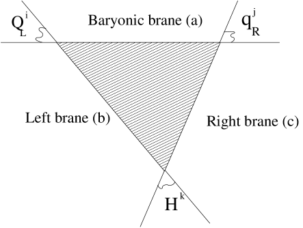
Figure 1: Yukawa coupling between two quarks of opposite chirality and a Higgs boson.

A paradigmatic example is presented in figure 1, where two quarks of opposite chirality couple to a Higgs boson. The worldsheet connecting the corresponding intersection has the topology of a disc, and involves three different boundary states. These are, in a target space perspective, branes $a$, $b$ and $c$, whose intersections localize the matter particles. Given such boundary conditions, there will exist an infinity of worldsheets satisfying them. In order to compute the instanton correction to our effective theory, however, we must concentrate on minimal action worldsheets that satisfy the classical equations of motion, and sum over topologically different sectors (see below). Each of these will contribute to the Yukawa coupling as something proportional to $exp(-S_{cl})$ so, naïvely, we would expect it to be weighted by exp($-A_{abc}$), where $A_{abc}$ is the worldsheet area.

As a result, Yukawa couplings will depend both on the D-brane positions and on the geometry of the underlying compact space. In terms of low energy quantities, these are characterized by open and closed string moduli v.e.v.’s. We have computed such dependence explicitly in the simple case of D-branes wrapping factorizable cycles on flat tori of arbitrary dimension. We have considered, as well, how these Yukawa are affected when more general configurations including non-vanishing B-field and Wilson lines are included. We find that Yukawa couplings have simple expressions in terms of complex theta functions with characteristics or, ultimately, in terms of multi-theta functions. This is somewhat analogous to the structure found for the Yukawa couplings of toroidal heterotic orbifold models as computed in [25]. No complex structure dependence appears in our Yukawa couplings, and the wrapping numbers of the D-branes configuration appear only through their intersection numbers on each subtorus. Thus given those intersection numbers one can immediately write down the Yukawa couplings for any toroidal intersecting brane model, there is no explicit dependence on the particular wrapping numbers of the given brane configuration. These general facts are illustrated by an explicit example presented below, based on D6-branes wrapping cycles on (an orientifold of) $T^{2}\times T^{2}\times T^{2}$ and with the chiral spectrum of the minimal supersymmetric standard model (MSSM). Explicit results for the Yukawa couplings are presented in this example, which reproduce the leading effect of one generation of quarks and leptons being much heavier than the first two.

The formulation we present can also be applied to some non-toroidal CY compactifications, i.e., certain elliptically fibered manifolds. In particular, the general class of elliptically fibered non-compact CY manifolds considered in ref.[17] which are mirror to complex cones over del Pezzo surfaces. Configurations of D6-branes wrapping cycles on the original CY have mirror configurations corresponding to D3-branes located at those singularities. A particularly simple case is that of D3-branes sitting at a ${\bf Z}_{3}$ singularity which is mirror to D6-branes wrapping cycles on an elliptically fibered non-compact CY manifold. Using our methods we compute the general form of Yukawa couplings in the wrapping D6-brane configuration and check that they match the Yukawa couplings known for D3-branes at a ${\bf Z}_{3}$ singularity.

The structure of this paper is as follows. In the next section we discuss the rôle of world-sheet instantons in the computation of Yukawa couplings in general intersecting brane configurations. In section 3 we explicitly compute the Yukawa couplings for intersecting configurations of D-branes wrapping cycles in a toroidal (orientifold) compactification. We also analyze the more general case in which a B-field and Wilson line backgrounds are added. Explicit expressions in terms of products of Jacobi complex theta functions with characteristics are given. In section 4 we discuss an explicit example yielding the chiral spectrum of the MSSM and provide the corresponding Yukawa couplings. A CY example (mirror to the case of D3-branes sitting on a ${\bf C}^{3}/{\bf Z}_{3}$ singularity) is briefly studied in section 5. We check there that the Yukawa couplings obtained from our method match the known results of the mirror. After performing our computations of section 3, we realized that they were intimately related to some previous work in the mathematical literature, in the very different context of homological mirror symmetry. Section 6 is devoted to briefly discuss such connection and, in particular, to show how computation of Yukawa couplings in intersecting D-brane models can be translated to the computation of Fukaya category in a generic symplectic manifold. Final comments and conclusions are left for section 7.

2 Intersecting brane models and Yukawa couplings

In this section we study intersecting D-brane models from a general viewpoint, reviewing some previous work on the field and collecting the necessary information for addressing the problem of Yukawa couplings. Most part of the effort on constructing phenomenologically appealing intersecting brane configurations has centered on simple toroidal and on orbifold/orientifold compactifications. However, main issues as, e.g., massless chiral spectrum and tadpole cancellation conditions, are of topological nature and thus easily tractable in more general compactifications where the metric may not be known explicitly. Following this general philosophy, we will introduce Yukawa couplings as arising from worldsheet instantons in a generic compactification. Although the specific computation of these worldsheet instantons needs the knowledge of the target space metric, many important features can be discussed at this more general level. In the next section we will perform such explicit computation in the simple case of toroidal compactifications, giving a hint of how these quantities may behave in a more general setup.

2.1 D-branes wrapping intersecting cycles

Consider type IIA string theory compactified on a six dimensional manifold ${\cal M}$. The building blocks of an intersecting brane configuration will be given by D6-branes filling four-dimensional Minkowski space-time and wrapping internal homology 3-cycles of ${\cal M}$. A specific configuration will thus consist of $K$ stacks of D6-branes, each stack $\alpha$ containing $N_{\alpha}$ coincident D6-branes whose worldvolume is given by ${\bf M_{4}}\times\Pi_{\alpha}\subset{\bf M_{4}}\times{\cal M}$, where $[\Pi_{\alpha}]\in H_{3}({\cal M},{\bf Z})$ is the corresponding homology class of such 3-cycle. The gauge theory arising from open string degrees of freedom will be localized on such D6-brane worldvolumes, giving rise to a total gauge group $\prod_{\alpha}U(N_{\alpha})$.

In addition, there will be some open strings modes arising from strings stretched between, say, stacks $\alpha$ and $\beta$. In case the corresponding 3-cycles $\Pi_{\alpha}$ and $\Pi_{\beta}$ intersect at a single point in the compact space ${\cal M}$, the lowest open string mode in the R sector will correspond to a chiral fermion localized at the four-dimensional intersection of $\alpha$ and $\beta$, transforming in the bifundamental representation of $U(N_{\alpha})\times U(N_{\beta})$ [1]. Notice that, since ${\cal M}$ is a compact manifold, $\Pi_{\alpha}$ and $\Pi_{\beta}$ will generically intersect several times. The number of such localized chiral fermions is given by the number of intersections $\#(\Pi_{\alpha}\cap\Pi_{\beta})$. This number is not, however, a topologically invariant quantity. Such invariant is constructed from subtracting the number of right-handed chiral fermions to left-handed ones, after what we obtain the intersection number $I_{\alpha\beta}\equiv[\Pi_{\alpha}]\cdot[\Pi_{\beta}]$, which give us the net number of chiral fermions in the $\alpha\beta$ sector.

As we are considering ${\cal M}$ to be compact, any configuration should satisfy some consistency conditions related to the propagation of Ramond-Ramond massless closed string fields on ${\cal M}$. These are the RR tadpole cancellation conditions which require the total RR charge of the configuration to vanish. In our case, the charge of a D6-brane $\alpha$ under the RR 7-form $C_{7}$ is classified by its associated 3-cycle homology cycle $[\Pi_{\alpha}]$. Hence, RR tadpoles amount to imposing that the sum of homology classes add up to zero [27]

$$\sum_{\alpha}N_{\alpha}[\Pi_{\alpha}]=0.$$ (1)

Additional RR sources may appear in general, such as O6-planes arising in orientifold compactifications or NS-NS background fluxes. Each of theses objects will have an associated 3-cycle homology class, so that RR conditions will be finally expressed again as the vanishing of the total homology class. It can be easily seen that RR tadpole conditions directly imply the cancellation of non-abelian $SU(N_{\alpha})^{3}$ anomalies. They also imply, by the mediation of a generalized Green-Schwarz mechanism [28, 29], the cancellation of mixed non-abelian and gravitational anomalies [3, 6, 8, 30].

So far, we have not imposed any particular constraint on our manifold ${\cal M}$, except that it must be compact so that we recover four-dimensional gravity at low energies. We may now require the closed string sector to be supersymmetric. This amounts to impose that ${\cal M}$, seen as a Riemannian manifold with metric $g$, has a holonomy group contained in $SU(3)$. Now, such a manifold can be equipped with a complex structure $J$ and a holomorphic volume 3-form $\Omega_{c}$ which are invariant under the holonomy group, i.e., covariantly constant. This promotes ${\cal M}$ to a Calabi-Yau three-fold, or ${\bf CY_{3}}$. Moreover, $g$ and $J$ define a Kähler 2-form $\omega$ which satisfies the following relation with the volume form

$$\frac{\omega^{3}}{3!}=\left(\frac{i}{2}\right)^{3}\Omega_{c}\wedge\overline{\Omega}_{c}.$$ (2)

Given a real 3-form $\Omega$ normalized as this, we can always take $\Omega_{c}=e^{i\theta}\Omega$ for any phase $\theta$ as a solution of (2). The Kähler form $\omega$ can also be complexified to $\omega_{c}$, by addition of a non-vanishing $B$-field. Both $\Omega$ and $\omega$ will play a central rôle when considering the open string sector.

Notice, however, that we have not imposed Hol$({\cal M})$ to be exactly $SU(3)$. We may consider, for instance, ${\cal M}=T^{2}\times{\bf K3}$, whose holonomy group is contained in $SU(2)$. In this case, there is not a unique invariant 3-form but two linearly independent ones, both satisfying (2). In general, the number of (real) covariantly constant 3-forms of ${\cal M}$ satisfying (2) indicates the amount of $D=4$ supersymmetries preserved under compactification. In a ${\bf CY_{3}}$ in the strict sense, with Hol$({\cal M})=SU(3)$, the gravity sector yields $D=4$ ${\cal N}=2$ under compactification, and this fact is represented by the existence of a unique complex volume form $e^{i\theta}\Omega$. Indeed, $\theta$ parametrizes the $U(1)$ of ${\cal N}=1$ superalgebras inside ${\cal N}=2$ [33]. Correspondingly, compactification on $T^{2}\times{\bf K3}$ yields a $D=4$ ${\cal N}=4$ gravity sector. There are some other consequences when considering manifolds of lower holonomy. For instance, Hol$({\cal M})=SU(3)$ implies that $b_{1}({\cal M})=0$ [31], while this might not be the case for lower holonomy, as the example $T^{2}\times{\bf K3}$ shows.

Let us now turn to the open string sector, represented by type IIA D6-branes. Intuitively, a dynamical object as a D-brane will tend to minimize its tension while conserving its RR charges. In our geometrical setup, this translates into the minimization of Vol($\Pi_{\alpha}$) inside the homology class $[\Pi_{\alpha}]$. A particular class of volume-minimizing objects are calibrated submanifolds, first introduced in [34]. The area or volume of such submanifolds can be computed by integrating on its $p$-volume a (real) closed $p$-form, named calibration, defined on the ambient space ${\cal M}$. Both $\Omega$ and $\omega$ are calibrations in a ${\bf CY_{3}}$. Submanifolds calibrated by $\Omega$ are named special Lagrangian [32] while those calibrated by $\omega$ are holomorphic curves. Being a 3-form, $\Omega$ will calibrate 3-cycles where D6-branes may wrap. A 3-cycle $\Pi_{\alpha}$ calibrated by Re($e^{i\theta}\Omega$) will have a minimal volume on $[\Pi_{\alpha}]$, given by Vol($\Pi_{\alpha}$) $=\int_{\Pi_{\alpha}}$ Re($e^{i\theta}\Omega$), and will be said to have phase $\theta$. We can also characterize such calibration condition by

$$\omega|_{\Pi_{\alpha}}\equiv 0\quad{\rm and}\quad{\rm Im}(e^{i\theta}\Omega)|_{\Pi_{\alpha}}\equiv 0.$$ (3)

The middle-homology objects that satisfy the first condition in (3) are named Lagrangian submanifolds and, although they are not volume minimizing, play a central rôle in symplectic geometry.

A D6-brane whose 3-cycle $\Pi_{\alpha}$ wraps a special Lagrangian (sL) submanifold does not only minimize its volume but, as shown in [35], also preserves some amount of supersymmetry. Being BPS stable objects of type IIA theory, it seems natural to consider D6-branes wrapping sL’s as building blocks of our intersecting brane configurations.

2.2 The rôle of worldsheet instantons

Being a BPS soliton of type IIA theory, a stack of $N_{\alpha}$ D6-brane wrapping a special Lagrangian submanifold $\Pi_{\alpha}$ will yield a $U(N_{\alpha})$ Supersymmetric Yang-Mills theory on its worldvolume. By simple dimensional reduction, the (inverse) gauge coupling constant can be seen to be proportional to Vol$(\Pi_{\alpha})$, which can be computed by integrating Re($e^{i\theta}\Omega$) on the corresponding homology cycle. A natural question is which amount of SUSY the D6-brane effective field theory will have by dimensional reduction down to $D=4$. The precise amount is again given by the number of independent real volume forms Re$(e^{i\theta}\Omega)$ that calibrate the 3-cycle. We may, however, seek for a more topological alternative method.

McLean’s theorem [36] states that the moduli space of deformations of a sL $\Pi_{\alpha}$ is a smooth manifold of (unobstructed) real dimension $b_{1}(\Pi_{\alpha})$. String theory complexifies this space, by adding the $b_{1}(\Pi_{\alpha})$ Wilson lines obtained from the gauge field $U(N_{\alpha})$ living on the worldvolume of the stack $\alpha$ In the low energy $D=4$ theory, this will translate into $b_{1}(\Pi_{\alpha})$ massless complex scalar fields in the adjoint of $U(N_{\alpha})$. Being in a supersymmetric theory, these fields will yield the scalar components of $D=4$ supermultiplets.

Let us consider the case ${\cal N}=1$ (for a clear discussion on this see, e.g., [37]). Here we find $b_{1}(\Pi_{\alpha})$ chiral multiplets $\phi_{j}$ in the adjoint of $U(N_{\alpha})$. Now, we may also seek to compute the superpotential $W$ of such ${\cal N}=1$ theory, which is a function on these chiral fields. By standard ${\cal N}=1$ considerations, this superpotential cannot be generated at any order in $\alpha^{\prime}$ perturbation theory, in accordance with the geometrical result of [36]. Indeed, such superpotential will be generated non-perturbatively by worldsheet instantons with their boundary in $\Pi_{\alpha}$.

Superpotentials generated non-perturbatively by worldsheet instantons were first considered in closed string theory [38], while the analogous problem in type IIA open string has been recently studied in [39, 40], in the context of open string mirror symmetry. The basic setup considered is a single D6-brane wrapping a sL $\Sigma$ in a ${\bf CY_{3}}$, with $b_{1}(\Sigma)>0$. Worldsheet instantons are constructed by considering all the possible embeddings of a Riemann surface ${\cal S}_{g}$ with arbitrary genus $g$ on the target space ${\cal M}$ and with boundary on $\Sigma$. In order to be topologically non-trivial, this boundary must be wrapped on the 1-cycles $\gamma_{j}$ that generate $b_{1}(\Sigma)$, thus coupling naturally to the corresponding chiral multiplets. Moreover, in order to deserve the name instanton, this euclidean worldsheet embedding must satisfy the classical equations of motion. This is guaranteed by considering embeddings which are holomorphic (or antiholomorphic) with respect to the target space complex structure, plus some extra constraints on the boundary (Dirichlet conditions). In geometrical terms, this means that worldsheet instantons must be surfaces calibrated by the Kähler form $\omega$. Calibration theory then assures the area minimality given such boundary conditions, which is what we would expect from naïve Nambu-Goto considerations. As a general result, it is found that the superpotential of D6-brane theories is entirely generated by instantons with the topology of a disc, while higher-genus instantons correspond to open string analogues of Gromov-Witten invariants.

So we find that, in case of ${\cal N}=1$ D6-branes on a ${\bf CY_{3}}$, great deal can be extracted from calibrated geometry of the target space ${\cal M}$. Whereas the gauge kinetic function $f_{ab}$ can be computed by evaluating the volume form $\Omega$ on the worldvolume $\Sigma$ of the brane, the superpotential can be computed by integrating the Kähler form $\omega$ on the holomorphic discs with boundary on $\Sigma$. The former only depends on the homology class $[\Sigma]\in H_{3}({\cal M},{\bf Z})$, and in the case of toroidal compactifications they have been explicitly computed in [11]. The latter, on the contrary, is given by a sum over the relative homology class $H_{2}^{D}({\cal M},\Sigma)$, that is, the classes of 2-cycles on ${\cal M}$ with boundary on $\Sigma$ (the superscript $D$ means that we only consider those 2-cycles with the topology of a disc). Notice that, ${\cal M}$ being compact, the disc instantons may wrap multiple times. Although in principle one may need the knowledge of the metric on ${\cal M}$ in order to compute both, much can be known about the form of the superpotential by considerations on Topological String Theory. For our purposes, we will contempt to stress two salient features:

• The superpotential depends on the target space metric only by means of Kähler moduli, and is independent of the complex structure [41].

• If we see those Kähler moduli as closed string parameters, the dependence of the superpotential is roughly of the form

  $$W=\pm\sum_{n=1}^{\infty}{e^{-n\Phi}\over n^{2}},$$ (4)

  where $n$ indexes the multiple covers of a disc with same boundary conditions, and $\Phi$ stands for the open string chiral superfield [42]. The $\pm$ sign corresponds to holomorphic and antiholomorphic maps, respectively.

Given these considerations, is easy to see that no superpotential will be generated for a chiral superfield associated to a 1-cycle $\gamma$ of $\Sigma$ which is also non-contractible in the ambient space ${\cal M}$, since no disc instanton exist that couples to such field. Notice that this could never happen in a ${\bf CY_{3}}$ on the strict sense, since in this case $b_{1}({\cal M})=0$. In manifolds with lower holonomy, however, it may well be the case that $b_{1}({\cal M})>0$, and so a D6-brane could have in its worldvolume a complex scalar not involved in the superpotential (4). We expect such scalars to give us the scalar content of the vector supermultiplet, thus indicating the degree of supersymmetry on the worldvolume effective theory. This seems an alternative method for computing the amount of supersymmetry that such a D6-brane preserves. A clear example of the above argument is constituted by ${\cal M}=T^{2}\times T^{2}\times T^{2}$ and $\Sigma$ a Lagrangian $T^{3}$ (the so called factorizable branes considered in the next section). Here, each of the three independent 1-cycles on $\Sigma$ is non-contractible in ${\cal M}$, so our SYM theory will yield three complex scalars not involved in the superpotential. But these scalar fields fill in the precise content of a $D=4$ ${\cal N}=4$ vector multiplet, which is the amount of SUSY those branes preserve.

2.3 Yukawa couplings in intersecting D-brane models

Up to now, we have only considered superpotentials arising from one single stack of D6-branes. In the intersecting brane world picture we have given above, however, chiral matter in the bifundamental arises from the intersection of two stacks of branes, each with a different gauge group. It thus seems that, in order to furnish a realistic scenario, several stacks of branes are needed. In fact, given the semi-realistic model-building considered up to now, it seems that a minimal number of four stacks of branes are necessary in order to accommodate the chiral content of the Standard Model in bifundamentals [6]. These stacks have been named as Baryonic (a), Left (b), Right (c) and Leptonic (d), in account of the global quantum numbers they carry. The gauge theory they initially yield is $U(3)\times U(2)\times U(1)\times U(1)$, which arises from stack multiplicities $N_{a}=3$, $N_{b}=2$, $N_{c}=1$ and $N_{d}=1$. Although this yields extra abelian gauge factors, their gauge bosons may become massive by coupling to closed string RR fields, showing up in the low energy limit as global $U(1)$ symmetries [6]. Standard Model chiral fermions will naturally arise from pairs of intersecting stacks. For instance, left-handed quarks will arise from the intersection points of baryonic and left stacks, and so on. This scenario has been depicted schematically in figure 2. For short reviews on this subject see [43].

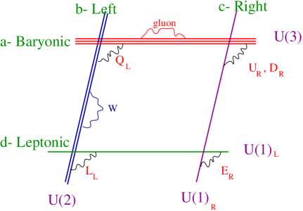
(a)	(b)

Figure 2: The Standard Model at intersecting D-branes. a) Four stacks of branes, baryonic, left, right and leptonic are needed to get all quark and leptons at the intersections. b) The SM branes may be wrapping cycles on a, e.g., CY manifold, with appropriate intersections so as to yield the SM chiral spectrum.

Notice that considering a full D6-brane configuration instead of one single brane makes the supersymmetry discussion more involved. Although each of the components of the configuration (i.e., each stack of D6-branes) is wrapping a special Lagrangian cycle and thus yields a supersymmetric theory on its worldvolume, it may well happen that two cycles do not preserve a common supersymmetry. In a ${\bf CY_{3}}$ of $SU(3)$ holonomy this picture is conceptually quite simple. There only exist one family of real volume forms $\Omega$ parametrized by a phase $e^{i\theta}$. Two sL’s $\Pi_{\alpha}$, $\Pi_{\beta}$ will preserve the same supersymmetry if they are calibrated by the same real 3-form, that is, if $\theta_{\alpha}=\theta_{\beta}$ in (3). In this case, a chiral fermion living at the intersection $\Pi_{\alpha}\cap\Pi_{\beta}$ will be accompanied by a complex scalar with the same quantum numbers, filling up a ${\cal N}=1$ chiral multiplet . In manifolds of lower holonomy, however, there are far more possibilities, since many more SUSY’s are involved. Consideration of such possibilities lead to the idea of Quasi-Supersymmetry in [11, 12] (see [45] for related work). In order to simplify our discussion, we will suppose that all the branes preserve the same ${\cal N}=1$ superalgebra, although our results in the next section seem totally independent of this assumption.

It was noticed in [4] that, in the context of intersecting brane worlds, Yukawa couplings between fields living at brane intersections will arise from worldsheet instantons involving three different boundary conditions (see figure 3). Let us, for instance, consider a triplet of D6-brane stacks and suppose them to be the Baryonic, Left and Right stacks, wrapping the sL’s $\Pi_{a}$, $\Pi_{b}$ and $\Pi_{c}$ respectively. By computing the quantum numbers of the fields at the intersections, we find that fields $Q_{L}^{i}\in\Pi_{a}\cap\Pi_{b}$ can be identified with Left-handed quarks, $q_{R}^{j}\in\Pi_{c}\cap\Pi_{a}$ with Right-handed quarks and finally $H^{k}\in\Pi_{b}\cap\Pi_{c}$ with Higgs particles . A Yukawa coupling in SM physics will arise from a coupling between these three fields. In our context, such trilinear coupling will arise from the contribution of open worldsheet instantons with the topology of a disc and with three insertions on its boundary. Each of these insertions corresponds to an open string twisted vertex operators that changes boundary conditions, so that finally three different boundaries are involved in the amplitude.

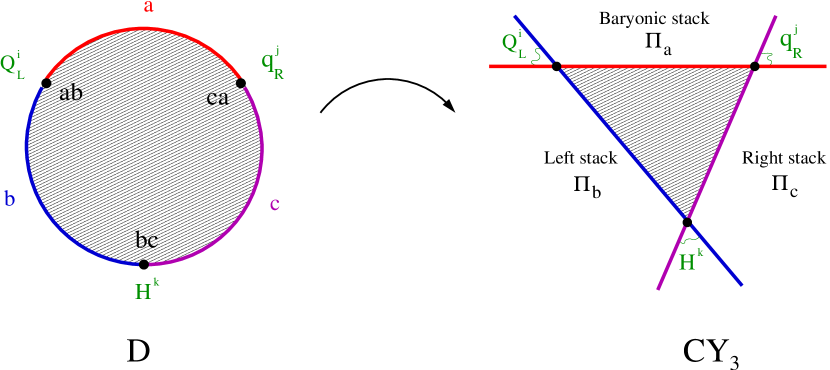
Figure 3: Yukawa couplings as euclidean maps from the worldsheet.

From the target space perspective, such amplitude will arise from an (euclidean) embedding of the disc in the compact manifold ${\cal M}$, with each vertex operator mapped to the appropriate intersection of two branes (generically a fixed point in ${\cal M}$) and the disc boundary between, say, $ca$ and $ab$ to the worldvolume of the D6-brane stack $a$, etc. Such mapping $D\rightarrow{\cal M}$ has been schematically drawn in figure 3.

Notice that an infinite family of such maps exist. However, only a subfamily satisfies the classical equations of motion, thus corresponding to true semiclassical instanton configurations. As expected, these correspond to holomorphic embeddings of $D$ on ${\cal M}$ with the boundary conditions described above. Just as in the previous case of one single D6-brane, these instantons correspond to surfaces calibrated by the Kähler form $\omega$, hence of minimal area. In the specific setup discussed in [4], the geometry of intersecting brane worlds is reduced to each stack wrapping (linear) 1-cycles on a $T^{2}$. It is thus easy to see that in this case the target space worldsheet instanton has a planar triangular shape. This, however, will not be the general shape for a holomorphic curve, even in the familiar case of higher dimensional tori with a flat metric (see appendix A).

More concretely, we expect the Yukawa couplings between the fields $Q_{L}^{i}$, $q_{R}^{j}$ and $H^{k}$ to be roughly of the form:

$$Y_{ijk}=h_{qu}\sum_{\vec{n}\pm\in H_{2}^{D}({\cal M},\cup_{\alpha}\Pi_{\alpha},ijk)}{d_{\vec{n}}\ e^{-{A_{ijk}(\vec{n})\over 2\pi\alpha^{\prime}}}e^{-2\pi i\phi_{ijk}(\vec{n})}}.$$ (5)

Here $\vec{n}$ is an element of the relative homology group $H_{2}({\cal M};\cup_{\alpha}\Pi_{\alpha},{\bf Z})$, that is, a 2-cycle in the Calabi-Yau ${\cal M}$ ending on $\cup_{\alpha}\Pi_{\alpha}=\Pi_{a}\cup\Pi_{b}\cup\Pi_{c}$. We further impose this 2-cycle to have the topology of a disc, and to connect the intersections $i\in\Pi_{a}\cap\Pi_{b}$, $j\in\Pi_{c}\cap\Pi_{a}$, $k\in\Pi_{b}\cap\Pi_{c}$ following the boundary conditions described above. Given such a topological sector indexed by $\vec{n}$, we expect a discrete number of holomorphic discs to exist, and we have indicated such multiplicity by $d_{\vec{n}}$. The main contribution comes from the exponentiation of $A_{ijk}(\vec{n})=\int_{\vec{n}}\omega$, which is the target-area of such ’triangular’ surface, whereas $\phi_{ijk}(\vec{n})$ is the phase the string endpoints pick up when going around the disc boundary $\partial D$ (see next section). As in (4), the sign depends on the discs wrapping holomorphic or antiholomorphic maps. Finally, $h_{qu}$ stands for the contribution coming from quantum corrections, i.e., fluctuations around the minimal area semiclassical solution. Just as in the closed string case [25], we expect such contributions to factorize from the infinite semiclassical sum.

At this point one may wonder what is the detailed mechanism by which the chiral fermions get their mass. That is, one may want to understand what is the D-brane analog of Higgs mechanism in this intersecting brane picture. The right answer seems to be brane recombination, studied from a geometrical viewpoint by Joyce [46], and later in terms of D-brane physics in [44, 47, 48]. The connection of such phenomenon to the SM Higgs mechanism was addressed in [12]. Here we will briefly sketch this line of thought from a general viewpoint. Consider two D6-branes wrapping two sL’s $\Pi_{\alpha}$ and $\Pi_{\beta}$ on a ${\bf CY_{3}}$ ${\cal M}$, and further assume that they have the same phase, i.e., both are calibrated by the same real volume form $\Omega_{\theta}$ and thus preserve (at least) a common ${\cal N}=1$ in $D=4$. From the geometrical viewpoint, they lie in a marginal stability wall of ${\cal M}$. This implies that we can marginally deform our configuration by ’smoothing out’ the intersections $\Pi_{a}\cap\Pi_{\beta}$, combining the previous two sL’s into a third one $\Pi_{\gamma}$. This family of deformations will all be calibrated by the same real volume form $\Omega_{\theta}$, so that the total volume or tension of the system will be invariant. From the field theory point of view, this deformation translates into giving non-vanishing v.e.v.’s to the massless scalar fields at the intersections.

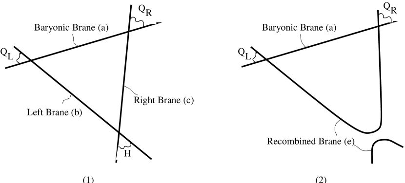
Figure 4: Picture of the recombination. (1) Before the recombination, the worldsheet instantons connecting the $Q_{L}$, $Q_{R}$ and Higgs multiplets corresponds to holomorphic discs with their boundaries embedded in three different branes. (2) After giving a v.e.v. to $H$, stacks $b$ and $c$ have recombined into a third one $e$. If the recombination is soft enough, the number of chiral fermions at the intersections will not vary. However, they will get mass terms by holomorphic discs that connect fermions of opposite chirality, having its boundary on stacks $a$ and $e$.

Let us then consider the recombination of our SM stacks $b$ and $c$ into a third one $e$. By the above discussion, this correspond to giving a v.e.v. to Higgs multiplets living on $\Pi_{b}\cap\Pi_{c}$, so we expect that this implies a mass term for our chiral fermions. Indeed, in intersecting brane worlds, the chirality condition that prevents fermions from getting a mass is encoded in the non-vanishing topological intersection number of two branes, such as $[\Pi_{a}]\cdot[\Pi_{b}]$, $[\Pi_{c}]\cdot[\Pi_{a}]\neq 0$ that give us the number of net chiral quarks. Notice, however, that upon brane recombination, we will have

$$\left|[\Pi_{a}]\cdot[\Pi_{e}]\right|=\left|[\Pi_{a}]\cdot([\Pi_{b}]+[\Pi_{c}])\right|\leq\left|[\Pi_{a}]\cdot[\Pi_{b}]\right|+\left|[\Pi_{a}]\cdot[\Pi_{c}]\right|,$$ (6)

which implies that the number of ’protected’ chiral fermions decreases if $[\Pi_{a}]\cdot[\Pi_{b}]$ and $[\Pi_{a}]\cdot[\Pi_{c}]$ have opposite sign, that is, yield fermions of opposite chirality. In realistic models we usually have $[\Pi_{a}]\cdot[\Pi_{e}]=0$, so we expect every quark to get a mass.

Since we are in a supersymmetric situation, we are allowed to perform an arbitrary small deformation from the initial configuration where the branes were not recombined. Upon such ’soft recombination’, the actual number of intersections will not change, i.e., $\#(\Pi_{a}\cap\Pi_{e})=\#(\Pi_{a}\cap\Pi_{b})+\#(\Pi_{a}\cap\Pi_{c})$. This implies that left and right-handed quarks will still be localized at intersections of $a$ and $e$. They will get, however, a mass term from a worldsheet instanton connecting each pair of them, now involving only two different boundaries. This situation has been illustrated in figure 4.

Before closing this section, let us mention that the discussion of Yukawa couplings, involving three or more stacks of branes, is intimately related to the previous discussion involving one single D-brane. Indeed, given a supersymmetric configuration of three stacks of D6-branes, we could think of slightly smoothing out each single intersection between each pair of them, thus recovering one single D6-brane wrapping a special Lagrangian. Now, by our general considerations of the superpotential of one single brane, we know that such superpotential will only depend on closed string Kähler moduli, and that will have the general form (4). We expect the same results to hold in the case of the superpotential involving Yukawa couplings before recombination. In the next section we will compute such trilinear couplings for the simple case of Lagrangian $T^{n}$ wrapping n-cycles on $T^{2n}$, and see that they indeed satisfy such conditions.

3 The general form of Yukawa couplings in toroidal models

In this section we derive the general expression for Yukawa couplings in toroidal and factorizable intersecting brane configurations. By this we mean that the compact manifold will be a factorizable flat torus ${\cal M}=T^{2n}=\otimes_{r=1}^{n}T_{r}^{2}$, whereas D-branes will be wrapping Lagrangian factorizable $n$-cycles, that is, those that can be expressed as a product of $n$ 1-cycles $\Pi_{\alpha}=\otimes_{r=1}^{n}(n_{\alpha}^{r},m_{\alpha}^{r})$, one on each $T^{2}$. Such $n$-cycles have the topology of $T^{n}$ and, if we minimize their volume in its homology class, they are described by hyperplanes quotiented by a torus lattice. This implies, in particular, that the intersection number between two cycles is nothing but the (signed) number of intersections, that is, $\#(\Pi_{\alpha}\cap\Pi_{\beta})=|[\Pi_{\alpha}]\cdot[\Pi_{\beta}]|$. Such class of configurations are known in the literature as branes at angles [1]. Although our discussion in the previous section seems to indicate that the interesting case to study is $n=3$, realistic models may be constructed involving also $n=1,2$ [3]. For completeness, we derive our results for arbitrary $n$.

3.1 Computing Yukawas on a $T^{2}$

The simplest case when computing a sum of worldsheet instantons comes, as usual, from D-branes wrapping 1-cycles in a $T^{2}$, that is, branes intersecting at one angle. Let us then consider three of such branes, given by

$$\begin{array}[]{ccc}\quad[\Pi_{a}]=[(n_{a},m_{a})]&\rightarrow&z_{a}=R\cdot(n_{a}+\tau m_{a})\cdot x_{a}\\ \quad[\Pi_{b}]=[(n_{b},m_{b})]&\rightarrow&z_{b}=R\cdot(n_{b}+\tau m_{b})\cdot x_{b}\\ \quad[\Pi_{c}]=[(n_{c},m_{c})]&\rightarrow&z_{c}=R\cdot(n_{c}+\tau m_{c})\cdot x_{c}\end{array}$$ (7)

where $(n_{\alpha},m_{\alpha})\in{\bf Z}^{2}$ denote the 1-cycle the brane $\alpha$ wraps on $T^{2}$. Since the manifold of minimal volume in this homology class is given by a straight line with the proper slope, we can associate a complex number $z_{\alpha}$ to each brane, which stands for a segment of such 1-cycle in the covering space ${\bf C}$. Here $\tau$ is the complex structure of the torus and $x_{\alpha}\in{\bf R}$ an arbitrary number. We fix the area of $T^{2}$ (the Kähler structure, if we ignore the possibility of a B-field) to be $A=R^{2}\ {\rm Im\,}\tau$. The triangles that will contribute to a Yukawa coupling involving branes $a$, $b$ and $c$ will consist of those triangles whose sides lie on such branes, hence of the form $(z_{a},z_{b},z_{c})$. To be an actual triangle, however, we must impose that it closes, that is

$$z_{a}+z_{b}+z_{c}=0.$$ (8)

Since $n_{\alpha}$, $m_{\alpha}$ can only take integer values, (8) can be translated into a Diophantine equation, whose solution is

$$\begin{array}[]{c}x_{a}=\left(I_{bc}/d\right)\cdot x\\ x_{b}=\left(I_{ca}/d\right)\cdot x\\ x_{c}=\left(I_{ab}/d\right)\cdot x\end{array} \ {\rm with} \begin{array}[]{c}x=\left(x_{0}+l\right)\\ x_{0}\in{\bf R},\ l\in{\bf Z}\\ d=g.c.d.\left(I_{ab},I_{bc},I_{ca}\right)\end{array}$$ (15)

where $I_{\alpha\beta}=[\Pi_{\alpha}]\cdot[\Pi_{\beta}]=n_{\alpha}m_{\beta}-n_{\beta}m_{\alpha}$ stands for the intersection number of branes $\alpha$ and $\beta$, and $x_{0}$ is a continuous parameter which is fixed for a particular choice of intersection points and brane positions, being a particular solution of (8). If, for instance, we choose branes $a$, $b$ and $c$ to intersect all at the same point, then we must take $x_{0}=0$. The discrete parameter $l$ then arises from triangles connecting different points in the covering space ${\bf C}$ but the same points under the lattice identification that defines our $T^{2}$. In the language of the section 2, $l$ indexes the elements of the relative homology class $H_{2}^{D}(T^{2},\Pi_{a}\cup\Pi_{b}\cup\Pi_{c},ijk)$. We thus see that a given Yukawa coupling gets contributions from an infinite (discrete) number of triangles indexed by $l$.

Let us describe the specific values that $x_{0}$ can take. First notice that each pair of branes will intersect several times, each of them in a different point of $T^{2}$. Namely, we can index such intersection points by

$$\begin{array}[]{cc}i=0,1,\dots,|I_{ab}|-1,&i\in\Pi_{a}\cap\Pi_{b}\\ j=0,1,\dots,|I_{ca}|-1,&j\in\Pi_{c}\cap\Pi_{a}\\ k=0,1,\dots,|I_{bc}|-1,&k\in\Pi_{b}\cap\Pi_{c}\end{array}$$ (16)

In general, $x_{0}$ must depend on the particular triplet $(i,j,k)$ of intersection points and on the relative positions of the branes. For simplicity, let us take the triplet of intersections $(0,0,0)$ to correspond to a triangle of zero area. That is, we are supposing that the three branes intersect at a single point, which we will choose as the origin of the covering space (see figure 5). Then it can be shown that, given the appropriate indexing of the intersection points, there is a simple expression for $x_{0}$ given by

$$x_{0}(i,j,k)=\frac{i}{I_{ab}}+\frac{j}{I_{ca}}+\frac{k}{I_{bc}},$$ (17)

where $i$, $j$ and $k$ are defined as in (16) . In this latter expression we are supposing that $d=1$, that is, that $I_{ab}$, $I_{bc}$ and $I_{ca}$ are coprime integers. This guarantees that there exist a triangle connecting every triplet $(i,j,k)$, and also a simple expression for $x_{0}$. The case $d\neq 1$ will be treated below. An illustrative example of the above formula is shown in figure 5, where a triplet of 1-cycles intersecting at the origin have been depicted, both in a square torus and in its covering space, and the intersections have been indexed in the appropriate manner so that (17) holds.

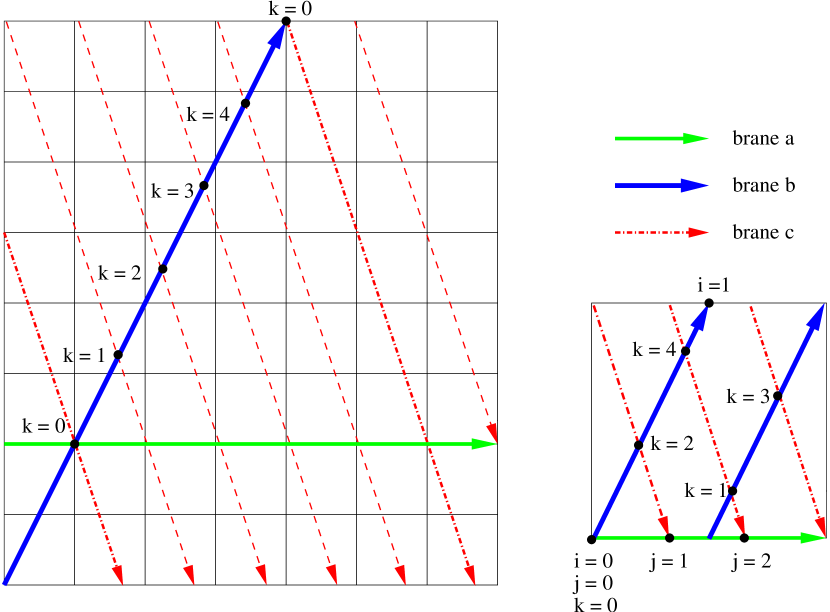
Figure 5: Relevant intersections and triangles for the three 1-cycles $(n_{a},m_{a})=(1,0)$, $(n_{b},m_{b})=(1,2)$ and $(n_{c},m_{c})=(1,-3)$. In the left figure we have depicted these 1-cycles intersecting on the covering space ${\bf C}$. The dashed lines represent various images of the brane $c$ under torus translations. The indexing of the $bc$ intersections by the integer $k$ coincides with expressions (15) and (17). In the right figure we have depicted a single fundamental region of the torus, and have indexed every intersection. Notice that we have chosen that all branes intersect at the origin, and the special choice of a square lattice for the complex structure. The results, however, are general.

What if these branes do not intersect all at the origin? Let us consider shifting the positions of the three branes by the translations $\epsilon_{a}$, $\epsilon_{b}$ and $\epsilon_{c}$, where $\epsilon_{\alpha}$ is the transversal distance of the brane $\alpha$ from the origin measured in units of $A/||\Pi_{\alpha}||$, in clockwise sense from the direction defined by $\Pi_{\alpha}$. Then is easy to see that (17) is transformed to

$$x_{0}(i,j,k)=\frac{i}{I_{ab}}+\frac{j}{I_{ca}}+\frac{k}{I_{bc}}+\frac{I_{ab}\epsilon_{c}+I_{ca}\epsilon_{b}+I_{bc}\epsilon_{a}}{I_{ab}I_{bc}I_{ca}}.$$ (18)

Notice, however, that we can absorb these three parameters into only one, to be defined as $\tilde{\epsilon}=\frac{I_{ab}\epsilon_{c}+I_{ca}\epsilon_{b}+I_{bc}\epsilon_{a}}{I_{ab}I_{bc}I_{ca}}$. This was to be expected since, given the reparametrization invariance present in $T^{2}$, we can always choose branes $b$ and $c$ to intersect at the origin, and then the only freedom comes from shifting the brane $a$ away from this point.

Given this solution, now we can compute the areas of the triangles whose vertices lie on the triplet of intersections $(i,j,k)$ (we will say that this triangle ’connects’ these three intersections), by using the well-known formula

$$A(z_{a},z_{b})=\frac{1}{2}\sqrt{|z_{a}|^{2}\cdot|z_{b}|^{2}-({\rm Re\,}z_{a}\bar{z_{b}})^{2}}.$$ (19)

Then we find that

$$A_{ijk}(l) = \frac{1}{2}(2\pi)^{2}A|I_{ab}I_{bc}I_{ca}|\ (x_{0}(i,j,k)+l)^{2}$$ (20)

$$= \frac{1}{2}(2\pi)^{2}A|I_{ab}I_{bc}I_{ca}|\left(\frac{i}{I_{ab}}+\frac{j}{I_{ca}}+\frac{k}{I_{bc}}+\tilde{\epsilon}+l\right)^{2},$$

where $A$ represents the Kähler structure of the torus, and we have absorbed all the shift parameters into $\tilde{\epsilon}$. The area of such triangle may correspond to either an holomorphic or an antiholomorphic map from the disc. From (15), we see this depends on the sign of $I_{ab}I_{bc}I_{ca}$, so we must add a real phase $\sigma_{abc}={\rm sign}(I_{ab}I_{bc}I_{ca})$ to the full instanton contribution.

We can finally compute the corresponding Yukawa coupling for the three particles living at the intersections $(i,j,k)$:

$$Y_{ijk}\sim\sigma_{abc}\sum_{l\in{\bf Z}}{\rm exp}\left(-{A_{ijk}(l)\over 2\pi\alpha^{\prime}}\right)$$ (21)

This last quantity can be naturally expressed in terms of a modular theta function, which in their real version are defined as

$$\vartheta\left[\begin{array}[]{c}\delta\\ \phi\end{array}\right](t)=\sum_{l\in{\bf Z}}q^{\frac{1}{2}(\delta+l)^{2}}\ e^{2\pi i(\delta+l)\phi},\ \ q=e^{-2\pi t}.$$ (22)

Indeed, we find that (21) can be expressed as such theta function with parameters

$$\delta = \frac{i}{I_{ab}}+\frac{j}{I_{ca}}+\frac{k}{I_{bc}}+\frac{I_{ab}\epsilon_{c}+I_{ca}\epsilon_{b}+I_{bc}\epsilon_{a}}{I_{ab}I_{bc}I_{ca}},$$ (23)

$$\phi = 0,$$ (24)

$$t = \frac{A}{\alpha^{\prime}}|I_{ab}I_{bc}I_{ca}|.$$ (25)

3.1.1 Adding a B-field and Wilson lines

It is quite remarkable that we can express our Yukawa couplings in terms of a simple theta function. However, reached this point we could ask ourselves why it is such a specific theta function. That is, we are only considering the variable $t$ as a real number, instead of a more general parameter $\kappa\in{\bf C}$, and we are always setting $\phi=0$. These two constraints imply that our theta functions are strictly real. From both the theoretical an phenomenological point of view, however, it would be interesting to have a Yukawa defined by a complex number.

These two constraints come from the fact that we have considered very particular configurations of branes at angles. First of all we have not considered but tori where the B-field was turned off. This translates into a very special Kähler structure, where only the area plays an important rôle. In general, if we turn on a B-field, the string sweeping a two-dimensional surface will not only couple to the metric but also to this B-field. In a $T^{2}$, since the Kähler structure is the complex field

$$J=B+iA,$$ (26)

we expect that, by including a B-field, our results (25) will remain almost unchanged, with the only change given by the substitution $A\rightarrow(-i)J$. this amounts to changing our parameter $t$ to a complex one defined as

$$\kappa=\frac{J}{\alpha^{\prime}}|I_{ab}I_{bc}I_{ca}|.$$ (27)

Our second generalization is including Wilson lines around the compact directions that the D-branes wrap. Indeed, when considering D-branes wrapping 1-cycles on a $T^{2}$, we can consider the possibility of adding a Wilson line around this particular one-cycle. Since we do not want any gauge symmetry breaking, we will generally choose these Wilson lines to correspond to group elements on the centre of our gauge group, i.e., a phase .

Let us then consider a triangle formed by D-branes $a$, $b$ and $c$ each wrapped on one different 1-cycle of $T^{2}$ and with Wilson lines given by the phases $exp(2\pi i\theta_{a})$, $exp(2\pi i\theta_{b})$ and $exp(2\pi i\theta_{c})$, respectively. The total phase that an open string sweeping such triangle picks up depends on the relative longitude of each segment, and is given by

$$e^{2\pi ix_{a}\theta_{a}}\cdot e^{2\pi ix_{b}\theta_{b}}\cdot e^{2\pi ix_{c}\theta_{c}}=e^{2\pi i\left(I_{bc}\theta_{a}+I_{ca}\theta_{b}+I_{ab}\theta_{c}\right)x}.$$ (28)

Finally, we will consider both possibilities: having a B-field and some Wilson lines. In order to express our results we need to consider the complex theta function with characteristics, defined as

$$\vartheta\left[\begin{array}[]{c}\delta\\ \phi\end{array}\right](\kappa)=\sum_{l\in{\bf Z}}e^{\pi i(\delta+l)^{2}\kappa}\ e^{2\pi i(\delta+l)\phi}.$$ (29)

Our results for the Yukawa couplings can then be expressed as such a function with parameters

$$\delta = \frac{i}{I_{ab}}+\frac{j}{I_{ca}}+\frac{k}{I_{bc}}+\frac{I_{ab}\epsilon_{c}+I_{ca}\epsilon_{b}+I_{bc}\epsilon_{a}}{I_{ab}I_{bc}I_{ca}},$$ (30)

$$\phi = I_{ab}\theta_{c}+I_{ca}\theta_{b}+I_{bc}\theta_{a},$$ (31)

$$\kappa = \frac{J}{\alpha^{\prime}}|I_{ab}I_{bc}I_{ca}|.$$ (32)

3.1.2 Orientifolding the torus

From a phenomenological point of view, it is often interesting to deal with a slight modification of the above toroidal model, which consist on performing an orientifold projection on the torus. Namely, we quotient the theory by $\Omega{\cal R}$, where $\Omega$ is the usual worldsheet orientation reversal and ${\cal R}:z\mapsto\bar{z}$ is a ${\bf Z}_{2}$ action on the torus. This introduces several new features, the most relevant for our discussion being

• There appears a new object: the O-plane, which lies on the horizontal axis described by $\{{\rm Im\,}z=0\}$ in the covering space ${\bf C}$.

• In order to consider well-defined constructions, for each D-brane $a$ in our configuration we must include its image under $\Omega{\cal R}$, denoted by $\Omega{\cal R}a$ or $a^{*}$. These mirror branes will, generically, wrap a cycle $[\Pi_{a^{*}}]$ different from $[\Pi_{a}]$, of course related by the action of ${\cal R}$ on the homology of the torus.

This last feature has a straightforward consequence, which is the proliferation of sectors as $ab$, $ab^{*}$, etc. Indeed, if we think of a configuration involving D-branes $a$, $b$ and $c$, we can no longer bother only about the triangle $abc$, but we must also consider $abc^{*}$, $ab^{*}c$ and $ab^{*}c^{*}$ triangles (the other possible combinations are mirror pairs of these four). Once specified the wrapping numbers of the triangle $abc$ all the others are also fixed. Since our formulae for the Yukawas are not very sensitive to the actual wrapping number of the 1-cycles but only to the intersection numbers, we do not expect these to appear in the final expression. Notice, however, that if we specify the position of the brane $a$ the position of its mirror $a^{*}$ is also specified. Hence, shifts of branes should be related in the four triangles. This can be also deduced from the first item above. Since we have a rigid object lying in one definite 1-cycle, which is the O-plane, translation invariance is broken in the directions transverse to it, so we have to specify more parameters in a certain configuration. In this case of $T^{2}$ this means that if we consider that the three branes intersect at one point, we must specify the ’height’ (${\rm Im\,}z$) of such intersection.

So our problem consists of, given the theta function parameters of the triangle $abc$, find those of the other three triangles. First notice that, if we actually consider the three branes $a$, $b$ and $c$ intersecting at one point, then the same will happen for the triangles $abc^{*}$, $ab^{*}c$ and $ab^{*}c^{*}$. Then by our previous results on triangles on a plain $T^{2}$ we see that the theta parameters will be given by

$$\delta_{abc} = \frac{i}{I_{ab}}+\frac{j}{I_{ca}}+\frac{k}{I_{bc}},$$ (33)

$$\kappa_{abc} = \frac{J}{\alpha^{\prime}}|I_{ab}I_{bc}I_{ca}|,$$ (34)

for the $abc$ triangle and

$$\delta_{ab^{*}c} = \frac{i^{*}}{I_{ab^{*}}}+\frac{j}{I_{ca}}+\frac{k^{*}}{I_{b^{*}c}},$$ (35)

$$\kappa_{ab^{*}c} = \frac{J}{\alpha^{\prime}}|I_{ab^{*}}I_{b^{*}c}I_{ca}|,$$ (36)

for the $ab^{*}c$ triangle, etc. Notice that $i$ and $i^{*}$ are different indices which label, respectively, $ab$ and $ab^{*}$ intersections.

A general configuration will not, however, contain every triplet of branes intersecting at one point, and will also contain non-zero Wilson lines. As mentioned, once specified the relative positions and Wilson lines of the triangle $abc$ all the other triangles are also specified. By simple inspection we can see that a general solution is given by the parameters

$$\delta_{abc} = \frac{i}{I_{ab}}+\frac{j}{I_{ca}}+\frac{k}{I_{bc}}+\frac{I_{ab}\epsilon_{c}+I_{ca}\epsilon_{b}+I_{bc}\epsilon_{a}}{I_{ab}I_{bc}I_{ca}},$$ (37)

$$\phi_{abc} = I_{ab}\theta_{c}+I_{ca}\theta_{b}+I_{bc}\theta_{a},$$ (38)

for the triangle $abc$, and the parameters

$$\delta_{ab^{*}c} = \frac{i^{*}}{I_{ab^{*}}}+\frac{j}{I_{ca}}+\frac{k^{*}}{I_{b^{*}c}}+\frac{I_{ab^{*}}\epsilon_{c}+I_{ca}\epsilon_{b^{*}}+I_{b^{*}c}\epsilon_{a}}{I_{ab^{*}}I_{b^{*}c}I_{ca}},$$ (39)

$$\phi_{ab^{*}c} = I_{ab^{*}}\theta_{c}+I_{ca}\theta_{b^{*}}+I_{b^{*}c}\theta_{a},$$ (40)

for the triangle $ab^{*}c$, and similarly for the other two triangles. Here we have defined

$$\begin{array}[]{c}\epsilon_{\alpha^{*}}=-\epsilon_{\alpha}\\ \theta_{\alpha^{*}}=-\theta_{\alpha}\end{array} \alpha=a,b,c.$$ (43)

3.1.3 The non-coprime case

Up to now, we have only consider a very particular class of Yukawa couplings: those that arise from intersecting D-branes wrapping 1-cycles on a $T^{2}$. Furthermore, we have also assumed the constraint $d=g.c.d.(I_{ab},I_{bc},I_{ca})=1$, that is, that the three intersection numbers are coprime. The non-coprime case is, however, the most interesting from the phenomenological point of view. In this section, we will try to address the non-coprime case. Although no explicit formula is given, we propose an ansatz that has been checked in plenty of models.

A particular feature of the configurations where $d>1$ is that not every triplet of intersections $(i,j,k)$ is connected by a triangle. Indeed, from solution (15) we see that a pair of intersections $(i,j)$ from $(ab,ca)$ will only couple to $|I_{bc}|/d$ different $bc$ intersections, same for the other pairs. Similarly, one definite intersection from $bc$ will couple to $|I_{ab}I_{ca}|/d^{2}$ $(i,j)$ pairs of $(ab,ca)$ intersections. This can be seen in figure 6, where a particular example of non-coprime configuration is shown.

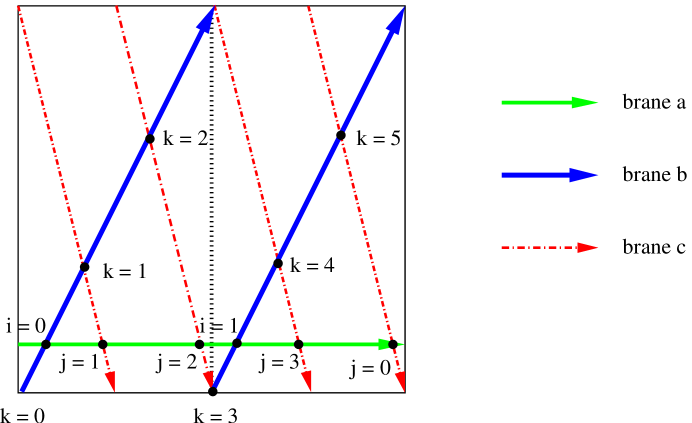
Figure 6: Relevant intersections and triangles for the three 1-cycles $(n_{a},m_{a})=(1,0)$, $(n_{b},m_{b})=(1,2)$ and $(n_{c},m_{c})=(1,-4)$. Notice that the fundamental region of the torus has two identical regions, exactly matching with $d=g.c.d.(I_{ab},I_{bc},I_{ca})=2$. Also notice that a triangle exists connecting the vertices $(i,j,k)$ if and only if $i+j+k=$ even.

In this same figure we can appreciate another feature of these configurations, which is that the fundamental region of the torus divides in $d$ identical copies. That is, the intersection pattern of any of these regions exactly matches the others. This is a direct consequence from the Diophantine solution (15).

Let us now formulate the ansatz for this more general class of configurations. It consist of two points:

• A Yukawa coupling can be expressed as a complex theta function, whose parameters are

  $$\delta = \frac{i}{I_{ab}}+\frac{j}{I_{ca}}+\frac{k}{I_{bc}}+\frac{d\cdot\left(I_{ab}\epsilon_{c}+I_{ca}\epsilon_{b}+I_{bc}\epsilon_{a}\right)}{I_{ab}I_{bc}I_{ca}}+\frac{s}{d},$$ (44)

  $$\phi = \left(I_{ab}\theta_{c}+I_{ca}\theta_{b}+I_{bc}\theta_{a}\right)/d,$$ (45)

  $$\kappa = \frac{J}{\alpha^{\prime}}{|I_{ab}I_{bc}I_{ca}|\over d^{2}}$$ (46)

  where $s\equiv s(i,j,k)\in{\bf Z}$ is a linear function on the integers $i$, $j$ and $k$.

• A triplet of intersections $(i,j,k)$ is connected by a family of triangles, that is, has a non-zero Yukawa, if and only if

  $$i+j+k\equiv 0\ {\rm mod\ }d.$$ (47)

Notice that this ansatz correctly reduces to the previous solution in the coprime case, i.e., when $d=1$. Indeed, in that case the actual value of $s$ becomes unimportant for the evaluation of the theta function and the condition (47) is trivially satisfied by any triplet $(i,j,k)$.

3.2 Higher dimensional tori

Having computed the sum of holomorphic instantons in the simple case of 1-cycles in a $T^{2}$, let us now turn to the case of $T^{2n}=T^{2}\times\dots\times T^{2}$. Since we are dealing with higher-dimensional geometry, surfaces are more difficult to visualize and computations less intuitive. We will see, however, that the final result is a straightforward generalization of the previous case. A $T^{2n}$ is a very particular case of ${\bf CY_{n}}$ manifold. Such manifolds are equipped with both a Kähler 2-form $\omega$ and a volume $n$-form $\Omega$ that satisfy

$$\frac{\omega^{n}}{n!}=(-1)^{n(n-1)/2}\left(\frac{i}{2}\right)^{n}\Omega\wedge\overline{\Omega}.$$ (48)

In the particular case of a flat factorizable $T^{2n}$ we may take them to be

$$\omega=\frac{i}{2}\sum_{r=1}^{n}dz_{r}\wedge d\bar{z}_{r}\quad{\rm and}\quad\Omega={\rm Re\,}\left(e^{i\theta}dz_{1}\wedge\dots\wedge dz_{n}\right).$$ (49)

As can easily be deduced from the discussion of section 2, these are not the only possible choices for $\Omega$, but there are actually 2^n-1 independent complex $n$-forms satisfying (48), all suitable as calibrations. In particular, for suitable phases $\theta_{j}$ ($j=1,\dots,2^{n-1}$) they all calibrate the so-called factorizable $n$-cycles, that is, the $n$-cycles that are Lagrangian $T^{n}$ and can be expressed as a product of $n$ 1-cycles $\Pi_{\alpha}=\otimes_{r=1}^{n}(n_{\alpha}^{(r)},m_{\alpha}^{(r)})$, one on each $T^{2}$. We will focus on configurations of branes on such factorizable cycles. Notice that these factorizable constructions, which yield branes intersecting at $n$ angles as in [1], are not the more general possibility. They are, however, particularly well-suited for extending our previous analysis of computation of Yukawas on a $T^{2}$. Indeed, the closure condition analogous to (8) can be decomposed into $n$ independent closure conditions, such as

$$z_{a}^{(r)}+z_{b}^{(r)}+z_{c}^{(r)}=0,\ \ r=1,\dots,n,$$ (50)

where $\alpha$ labels the corresponding $T^{2}$. Then we can apply our results from plain toroidal configurations to solve each of these $n$ Diophantine equations. The solution can then be expressed as three vectors $z_{a},z_{b},z_{c}\in{\bf C}^{n}$:

$$\begin{array}[]{ccc}\quad[\Pi_{a}]=\bigotimes_{r=1}^{n}[(n_{a}^{(r)},m_{a}^{(r)})]&\quad\rightarrow&z_{a}=\left(z_{a}^{(1)},z_{a}^{(2)},\dots,z_{a}^{(n)}\right),\\ \quad[\Pi_{b}]=\bigotimes_{r=1}^{n}[(n_{b}^{(r)},m_{b}^{(r)})]&\quad\rightarrow&z_{b}=\left(z_{b}^{(1)},z_{b}^{(2)},\dots,z_{b}^{(n)}\right),\\ \quad[\Pi_{c}]=\bigotimes_{r=1}^{n}[(n_{c}^{(r)},m_{c}^{(r)})]&\quad\rightarrow&z_{c}=\left(z_{c}^{(1)},z_{c}^{(2)},\dots,z_{c}^{(n)}\right).\end{array}$$ (51)

Just as in (7) and (15), each entry is given by

$$\begin{array}[]{c}z_{a}^{(r)}=R^{(r)}\cdot\left(n_{a}^{(r)}+\tau^{(r)}m_{a}^{(r)}\right)I_{bc}^{(r)}x^{(r)}/d^{(r)}\\ z_{b}^{(r)}=R^{(r)}\cdot\left(n_{b}^{(r)}+\tau^{(r)}m_{b}^{(r)}\right)I_{ca}^{(r)}x^{(r)}/d^{(r)}\\ z_{c}^{(r)}=R^{(r)}\cdot\left(n_{c}^{(r)}+\tau^{(r)}m_{c}^{(r)}\right)I_{ab}^{(r)}x^{(r)}/d^{(r)}\end{array} \quad{\rm with} \begin{array}[]{c}x^{(r)}=\left(x_{0}^{(r)}+l^{(r)}\right)\\ x_{0}^{(r)}\in{\bf R},\ l^{(r)}\in{\bf Z}\\ d^{(r)}=g.c.d.\left(I_{ab}^{(r)},I_{bc}^{(r)},I_{ca}^{(r)}\right)\end{array}$$ (58)

where $\tau^{(r)}$ denotes the complex structure of the corresponding two-torus, and the area of such is given by $A^{(r)}=(R^{(r)})^{2}\cdot{\rm Im\,}\tau^{(r)}$. The intersection number of two cycles is simply computed as $I_{ab}=[\Pi_{a}]\cdot[\Pi_{b}]=\prod_{r=1}^{n}I_{ab}^{(r)}$, where $I_{ab}^{(r)}=(n_{a}^{(r)}m_{b}^{(r)}-n_{b}^{(r)}m_{a}^{(r)})$ denotes the intersection number of cycles $a$ and $b$ on the $r^{th}$ $T^{2}$. Notice that now, each triplet of intersections $(i,j,k)$ is described by the multi-indices

$$\begin{array}[]{cc}i=(i^{(1)},i^{(2)},\dots,i^{(n)})\in\Pi_{a}\cap\Pi_{b},&\quad i^{(r)}=0,\dots,|I_{ab}^{(r)}|-1,\\ j=(j^{(1)},j^{(2)},\dots,j^{(n)})\in\Pi_{c}\cap\Pi_{a},&\quad j^{(r)}=0,\dots,|I_{ca}^{(r)}|-1,\\ k=(k^{(1)},k^{(2)},\dots,k^{(n)})\in\Pi_{b}\cap\Pi_{c},&\quad k^{(r)}=0,\dots,|I_{bc}^{(r)}|-1,\end{array}$$ (59)

Correspondingly, each particular solution $x_{0}^{(r)}$ will depend on the triplet $(i^{(r)},j^{(r)},k^{(r)})$, and also on the corresponding shifting parameters. Namely,

$$x_{0}^{(r)}=\frac{i^{(r)}}{I_{ab}^{(r)}}+\frac{j^{(r)}}{I_{ca}^{(r)}}+\frac{k^{(r)}}{I_{bc}^{(r)}}+\frac{d^{(r)}\cdot\left(I_{ab}^{(r)}\epsilon_{c}^{(r)}+I_{ca}^{(r)}\epsilon_{b}^{(r)}+I_{bc}^{(r)}\epsilon_{a}^{(r)}\right)}{I_{ab}^{(r)}I_{bc}^{(r)}I_{ca}^{(r)}}+\frac{s^{(r)}}{d^{(r)}}.$$ (60)

Having parametrized the points of intersection in terms of the positions of the branes, it is now an easy matter to compute what is the area of the holomorphic surface that connects them. Recall that such a surface must have the topology of a disc embedded in $T^{2n}$, with its boundary embedded on the worldvolumes of $\Pi_{a}$, $\Pi_{b}$ and $\Pi_{c}$ (see figure 3). Furthermore, in order to solve the equations of motion, it must be calibrated by $\omega$ or, equivalently, parametrized by an (anti)holomorphic embedding into $T^{2n}$. We will discuss the existence and uniqueness of such surface in appendix A. For the time being, we only need to assume that it exist, since by properties of calibrations we know that its area is given by the direct evaluation of $\omega$ on the relative homology class $H_{2}(T^{2n},\Pi_{a}\cup\Pi_{b}\cup\Pi_{c},ijk)=\otimes_{r=1}^{n}H_{2}(T^{2}_{r},\Pi_{a}^{(r)}\cup\Pi_{b}^{(r)}\cup\Pi_{c}^{(r)},i^{(r)}j^{(r)}k^{(r)})$, indexed by the $n$ integer parameters $\{l^{(r)}\}_{r=1}^{n}$. Since $\omega$ is essentially a sum of Kähler forms for each individual $T^{2}$, i.e., $\omega=\sum_{r}\omega_{T^{2}}^{(r)}$, this area is nothing but the sum of the areas of the triangles $(i^{(r)}j^{(r)}k^{(r)})$ defined on each $T^{2}$:

$$A(z_{a},z_{b})=\sum_{r}A(z_{a}^{(r)},z_{b}^{(r)})=\frac{1}{2}(2\pi)^{2}\sum_{r}A^{(r)}\left|I_{ab}^{(r)}I_{bc}^{(r)}I_{ca}^{(r)}\right|\ \left(x_{0}^{(r)}+l^{(r)}\right)^{2},$$ (61)

where we have used our previous computations (19) and (20) relative to the case of $T^{2}$.

In order to compute the full instanton contribution, we must exponentiate such area as in (21) and then sum over all the family of triangles. Notice that we must now sum over the whole of $n$ integer parameters $\{l^{(r)}\}_{r=1}^{n}$, one for each $T^{2}$. We thus find

$$Y_{ijk} \sim \sigma_{abc}\sum_{\{l^{(r)}\}\in{\bf Z}^{n}}{\rm exp}\left(-{A_{ijk}(\{l^{(r)}\})\over 2\pi\alpha^{\prime}}\right)=\sigma_{abc}\sum_{\{l^{(r)}\}\in{\bf Z}^{n}}{\rm exp}\left(-{\sum_{\alpha}A_{i^{(r)}j^{(r)}k^{(r)}}(l^{(r)})\over 2\pi\alpha^{\prime}}\right)$$ (64)

$$= \sigma_{abc}\prod_{r}\sum_{l^{(r)}\in{\bf Z}}{\rm exp}\left(-{A_{i^{(r)}j^{(r)}k^{(r)}}(l^{(r)})\over 2\pi\alpha^{\prime}}\right)=\sigma_{abc}\prod_{r}\vartheta\left[\begin{array}[]{c}\delta^{(r)}\\ 0\end{array}\right](t^{(r)}),$$

with $\delta^{(r)}=x_{0}^{(r)}$ and $t^{(r)}=A^{(r)}/\alpha^{\prime}|I_{ab}^{(r)}I_{bc}^{(r)}I_{ca}^{(r)}|$ as these real theta functions parameters. Here, $\sigma_{abc}=\prod_{r}\sigma^{(r)}_{abc}=\prod_{r}{\rm sign}(I_{ab}^{(r)}I_{bc}^{(r)}I_{ca}^{(r)})={\rm sign}(I_{ab}I_{bc}I_{ca})$. We thus see that for the case of higher dimensional tori, we obtain a straightforward generalization in terms of the $T^{2}$ case. Namely, the sum over worldsheet instantons is given by a product of theta functions.

Given this result, is now an easy matter to generalize it to the case of non-zero $B$-field and Wilson lines. In order not to spoil the supersymmetric condition on D-branes wrapping sL’s, we will add a non-vanishing $B$-field only in the dimensions transverse to them, that is, on the planes corresponding to each $T^{2}$. This complexifies the Kähler form to

$$J^{(r)}=B_{(2r,2r+1)}+iA^{(r)}.$$ (65)

In the same manner, adding Wilson lines will contribute with a complex phase to the instanton amplitude. It can be easily seen that this phase will have the form

$$\prod_{r=1}^{n}{\rm exp}\left(2\pi i\left(I_{bc}^{(r)}\theta_{a}^{(r)}+I_{ca}^{(r)}\theta_{b}^{(r)}+I_{ab}^{(r)}\theta_{c}^{(r)}\right)\cdot\left(x_{0}^{(r)}+l^{(r)}\right)\right),$$ (66)

where $\theta_{a}^{(r)}$ correspond to a Wilson line of stack $a$ on the 1-cycle wrapped on the $r^{th}$ $T^{2}$. These two sources of complex phases nicely fit into the definition of complex theta functions.

To sum up, we see that the Yukawa coupling for a triplet of intersections $(i,j,k)$ decomposed as in (59) will be given by

$$Y_{ijk}\sim\sigma_{abc}\prod_{r=1}^{n}\vartheta\left[\begin{array}[]{c}\delta^{(r)}\\ \phi^{(r)}\end{array}\right](\kappa^{(r)}),$$ (67)

with parameters

$$\delta^{(r)} = \frac{i^{(r)}}{I_{ab}^{(r)}}+\frac{j^{(r)}}{I_{ca}^{(r)}}+\frac{k^{(r)}}{I_{bc}^{(r)}}+\frac{d^{(r)}\cdot\left(I_{ab}^{(r)}\epsilon_{c}^{(r)}+I_{ca}^{(r)}\epsilon_{b}^{(r)}+I_{bc}^{(r)}\epsilon_{a}^{(r)}\right)}{I_{ab}^{(r)}I_{bc}^{(r)}I_{ca}^{(r)}}+\frac{s^{(r)}}{d^{(r)}},$$ (68)

$$\phi^{(r)} = \left(I_{ab}^{(r)}\theta_{c}^{(r)}+I_{ca}^{(r)}\theta_{b}^{(r)}+I_{bc}^{(r)}\theta_{a}^{(r)}\right)/d^{(r)},$$ (69)

$$\kappa^{(r)} = \frac{J^{(r)}}{\alpha^{\prime}}\frac{|I_{ab}^{(r)}I_{bc}^{(r)}I_{ca}^{(r)}|}{(d^{(r)})^{2}}$$ (70)

3.3 Physical interpretation

Let us summarize our results. A Yukawa coupling between fields on the intersection of factorizable $n$-cycles $\Pi_{a}$, $\Pi_{b}$ and $\Pi_{c}$ on a factorizable $T^{2n}$ is given by

$$Y_{ijk}=h_{qu}\sigma_{abc}\prod_{r=1}^{n}\vartheta\left[\begin{array}[]{c}\delta^{(r)}\\ \phi^{(r)}\end{array}\right](\kappa^{(r)}),$$ (71)

where $h_{qu}$ stands for the quantum contribution to the instanton amplitude. Such contributions arise from fluctuations of the worldsheet around the volume minimizing holomorphic surface. Given a triplet of factorizable cycles $abc$, the geometry of the several instantons are related by rescalings on the target space, so we expect these contributions to be the same for each instanton connecting a triplet $(i,j,k)\in(\Pi_{a}\cap\Pi_{b},\Pi_{c}\cap\Pi_{a},\Pi_{b}\cap\Pi_{c})$, in close analogy with its closed string analogue [25]. Moreover, such quantum contributions are expected to cancel the divergences that arise for small volumes of the compact manifold. Indeed, notice that by using the well-known property of the theta-functions

$$\vartheta\left[\begin{array}[]{c}\delta\\ \phi\end{array}\right](\kappa)=(-i\kappa)^{-1/2}e^{2\pi i\delta\phi}\vartheta\left[\begin{array}[]{c}\phi\\ -\delta\end{array}\right](-1/\kappa),$$ (72)

and taking $\kappa^{(r)}=\frac{iA^{(r)}}{\alpha^{\prime}}|I_{ab}^{(r)}I_{bc}^{(r)}I_{ca}^{(r)}|$, we see that $Y_{ijk}$ diverges as $({\rm Vol}(T^{2n})/\alpha^{\prime})^{-1/2}$.

Another salient feature of (71) involves its dependence in closed and open string moduli of the D-brane configuration. Notice that the only dependence of the Yukawa couplings on the closed string moduli enters through $J^{(r)}$, the Kähler structure of our compactification. Yukawa couplings are thus independent of the complex structure, which was to be expected from the general considerations of the previous section. On the other hand, the open string moduli are contained in the theta-function parameters $(\delta^{(r)},\phi^{(r)})$. If we define our complex moduli field as in the second ref. in [40], we find

$$\Phi_{a}^{(r)}=J\epsilon_{a}^{(r)}+\theta_{a}^{(r)}$$ (73)

for the modulus field of D-brane wrapping $\Pi_{a}$, on the $r^{th}$ two-torus. By considering the Kähler moduli as external parameters, we recover Yukawa couplings which resemble those derived from a superpotential of the form (4). Notice that not all the moduli are relevant for the value of the Yukawa couplings, $2n$ of them decouple from the superpotential, as they can be absorbed by translation invariance in $T^{2n}$. The instanton generated superpotential will thus depend on $(K-2)n$ open moduli, where $K$ is the number of stacks of our configuration. In the orientifold case, only $n$ of such moduli decouple, so we have $(K-1)n$ such moduli.

As a final remark, notice that our formula (71) has been obtained for the special case of a diagonal Kähler form $\omega$. In the general case we would have

$$\omega=\frac{i}{2}\sum_{r,s}a_{rs}\ dz_{r}\wedge d\bar{z}_{s},$$ (74)

so by evaluating $\omega$ in the relative homology class we would expect an instanton contribution of the form

$$Y_{ijk} \sim \sigma_{abc}\ \vartheta\left[\begin{array}[]{c}\vec{\delta}\\ \vec{\phi}\end{array}\right](A)$$ (77)

$$= \sigma_{abc}\ \sum_{\vec{m}\in{\bf Z}^{n}}e^{i\pi(\vec{m}+\vec{\delta})\cdot A\cdot(\vec{m}+\vec{\delta})}e^{2\pi i(\vec{m}+\vec{\delta})\cdot\vec{\phi}}$$ (78)

where $A$ is an $n\times n$ matrix related to (74) and the intersection numbers of the $n$-cycles, and $\vec{\delta},\ \vec{\phi}\ \in{\bf R}^{n}$ have entries defined by (68, 69, 70). We thus see that the most general form of Yukawa couplings in intersecting brane worlds involves multi-theta functions, again paralleling the closed string case.

4 An MSSM-like example

4.1 The model

Let us illustrate the above general discussion with one specific example. In order to connect with Standard Model physics as much as possible, we will choose an intersecting brane model with a semi-realistic chiral spectrum, namely, that of the MSSM. As has been pointed out in [6], it seems impossible to get an intersecting D6-brane model with minimal Standard Model-like chiral spectrum from plain toroidal or orbifold compactifications of type IIA string theory. One is thus led to perform an extra orientifold twist $\Omega{\cal R}$ on the theory, $\Omega$ being the usual worldsheet parity reversal and ${\cal R}$ a geometric (antiholomorphic) involution of the compact space ${\cal M}$ [15]. The set of fixed points of ${\cal R}$ will lead to the locus of an O6-plane .

In addition, ${\cal R}:{\cal M}\rightarrow{\cal M}$ will induce an action on the homology of ${\cal M}$, more precisely on $H_{3}({\cal M},{\bf Z})$, where our D6-branes wrap.

$$\begin{array}[]{rc}{\cal R}:&H_{3}({\cal M},{\bf Z})\rightarrow H_{3}({\cal M},{\bf Z})\\ &[\Pi_{\alpha}]\mapsto[\Pi_{\alpha^{*}}]\end{array}$$ (79)

Thus, as stated before, an orientifold configuration must consist of pairs ($\Pi_{\alpha}$, $\Pi_{\alpha^{*}}$). If ${\cal R}(\Pi_{\alpha})\neq\Pi_{\alpha}$, then a stack of $N_{\alpha}$ D6-branes on $\Pi_{\alpha}$ will yield a $U(N_{\alpha})$ gauge group, identified with that on $\Pi_{\alpha^{*}}$ by the action of $\Omega{\cal R}$ (i.e., complex conjugation). If, on the contrary, ${\cal R}(\Pi_{\alpha})=\Pi_{\alpha}$, the gauge group will be real ($SO(2N_{\alpha})$) or pseudoreal ($USp(2N_{\alpha})$).

We will use this simple fact when constructing our MSSM-like example. Indeed, notice that $USp(2)\cong SU(2)$, so in an orientifold setup $SU(2)_{L}$ weak interactions could arise from a stack of two branes fixed under ${\cal R}$. We will suppose that this is the case, which consists on a slight variation from the SM brane content of [6]. The new brane content is presented in table 1 (see also figure 2).

Label	Multiplicity	Gauge Group	Name
stack $a$	$N_{a}=3$	$SU(3)\times U(1)_{a}$	Baryonic brane
stack $b$	$N_{b}=1$	$SU(2)$	Left brane
stack $c$	$N_{c}=1$	$U(1)_{c}$	Right brane
stack $d$	$N_{d}=1$	$U(1)_{d}$	Leptonic brane

Table 1: Brane content yielding an MSSM-like spectrum. Only one representative of each brane is presented, not including the mirror branes $a^{*},b^{*},c^{*},d^{*}$. Although $N_{b}=1$, the mirror brane of $b$ lies on top of it, so it actually be considered as a stack of two branes which, under $\Omega$ projection, yield a $USp(2)=SU(2)$ gauge group.

Given this brane content, we can construct an intersecting brane model with the chiral content of the Standard Model (plus right-handed neutrinos) just by considering the following intersection numbers

$$\begin{array}[]{lcl}I_{ab}\ =\ 3,\\ I_{ac}\ =\ -3,&&I_{ac^{*}}\ =\ -3,\\ I_{db}\ =\ 3,\\ I_{dc}\ =\ -3,&&I_{dc^{*}}\ =\ -3,\end{array}$$ (80)

all the other intersection numbers being zero (we have not included those involving $b=b$*). This chiral spectrum and the relevant non-abelian and $U(1)$ quantum numbers have been represented in table 2, together with their identification with SM matter fields.

Intersection	SM Matter fields	$SU(3)\times SU(2)$	$Q_{a}$	$Q_{c}$	$Q_{d}$	Y
(ab)	$Q_{L}$	$3(3,2)$	1	0	0	1/6
(ac)	$U_{R}$	$3({\bar{3}},1)$	-1	1	0	-2/3
(ac*)	$D_{R}$	$3({\bar{3}},1)$	-1	-1	0	1/3
(db)	$L$	$3(1,2)$	0	0	1	-1/2
(dc)	$N_{R}$	$3(1,1)$	0	1	-1	0
(dc*)	$E_{R}$	$3(1,1)$	0	-1	-1	1

Table 2: Standard model spectrum and $U(1)$ charges. The hypercharge generator is defined as $Q_{Y}=\frac{1}{6}Q_{a}-\frac{1}{2}Q_{c}-\frac{1}{2}Q_{d}$.

Is easy to see that this spectrum is free of chiral anomalies, whereas it has an anomalous $U(1)$ given by $U(1)_{a}+U(1)_{d}$. Such anomaly will be canceled by a Green-Schwarz mechanism, the corresponding $U(1)$ gauge boson getting a Stueckelberg mass [3] . The two non-anomalous $U(1)$’s can be identified with $(B-L)$ and the 3^rd component of right-handed weak isospin. This implies that the low energy gauge group is in principle $SU(3)\times SU(2)\times U(1)_{B-L}\times U(1)_{R}$, giving the SM gauge group plus an extra $U(1)$. However, in orientifold models it may well happen that non-anomalous $U(1)$’s get also a mass by this same mechanism, the details of this depending on the specific homology cycles $[\Pi_{\alpha}]$, $\alpha=a,b,c,d$ [6]. This implies that in some specific constructions we could have only the SM gauge group. The Higgs system, which should arise from the $bc$ and $bc^{*}$ sector, gives no net chiral contribution and thus it does not appear at this abstract level of the construction, its associated spectrum depending on the particular realization of (80) in terms of homology cycles (see below).

Notice that the intersection numbers (80) allow for the possibility $[\Pi_{c}]=[\Pi_{c^{*}}]$. This would mean that, at some points on the moduli space of configurations $\Pi_{c}=\Pi_{c^{*}}$ and the stack $c$ gauge group could be enhanced as $U(1)_{c}\rightarrow SU(2)_{R}$, just as for stack $b$. We would then recover a left-right symmetric model, continuously connected to the previous Standard Model-like configuration. By the same token, we could have $[\Pi_{a}]=[\Pi_{d}]$, so when both stacks lied on top of each other we would get an enhancement $SU(3)\times U(1)_{B-L}\rightarrow SU(4)$. Considering both possibilities, one is naturally led to a intersecting brane configuration yielding a Pati-Salam spectrum, as has been drawn schematically in figure 7.

Figure 7: Scheme of the model discussed in the text. Moving brane $c$ on top of its mirror $c$* one gets an enhanced $SU(2)_{R}$ symmetry. If in addition brane $d$ is located on top of brane $a$ one gets an enhanced $SU(4)$ Pati-Salam symmetry.

Let us now give a specific realization of such abstract construction. For simplicity, we will consider a plain orientifold of type IIA compactified on a $T^{6}=T^{2}\times T^{2}\times T^{2}$, with ${\cal R}:z_{r}\mapsto\bar{z}_{r}$ $r=1,2,3$ being a simultaneous reflection on each complex plane. Our D6-branes will wrap factorizable cycles

$$[\Pi_{\alpha}]\equiv[(n_{\alpha}^{1},m_{\alpha}^{1})]\otimes[(n_{\alpha}^{2},m_{\alpha}^{2})]\otimes[(n_{\alpha}^{3},m_{\alpha}^{3})],$$ (81)

and the action of ${\cal R}$ on such 3-cycles will be given by ${\cal R}:[(n_{\alpha}^{(r)},m_{\alpha}^{(r)})]\mapsto[(n_{\alpha}^{(r)},-m_{\alpha}^{(r)})]$ $r=1,2,3$, at least in square tori we will consider (for the action on tilted tori see [5]). This compactification (again for square tori) possess 8 different O6-planes, all of them wrapped on rigid 3-cycle in $[\Pi_{O6}]=\bigotimes_{r=1}^{3}[(1,0)]^{r}$. This class of toroidal orientifold compactifications are related by T-duality with Type I D9 and D5-branes with magnetic fluxes [2].

$N_{i}$	$(n_{\alpha}^{1},m_{\alpha}^{1})$	$(n_{\alpha}^{2},m_{\alpha}^{2})$	$(n_{\alpha}^{3},m_{\alpha}^{3})$
$N_{a}=3$	$(1,0)$	$(1/\rho,3\rho)$	$(1/\rho,-3\rho)$
$N_{b}=1$	$(0,1)$	$(1,0)$	$(0,-1)$
$N_{c}=1$	$(0,1)$	$(0,-1)$	$(1,0)$
$N_{d}=1$	$(1,0)$	$(1/\rho,3\rho)$	$(1/\rho,-3\rho)$

Table 3: D6-brane wrapping numbers giving rise to a the chiral spectrum of the MSSM. Here $\rho=1,1/3$. The case $\rho=1$ has been depicted in figure 8.

A particular class of configurations satisfying (80) in this specific setup is presented in table 3. A quick look at the wrapping numbers shows that this brane content by itself does not satisfy RR tadpole conditions $\sum_{\alpha}([\Pi_{\alpha}]+[\Pi_{\alpha^{*}}])=32[\Pi_{O6}]$. Although it does cancel all kind of chiral anomalies arising from the gauge groups in table 1, additional anomalies would appear in the worldvolume of D-brane probes as, e.g., D4-branes wrapping arbitrary supersymmetric 3-cycles [27]. This construction should then be seen as a submodel embedded in a bigger one, where extra RR sources are included. These may either involve some hidden brane sector or NS-NS background fluxes, neither of these possibilities adding a net chiral matter content [12]. As our main interest in this paper is giving a neat example where Yukawa couplings can be computed explicitly, we will not dwell on the details of such embedding.

Notice that this realization satisfies the constraints $[\Pi_{a}]=[\Pi_{d}]$ and $[\Pi_{c}]=[\Pi_{c^{*}}]$. Moreover, both $[\Pi_{b}]$ and $[\Pi_{c}]$ have a $USp(2N_{\alpha})$ gauge group when being invariant under the orientifold action. This can easily be seen, since in the T-dual picture they correspond to Type I D5-branes, which by the arguments of [51] have symplectic gauge groups. As a result, this configuration of D-branes satisfies the conditions for becoming a Pati-Salam model in a subset of points of its open string moduli space (i.e., brane positions and Wilson lines). In addition, if we set the ratios of radii on the second and third tori to be equal (i.e., $R_{2}^{(2)}/R_{1}^{(2)}=R_{2}^{(3)}/R_{1}^{(3)}=\chi$) then one can check that the same ${\cal N}=1$ SUSY is preserved at each intersection [8, 11]. Each chiral fermion in table 2 will thus be accompanied by a scalar superpartner, yielding an MSSM-like spectrum.

Let us finally discuss the Higgs sector of this model. As mentioned before, stacks $b$ and $c$ correspond, in a T-dual picture, to two (dynamical) D5-branes wrapped on the second and third tori, respectively. Both D5’s yield a $SU(2)$ gauge group when no Wilson lines are turned on their worldvolumes and, if they are on top of each other in the first torus, the massless spectrum in their intersection amounts to a ${\cal N}=2$ hypermultiplet in the representation $(2,2)$, invariant under CPT. This can also be seen as a ${\cal N}=1$ chiral multiplet. Turning back to the branes at angles picture we see that the intersection number $[\Pi_{b}]\cdot[\Pi_{c}]=0$ because stacks $b$ and $c$ are parallel in the first torus, while they intersect only once in the remaining two tori. This single intersection will give us just one copy of the $(2,2)$ ${\cal N}=1$ chiral multiplet described above, whenever there exist the gauge enhancement to $SU(2)\times SU(2)$. This will happen for stack $b$ whenever it is placed on top of any O6-plane on the second torus, and no Wilson line is turned on that direction. A similar story applies for stack $c$ in the third torus. Since we have no special interest in a gauge group $SU(2)_{R}$, we will consider arbitrary positions and Wilson lines for $c$ (see figure 8 for such a generic configuration). In that case, our $(2,2)$ chiral multiplet will split into $(2,-1)$ and $(2,+1)$ under $SU(2)\times U(1)_{c}$, which can be identified with the MSSM Higgs particles $H_{u}$ and $H_{d}$, respectively. In addition, it exists a Coulomb branch between stacks $b$ and $c$ ($c$*), which corresponds to either geometrical separation in the first torus, either different ’Wilson line’ phases along the 1-cycle wrapped on this $T^{2}$. From the point of view of MSSM physics, these quantities can be interpreted as the real and imaginary part of a $\mu$-parameter, which is the only mass term for both Higgs doublets allowed by the symmetries of the model.

After all these considerations, we see that the massless spectrum of table 2 is that of the MSSM with a minimal Higgs set. Such a model was already presented in the third reference of [43], where some of its phenomenology as FI-terms were briefly studied. In the following, we will compute the Yukawa couplings associated to such model which, as we will see, are particularly simple.

4.2 Yukawa couplings

Although we have given a explicit realization of (80) by specifying the wrapping numbers of each stack of branes, the mere knowledge of the intersection numbers $I_{\alpha\beta}^{(r)}$ on each $T^{2}_{r}$ would have been enough for computing the Yukawa couplings in this model. Indeed, the general formula (67) only depends on these topological invariant numbers, plus some open string and closed string moduli.

Let us first concentrate on the quark sector of the model, which involves the triplets of branes $abc$ and $abc$*. These correspond to the Up-like and Down-like quark Yukawas, respectively, as can be checked in table 2. Since stacks $b$ and $c$ are parallel in the first torus, the relative position and Wilson lines here do not affect the Yukawas (only the $\mu$-parameter). The Yukawa couplings will be given by the product of two theta functions, whose parameters depend on the second and third tori moduli. Let us take the option $\rho=1$ in table 3. By applying formulae (68) and (69) we easily find these parameters for the triplet $abc$ to be

$$\begin{array}[]{rcl}\delta^{(2)}&=&-\frac{i^{(2)}}{3}-\left(\frac{\epsilon_{a}^{(2)}}{3}+\epsilon_{c}^{(2)}\right),\\ \delta^{(3)}&=&-\frac{j^{(3)}}{3}+\left(\frac{\epsilon_{a}^{(3)}}{3}-\epsilon_{b}^{(3)}\right)-\frac{\epsilon_{c}^{(3)}}{3},\end{array}$$ (82)

$$\begin{array}[]{rcl}\phi^{(2)}&=&-\left(\theta_{a}^{(2)}+3\theta_{c}^{(2)}\right),\\ \phi^{(3)}&=&\left(\theta_{a}^{(3)}-3\theta_{b}^{(3)}\right)-\theta_{c}^{(3)},\end{array}$$ (83)

where we have set $\epsilon_{b}^{(3)}$, $\theta_{b}^{(3)}$ both to zero, in order to have the enhancement $U(1)_{b}\rightarrow SU(2)_{L}$. In fact, their value must be frozen to either $0$ or $1/2$, so there are several possibilities, but all of them can be absorbed into redefinitions of the other continuous parameters. Since the $abc$* triplet is related to $abc$ by orientifold reflection of one of its stacks, we can simply deduce its parameters by replacement $(\epsilon_{c}^{(3)},\theta_{c}^{(3)})\mapsto(-\epsilon_{c}^{(3)},-\theta_{c}^{(3)})$, and $j^{(3)}\mapsto j^{(3)*}$ as the rules of section 3.1.2 teach us.

	$abc$	$abc$*
$\delta^{(2)}$	$\frac{i}{3}+\epsilon^{(2)}$	$\frac{i}{3}+\epsilon^{(2)}$
$\delta^{(3)}$	$\frac{j}{3}+\epsilon^{(3)}+\tilde{\epsilon}^{(3)}$	$\frac{j^{*}}{3}+\epsilon^{(3)}-\tilde{\epsilon}^{(3)}$
$\phi^{(2)}$	$\theta^{(2)}$	$\theta^{(2)}$
$\phi^{3}$	$\theta^{(3)}+\tilde{\theta}^{(3)}$	$\theta^{(3)}-\tilde{\theta}^{(3)}$

Table 4: Parameters in the MSSM-like model of table 3, for the case $\rho=1$. $i$ labels left-handed quarks, whereas $j$, $j$* label up and down-like right-handed quarks respectively.

Since these open string moduli $\epsilon$ and $\theta$ appear in very definite combinations, we can express everything in terms of new variables. These can be interpreted as the linear combination of chiral fields living on the branes worldvolumes that couple to matter in the intersections through Yukawa couplings. The discrete indices $i$, $j$, $j$*, which label such matter at the intersections, have also been redefined for convenience. The final result is presented in table 4, and the geometrical meaning of these new variables is shown in figure 8. Notice that, by field redefinitions, we can always take our open string moduli to range in $\epsilon\in[0,1/3)$ and $\theta\in[0,1)$.

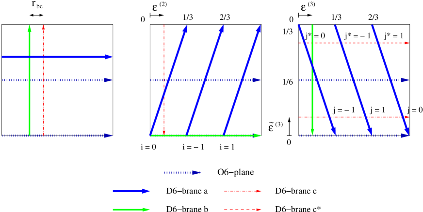
Figure 8: Brane configuration corresponding to the MSSM-like model described in the text, for the choice $\rho=1$. For simplicity, we have not depicted the leptonic stack nor the mirror $a$* stack.

Considering the leptonic sector involves triplets $dbc$ and $dbc$*. Now, since the stack $d$ is similar to the $a$, the above discussion also apply to this case, and the only change that we have to make is considering new variables $(\epsilon^{(2)}_{l},\epsilon^{(3)}_{l};\theta^{(2)}_{l},\theta^{(3)}_{l})$ instead of $(\epsilon^{(2)},\epsilon^{(3)};\theta^{(2)},\theta^{(3)})$. Notice that the difference of this two sets of variables parametrizes the breaking $SU(4)\rightarrow SU(3)\times U(1)_{B-L}$, whereas $(\epsilon_{c}^{(3)},\theta_{c}^{(3)})$ parametrize $SU(2)_{R}\rightarrow U(1)_{c}$ breaking.

On the other hand, Yukawa couplings depend only on two closed string parameters, namely the complex Kähler structures on the second and third tori, through $\kappa^{(r)}=3J^{(r)}/\alpha^{\prime}=3\chi(R^{(r)})^{2}/\alpha^{\prime}$, $r=2,3$. Since the index $i$ is an index labeling left-handed quarks, whereas $j$, $j$* label up-like and down-like right-handed quarks, our Yukawa couplings will be of the form

$$Y_{ij}^{U}Q_{L}^{i}H_{u}U_{R}^{j},\quad\quad Y_{ij*}^{D}Q_{L}^{i}H_{d}D_{R}^{j*},$$ (84)

with Yukawa matrices

$$\begin{array}[]{c}Y_{ij}^{U}\sim\vartheta\left[\begin{array}[]{c}\frac{i}{3}+\epsilon^{(2)}\\ \theta^{(2)}\end{array}\right]\left({3J^{(2)}\over\alpha^{\prime}}\right)\times\vartheta\left[\begin{array}[]{c}\frac{j}{3}+\epsilon^{(3)}+\tilde{\epsilon}^{(3)}\\ \theta^{(3)}+\tilde{\theta}^{(3)}\end{array}\right]\left({3J^{(3)}\over\alpha^{\prime}}\right),\\ Y_{ij*}^{D}\sim\vartheta\left[\begin{array}[]{c}\frac{i}{3}+\epsilon^{(2)}\\ \theta^{(2)}\end{array}\right]\left({3J^{(2)}\over\alpha^{\prime}}\right)\times\vartheta\left[\begin{array}[]{c}\frac{j*}{3}+\epsilon^{(3)}-\tilde{\epsilon}^{(3)}\\ \theta^{(3)}-\tilde{\theta}^{(3)}\end{array}\right]\left({3J^{(3)}\over\alpha^{\prime}}\right).\end{array}$$ (85)

We can apply analogous arguments for the case $\rho=1/3$ in table 3. The final result is

$$Y_{ij}^{U}\sim\vartheta\left[\begin{array}[]{c}\frac{j}{3}+\epsilon^{(2)}\\ \theta^{(2)}\end{array}\right]\left({3J^{(2)}\over\alpha^{\prime}}\right)\times\vartheta\left[\begin{array}[]{c}\frac{i}{3}+\epsilon^{(3)}+\tilde{\epsilon}^{(3)}\\ \theta^{(3)}+\tilde{\theta}^{(3)}\end{array}\right]\left({3J^{(3)}\over\alpha^{\prime}}\right)$$ (86)

for the up-like couplings, whereas the down-like ones are obtained form (86) by the replacement $(\epsilon_{c}^{(3)},\theta_{c}^{(3)})\mapsto(-\epsilon_{c}^{(3)},-\theta_{c}^{(3)})$.

The quark and lepton mass spectrum can be easily computed from these data. Indeed, let us consider the quark mass matrices proportional to (85), and define

$$\begin{array}[]{rcl}a_{i}&\equiv&\vartheta\left[\begin{array}[]{c}\frac{i}{3}+\epsilon^{(2)}\\ \theta^{(2)}\end{array}\right]\left({3J^{(2)}\over\alpha^{\prime}}\right),\\ b_{j}&\equiv&\vartheta\left[\begin{array}[]{c}\frac{j}{3}+\epsilon^{(3)}+\tilde{\epsilon}^{(3)}\\ \theta^{(3)}+\tilde{\theta}^{(3)}\end{array}\right]\left({3J^{(3)}\over\alpha^{\prime}}\right),\\ \tilde{b}_{j*}&\equiv&\vartheta\left[\begin{array}[]{c}\frac{j*}{3}+\epsilon^{(3)}-\tilde{\epsilon}^{(3)}\\ \theta^{(3)}-\tilde{\theta}^{(3)}\end{array}\right]\left({3J^{(3)}\over\alpha^{\prime}}\right).\end{array}$$ (87)

Then, the Yukawa matrices can be expressed as

$$Y^{U}\sim A\cdot\left(\begin{array}[]{ccc}1&1&1\\ 1&1&1\\ 1&1&1\end{array}\right)\cdot B,\quad\quad Y^{D}\sim A\cdot\left(\begin{array}[]{ccc}1&1&1\\ 1&1&1\\ 1&1&1\end{array}\right)\cdot\tilde{B}.$$ (88)

$$\begin{array}[]{ccc}A=\left(\begin{array}[]{ccc}a_{1}&&\\ &a_{0}&\\ &&a_{-1}\end{array}\right)&B=\left(\begin{array}[]{ccc}b_{1}&&\\ &b_{0}&\\ &&b_{-1}\end{array}\right)&\tilde{B}=\left(\begin{array}[]{ccc}\tilde{b}_{1}&&\\ &\tilde{b}_{0}&\\ &&\tilde{b}_{-1}\end{array}\right).\end{array}$$ (89)

In order to compute the mass eigenstates, we can consider the hermitian, definite positive matrix $Y\cdot Y^{\dagger}$ and diagonalize it. Let us take, for instance, $Y^{U}$. We find

$$Y^{U}\cdot(Y^{U})^{\dagger}\sim{\rm Tr\,}(B\cdot\bar{B})\quad A\cdot\left(\begin{array}[]{ccc}1&1&1\\ 1&1&1\\ 1&1&1\end{array}\right)\cdot\bar{A},$$ (90)

where bar denotes complex conjugation. This matrix has one nonzero eigenvalue given by

$$\lambda^{U}={\rm Tr\,}(A\cdot\bar{A})\ {\rm Tr\,}(B\cdot\bar{B}), |\lambda^{U}\rangle={A\over\sqrt{{\rm Tr\,}(A\cdot\bar{A})}}\cdot\left(\begin{array}[]{c}1\\ 1\\ 1\end{array}\right),$$ (94)

and two zero eigenvalues whose eigenvectors span the subspace

$$\bar{A}^{-1}\cdot\left[{\rm Ker}\left(\begin{array}[]{ccc}1&1&1\\ 1&1&1\\ 1&1&1\end{array}\right)\right]\bigcup{\rm Ker}\bar{A}.$$ (95)

Similar considerations can be applied to $Y^{D}$, and the results only differ by the replacement $B\rightarrow\tilde{B}$. This provides a natural mass scale between up-like and down-like quarks:

$${m_{U}\over m_{D}}\sim\sqrt{\frac{{\rm Tr\,}(B\cdot\bar{B})}{{\rm Tr\,}(\tilde{B}\cdot\bar{\tilde{B}})}}$$ (96)

(we should also include $\langle H_{u}\rangle/\langle H_{d}\rangle$ in order to connect with actual quark masses). This ratio is equal to one whenever $\tilde{\epsilon}^{(3)}=-\tilde{\epsilon}^{(3)}\ {\rm mod}\ 1/3$ and $\tilde{\theta}^{(3)}=-\tilde{\theta}^{(3)}\ {\rm mod}\ 1$. These points in moduli space correspond precisely to the enhancement $U(1)_{c}\rightarrow SU(2)_{R}$, where we would expect equal masses for up-like and down-like quarks. On the other hand, we find that the CKM matrix is the identity at every point in the moduli space.

Thus we find that in this simple model only the third generation of quarks and leptons are massive. This could be considered as a promising starting point for a phenomenological description of the SM fermion mass spectrum. One can conceive that small perturbations of this simple brane setup can give rise to smaller but non-vanishing masses for the rest of quarks and leptons as well as non-vanishing CKM mixing . We postpone a detailed study of Yukawa couplings in semirealistic intersecting D-brane models to future work.

The previous discussion parallels for the case $\rho=1/3$. Indeed, we find the same mass spectrum of two massless and one massive eigenvalue for each Yukawa matrix. The only difference arises from the CKM matrix, which is not always the identity but only for the special values of $(\tilde{\epsilon}^{(3)},\tilde{\theta}^{(3)})$ where the symmetry enhancement to $SU(2)_{R}$ occurs.

5 Extension to elliptic fibrations

Although so far we have concentrated on computing Yukawa couplings in toroidal compactifications, it turns out that the same machinery can be applied to certain D-brane models involving non-trivial Calabi-Yau geometries. Indeed, in [17] a whole family of intersecting D6-brane models wrapping 3-cycles of non-compact ${\bf CY_{3}}$’s was constructed. The simplest of such local Calabi-Yau geometries was based on elliptic and ${\bf C}$* fibrations over a complex plane, parametrized by $z$. In this setup, gauge theories arise from D6-branes wrapping compact special Lagrangian 3-cycles which, roughly speaking, consist of real segments in the complex $z$-plane over which two $S^{1}$ are fibered. One of such $S^{1}$ is a non-contractible cycle in ${\bf C}$*, while the other wraps a $(p,q)$ 1-cycle on the elliptic fiber. The intersection of any such compact 3-cycles is localized on the base point $z=0$, where the ${\bf C}$* fibre degenerates to ${\bf C}\times{\bf C}$. We refer the reader to [17, 53] for details on this construction.

The important point for our discussion is that the geometry of any number of intersecting D6-branes can be locally reduced to that of intersecting 1-cycles on the elliptic fiber in $z=0$, that is, to that of $(p_{\alpha},q_{\alpha})$ cycles on a $T^{2}$. Moreover, due to this local geometry, any worldsheet instanton connecting a triplet of D6-branes will also be localized in the elliptic fiber at $z=0$. The computation of Yukawas in this ${\bf CY_{3}}$ setup then mimics the one studied in section 3.1, where we considered worldsheet instantons on a $T^{2}$.

As a result, we find that the structure of Yukawa couplings computed in section 3, which could be expressed in terms of (multi) theta functions, is in fact more general than the simple case of factorizable cycles in a $T^{2n}$. In fact, it turns out to be even more general than intersecting brane worlds setup. Indeed, as noticed in [17], this family of non-compact ${\bf CY_{3}}$ geometries is related, via mirror symmetry, to Calabi-Yau threefold singularities given by complex cones over del Pezzo surfaces. In turn, the intersecting D6-brane content corresponds to D3-branes sitting on such singularities.

Let us illustrate these facts with a simple example already discussed in [17], section 2.5.1. The brane content consist of three stacks of $N$ branes each, wrapping the 1-cycles

$$\Pi_{a}=(2,-1),\quad\Pi_{b}=(-1,2),\quad\Pi_{c}=(-1,-1),$$ (97)

with intersection numbers $I_{ab}=I_{bc}=I_{ca}=3$. This yields a simple ${\cal N}=1$ spectrum with gauge group $U(N)^{3}$ and matter triplication in each bifundamental. We have depicted the D-brane content of (97) in figure 9, restricting ourselves to the elliptic fiber on the base point $z=0$. Notice that the complex structure of such $T^{2}$ is fixed by the ${\bf Z}_{3}$ symmetry that the whole configuration must preserve [17].

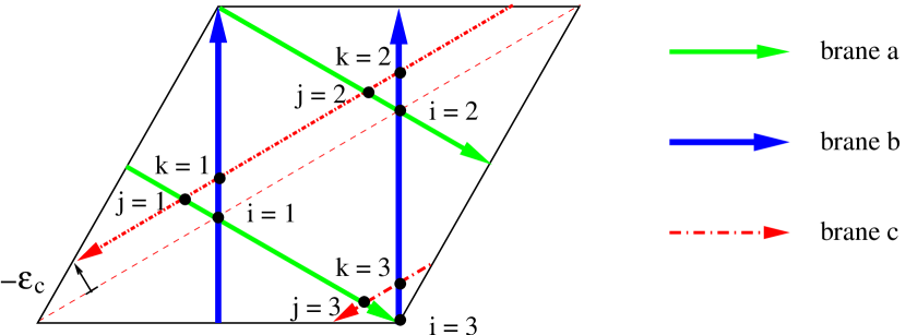
Figure 9: D-brane configuration in (97), restricted to the elliptic fibre at $z=0$ in the base space. Due to the quantum ${\bf Z}_{3}$ symmetry of this configuration, each stack of branes must be related to the others by a $e^{\pm 2\pi i/3}$ rotation. Hence, the complex structure of the elliptic fibre is frozen. Notice that a triangle between vertices $i$, $j$, $k$ closes only if the condition $i+j+k\equiv 0$ mod $3$ is satisfied.

Notice also that the intersection numbers are not coprime, so the Yukawa couplings between intersections $i$, $j$, $k$ will be given by a theta function with characteristics (44), (45) and (46), with $d=3$. Given the specific choice of numbering of figure 9, we can take the linear function $s$ to be $s=-k-2j$. Moreover, not all the triplet of intersections are connected by an instanton, but they have to satisfy the selection rule

$$i+j+k\equiv 0\ {\rm mod}\ 3.$$ (98)

This give us the following form for the Yukawa couplings in the present model

$$Y_{ij1}\sim\left(\begin{array}[]{ccc}A&0&0\\ 0&0&B\\ 0&C&0\end{array}\right),\quad Y_{ij2}\sim\left(\begin{array}[]{ccc}0&0&C\\ 0&A&0\\ B&0&0\end{array}\right),\quad Y_{ij3}\sim\left(\begin{array}[]{ccc}0&B&0\\ C&0&0\\ 0&0&A\end{array}\right),$$ (99)

with

$$A=\vartheta\left[\begin{array}[]{c}\epsilon/3\\ 3\theta\end{array}\right](3J/\alpha^{\prime}),\quad B=\vartheta\left[\begin{array}[]{c}(\epsilon-1)/3\\ 3\theta\end{array}\right](3J/\alpha^{\prime}),\quad C=\vartheta\left[\begin{array}[]{c}(\epsilon+1)/3\\ 3\theta\end{array}\right](3J/\alpha^{\prime}),$$ (100)

and where we have defined the parameters $\epsilon=\epsilon_{a}+\epsilon_{b}+\epsilon_{c},\ \theta=\theta_{a}+\theta_{b}+\theta_{c}\in[0,1)$.

A particularity of these elliptically fibered 3-cycles which the D6-branes wrap is that, topologically, they are 3-spheres. This means they are simply connected and, by [36], their moduli space is zero-dimensional. This means that the D-brane position parameter $\epsilon_{\alpha}$ is fixed, and the same story holds for $\theta_{\alpha}$. Although frozen, we do not know the precise value of these quantities and, presumably, different values will correspond to different physics.

This simple model with matter triplication is in fact mirror to the ${\bf C}^{3}/{\bf Z}_{3}$ orbifold singularity and, indeed, the chiral matter content exactly reproduces the one obtained from D3-branes at that singularity, in $N$ copies of the fundamental representation [17]. The superpotential of such mirror configuration is given by

$$W=\sum_{\{abc\}}\epsilon^{ijk}[\Phi_{ab}^{i}\Phi_{bc}^{j}\Phi_{ca}^{k}],$$ (101)

where $\{abc\}$ means that we have to consider all the cyclic orderings. This superpotential implies Yukawa couplings of the form $Y_{ijk}\sim\epsilon^{ijk}$. We see that we can reproduce such result in terms of the general solution (99), only if one of the entries $A$, $B$ or $C$ vanishes. Let us take $C\equiv 0$, which can be obtained by fixing the theta-function parameters to be

$$\epsilon=\frac{1}{2},\quad\quad\theta=\frac{2m+1}{6},\ m\in{\bf Z}.$$ (102)

Is easy to see that this condition also implies that $|A|=|B|$. More precisely,

$$A=Z\cdot e^{2\pi i(m+\frac{1}{2})\frac{1}{6}},\quad\quad B=Z\cdot e^{-2\pi i(m+\frac{1}{2})\frac{1}{6}},\quad\quad Z\in{\bf C}.$$ (103)

Now, if we perform the relabeling

$$\begin{array}[]{cc}i:&1\leftrightarrow 3\\ j:&1\leftrightarrow 2\\ k:&2\leftrightarrow 3\end{array}$$ (104)

(which preserves the condition (98)) we are led to Yukawa couplings of the form

$$Y_{ij1}\sim Z\cdot\left(\begin{array}[]{ccc}0&0&0\\ 0&0&\bar{\omega}\\ 0&\omega&0\end{array}\right),\quad Y_{ij2}\sim Z\cdot\left(\begin{array}[]{ccc}0&0&\omega\\ 0&0&0\\ \bar{\omega}&0&0\end{array}\right),\quad Y_{ij3}\sim Z\cdot\left(\begin{array}[]{ccc}0&\bar{\omega}&0\\ \omega&0&0\\ 0&0&0\end{array}\right),$$ (105)

where $\omega={\rm exp}(2\pi i(m+1/2)\cdot 1/6)$. By taking the choice $m=1$, we obtain $\omega=i$, so that $Y_{ijk}\sim\epsilon^{ijk}$, as was to be expected from (101). There are, however, two other inequivalent choices of $\theta$, given by $m=0,2$. Is easy to check that these two values yield the superpotentials corresponding to the two choices of ${\bf C}^{3}/({\bf Z}_{3}\times{\bf Z}_{3}\times{\bf Z}_{3})$ orbifold singularity with discrete torsion, which have the same chiral spectrum as a plain ${\bf C}^{3}/{\bf Z}_{3}$ orbifold . We present such final configuration in figure 10.

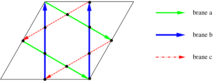
Figure 10: Final D-brane configuration, with the brane positions fixed by (102). Again we restrict to the elliptic fibre at $z=0$ in the base space.

6 Yukawa versus Fukaya

In the previous section we have shown how, combined with mirror symmetry, the computation of worldsheet instantons between chiral fields in intersecting D-brane models can yield a powerful tool to compute Yukawa couplings in more general setups as, e.g., D-branes at singularities. The purpose of the present section is to note that computation of Yukawas and other disc worldsheet instantons is not only a tool, but lies at the very heart of the definition of mirror symmetry. The precise context to look at is Kontsevich’s homological mirror symmetry conjecture [54], performed before the importance of D-branes was appreciated by the physics community. This proposal relates two a priori very different constructions in two different $n$-fold Calabi-Yau manifolds ${\cal M}$ and ${\cal W}$, which are dual (or mirror) to each other. ${\cal M}$ is to be seen as a $2n$-dimensional symplectic manifold with vanishing first Chern class, while ${\cal W}$ shall be regarded as an $n$-dimensional complex algebraic manifold. From the physics viewpoint these are the so-called A-side and B-side of the mirror map, respectively. The structure of complex manifold allows us to construct the derived category of coherent sheaves from ${\cal W}$, which classifies the boundary conditions in the B-twisted topological open string theory model on such manifold, hence the spectrum of BPS branes on the B-side [55]. On the other hand, the symplectic structure on ${\cal M}$ naturally leads to the construction of Fukaya’s category. Kontsevich’s proposal amounts to the equivalence of both categories.

Intersecting D6-brane configurations as described in section 2 lie on the A-side of this story. Hence, they should be described by Fukaya’s category. This seems indeed to be the case and, in the following, we will try to describe the physical meaning of Fukaya’s mathematical construction from the point of view of intersecting D-brane models, paying special attention to the rôle of worldsheet instantons.

Roughly speaking, a category is given by a set of objects and morphisms between them. The objects of the category we want to construct are pairs of the form ${\cal L}_{\alpha}=(\Pi_{\alpha},{\cal E}_{\alpha})$, of special Lagrangian submanifolds $\Pi_{\alpha}$ of ${\cal M}$, endowed with unitary local systems ${\cal E}_{\alpha}$, or flat $U(N_{\alpha})$ gauge bundles. This is precisely the set of objects used as building blocks in our ${\bf CY_{n}}$ intersecting brane configurations, each object associated to a stack of $N_{\alpha}$ D-branes . The morphisms between a pair of objects are generated by the points of intersection of the two sL submanifolds, more precisely

$$Hom({\cal L}_{\alpha},{\cal L}_{\beta})={\#(\Pi_{\alpha}\cap\Pi_{\beta})}\otimes Hom({\cal E}_{\alpha},{\cal E}_{\beta}),$$ (106)

where $Hom({\cal E}_{\alpha},{\cal E}_{\beta})$ represents a morphism of gauge bundles. The morphisms between two objects, then, are naturally associated to the set of chiral fields living at the intersections of two D-branes, which transform under the bifundamental representation of the corresponding gauge groups.

Actually, (106) can be converted to a graded set of morphisms. That is, each intersection $p$ can be attached with an index $\eta(p)\in{\bf Z}$, named Maslov index. The physical meaning of such index is related to how one must describe the spectrum of particles at the intersections from the underlying CFT viewpoint, i.e., two sets of fields arising from two elements of $\Pi_{\alpha}\cap\Pi_{\beta}$ may look locally similar, but related by some spectral flow that the global theory must take into account. In the case of Lagrangian tori, i.e., factorizable D-branes, in $T^{2n}$ all the intersections have the same Maslov index, which can be defined as [56]

$$\eta(p)_{\alpha\beta}=\sum_{r=1}^{n}[\theta_{\alpha\beta}^{r}],$$ (107)

where $[\theta_{\alpha\beta}^{r}]$ is (the integer part of) the angle between $\Pi_{\alpha}$ and $\Pi_{\beta}$ on the $r^{th}$ two-torus, measured in the counterclockwise sense and in units of $\pi$. A quick look at the case $n=3$ (D6-branes) reveals that $\eta(p)$ mod $2$ can be associated to the chirality of the corresponding field at the intersection $p$. In fact, this grading was already present from the very beginning since, actually, (106) is only valid whenever $\Pi_{\alpha}$ and $\Pi_{\beta}$ intersect transversally in ${\cal M}$. In case their intersection is not a point, we should replace (106) by the cohomology complex $H^{*}(\Pi_{\alpha}\cap\Pi_{\beta},Hom({\cal E}_{\alpha},{\cal E}_{\beta}))$, with its associate grading. We finally find that the morphisms of our construction are given by the graded set

$$Hom^{i}({\cal L}_{\alpha},{\cal L}_{\beta})\simeq\bigotimes_{p\in\Pi_{\alpha}\cap\Pi_{\beta}}H^{i-\eta(p)}(\Pi_{\alpha}\cap\Pi_{\beta},Hom({\cal E}_{\alpha},{\cal E}_{\beta})).$$ (108)

In general, categories not only consist of objects and morphisms between them, but also of compositions of morphisms. In [57] Fukaya proved that, actually, an involved structure can be defined in the previous described category. This structure is based on the properties of an $A^{\infty}$ algebra, which is a generalization of a differential graded algebra, and makes Fukaya’s category into an $A^{\infty}$ category. The definition of such category involves

• A class of objects

• For any two objects $X$, $Y$ a Z-graded Abelian group of morphisms $Hom(X,Y)$

• Composition maps

  $$m_{k}:Hom(X_{1},X_{2})\otimes Hom(X_{2},X_{3})\dots\otimes Hom(X_{k},X_{k+1})\rightarrow Hom(X_{1},X_{k+1}),$$

  of degree $2-k$ for all $k\geq 1$, satisfying the $n^{th}$ order associativity conditions

  $\sum_{r,s}(-1)^{\epsilon}m_{n-r+1}(a_{1}\otimes\dots\otimes a_{s-1}\otimes m_{r}(a_{s}\otimes\dots\otimes a_{s+r-1})\otimes a_{s+r}\otimes\dots\otimes a_{n})=0$

  for all $n\geq 1$. Here $\epsilon=(s+1)k+s\left(n+\sum_{j=1}^{s-1}{\rm deg}(a_{j})\right)$.

Notice that the associative condition for $n=1$ reduces to $m_{1}$ being a degree one operator $m_{1}:Hom(X,Y)\rightarrow Hom(X,Y)$ such that $m_{1}\circ m_{1}=0$, hence it defines a coboundary operator which makes $Hom(X,Y)$ a cochain complex (e.g., just as the exterior derivative in the deRham complex). Furthermore, the second relation ($n=2$) means that $m_{2}:Hom(X,Y)\times Hom(Y,Z)\rightarrow Hom(X,Z)$ is a cochain homomorphism, which induces a product on cohomology groups (e.g., analogous to a wedge product in deRham cohomology).

Up to now we have described the two first items of the previous definition, and is in the third one where worldsheet instantons will play a rôle. Indeed, the composition maps $m_{k}$ are constructed by considering holomorphic maps $\phi:D\rightarrow{\cal M}$, taking the boundary of $D$ to $k+1$ Lagrangian submanifolds ${\cal L}_{\alpha}$ in ${\cal M}$ and $k+1$ marked points $z_{\alpha}$ in the cyclic order of $\partial D$ to the intersection points $p_{\alpha}\in\Pi_{\alpha}\cap\Pi_{\alpha+1}$ (see figure 3 for the case $k=2$). Two of these maps are regarded as equivalent if related by a disc conformal automorphism $Aut(D)\simeq PSL(2,{\bf R})$. This is precisely the definition of a euclidean worldsheet connecting $k+1$ fields at the intersection of $k+1$ D-branes and satisfying the classical equations of motion. Let us fix $k+1$ intersections $p_{\alpha}\in\Pi_{\alpha}\cap\Pi_{\alpha+1}$, and the corresponding $k+1$ matrices $t_{\alpha}\in Hom({\cal E}_{\alpha}|_{p_{\alpha}},{\cal E}_{\alpha+1}|_{p_{\alpha+1}})$. If we choose them to have the appropriate degree, the moduli space of holomorphic inequivalent maps connecting them will be discrete, so we can sum over all of such $\phi$ to obtain the quantity

$$C((p_{1},t_{1}),\dots,(p_{k},t_{k}),p_{k+1})=\sum_{\phi}\pm\ e^{2\pi i\int_{\phi(D)}\omega}\ Pe^{\oint_{\phi(\partial D)}\beta},$$ (109)

where the $\pm$ sign stands for holomorphic and antiholomorphic maps, respectively and $\omega$ is the complexified Kähler form in ${\cal M}$. Finally, $P$ stands for a path-ordered integration on the boundary of the disc, with $\beta$ is being the connection of the flat bundles along the boundaries in ${\cal L}_{\alpha}$’s, and the matrices $t_{i}$ inserted at the boundary marked points [58]. The r.h.s. of (109) is thus a homomorphism of ${\cal E}_{1}$ to ${\cal E}_{k+1}$, and we can define the composition maps $m_{k}$ as

$$m_{k}((p_{1},t_{1}),\dots,(p_{k},t_{k}))=\sum_{p_{k+1}\in\Pi_{1}\cap\Pi_{k+1}}C((p_{1},t_{1}),\dots,(p_{k},t_{k}),p_{k+1})\cdot p_{k+1}.$$ (110)

From these definitions, is easy to see that the computation of the composition maps $m_{k}$ is equivalent to computing the worldsheet instanton correction to the superpotential involving $k+1$ chiral fields at the D-branes intersections. Indeed, (109) is nothing but a generalization of (5) for $k+1$ disc insertions. In the case $k=1$, we are evaluating the instantons connecting two chiral fields at the intersections of the same pair of D-branes ${\cal L}_{1}$, ${\cal L}_{2}$, just as in figure 4 (2). Notice that $m_{1}$ has degree $1$, so it can be regarded as a chirality-changing operator, i.e., a mass term. If we consider D-brane configurations consisting of Lagrangian $n$-tori on $T^{2n}$ its action is trivial, $m_{1}\equiv 0$, but this will not be the case in general. Computing the cohomology

$${\{{\rm Ker}\left(m_{1}:Hom^{i}({\cal L}_{\alpha},{\cal L}_{\beta})\rightarrow Hom^{i+1}({\cal L}_{\alpha},{\cal L}_{\beta})\right)\}\over\{{\rm Im}\left(m_{1}:Hom^{i-1}({\cal L}_{\alpha},{\cal L}_{\beta})\rightarrow Hom^{i}({\cal L}_{\alpha},{\cal L}_{\beta})\right)\}},$$ (111)

is equivalent to computing the massless fields in our D-brane configuration. On the other hand, the case $k=2$ coincides with the general computation of Yukawa couplings between chiral fields at sL’s intersections described in section 2.3. Indeed, the action of $m_{2}$ involves three objects of our configurations, hence three D-branes $(a,b,c)$, and three different morphisms between them, hence a triplet of intersections $(i,j,k)$. For each such choice we can define an element of the form (109), which represents a Yukawa coupling. Indeed, in the phenomenological setup of figure 3, if we let $i,j$ index left- and right-handed quarks, respectively, the matrix of maps $(M_{2})_{ij}=m_{2}((p_{i},t_{i}),(p_{j},t_{j}))$ is equivalent to the Yukawa matrix of such chiral fields. In the same manner, the composition maps $m_{k}$, $k\geq 3$ encode the corrections to the superpotential involving non-renormalizable higher dimensional couplings.

$A^{\infty}$ category	Fukaya Category	Intersecting D-branes
Objects	special Lagrangian submanifolds $\Pi_{\alpha}$	D-brane stacks
	endowed with unitary systems ${\cal E}_{\alpha}$	with flat gauge bundles
Morphisms	$Hom({\cal E}_{\alpha},{\cal E}_{\beta})$ generated by	Chiral matter in bifundamentals
	intersection points $p_{\alpha\beta}\in\Pi_{\alpha}\cap\Pi_{\beta}$	localized at the intersections
Grading	Maslov index $\eta(p_{\alpha\beta})$	Spectral flow index
		(mod $2$ $=$ chirality)
Composition maps	Holomorphic discs	Worldsheet instanton corrections
	$m_{1}$	mass operator
	$m_{2}$	Yukawa coupling
	$m_{k}$, $k\geq 3$	non-renormalizable couplings
		involving $k+1$ chiral fields

Table 5: Fukaya-Yukawa dictionary.

We have summarized in table 5 the physical interpretation of the basic quantities conforming Fukaya’s category. This list is not meant to be complete. In fact, it turns out that Fukaya’s categories are not always well defined, and not until very recently has a complete definition of such construction been provided [59]. The computation of such category in the simplest case of a Calabi-Yau one-fold, i.e., the elliptic curve, was performed in [58], where the match with the derived category of coherent sheaves in a T-dual torus was also performed, proving Kontsevich’s conjecture in this case. The extension to higher-dimensional symplectic tori followed in [56]. The similarities of the results in those papers with the computations of section 3 are not an accident, but a sample of the deep mathematical meaning of the computation of Yukawa couplings in intersecting D-brane models.

7 Final comments and conclusions

In the present paper we have addressed the computation of Yukawa couplings among chiral fields living at the intersections of wrapping D-branes. The simplest class of models considered are toroidal (orientifold) compactifications of Type IIA string theory with D6-branes wrapping factorizable 3-cycles on $T^{2}\times T^{2}\times T^{2}$. The Yukawa couplings come from holomorphic world-sheet instanton contributions. We find that the Yukawa couplings have simple expressions in terms of (products) of complex Jacobi theta functions with characteristics. They depend on the Kähler class of the tori and on the open string moduli but not on the complex structure. They do not depend explicitly on the particular wrapping numbers of the D6-branes but rather on the intersection numbers on the different subtori.

This class of toroidal models are of phenomenological interest since one can find specific D-brane configurations with the chiral spectrum of the SM living at the intersections. We provide an specific example in which the massless chiral spectrum is that of the minimal supersymmetric standard model and compute the corresponding physical Yukawa couplings. They have a simple expression in terms of a product of two complex theta functions depending on the Kähler class and the open string moduli. In this simple model only one generation of quarks and leptons get mass and the other two are massless. This may be considered a satisfactory starting point for a fully successful description of the observed spectrum of quarks and leptons since small deviations of the simple configuration considered could give rise to smaller masses for the rest of the generations. A more complete study of the structure of Yukawa couplings in intersecting D-brane models is of clear interest and is at present underway [60].

The methods we employed for the computation of Yukawa couplings may also be applied to more general manifolds. In particular we have shown how one can compute the Yukawa couplings in certain classes of elliptically fibered CY manifolds which are mirror to D3-branes sitting on complex cones over del Pezzo surfaces. We compute the Yukawa couplings on a particular simple manifold which is known to be mirror to D3-branes sitting on a ${{\bf C}^{3}}/{\bf Z}_{3}$ singularity and show that they match with the known Yukawa couplings in the mirror theory. Similarly, one could foresee computing Yukawa couplings of more complicated models involving other del Pezzo surfaces, as well as those models which involve D-branes with magnetic fluxes on Type IIB or Type I toroidal compactifications [2, 61]. The latter are related with our intersecting D-brane configurations of section 3 by plain toroidal T-duality [1, 62].

We have found a connection between Yukawa couplings in D6-brane intersecting brane setups of Type IIA string theory and Fukaya’s category in a symplectic manifold. We provide a dictionary giving the mathematical concept associated to each of the physical objects. It would be very interesting to pursue this connection further and provide a more detailed dictionary.

In summary, we have shown how the computation of Yukawa couplings in intersecting D-brane configurations offers an interesting point of connection of very phenomenological questions like the structure of quark and lepton masses and very abstract mathematical notions like that of Fukaya’s category. We find amusing that, after all, the work of Yukawa could be connected to that of Fukaya!

Acknowledgments

We are grateful to G. Aldazábal, F. Quevedo, R. Rabadán and A. Uranga for very useful comments and discussions. L.E.I and F.M. thank CERN’s Theory Division were part of this work was carried out. The research of D.C. and F.M. was supported by the Ministerio de Educación, Cultura y Deporte (Spain) through FPU grants. This work is partially supported by CICYT (Spain) and the European Commission (RTN contract HPRN-CT-2000-00148).

Appendix A Higher dimensional holomorphic discs

The aim of this section is to show the existence and uniqueness of (anti)holomorphic worldsheet instantons that connect factorizable $n$-cycles in $T^{2n}$. Contrary to Euclidean intuition, these volume-minimizing surfaces are not, in general, given by flat triangles of ${\bf R}^{2n}$ but by more complicated calibrated manifolds.

Let us first describe the problem more precisely. For simplicity, instead of dealing with the complex manifold $T^{2}\times\dots\times T^{2}$ equipped with a complex structure, let us consider its covering space, given by ${\bf C}^{n}$. The factorizable $n$-cycles of (51) are mapped to affine Lagrangian $n$-planes given by

$$L_{\alpha}=\bigotimes_{r=1}^{n}\{t^{(r)}\cdot z_{\alpha}^{(r)}+v_{\alpha}^{(r)}|t^{(r)}\in{\bf R}\},$$ (112)

where the fixed quantities $z_{\alpha}^{(r)},v_{\alpha}^{(r)}\in{\bf C}$ define the affine equation of a line in the $r^{th}$ complex plane. Of course, we should also consider all the copies of such affine subspace under $T^{2n}$ lattice translations, which implies the modification $v_{\alpha}^{(r)}\mapsto v_{\alpha}^{(r)}+l_{1}^{(r)}+\tau^{(r)}l_{2}^{(r)}$, $l_{1}^{(r)},l_{2}^{(r)}\in{\bf Z}$ in (112) (see figure 5 for an example of this). For our purposes, however, it will suffice to consider just a single copy given by (112).

Let us now consider a triplet of such $n$-hyperplanes $(L_{a},L_{b},L_{c})$ in ${\bf C}^{n}$. Two by two, these hyperplanes will either intersect at a single point in ${\bf C}^{n}$ either be parallel in $s$ complex dimensions. If that is the case, we will consider that they are on top on each other on such complex dimensions, intersecting in a Lagrangian hyperplane of real dimension $s<n$. We can visualize such geometry by projecting it into each complex dimension ${\bf C}_{(r)}$. This picture will look as three real lines $l_{a}^{(r)},l_{b}^{(r)},l_{c}^{(r)}\subset{\bf C}_{(r)}$ forming a triangle whose vertices are the projection of the hyperplanes’ intersections. If two hyperplanes are parallel in such complex dimension, the corresponding triangle will be degenerate (see figure 11).

A worldsheet instanton will be described by a map $\varphi:D\rightarrow{\bf C}^{n}$ with the following properties:

• $\varphi$ is either holomorphic or antiholomorphic.

• $\varphi(\omega_{ab})=L_{a}\cap L_{b}$, $\varphi(\omega_{bc})=L_{b}\cap L_{c}$, $\varphi(\omega_{ca})=L_{c}\cap L_{a}$, where $\omega_{ab},\omega_{bc},\omega_{ca}\in\partial D$ are counterclockwise ordered in $\partial D$.

• $\varphi(\partial D_{a})\subset L_{a}$,  $\varphi(\partial D_{b})\subset L_{b}$,  $\varphi(\partial D_{c})\subset L_{c}$, where $\phi(\partial D_{a})$ is the part of $\partial D$ between $\omega_{ca}$ and $\omega_{ab}$, etc.

Furthermore, since we are only interested in the embedded surface $\varphi(D)$, we must quotient our space of solutions by $Aut(D)=PSL(2,{\bf R})$.

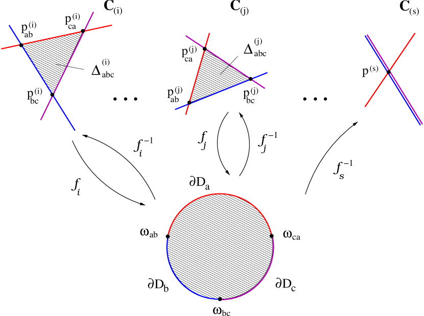
Figure 11: Construction of higher dimensional holomorphic discs.

Let us first focus on the simple case $n=1$, where the worldsheet instanton will have the form of a triangle $\Delta_{abc}\subset{\bf C}$. The Riemmann Mapping Theorem [63] asserts that there exist a one-to-one analytic function $f:{\bf C}\rightarrow D$ such that the image of $Int(\Delta_{abc})$ is $Int(D)$. Moreover, this function is unique up to the group of conformal maps of the open unit disc into itself, which is given by

$${\rm Conf}(D)=\{\phi_{\omega}^{\tau}(z)=\tau\cdot{z-\omega\over 1-\bar{\omega}z}|\omega\in Int(D),\tau\in\partial D\}.$$ (113)

A several statement holding for antianalytic functions. If we also require the boundary of such regions to match under $f$, that is, if we require $f(\partial\Delta_{abc})=\partial D$ following the second point above, then we will select one unique map from the whole family $\phi_{\omega}^{\tau}\circ f$, since Con$(D)\cong PSL(2,{\bf Z})$, and this latter group can be fixed by specifying the location of $\omega_{ab}$, $\omega_{bc}$ and $\omega_{ca}$ in $\partial D$. Moreover, the map $f$ will be either analytic or antianalytic, but not both. Finally, the third point is satisfied by continuity of $f$.

We have thus shown that, for the case $n=1$ there exist a unique function, given by $f^{-1}$, that describes our worldsheet instanton. From this simple result we can derive the statement for general $n$. Indeed, let us consider the $n$ functions $f_{(r)}$ which are obtained from the above construction, now with the triangles $\Delta_{abc}^{(r)}$ which are defined from the lines $l_{a}^{(r)},l_{b}^{(r)},l_{c}^{(r)}\subset{\bf C}_{(r)}$. That is, we consider the same problem for each projection into ${\bf C}_{(r)}$. In case the triangle is degenerate (e.g., $l_{b}^{(s)}=l_{c}^{(s)}$ for some $s$) then such function does not exist, and we take $f^{-1}$ to be the constant map from $D$ to the common intersection point of the three lines. After this, is easy to see that the desired (anti)holomorphic surface is given by $\phi(D)=\vec{f}^{-1}(D)$, where

$$\vec{f}^{-1}(\omega)=\left(f_{1}^{-1}(\omega),f_{2}^{-1}(\omega),\dots,f_{n}^{-1}(\omega)\right)\in{\bf C}^{n},\quad\quad\omega\in D,$$ (114)

and that this surface satisfies all the three requirements above.

A consequence of the holomorphic properties of $\vec{f}$ is that $S=\phi(D)$ will be a surface calibrated by the Kähler 2-form. It is natural to wonder which is the ’shape’ of $S$ in terms of ${\bf C}^{n}$ geometry. A naïve guess would lead us to think that, being surface minimizing, it has a triangular shape. This will not, however, be the generic case. Indeed, let us consider the relatively simple case of two-complex dimensions. In this case, $\vec{f}^{-1}=\left(f_{1}^{-1},f_{2}^{-1}\right)$ maps $D$ into $\Delta_{abc}^{1}\times\Delta_{abc}^{2}\subset{\bf C}^{2}$. We can see the surface $\vec{f}^{-1}(D)$ embedded on ${\bf C}^{2}$ by considering the graph

$$(z_{1},z_{2})=(z_{1},f_{2}^{-1}\circ f_{1}(z_{1})),\quad z_{1}\in\Delta_{abc}^{1}.$$ (115)

Clearly, $f_{2}^{-1}\circ f_{1}(\Delta_{abc}^{1})=\Delta_{abc}^{2}$. This surface will be a triangle in ${\bf C}^{2}$ only if $f_{2}^{-1}\circ f_{1}$ is a constant complex number, that is, only if $\Delta_{abc}^{1}$ and $\Delta_{abc}^{2}$ are congruent triangles. A similar argument can be carried out for higher dimensions.

References

- [1] M. Berkooz, M. R. Douglas and R. G. Leigh, “Branes intersecting at angles,” Nucl. Phys. B 480, 265 (1996), hep-th/9606139.
- [2] R. Blumenhagen, L. Görlich, B. Körs and D. Lüst, “Noncommutative compactifications of type I strings on tori with magnetic background flux,” JHEP 0010, 006 (2000), hep-th/0007024.
- [3] G. Aldazábal, S. Franco, L. E. Ibáñez, R. Rabadán and A. M. Uranga, “D = 4 chiral string compactifications from intersecting branes,” J. Math. Phys. 42, 3103 (2001), hep-th/0011073.
- [4] G. Aldazábal, S. Franco, L. E. Ibáñez, R. Rabadán and A. M. Uranga, “Intersecting Brane Worlds,” JHEP 0102, 047 (2001), hep-ph/0011132.
- [5] R. Blumenhagen, B. Körs and D. Lüst, “Type I strings with F- and B-flux,” JHEP 0102, 030 (2001), hep-th/0012156.
- [6] L. E. Ibáñez, F. Marchesano and R. Rabadán, “Getting just the Standard Model at Intersecting Branes,” JHEP 0111, 002 (2001), hep-th/0105155.
- [7] R. Blumenhagen, B. Körs, D. Lüst and T. Ott, “The standard model from stable intersecting brane world orbifolds,” Nucl. Phys. B 616, 3 (2001), hep-th/0107138.
- [8] M. Cvetič, G. Shiu and A. M. Uranga, “Three-family supersymmetric standard like models from intersecting branes,” Phys. Rev. Lett. 87, 201801 (2001), hep-th/0107143. “Chiral four-dimensional N = 1 supersymmetric type IIA orientifolds from intersecting branes,” Nucl. Phys. B 615, 3 (2001), hep-th/0107166.
- [9] D. Bailin, G. V. Kraniotis and A. Love, “Standard-like models from intersecting D4-branes,” Phys. Lett. B 530, 202 (2002), hep-th/0108131. “Standard-like models from intersecting D5-branes,” hep-th/0210219.
- [10] G. Honecker, “Intersecting brane world models from D8-branes on type IIA orientifolds,” JHEP 0201, 025 (2002), hep-th/0201037.
- [11] D. Cremades, L. E. Ibáñez and F. Marchesano, “SUSY quivers, intersecting branes and the modest hierarchy problem,” JHEP 0207, 009 (2002), hep-th/0201205.
- [12] D. Cremades, L. E. Ibáñez and F. Marchesano, “Intersecting brane models of particle physics and the Higgs mechanism,” JHEP 0207, 022 (2002), hep-th/0203160.
- [13] C. Kokorelis, “GUT model hierarchies from intersecting branes,” JHEP 0208, 018 (2002), hep-th/0203187. “New standard model vacua from intersecting branes,” JHEP 0209, 029 (2002), hep-th/0205147. “Exact standard model compactifications from intersecting branes,” JHEP 0208, 036 (2002), hep-th/0206108. “Exact standard model structures from intersecting D5-branes,” hep-th/0207234. “Deformed intersecting D6-brane GUTs. I,” JHEP 0211, 027 (2002), hep-th/0209202. “Deformed intersecting D6-brane GUTs. II,” hep-th/0210200. “Deformed intersecting D6-brane GUTs and N = 1 SUSY,” hep-th/0212281.
- [14] D. Cremades, L. E. Ibáñez and F. Marchesano, “Standard model at intersecting D5-branes: Lowering the string scale,” Nucl. Phys. B 643, 93 (2002), hep-th/0205074.
- [15] R. Blumenhagen, V. Braun, B. Körs and D. Lüst, “Orientifolds of K3 and Calabi-Yau manifolds with intersecting D-branes,” JHEP 0207, 026 (2002), hep-th/0206038.
- [16] J. R. Ellis, P. Kanti and D. V. Nanopoulos, “Intersecting branes flip SU(5),” hep-th/0206087.
- [17] A. M. Uranga, “Local models for intersecting brane worlds,” JHEP 0212, 058 (2002), hep-th/0208014.
- [18] R. Blumenhagen, L. Görlich and T. Ott, “Supersymmetric intersecting branes on the type IIA orientifold,” hep-th/0211059.
- [19] M. Cvetič, I. Papadimitriou and G. Shiu, “Supersymmetric three family SU(5) grand unified models from type IIA orientifolds with intersecting D6-branes,” hep-th/0212177.
-
[20]
N. Arkani-Hamed, S. Dimopoulos and G. R. Dvali,
“The hierarchy problem and new dimensions at a
millimeter,”
Phys. Lett. B 429, 263 (1998),
hep-ph/9803315.
I. Antoniadis, N. Arkani-Hamed, S. Dimopoulos and G. R. Dvali, “New dimensions at a millimeter to a Fermi and superstrings at a TeV,” Phys. Lett. B 436, 257 (1998), hep-ph/9804398. - [21] J. García-Bellido, R. Rabadán and F. Zamora, “Inflationary scenarios from branes at angles,” JHEP 0201, 036 (2002), hep-th/0112147.
- [22] R. Blumenhagen, B. Körs, D. Lüst and T. Ott, “Hybrid inflation in intersecting brane worlds,” Nucl. Phys. B 641, 235 (2002), hep-th/0202124.
- [23] N. Jones, H. Stoica and S. H. Tye, “Brane interaction as the origin of inflation,” JHEP 0207, 051 (2002) hep-th/0203163.
- [24] M. Gomez-Reino and I. Zavala, “Recombination of intersecting D-branes and cosmological inflation,” JHEP 0209, 020 (2002), hep-th/0207278.
-
[25]
S. Hamidi and C. Vafa,
“Interactions On Orbifolds,”
Nucl. Phys. B 279, 465 (1987).
L. J. Dixon, D. Friedan, E. J. Martinec and S. H. Shenker, “The Conformal Field Theory Of Orbifolds,” Nucl. Phys. B 282, 13 (1987). - [26] A. M. Uranga, “Chiral four-dimensional string compactifications with intersecting D-branes,” hep-th/0301032.
- [27] A. M. Uranga, “D-brane probes, RR tadpole cancellation and K-theory charge,” Nucl. Phys. B 598, 225 (2001), hep-th/0011048.
- [28] A. Sagnotti, “A Note on the Green-Schwarz mechanism in open string theories,” Phys. Lett. B 294, 196 (1992), hep-th/9210127.
- [29] L.E. Ibáñez, R. Rabadán and A. Uranga, “Anomalous U(1)’s in Type I and Type IIB D=4,N=1 string vacua”, Nucl. Phys. B 542, 112 (1999), hep-th/9808139.
- [30] A. M. Uranga, “D-brane, fluxes and chirality,” JHEP 0204, 016 (2002), hep-th/0201221.
- [31] T. Hübsch, “Calabi-Yau Manifolds: A Bestiary For Physicists,”
- [32] D. Joyce, “Lectures on Calabi-Yau and special Lagrangian geometry,” math.dg/0108088.
- [33] M. R. Douglas, “Topics in D-geometry,” Class. Quant. Grav. 17, 1057 (2000), hep-th/9910170.
- [34] R. Harvey and H. B. Lawson, “Calibrated geometries,” Acta Math. 148, 47 (1982).
- [35] K. Becker, M. Becker and A. Strominger, “Five-branes, membranes and nonperturbative string theory,” Nucl. Phys. B 456, 130 (1995), hep-th/9507158.
- [36] R. C. McLean, “Deformations of Calibrated Submanifolds,” Commun. Anal. Geom. 6, 705 (1998).
- [37] S. Kachru, “Lectures on warped compactifications and stringy brane constructions,” hep-th/0009247.
- [38] M. Dine, N. Seiberg, X. G. Wen and E. Witten, “Nonperturbative Effects On The String World Sheet 1 & 2, ” Nucl. Phys. B 278, 769 (1986). Nucl. Phys. B 289, 319 (1987).
-
[39]
M. Aganagic and C. Vafa,
“Mirror symmetry, D-branes and counting
holomorphic discs,”
hep-th/0012041.
M. Aganagic, A. Klemm and C. Vafa, “Disk instantons, mirror symmetry and the duality web,” Z. Naturforsch. A 57, 1 (2002), hep-th/0105045.
B. Acharya, M. Aganagic, K. Hori and C. Vafa, “Orientifolds, mirror symmetry and superpotentials,” hep-th/0202208. - [40] S. Kachru, S. Katz, A. E. Lawrence and J. McGreevy, “Open string instantons and superpotentials,” Phys. Rev. D 62, 026001 (2000), hep-th/9912151. “Mirror symmetry for open strings,” Phys. Rev. D 62, 126005 (2000), hep-th/0006047.
- [41] I. Brunner, M. R. Douglas, A. E. Lawrence and C. Romelsberger, “D-branes on the quintic,” JHEP 0008, 015 (2000), hep-th/9906200.
- [42] H. Ooguri and C. Vafa, “Knot invariants and topological strings,” Nucl. Phys. B 577, 419 (2000), hep-th/9912123.
-
[43]
L. E. Ibáñez,
“Standard model engineering with intersecting
branes,”
hep-ph/0109082.
R. Blumenhagen, V. Braun, B. Körs and D. Lüst, “The standard model on the quintic,” hep-th/0210083.
D. Cremades, L. E. Ibáñez and F. Marchesano, “More about the standard model at intersecting branes,” hep-ph/0212048. - [44] S. Kachru and J. McGreevy, “Supersymmetric three-cycles and (super)symmetry breaking,” Phys. Rev. D 61, 026001 (2000), hep-th/9908135.
- [45] M. Klein, “Couplings in pseudo-supersymmetry,” Phys. Rev. D 66, 055009 (2002), hep-th/0205300. “Loop-effects in pseudo-supersymmetry,” hep-th/0209206. “Effective Lagrangians in pseudo-supersymmetry,” hep-th/0209207.
- [46] D. Joyce, “On counting special Lagrangian homology 3-spheres,” Contemp. Math. 314, 125 (2002), hep-th/9907013.
- [47] R. Blumenhagen, V. Braun and R. Helling, “Bound states of D(2p)-D0 systems and supersymmetric p-cycles,” Phys. Lett. B 510, 311 (2001) hep-th/0012157.
- [48] A. M. Uranga, “Localized instabilities at conifolds,” hep-th/0204079.
-
[49]
R. Blumenhagen, L. Görlich and B. Körs,
“Supersymmetric orientifolds in 6D with
D-branes at angles,”
Nucl. Phys. B 569, 209 (2000),
hep-th/9908130.
“Supersymmetric 4D orientifolds of type IIA with
D6-branes at angles,”
JHEP 0001, 040 (2000),
hep-th/9912204.
S. Förste, G. Honecker and R. Schreyer, “Supersymmetric orientifolds in 4D with D-branes at angles,” Nucl. Phys. B 593, 127 (2001), hep-th/0008250. - [50] D. M. Ghilencea, L. E. Ibáñez, N. Irges and F. Quevedo, “TeV-scale Z’ bosons from D-branes,” JHEP 0208, 016 (2002), hep-ph/0205083.
- [51] E. G. Gimon and J. Polchinski, “Consistency Conditions for Orientifolds and D-Manifolds,” Phys. Rev. D 54, 1667 (1996), hep-th/9601038.
- [52] M. Berkooz and R. G. Leigh, “A D = 4 N = 1 orbifold of type I strings,” Nucl. Phys. B 483, 187 (1997), hep-th/9605049.
-
[53]
K. Hori, A. Iqbal and C. Vafa,
“D-branes and mirror symmetry,”
hep-th/0005247.
A. Hanany and A. Iqbal, “Quiver theories from D6-branes via mirror symmetry,” JHEP 0204, 009 (2002), hep-th/0108137. - [54] M. Kontsevich, “Homological Algebra of Mirror Symmetry,” Proceedings of the 1994 International Congress of Mathematics I, Birkäuser, Zürich, 1995, p. 120, alg-geom/9411018.
- [55] M. R. Douglas, “D-branes, categories and N = 1 supersymmetry,” J. Math. Phys. 42, 2818 (2001), hep-th/0011017.
- [56] K. Fukaya, “Mirror symmetry of Abelian variety and multi theta functions,” (revised version 2000).
- [57] K. Fukaya, “Morse homotopy category and Floer homologies,” Proc. of the 1993 GARC Workshop in Geometry and Topology, Seoul National University.
- [58] A. Polishchuk and E. Zaslow, “Categorical mirror symmetry: The Elliptic curve,” Adv. Theor. Math. Phys. 2, 443 (1998), math.ag/9801119.
- [59] K. Fukaya, “Floer homology and Mirror symmetry I & II,” preprints.
- [60] D. Cremades, L.E. Ibáñez and F. Marchesano, work in progress. See also “Towards a theory of quark masses, mixings and CP-violation,” hep-ph/0212064, to be revised.
- [61] C. Angelantonj, I. Antoniadis, E. Dudas and A. Sagnotti, “Type-I strings on magnetised orbifolds and brane transmutation,” Phys. Lett. B 489, 223 (2000) hep-th/0007090.
- [62] R. Rabadán, “Branes at angles, torons, stability and supersymmetry,” Nucl. Phys. B 620, 152 (2002), hep-th/0107036.
- [63] J. B. Conway, “Functions of One Complex Variable,” Springer-Verlag (1978) 317 p.