Spectral flow of the Dirac spectrum in intersecting vortices

The spectrum of the Dirac Hamiltonian in the background of crossing vortices is studied. To exploit the index theorem, and in analogy to the lattice the space-time manifold is chosen to be the four-torus ${\mathbb{T}}^{4}$. For sake of simplicity we consider two idealized cases: infinitely fat and thin transversally intersecting vortices. The time-dependent spectrum of the Dirac Hamiltonian is calculated and in particular the influence of the vortex crossing on the quark spectrum is investigated. For the infinitely fat intersecting vortices it is found that zero modes of the four-dimensional Dirac operator can be expressed in terms of those eigenspinors of the Euclidean time-dependent Dirac Hamiltonian, which cross zero energy. For thin intersecting vortices the time gradient of the spectral flow of the Dirac Hamiltonian is steepest at the time at which the vortices cross each other.

PACS: 11.15.-q, 12.38.Aw

Keywords: Yang-Mills theory, center vortices, index theorem, zero modes

1 Introduction

Center vortices offer an appealing picture of confinement [1, 2], for a recent review see [3]. Furthermore, the deconfinement phase transition can be understood as a depercolation transition [4] and the free energy of a center vortex vanishes in the confinement regime [5]. In fact there is mounting evidence that center vortices play an important rôle in the QCD vacuum. Lattice calculations show that when center vortices are removed from the Yang-Mills ensemble the string tension [6] as well as the quark condensate and topological charge [7] are lost. This indicates that confinement, spontaneous breaking of chiral symmetry and the chiral anomaly are all triggered by center vortex configurations in the Yang-Mills vacuum. Furthermore, lattice calculations [8] show that restoration of chiral symmetry occurs at finite temperature exactly at the deconfinement phase transition. We can therefore expect that confinement and spontaneous breaking of chiral symmetry are related phenomena. While the emergence of the confining potential, i.e. the string tension, as well as the appearance of the deconfinement phase transition can be rather easily understood in a random center vortex model in an analytic fashion, the mechanism of spontaneous breaking of chiral symmetry has not been explained in the vortex picture of the QCD vacuum, yet. The general folklore is that spontaneous breaking of chiral symmetry is generated by the quasi-zero modes in topologically non-trivial field configurations, which give rise to a quasi continuous Dirac spectrum with non-zero level density $\rho(0)$ at zero virtuality and, by the Banks Casher relation, to a non-zero quark condensate $<qq>\sim\rho(0)$. In fact these calculations [9] show, that a non-zero level density at zero virtuality occurs in the confinement phase while a finite gap in the Dirac spectrum is found above the critical temperature.

It is therefore clear that the topological properties of center vortices and their manifestation in the quark spectrum will play the key rôle in the understanding of spontaneous breaking of chiral symmetry in the center vortex picture of the QCD vacuum. In $D=4$ space-time dimensions center vortices represent closed surfaces of quantized electromagnetic flux which produce a non-trivial center element for a Wilson loop when they are topologically non-trivially linked to the latter [12]. The topological charge of center vortices is given by their (oriented) intersection number [12, 13, 14]. According to the index theorem a non-zero topological charge implies zero modes of the Dirac operator [15]. In [16] the quark zero modes in transversally intersecting vortex surfaces have been studied. It was found that these modes are localized at the vortex sheets, in particular at their intersection points. In $D=3$ dimensions a center vortex represents generically a time-dependent closed flux loop. In [12] it was shown that the topological charge of generic center vortices can be expressed by the temporal change of their writhing number, and furthermore transversal intersection points in $D=4$ correspond to crossing of vortex lines in $D=3$. Thus vortex crossings carry topological charge and by the index theorem should consequently manifest themselves in the quark spectrum.

In this paper we study the quark spectrum in the background of time-dependent crossing center vortices. In particular we investigate how the crossing of vortices manifests itself in the quark spectrum. This might bring some light on the mechanism of spontaneous breaking of chiral symmetry in the vortex picture, since it is believed that chiral symmetry breaking is tightly related to the topological properties of gauge fields.

Throughout this paper the space-time-manifold is chosen to be the four-torus ${\mathbb{T}}^{4}$. There is a variety of reasons for studying ${\mathbb{T}}^{4}$: first, ${\mathbb{T}}^{4}$ allows to use the Atiyah-Singer index theorem in a stringent fashion and allows for normalizable spinors in the background of integer flux. Second, the torus simulates a periodic arrangement of vortices. This is much closer to a percolated vortex cluster than two isolated vortices in ${\mathbb{R}}^{4}$. Finally, the torus is the space-time manifold that is also used in lattice calculations.

The quark spectrum and its spectral flow in time-dependent background gauge fields have been addressed in several publications before, e.g. [17, 18, 19]. In these papers strict relations between the spectral flow of the Dirac Hamiltonian and topological properties of the corresponding background gauge field have been derived in Minkowski space-time. In [17, 18] the spectral flow was considered on an infinite time interval, where the background gauge field has to become a pure gauge at $t=-\infty$ and $t=+\infty$. In [19] only spherically symmetric gauge fields have been examined, but the derived results are also valid on a finite time interval. In this paper we analyze the spectral flow in the presence of intersecting center vortices on a compact Euclidean space-time manifold. The present paper is a continuation of ref. [16] where the quark zero modes in intersecting center vortex sheets were considered. In the present paper we will not confine ourselves to the quark zero modes but study the spectral flow as function of the Euclidean time for the time-dependent vortex crossings. From studying the spectral flow we hope to get some insight into the mechanism which produces the quasi-continuous spectrum of Dirac states near zero virtuality. As a byproduct we will also establish a strict relation between the quark zero modes and the (time-dependent) eigenfunctions of the Dirac Hamiltonian in the case where the background fields consist of “vortices” with homogeneously spread out magnetic flux.

The organization of the paper is as follows: In the next section we consider the mathematical idealization of infinitely thick transversally intersecting vortices, i.e. we consider “vortices” which are homogeneously distributed over the transversal dimensions, so that they represent homogeneous field configurations of constant electromagnetic flux. We consider two orthogonally homogeneously distributed fluxes, which can be considered as two infinitely thick intersecting vortices, where the intersection “point” is smeared out over the whole universe. Accordingly the topological charge is homogeneously distributed over space-time. We will study then the eigenmodes of the Dirac Hamiltonian as function of the adiabatic time-evolution of the vortex flux assuming that the three-space is given by a three-torus. In section 3 we study the opposite case of thin transversally intersecting vortices assuming that the two intersecting vortices are orthogonal to each other. We study the spectral flow of the quarks in this vortex background. Finally in section 4 we allow the intersecting vortex sheets to be non-orthogonal and calculate again the spectral flow of the quarks. Some concluding remarks are given in section 5.

2 Fermions in homogeneously intersecting “vortex” fields

The topological charge of a gauge field configuration

$$\nu = \frac{1}{32\pi^{2}}\int{\mathrm{tr}}F\tilde{F}$$ (2.1)

consisting of center vortices is located at the intersection points of the vortices [13, 12]. In [12] the evolution in time of the topological charge of crossing center vortex configuration has been studied. It is the aim of this paper to investigate the spectral flow of the Dirac Hamiltonian in the background of crossing vortices.

As space-time manifold we choose the four-torus ${\mathbb{T}}^{4}$. It can be seen as ${\mathbb{R}}^{4}$ modulo the lattice

$${\mathbb{L}}^{4}=\left\{x\in{\mathbb{R}}^{4}\,|\,x=\sum_{\mu}n_{\mu}e_{\mu}\,,\,n_{\mu}\in{\mathbb{Z}}\right\}\,,$$

where $\{e_{\mu}\}\,,\,\mu=1,\ldots,4$ are four orthogonal basis vectors with lengths $L_{\mu}=|e_{\mu}|$.

To demonstrate how the spectral flow emerges for intersecting center vortices we start with the following $SU(2)$ gauge field configuration on the four-torus ${\mathbb{T}}^{4}$

$$A_{1}=-2\pi ix_{2}/(L_{1}L_{2})\tau_{3}\,,\quad A_{2}=0\,,\quad A_{3}=-2\pi ix_{4}/(L_{3}L_{4})\tau_{3}\,,\quad A_{4}=0\,.$$ (2.2)

This gauge potential describes two intersecting “vortices” whose fluxes are spread out over the whole $x_{1}$-$x_{2}$- and $x_{3}$-$x_{4}$-, respectively, planes. Indeed, this configuration has constant non-zero field strength components

$$F_{12}=2\pi i/(L_{1}L_{2})\tau_{3}\,,\,F_{34}=2\pi i/(L_{3}L_{4})\tau_{3}$$ (2.3)

so that their fluxes are given by

$$\int{\mathrm{d}}\Sigma_{12}F_{12} = \int_{0}^{L_{1}}{\mathrm{d}}x_{1}A_{1}(x_{2}=L_{2})=-i2\pi\tau_{3}\,,$$ (2.4)

$$\int{\mathrm{d}}\Sigma_{34}F_{34} = \int_{0}^{L_{3}}{\mathrm{d}}x_{3}A_{3}(x_{4}=L_{4})=-i2\pi\tau_{3}\,,$$ (2.5)

which is twice the flux of a center vortex. The line integrals appearing here represent the only non-vanishing contributions from the Wilson loops encircling the whole $x_{1}$-$x_{2}$- and $x_{3}$-$x_{4}$-plane, respectively, see fig. 2.

Figure 1: Wilson loop encircling the whole $x_{1}$-$x_{2}$-plane.

Figure 2: Illustration of the spectral flow of left and right handed fermions in topologically non-trivial constant background field strength as function of time $\tau$.

We choose the flux of these configurations to be twice the flux of a center vortex since a single center vortex cannot be accommodated by the torus with fermions in the fundamental representation of the gauge group, see the discussion given below eq. (2.9).

Furthermore, the configuration (2.2) carries topological charge $\nu=-2$ which is homogeneously distributed over space-time, i.e. the intersection “point” of these two very fat vortices is smeared out over the whole space-time. The gauge potential (2.2) satisfies the boundary conditions

$$A_{\nu}(x+e_{\mu}) = A_{\nu}^{U_{\mu}}(x)=U_{\mu}(x)A_{\nu}(x)U_{\mu}^{-1}(x)+U_{\mu}(x)\partial_{\nu}U_{\mu}^{-1}(x)\,,$$ (2.7)

where the transition functions $U_{\mu}$ can be chosen as follows:

$$U_{1}=U_{3}={\mathbbm{1}}\,,\quad U_{2}=\exp{(2\pi ix_{1}/L_{1}\tau_{3})}\,,\quad U_{4}=\exp{(2\pi ix_{3}/L_{3}\tau_{3})}\,.$$ (2.8)

In general the transition functions have to fulfill the cocycle condition

$$U_{\nu}(x+e_{\mu})U_{\mu}(x)Z_{\mu\nu}=U_{\mu}(x+e_{\nu})U_{\nu}(x)\,,$$ (2.9)

where $Z_{\mu\nu}$ are elements from the center of the gauge group. Throughout this paper we consider fermions in the fundamental representation of $SU(2)$. This implies that all $Z_{\mu\nu}$ are equal to ${\mathbbm{1}}$, because fermions in the fundamental representation cannot tolerate twisted boundary conditions which imply the presence of a single center vortex. For later use we also note that under a gauge transformation $A_{\mu}\to A_{\mu}^{V}$ the transition functions transform

$$U^{V}_{\mu}(x)=V(x+e_{\mu})U_{\mu}(x)V(x)^{-1}\,.$$ (2.10)

Furthermore, since our gauge configuration (2.2) satisfies the Weyl gauge $A_{4}=0$ its topological charge (2.1) can be expressed in terms of the (in general non-Abelian) Chern-Simons action $S_{\mathrm{C}S}(x_{4})$ as [12]

$$\nu=\int_{0}^{L_{4}}{\mathrm{d}}x_{4}\partial_{4}S_{\mathrm{C}S}(x_{4})\,.$$ (2.11)

For well localized center vortices (representing closed flux loops in $D=3$) the Chern-Simons action is nothing but their writhing number [12]. For the particular gauge potential (2.2) the Chern-Simons action reduces to

$$S_{\mathrm{C}S}(x_{4})=-\frac{1}{4\pi^{2}}\int_{{\mathbb{T}}^{3}}{\mathrm{tr}}(A_{3}F_{12}){\mathrm{d}}^{3}x=-2\frac{x_{4}}{L_{4}}:=-2\tau\,$$ (2.12)

so that eq. (2.11) yields indeed $\nu=-2$ when the vortex evolves from $\tau=0$ to $\tau=1$.

We are interested in the time-evolution of fermions in the intersecting center vortex background described by the gauge potential (2.2). Specifically we want to study the time-evolution of the spectrum of the three dimensional Dirac-Hamiltonian

$$H(\tau)\psi=E(\tau)\psi\,,$$

i.e. the Dirac energies $E(\tau)$ as function of the dimensionless time $\tau$.

The Dirac Hamiltonian of a massless fermion reads

$$H=-\gamma_{4}\gamma_{i}{\mathrm{D}}_{i}=\left(\begin{array}[]{cc}-i\sigma_{i}{\mathrm{D}}_{i}&0\\ 0&i\sigma_{i}{\mathrm{D}}_{i}\end{array}\right)\,,$$ (2.13)

where ${\mathrm{D}}_{i}=\partial_{i}+A_{i}$ is the covariant derivative. Under gauge transformations $A\to A^{V}$ the Dirac spinors in the fundamental representation of $SU(2)$ transform as

$$\psi(x)\to\psi^{V}(x)=V(x)\psi(x)\,.$$ (2.14)

In view of equation (2.7) this implies the following boundary conditions for fermionic fields

$$\psi(x+e_{\mu})=U_{\mu}(x)\psi(x)\,.$$ (2.15)

Because the gauge potential (2.2) and the transition functions (2.8) are purely Abelian the two color components of the fermionic field decouple from each other. Therefore it is sufficient to consider only one of the two color components, i.e. we restrict ourselves to spinors with the lower color component equal zero. To get the desired results for spinors with the opposite color one has to change the sign of the energy and to exchange the upper with the lower color component. If not stated otherwise, in the following we will always consider the upper color component of the Dirac field.

Coming back to the Dirac spectrum one first observes that it is invariant under the shift $\tau\to\tau+1$. This is because the two corresponding gauge potentials are related by the periodic gauge transformation $V=\exp{(-2\pi ix_{3}/L_{3}\tau_{3})}$ which leaves the above introduced transition functions $U_{1/2/3}$ invariant, see eq. (2.10).

Since $H$ commutes with $\gamma_{5}$ the eigenvectors of $H$ can be chosen as eigenvectors of $\gamma_{5}$. Hence the eigenvectors of $H$ carry good chirality. It remains to find the eigenvectors $\bar{\psi}$ of the Dirac operator

$${{{{\mathrm{D}/\hskip 1.99997pt}_{(3)}}}}=i\sigma_{i}{\mathrm{D}}_{i}\,,\,{{{{\mathrm{D}/\hskip 1.99997pt}_{(3)}}}}\bar{\psi}=E\bar{\psi}$$ (2.16)

in three dimensions. Because of the periodicity in the $3$-direction ($U_{3}={\mathbbm{1}}$) one can make the ansatz

$$\bar{\psi}_{n}(x_{1},x_{2},x_{3})=\tilde{\psi}_{n}(x_{1},x_{2})\exp{(-2\pi inx_{3}/L_{3})}\,.$$

Inserting this ansatz into the eigenvalue equation (2.16) the latter reduces to the eigenvalue problem

$$\left({{{{\mathrm{D}/\hskip 1.99997pt}_{(2)}}}}+\bar{E}_{n}\sigma_{3}\right)\tilde{\psi}_{n}=\lambda\tilde{\psi}_{n}\,,\,\bar{E}_{n}=2\pi\frac{\tau+n}{L_{3}}\,,$$ (2.17)

where ${{{{\mathrm{D}/\hskip 1.99997pt}_{(2)}}}}=i\left(\sigma_{1}{\mathrm{D}}_{1}+\sigma_{2}{\mathrm{D}}_{2}\right)$ is the massless Dirac operator in two dimensions. For the gauge potential (2.2) the eigenvectors and eigenvalues of ${{{{\mathrm{D}/\hskip 1.99997pt}_{(2)}}}}$ are known [20]:

$${{{{\mathrm{D}/\hskip 1.99997pt}_{(2)}}}}\tilde{\phi}_{m}=\tilde{E}_{m}\tilde{\phi}_{m}\,,\,\tilde{E}_{m}={{\mathrm{sign}}}(m)\sqrt{\frac{4\pi m}{L_{1}L_{2}}}\,,\,m\in{\mathbb{Z}}\,.$$ (2.18)

According to the index theorem for Abelian gauge fields in $D=2$ dimensions, (for each color component) there is exactly one zero mode of ${{{{\mathrm{D}/\hskip 1.99997pt}_{(2)}}}}$, namely $\tilde{\phi}_{m=0}$. This zero mode is left handed, i.e. only the lower component of this two-spinor is non-zero. Therefore, the two-spinor $\tilde{\psi}_{nm=0}=\tilde{\phi}_{m=0}(x_{1},x_{2})\exp{(-2\pi inx_{3}/L_{3})}$ is eigenvector of ${{{{\mathrm{D}/\hskip 1.99997pt}_{(3)}}}}$ with eigenvalue $-\bar{E}_{n}$, see eq. (2.17). The explicit form of the function $\tilde{\phi}_{m=0}$ is written down in eq. (B.4). For $m\neq 0$ the eigenvectors $\tilde{\psi}_{n}$ (2.17) are given by linear combinations of $\tilde{\phi}_{m}$ and $\tilde{\phi}_{-m}$

$$\tilde{\psi}_{nm}=\alpha_{nm}\tilde{\phi}_{m}+\beta_{nm}\tilde{\phi}_{-m}$$

Putting this ansatz into eq. (2.17) and noting that $\sigma_{3}\tilde{\phi}_{m}=\phi_{-m}$ one gets the following eigenvalue problem for the vector $(\alpha_{nm},\beta_{nm})$:

$$\left(\begin{array}[]{cc}\tilde{E}_{m}&\bar{E}_{n}\\ \bar{E}_{n}&-\tilde{E}_{m}\end{array}\right)\left(\begin{array}[]{c}\alpha_{nm}\\ \beta_{nm}\end{array}\right) = E_{nm}\left(\begin{array}[]{c}\alpha_{nm}\\ \beta_{nm}\end{array}\right)\,.$$ (2.25)

This eigenvalue problem has for fixed $(n,m)$ two solutions:

$$E_{nm} = \pm\sqrt{{\tilde{E}_{m}}^{2}+{\bar{E}_{n}}^{2}}\,,$$ (2.26)

where the sign is given by the sign of $\tilde{E}_{m}$. One of the two solutions corresponds to positive $m\in{\mathbb{Z}}$ and the other to negative $m\in{\mathbb{Z}}$. Therefore we set $E_{nm}=\tilde{E}_{m}\sqrt{1+(\bar{E}_{n}/\tilde{E}_{m})^{2}}\,,\,m\neq 0$. The corresponding coefficients $\alpha_{nm}$ and $\beta_{nm}$ can be calculated from (2.25).

Using the tensor product notation $\tilde{\phi}\otimes\chi_{l}$ for right handed ($l=1$) and left handed ($l=2$) four-spinors

$$\tilde{\phi}\otimes\chi_{1}=\left(\begin{array}[]{c}\tilde{\phi}\\ 0\\ 0\end{array}\right)\,,\quad\tilde{\phi}\otimes\chi_{2}=\left(\begin{array}[]{c}0\\ 0\\ \tilde{\phi}\end{array}\right)\,,$$ (2.27)

the eigenvalues and eigenfunctions of the Dirac Hamiltonian $H$ (2.13) can be written as

$$E_{mnl}=(-1)^{l}\left\{\begin{array}[]{ll}\displaystyle\tilde{E}_{m}\sqrt{1+\frac{4\pi^{2}(n+\tau)^{2}}{L_{3}^{2}{\tilde{E}_{m}}^{2}}}\,,&m\neq 0\\ \displaystyle-\frac{2\pi}{L_{3}}(n+\tau)\,,&m=0\end{array}\right\}\,,$$ (2.28)

$$\psi_{nml} = \left(\alpha_{nm}\tilde{\phi}_{m}+\beta_{nm}\tilde{\phi}_{-m}\right)\otimes\chi_{l}\,e^{(-2\pi inx_{3}/L_{3})}\,,\,m,n\in{\mathbb{Z}}\,,\,m\neq 0\,,\,l=1,2\,,$$ (2.29)

$$\psi_{n0l} = \tilde{\phi}_{0}\otimes\chi_{l}\,e^{(-2\pi inx_{3}/L_{3})}\,,\,n\in{\mathbb{Z}}\,,\,l=1,2\,.$$ (2.30)

Obviously, only the $m=0$ level can cross zero energy. As the time $\tau$ evolves from $\tau=0$ to $\tau=1$ the left handed ($l=2,m=0$) modes show a spectral flow from positive to negative energy and the right handed ($l=1,m=0$) modes from negative to positive energy, and there is a level crossing through zero energy for $n=-\tau$, see fig. 2. The eigenmodes of the lower color component show the opposite behavior.

Semi-classically, one can interpret the spectral flow induced by the time-evolution $\tau\to\tau+1$ as the creation of a (right handed) particle and a (left handed) anti-particle, i.e. the number of right-handed particles increases by $2$. Correspondingly the Chern-Simons action $S_{\mathrm{C}S}(\tau)$ changes by $-2$.

The probability density of the spinor $\psi_{n=0,m=0,l=2}$ is plotted in fig. 3 for fixed $x_{3}$. This density is independent of $x_{3}$ and of the adiabatic parameter $\tau$. The probability density has a zero and, obviously, breaks the translational invariance of the field strength (2.3). In [16] it has been shown that the position of this zero can be moved by adding a constant background gauge potential which does not change the field strength and the boundary conditions.

Figure 3: Probability density of the mode $\psi_{002}$ at constant $x_{3}$.

Let us now come back to the Dirac operator on the four-torus. From the index theorem in $D=4$ it is known that there is exactly one left handed zero mode $\psi_{0}$ of the Dirac operator with the above defined gauge potential. This zero mode can be explicitly written down [16] and is given in appendix B. One can show that this zero mode $\psi_{0}$ can be written as the sum over all left handed eigenmodes $\psi_{nml}$ of the Dirac Hamiltonian $H$ which cross zero energy as the time $\tau$ passes from $\tau=-\infty$ to $\tau=+\infty$, which are the states with the quantum numbers $m=0,l=2$. The time dependence of a solution ${\xi}_{n0l}=f_{n0l}(x_{4})\psi_{n0l}$ of the (Euclidean) time-dependent Dirac equation

$$\partial_{4}{\xi}_{n0l}=H{\xi}_{n0l}$$ (2.31)

is given by

$$\partial_{4}f_{n0l}(x_{4}) = E_{n0l}f_{n0l}(x_{4})\,,$$ (2.32)

$$f_{n0l}(x_{4}) = C_{n0l}\exp{\left\{-(-1)^{l}\pi\frac{L_{4}}{L_{3}}\left(n+\frac{x_{4}}{L_{4}}\right)^{2}\right\}}\,.$$ (2.33)

The right-handed ($l=1$) solutions are exponentially growing for $x_{4}\to\pm\infty$ whereas the left-handed solutions ($l=2$) are exponentially decreasing. Therefore one can construct a solution which is quasi-periodic in $x_{4}$ from the left-handed solutions ${\xi}_{n02}$ by a simple summation over all modes $n\in{\mathbb{Z}}$, putting $C_{n02}=1,\forall n\in{\mathbb{Z}}$:

$$\psi(x) = \sum_{n\in{\mathbb{Z}}}{\xi}_{n02}(x)=\tilde{\phi}_{0}(x_{1},x_{2})\otimes\chi_{2}\sum_{n\in{\mathbb{Z}}}\exp{\left\{-\pi\frac{L_{4}}{L_{3}}\left(n+\frac{x_{4}}{L_{4}}\right)^{2}-2\pi in\frac{x_{3}}{L_{3}}\right\}}$$ (2.34)

$$= \tilde{\phi}_{0}(x_{1},x_{2})\otimes\chi_{2}\exp{\left\{-\frac{\pi x_{4}^{2}}{L_{3}L_{4}}\right\}}\sum_{n\in{\mathbb{Z}}}\exp{\left\{-\pi\frac{L_{4}}{L_{3}}n^{2}-2\pi in\left(\frac{x_{3}}{L_{3}}-i\frac{x_{4}}{L_{3}}\right)\right\}}$$

$$= \tilde{\phi}_{0}(x_{1},x_{2})\otimes\chi_{2}\exp{\left\{-\frac{\pi x_{4}^{2}}{L_{3}L_{4}}\right\}}\overline{\theta\left(\frac{x_{3}}{L_{3}}+i\frac{x_{4}}{L_{3}},i\frac{L_{4}}{L_{3}}\right)}\,.$$

Here $\theta\left(z,i{\xi}\right)$ is the theta function which is defined in eq. (A.11) Comparing with eqs. (B.4,B.5) one observes that this is precisely the zero mode $\psi_{0}$ of the Dirac operator on the four-torus. In the limit $L_{4}/L_{3}\gg 1$ and $|x_{4}/L_{4}|\ll 1$ the part of the sum in eq. (2.34) with $n=0$ dominates, i.e. the sum can be approximated by $1$. Neglecting the $x_{4}$ dependence one obtains the eigenvector $\psi_{002}$ which crosses zero energy for $x_{4}=0$, i.e. the zero mode on the four-torus approximates the time-evolution of that adiabatic eigenvector of $H$ who crosses zero energy during the evolution. One reason for getting the strict relation (2.34) between the zero mode on ${\mathbb{T}}^{4}$ and the eigenmodes of the Dirac-Hamiltonian on ${\mathbb{T}}^{3}$ is that the eigenstates $\psi_{n02}$ are independent of $x_{4}$. Therefore the adiabatic approximation becomes exact and the $x_{4}$ dependent adiabatic solutions of the stationary Dirac equation are exact zero modes of the Dirac equation on ${\mathbb{T}}^{3}\times{\mathbb{R}}$.

3 Spectral flow for orthogonally intersecting vortices

In this chapter we consider two thin but smeared out vortices carrying both twice the flux of a center vortex in $SU(2)$. We choose one vortex to be parallel to the $x_{3}$-$x_{4}$ plane and located at $x_{1}=x_{1}^{(0)},x_{2}=x_{2}^{(0)}$ and the other parallel to the $x_{1}$-$x_{2}$ plane and located at $x_{3}=x_{3}^{(0)},x_{4}=x_{4}^{(0)}$. The gauge potential of these two vortices can be written down in terms of theta functions [16]. To this end one introduces complex variables $u,v$:

$$\begin{array}[]{rclcrcl}\displaystyle u&=&\left(x_{1}+ix_{2}\right)/L_{1}&,&u^{(0)}&=&\left(x_{1}^{(0)}+ix_{2}^{(0)}\right)/L_{1}\,,\\ \displaystyle v&=&\left(x_{3}+ix_{4}\right)/L_{3}&,&v^{(0)}&=&\left(x_{3}^{(0)}+ix_{4}^{(0)}\right)/L_{3}\,.\end{array}$$ (3.3)

In terms of the new variable $u$ the gauge potential $A^{(1)}$ corresponding to the first vortex reads [16]

$$A^{(1)}_{1}=-i\partial_{2}\phi(u,u^{(0)},\tau_{12})\,,\,A^{(1)}_{2}=i\partial_{1}\phi(u,u^{(0)},\tau_{12})\,,\,A^{(1)}_{3}=A^{(1)}_{4}=0\,,$$ (3.4)

where $\tau_{\mu\nu}=L_{\nu}/L_{\mu}$ and the profile function $\phi$ is defined in terms of theta functions:

$$\phi(u,u^{(0)},\tau_{12}) = \frac{1}{4}\log{\left(\theta^{+}(u,u^{(0)},\tau_{12})\overline{\theta^{+}(u,u^{(0)},\tau_{12})}+\theta^{-}(u,u^{(0)},\tau_{12})\overline{\theta^{-}(u,u^{(0)},\tau_{12})}\right)}\,,$$

$$\theta^{\pm}(u,u^{(0)},\tau_{12}) = \theta(u+\frac{1}{2}+\frac{i}{2}\tau_{12}-u^{(0)}\pm\varepsilon,i\tau_{12})\,,\quad\varepsilon\in{\mathbb{R}}_{+}\,.$$ (3.5)

The parameter $\varepsilon$ is a measure for the thickness of the vortex, $\varepsilon^{2}$ is approximately the ratio between the transversal vortex extension and the area of the two torus. The gauge potential $A^{(2)}$ of the second vortex is analogously given by

$$A^{(2)}_{3}=-i\partial_{4}\phi(v,v^{(0)},\tau_{34})\,,\,A^{(2)}_{4}=i\partial_{3}\phi(v,v^{(0)},\tau_{34})\,,\,A^{(2)}_{1}=A^{(2)}_{2}=0\,.$$ (3.6)

Obviously the gauge potential of the complete vortex configuration is given by the sum $A=A^{(1)}+A^{(2)}$. For the subsequent considerations it is important that the gauge potential of the first vortex is given by components $A_{1}$ and $A_{2}$ which are independent of $x_{3},x_{4}$ and the gauge potential of the second one by components $A_{3}$ and $A_{4}$ which are independent of $x_{1},x_{2}$. This means that the covariant derivatives ${\mathrm{D}}_{1}$ and ${\mathrm{D}}_{2}$ depend only on $x_{1},x_{2}$ and the covariant derivative ${\mathrm{D}}_{3}$ depends only on $x_{3}$ and $x_{4}$. Under this assumption the spectrum of the Dirac operator ${{{{\mathrm{D}/\hskip 1.99997pt}_{(3)}}}}=i\sigma_{k}{\mathrm{D}}_{k}$ in $D=3$ dimensions can be written down if the spectrum of the Dirac operator ${{{{\mathrm{D}/\hskip 1.99997pt}_{(2)}}}}=i\left(\sigma_{1}{\mathrm{D}}_{1}+\sigma_{2}{\mathrm{D}}_{2}\right)$ on the two torus (spanned by the basis vectors $e_{1},e_{2}$) is known.

One further remark is in order here. In Euclidean space-time the Dirac Hamiltonian (2.13) is usually calculated in the Weyl gauge $A_{4}^{W}=0$. It is possible to write down a gauge transformation $V$ which transforms the gauge potential given in eq. (3.6) into the Weyl gauge:

$$V(\vec{x},x_{4})={\mathcal{P}}\exp\left(\int_{t=0}^{t=x_{4}}A_{4}(\vec{x},t){\mathrm{d}}t\right)\,,\,\vec{x}=(x_{1},x_{2},x_{3})\,,$$ (3.7)

where ${\mathcal{P}}$ denotes path ordering. The gauge transformation $V$ will not change the transition functions $U_{1/2/3}$, because $A_{4}$ and therefore also $V$ are Abelian and periodic in these three directions, cf. eq. (2.10). The gauge transformation $V$ will in general alter the transition function $U_{4}$. But the transformation of $U_{4}$ is irrelevant in this context, because we are only interested in the spectrum of the Dirac Hamiltonian at a constant time $x_{4}$. Therefore it makes no difference to calculate the eigenspinors and eigenvalues of $H$ in the original gauge given in eqs. (3.4-3.6) or in the Weyl gauge - the difference is simply a gauge transformation which is periodic in the spatial directions.

As in the case of constant field strength one can construct the eigenstates of $H$ with the help of the eigenstates $\{\tilde{\phi}_{m}\,,\,m\in{\mathbb{Z}}\}$ of the Dirac operator ${{{{\mathrm{D}/\hskip 1.99997pt}_{(2)}}}}=i\left(\sigma_{1}{\mathrm{D}}_{1}+\sigma_{2}{\mathrm{D}}_{2}\right)$ with vortex background gauge potential on the two torus

$${{{{\mathrm{D}/\hskip 1.99997pt}_{(2)}}}}\phi_{m}=\tilde{E}_{m}\phi_{m}\,.$$

As before, from the index theorem in $D=2$ dimensions it follows that there is exactly one left handed zero mode for the upper color index of ${{{{\mathrm{D}/\hskip 1.99997pt}_{(2)}}}}$ on the two torus, i.e. $\tilde{E}_{m}=0$, if and only if $m=0$ (c.f. eq. (2.18)). Assuming that the eigenstates $\{\tilde{\phi}_{m}\}$ of ${{{{\mathrm{D}/\hskip 1.99997pt}_{(2)}}}}$ are known one can make the ansatz (c.f. eq. (2.29,2.30))

$$\psi_{nml} = \left(\alpha_{nm}\tilde{\phi}_{m}+\beta_{nm}\tilde{\phi}_{-m}\right)\otimes\chi_{l}\,{h}_{n}\,,\,m,n\in{\mathbb{Z}}\,,\,m\neq 0\,,\,l=1,2\,,$$ (3.8)

$$\psi_{n0l} = \alpha_{n0}\tilde{\phi}_{0}\otimes\chi_{l}\,{h}_{n}\,,\,n\in{\mathbb{Z}}\,,\,l=1,2\,,$$ (3.9)

where ${h}_{n}$ is an eigenfunction of $i{\mathrm{D}}_{3}$:

$$i{\mathrm{D}}_{3}{h}_{n}=\bar{E}_{n}{h}_{n}$$

which depends on $x_{3}$ and $x_{4}$. Noting the periodicity of ${h}_{n}$ (because $U_{3}={\mathbbm{1}}$) one obtains the solution

$${h}_{n}(x_{3},x_{4}) = \exp{\left\{-2\pi in\frac{x_{3}}{L_{3}}+\frac{x_{3}}{L_{3}}\int_{0}^{L_{3}}{\mathrm{d}}x_{3}^{\prime}A_{3}(x_{3}^{\prime},x_{4})-\int_{0}^{x_{3}}{\mathrm{d}}x_{3}^{\prime}A_{3}(x_{3}^{\prime},x_{4})\right\}}\,,$$ (3.10)

$$\bar{E}_{n} = \frac{2\pi n}{L_{3}}+\frac{i}{L_{3}}\int_{0}^{L_{3}}{\mathrm{d}}x_{3}^{\prime}A_{3}(x_{3}^{\prime})\,.$$ (3.11)

Inserting this ansatz into the stationary Dirac equation

$$H\psi_{nml}=E_{nml}\psi_{nml}$$

yields (as in the case of constant field strength considered before) the eigenvalue equation (2.25) for the eigenvectors $(\alpha_{nm},\beta_{nm})$ and the energies $E_{nml}$. The energy eigenvalues are given by

$$E_{nml} = (-1)^{l}\left\{\begin{array}[]{ll}\displaystyle\tilde{E}_{m}\sqrt{1+(b/\tilde{E}_{m})^{2}}\,,&m\neq 0\\ \displaystyle-b\,,&m=0\end{array}\right\}\,,$$ (3.14)

$$b = 2\pi\frac{n}{L_{3}}+\frac{i}{L_{3}}\int_{0}^{L_{3}}{\mathrm{d}}x_{3}A_{3}\,.$$ (3.15)

Obviously, only eigenvectors with $m=0$ can cross zero energy. The integral in eq. (3.15) is directly related to the field strength component $F_{34}$:

$$\int_{0}^{L_{3}}{\mathrm{d}}x_{3}^{\prime}A_{3}(x_{3}^{\prime},x_{4}^{(1)}) = \int_{0}^{L_{3}}{\mathrm{d}}x_{3}^{\prime}A_{3}(x_{3}^{\prime},x_{4}^{(0)})+\int_{0}^{L_{3}}{\mathrm{d}}x_{3}^{\prime}\int_{x_{4}^{(0)}}^{x_{4}^{(1)}}{\mathrm{d}}x_{4}^{\prime}F_{43}(x_{3}^{\prime},x_{4}^{\prime})\,.$$ (3.16)

Therefore, one obtains

$$E_{n01}(x_{4}^{(1)}) = E_{n01}(x_{4}^{(0)})-(-1)^{l}\frac{i}{L_{3}}\int_{0}^{L_{3}}{\mathrm{d}}x_{3}^{\prime}\int_{x_{4}^{(0)}}^{x_{4}^{(1)}}{\mathrm{d}}x_{4}^{\prime}F_{43}(x_{3}^{\prime},x_{4}^{\prime})\,,$$ (3.17)

i.e. the energy $E_{n0l}(x_{4})$ changes most rapidly where the field strength is peaked and this is at the location of the vortex in the $x_{3}$-$x_{4}$ plane (which is of course the time where the two orthogonal vortices intersect on ${\mathbb{T}}^{4}$), see figs. 5 and 5.

Figure 4: Integration path on the two torus.

Figure 5: Spectral flow of the energy levels in the case of orthogonally intersecting vortices. Shown is the left (right) handed energy level for the upper (lower) color component.

It turns out that left handed ($l=2$) and right handed ($l=1$) spinors cross zero energy level starting from positive to negative energies and vice versa. The time $x_{4}^{(0)}$ for which the crossing through zero energy takes place can be shifted if one adds a constant to the gauge potential $A_{3}$. This addition of a constant will not change the field strength, but it can obviously change the time at which the zero energy crossing occurs. Therefore, the precise time $x_{4}^{(0)}$ of the level crossing seems to be irrelevant.

Obviously, in the case of crossing vortices the adiabatic approximation is (especially in the neighborhood of the vortex) not very good, because the eigenstates $\psi_{nml}$ depend strongly on $x_{4}$. Therefore in this case we do not have such a simple relation between the zero mode on the four-torus and the adiabatic eigenstates of the Dirac Hamiltonian, see eq. (2.34).

The probability density of the eigenvectors $\psi_{nm2}$ is independent of $x_{3}$ and of the adiabatic parameter $x_{4}$. In fig. 7 the probability density of the mode $\psi_{002}$ has been plotted for constant $x_{3}$. As in the case of constant field strength there is a zero of the density. But, in addition, here the density is peaked at the position of the vortex in the $x_{1}-x_{2}$ plane.

It is easy to generalize the previous results to background fields consisting of more than two intersecting vortices. In what follows we consider one vortex parallel to the $x_{3}$-$x_{4}$ plane and located at $x_{1}=x_{1}^{(0)},x_{2}=x_{2}^{(0)}$ and a number $M$ of vortices and $N$ anti-vortices which are all parallel to the $x_{1}$-$x_{2}$ plane, located at $x_{3}=x_{3}^{(k)},x_{4}=x_{4}^{(k)},k=1,\ldots,(M+N)$, and carrying magnetic flux $\phi_{k}=\pm 2\pi$. The topological charge of this configuration is given by the sum $\nu=\frac{1}{2\pi}\sum_{k}\phi_{k}=M-N$ over the magnetic fluxes of the individual vortices piercing the $x_{3}$-$x_{4}$ plane. The gauge potential corresponding to these vortices is simply given by the sum over the gauge potentials of the individual vortices, see eq. (3.6). The eigenfunctions and eigenvalues of the Dirac Hamiltonian are given by eqs. (3.8-3.15) with gauge potential $A_{3}$ replaced by the corresponding expression of the multiple vortex configuration. The spectral flow is shown in fig. 7 for $M=2$ vortices and $N=3$ anti-vortices. Obviously, the gradient of the spectral flow is maximal at times $x_{4}^{(k)}$ where two vortices cross each other. The sign of the gradient depends on the flux of the particular vortex located at the time $x_{4}^{(k)}$, cf. eq. (3.17).

Figure 6: Probability density of the eigenvector $\psi_{002}$ at constant $x_{3}$.

Figure 7: Spectral flow for $M=2$ vortices and $N=3$ anti-vortices respectively located at times $\tau_{k}=x_{4}^{(k)}/L_{4}$.

For a gas of orthogonally intersecting vortices the spectrum of the Dirac Hamiltonian fluctuates with time $\tau$, cf. eq. (3.14). For $m=0$ ($\tilde{E}_{m}=0$) the energy eigenvalue fluctuates around zero.

Let us now see how these fluctuations in the spectral flow manifest themselves in the spectrum of the $D=4$ Dirac operator. Considering a multi-vortex configuration as given above with $M=N$, i.e. with topological charge $\nu=0$. A numerical investigation shows that the module of the smallest eigenvalue of the $D=4$ Dirac operator decreases with increasing number of vortex-anti-vortex pairs. It seams that the fluctuations of the energy eigenvalues of the Dirac Hamiltonian lower the eigenvalue of the Dirac operator with smallest absolute value. It remains to be seen whether this observation can provide a mechanism to generate a non-zero level density at zero virtuality which is sufficient for spontaneous breaking of chiral symmetry. This will be subject to further research.

4 Spectral flow for non-orthogonally intersecting vortices

As before we will consider a configuration on ${\mathbb{T}}^{4}$ which describes two intersecting center vortices. On a spatial torus ${\mathbb{T}}^{3}$ one vortex is static and parallel to the $x_{3}$-axis located at $x_{1}=x_{1}^{(0)},x_{2}=x_{2}^{(0)}$. The other vortex is time-dependent and parallel to the $x_{1}$-axis and located at $x_{3}=x_{3}^{(0)},x_{2}=(L_{2}/L_{4})x_{4}$, see fig. 8. The two vortices intersect in ${\mathbb{T}}^{4}$ at $x_{\mu}=x_{\mu}^{(0)},\mu=1,\ldots,3,x_{4}=(L_{4}/L_{2})x_{2}^{(0)}$. The gauge potential of the second vortex can be constructed from the potential of a vortex which is originally parallel to the $x_{1}-x_{2}$ plane by rotation in the $x_{2}$-$x_{4}$-plane. Note that the rotated vortex has magnetic and electric field strength (the original vortex only has an electric field strength). To write down the gauge potential of the vortex configuration one again introduces complex variables $u,v$:

$$\begin{array}[]{rclcrcl}\displaystyle u&=&\left(x_{1}+ix_{2}\right)/L_{1}&,&u^{(0)}&=&\left(x_{1}^{(0)}+ix_{2}^{(0)}\right)/L_{1}\,,\\ \displaystyle v&=&\left(x_{3}+i\left(x_{4}-x_{2}\tau_{24}\right)\right)/L_{3}&,&v^{(0)}&=&x_{3}^{(0)}/L_{3}\,.\end{array}$$ (4.3)

The gauge potential $A^{(1)}$ of the first vortex is again given by [16]

$$A^{(1)}_{1}=-i\partial_{2}\phi(u,u^{(0)},\tau_{12})\,,\,A^{(1)}_{2}=i\partial_{1}\phi(u,u^{(0)},\tau_{12})\,,\,A^{(1)}_{3}=A^{(1)}_{4}=0\,.$$ (4.4)

The gauge potential $A^{(2)}$ of the second (time-dependent) vortex is slightly more involved:

$$A_{1}=0\,,\,A_{2}=-i\tau_{24}\partial_{3}\phi(v,v^{(0)},\tau_{34})\,,\,A_{3}=-i\partial_{4}\phi(v,v^{(0)},\tau_{34})\,,\,A_{4}=i\partial_{3}\phi(v,v^{(0)},\tau_{34})\,.$$ (4.5)

The gauge field configuration $A=A^{(1)}+A^{(2)}$ has topological charge $\nu=1$ and the transition functions are given by

$$U_{1}=U_{3}={\mathbbm{1}}\,,\quad U_{2}=\exp{\left(2\pi i\left(\frac{x_{1}}{L_{1}}+\frac{x_{3}}{L_{3}}\right)\right)}\,,\quad U_{4}=\exp{\left(2\pi i\frac{x_{3}}{L_{3}}\right)}\,.$$ (4.6)

Figure 8: Location of the two vortices on the three-torus.

In this case the eigenvectors of the Dirac Hamiltonian $H$ do not factorize as in the examples considered before. In a numerical study we obtained a spectral flow of left handed four-spinors from positive to negative energy in accordance with the existence of a left-handed zero mode of the Dirac operator in $D=4$, see fig. 9. From the figure 9 one can argue that (as in the case of orthogonally intersecting vortices) the largest gradient of the spectral flow with respect to time $\tau$ is where the vortices intersect, $\tau=\tau_{0}$, i.e. where the topological charge is localized. Further it seems that all eigenmodes cross zero energy level as time $\tau$ evolves from $-\infty$ to $+\infty$. This is different from the case of orthogonally intersecting vortices considered before. There one has different branches in the spectral flow, compare eq. (3.14), and only eigenmodes with $m=0$ cross zero energy as time $\tau$ evolves from $-\infty$ to $+\infty$.

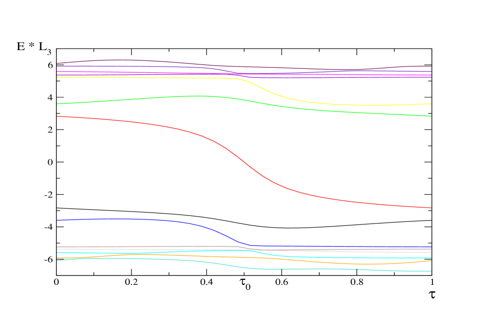
Figure 9: Spectral flow of the left handed eigenmodes of the Dirac Hamiltonian for non orthogonally intersecting vortices depending on $x_{4}/L_{4}$. The vortices cross at $x_{4}=L_{4}/2$, i.e. at $\tau=\tau_{0}=0.5$.

The probability densities of the eigenvectors of the Dirac Hamiltonian again show an enhancement at the position of the vortices, see fig. 10.

Figure 10: Probability density of the eigenmode of the Dirac Hamiltonian whose energy eigenvalue crosses zero where the parameters in eq. (4.3) have been chosen to be $u^{(0)}=0.3+i0.5$, $v^{(0)}=0.3$ at $x_{3}=0.3L_{3},x_{4}=0.29$ and $x_{3}=0.3,x_{4}=0.52$, respectively.

5 Concluding remarks

We have studied the quark spectrum in the background of intersecting flat vortex sheets. Choosing the four-torus ${\mathbb{T}}^{4}$ as space-time manifold we have calculated the spectral flow of the Dirac Hamiltonian as function of time for intersecting vortex fields. The spectral flow as function of time $\tau$ has the largest gradient in the neighborhood of the vortex intersection point, i.e. where the topological charge is localized. For the infinitely thick intersecting “vortices” considered in section 2 this gradient is constant (see eq. (2.28)) reflecting the fact that in this case the topological charge is homogeneously distributed over space-time. These results are consistent with the findings of ref. [16] that zero modes of the 4-dimensional Dirac operator are localized at the intersection points of vortices. Also, the probability density of the quark eigenmodes of the Dirac Hamiltonian considered in the present paper show a strong correlation to the position of the vortex sheets. Depending on the energy level considered, the vortices seem to attract or repel the quarks. For the lowest lying states the probability density always shows an enhancement at the position of the vortices, i.e. the vortices “act attractively” on the quarks in these modes.

6 Acknowledgments

The authors are grateful to O. Schröder for helpful discussions. This work has been supported by the Deutsche Forschungsgemeinschaft under grants DFG-Re 856/5-1.

Appendix A Conventions

We choose the generators of the gauge group to be anti-hermitian. Therefore the components $A_{\mu}$ of the gauge potential are anti-hermitian, e.g. purely imaginary for the gauge group $U(1)$. The magnetic flux $\Phi$ through a closed loop ${\mathcal{C}}$ is defined by

$$\Phi=\frac{1}{2\pi i}\oint_{\mathcal{C}}A_{\mu}{\mathrm{d}}x_{\mu}$$ (A.1)

and thus real valued.

We consider the Dirac equation in Euclidean space-time. In $D=4$ we use the chiral representation for the Dirac matrices:

$$\gamma_{i} = \left(\begin{array}[]{cc}0&\sigma_{i}\\ \sigma_{i}&0\end{array}\right)\,,\quad i=1,2,3\,,\quad\gamma_{4}=\left(\begin{array}[]{cc}0&i{\mathbbm{1}}\\ -i{\mathbbm{1}}&0\end{array}\right)\,,$$ (A.6)

$$\gamma_{5} = \gamma_{1}\gamma_{2}\gamma_{3}\gamma_{4}=\left(\begin{array}[]{cc}{\mathbbm{1}}&0\\ 0&-{\mathbbm{1}}\end{array}\right)\,,$$ (A.9)

where ${\mathbbm{1}}$ is the $2\times 2$ unit matrix and $\sigma_{i}$ are the (hermitian) Pauli matrices.

The massless Dirac Hamiltonian $H$ in three dimensions reads

$$H=-\gamma_{4}\gamma_{i}{\mathrm{D}}_{i}=\left(\begin{array}[]{cc}-i\sigma_{i}{\mathrm{D}}_{i}&0\\ 0&i\sigma_{i}{\mathrm{D}}_{i}\end{array}\right)\,,$$ (A.10)

where ${\mathrm{D}}_{i}=\partial_{i}+A_{i}$ is the covariant derivative.

In this paper we use the theta function conventions introduced in [21]:

$$\theta(z,i{\xi})=\sum_{n\in{\mathbb{Z}}}e^{-\pi{\xi}n^{2}+2\pi inz}\,,\quad z\in{\mathbb{C}}\,,\,{\xi}\in{\mathbb{R}}_{+}\,.$$ (A.11)

These functions are analytic in $z$ and obey the periodicity properties

$$\theta(z+1,i{\xi})=\theta(z,i{\xi})\,,\quad\theta(z+i{\xi},i{\xi})=e^{\pi{\xi}-2\pi iz}\theta(z,i{\xi})\,.$$ (A.12)

The only zeros of this function are at the points [21]

$$z=(m+1/2)+(n+1/2)i{\xi}\,,\quad m,n\in{\mathbb{Z}}\,.$$ (A.13)

Appendix B Zero mode of the Dirac operator in $D=4$

We consider the gauge potential

$$A_{1} = -2\pi ix_{2}/(L_{1}L_{2})\,,\quad A_{2}=0\,,$$ (B.1)

$$A_{3} = -2\pi ix_{4}/(L_{3}L_{4})\,\,,\quad A_{4}=0\,$$ (B.2)

on the four-torus with transition functions

$$U_{1}=U_{3}={\mathbbm{1}}\,,\quad U_{2}=\exp{(-2\pi ix_{1}/L_{1})}\,,\quad U_{4}=\exp{(-2\pi ix_{3}/L_{3})}\,.$$ (B.3)

The topological charge of this configuration is $1$, i.e. there is one (left handed) zero mode of the corresponding Dirac operator which can be written down explicitly in terms of theta functions. To this end one introduces complex variables $u:=(x_{1}+ix_{2})/L_{1}\,,\,v:=(x_{3}+ix_{4})/L_{3}$ and positive real numbers $\tau_{12}:=L_{2}/L_{1}\,,\,\tau_{34}:=L_{4}/L_{3}$. The problem of finding the zero mode becomes a problem of finding the zero mode of the Dirac operator ${{{{\mathrm{D}/\hskip 1.99997pt}_{(2)}}}}=i\sigma_{1}D_{1}+i\sigma_{2}D_{2}$ on the two-torus and this problem can be easily solved (compare [16, 20]). The zero mode of ${{{{\mathrm{D}/\hskip 1.99997pt}_{(2)}}}}$ is given by

$$\phi_{0}=\left(\begin{array}[]{c}0\\ {{\tilde{\varphi}_{0}}}(x_{1},x_{2},L_{1},L_{2})\end{array}\right)\,,\quad{{\tilde{\varphi}_{0}}}(x_{1},x_{2},L_{1},L_{2})=\exp{\left(-\frac{\pi x_{2}^{2}}{L_{1}L_{2}}\right)}\overline{\theta(u,iL_{2}/L_{1})}\,.$$ (B.4)

A short calculation shows that the zero mode in $D=4$ dimensions has the form:

$$\psi_{0}=\left(\begin{array}[]{c}0\\ 0\\ 0\\ {{\tilde{\varphi}_{0}}}(x_{1},x_{2},L_{1},L_{2}){{\tilde{\varphi}_{0}}}(x_{3},x_{4},L_{3},L_{4})\end{array}\right)\,.$$ (B.5)

Obviously, the non-zero spinor component of $\psi_{0}$ is the product of the two zero mode functions ${{\tilde{\varphi}_{0}}}$ from $D=2$.

References

- [1] G. ’t Hooft. On the phase transition towards permanent quark confinement. Nucl. Phys., B138:1, 1978.
- [2] G. Mack and V. B. Petkova. Comparison of lattice gauge theories with gauge groups Z(2) and SU(2). Ann. Phys., 123:442, 1979.
- [3] J. Greensite. The confinement problem in lattice gauge theory. hep-lat/0301023.
- [4] M. Engelhardt, K. Langfeld, H. Reinhardt, and O. Tennert. Deconfinement in SU(2) Yang-Mills theory as a center vortex percolation transition. Phys. Rev., D61:054504, 2000.
- [5] T. G. Kovacs and E. T. Tomboulis. Computation of the vortex free energy in SU(2) gauge theory. Phys. Rev. Lett., 85:704–707, 2000.
- [6] L. del Debbio, M. Faber, J. Greensite, and S. Olejnik. Center dominance and Z(2) vortices in SU(2) lattice gauge theory. Phys. Rev., D55:2298–2306, 1997.
- [7] P. de Forcrand and M. D’Elia. On the relevance of center vortices to QCD. Phys. Rev. Lett., 82:4582–4585, 1999.
- [8] F. Karsch. Deconfinement and chiral symmetry restoration. hep-lat/9903031
- [9] C. Gattringer, P. E. L. Rakow, A. Schäfer, and W. Soldner. Chiral symmetry restoration and the Z(3) sectors of QCD. Phys. Rev., D66:054502, 2002.
- [10] M. Engelhardt and H. Reinhardt. Center vortex model for the infrared sector of Yang-Mills theory: Confinement and deconfinement. Nucl. Phys., B585:591–613, 2000.
- [11] M. Engelhardt, M. Faber, and H. Reinhardt. Center vortex model for the infrared sector of Yang-Mills theory. Nucl. Phys. Proc. Suppl., 106:655–657, 2002.
- [12] H. Reinhardt. Topology of center vortices. Nucl. Phys., B628:133–166, 2002.
- [13] M. Engelhardt and H. Reinhardt. Center projection vortices in continuum Yang-Mills theory. Nucl. Phys., B567:249, 2000.
- [14] J. M. Cornwall. Center vortices, nexuses, and fractional topological charge. Phys. Rev., D61:085012, 2000.
- [15] M. F. Atiyah, V. K. Patodi, and I. M. Singer. Spectral asymmetry and Riemannian geometry 3. Math. Proc. Cambridge Phil. Soc., 79:71, 1980.
- [16] H. Reinhardt, O. Schröder, T. Tok, and V. C. Zhukovsky. Quark zero modes in intersecting center vortex gauge fields. Phys. Rev., D66:085004, 2002.
- [17] N. H. Christ. Conservation law violation at high-energy by anomalies. Phys. Rev., D21:1591, 1980.
- [18] V. V. Khoze. Fermion number violation in the background of a gauge field in Minkowski space. Nucl. Phys., B445:270–294, 1995.
- [19] F. R. Klinkhamer and Y. J. Lee. Spectral flow of chiral fermions in nondissipative gauge field backgrounds. Phys. Rev., D64:065024, 2001.
- [20] S. Azakov. The Schwinger model on the torus. Fortsch. Phys., 45:589–626, 1997.
- [21] D. Mumford. Tata-Lectures about Theta I. Birkhäuser, Boston, 1993.