The Yang Mills^∗ Gravity Dual

David E. Crooks and Nick Evans Department of Physics, Southampton University, Southampton, S017 1BJ, UK

ABSTRACT

We describe a ten dimensional supergravity geometry which is dual to a gauge theory that is non-supersymmetric Yang Mills in the infra-red but reverts to $N$=4 super Yang Mills in the ultra-violet. A brane probe of the geometry shows that the scalar potential of the gauge theory is stable. We discuss the infra-red behaviour of the solution. The geometry describes a Schroedinger equation potential that determines the glueball spectrum of the theory; there is a mass gap and a discrete spectrum. The glueball mass predictions match previous AdS/CFT Correspondence computations in the non-supersymmetric Yang Mills theory, and lattice data, at the 10$\%$ level. Based on a talk presented at SCGT02 in Nagoya, Japan.

1 Introduction

Dualities between gauge theories and string theories follow naturally from the discovery of branes. The Born Infeld action for the brane (like the Nambu-Goto string action) has a dual interpretation as either describing a brane embedded in a space-time or as a field theory living on the brane’s surface. The position of the brane in the bulk can equally be thought of as a scalar vacuum expectation value in the field theory. The first example of such a duality was the $AdS$/CFT Correspondence [1] which is a duality between the conformal $N$=4 super Yang Mills theory and IIB strings (supergravity) on five dimensional Anti-de-Sitter space cross a five sphere. The field theory’s global symmetries (an SO(2,4) superconformal symmetry and an SU(4)_R symmetry) match to space-time symmetries of the $AdS$ space and the five sphere respectively. The supergravity fields enter the field theory in symmetry invariant ways and so appear as sources (eg masses) for field theory operators. The radial direction in $AdS$ has the conformal symmetry properties of an energy scale and has been interpreted as renormalization group scale. Thus the radial behaviour of the supergravity fields describes the RG flow of the field theory sources. Expectation values of operators in the field theory are obtained from derivatives with respect to these sources on the supergravity partition function. The need to take derivatives suggests the duality should hold in the presence of non-zero values for these sources. We should therefore be able to study all possible deformations of the $N$=4 super Yang Mills theory.

Techniques for introducing these deformations [2, 3, 4, 5] and learning how to interpret them [6, 7, 8] have been developed over recent years. The cleanest example [5] involves the introduction of a vev for the six adjoint scalar fields ($tr\phi_{i}\phi_{j}$) by allowing a supergravity scalar field in the 20 representation of SU(4)_R to be non-zero. Solutions of the five dimensional truncated supergravity theory can be found but to interpret these geometries they have been lifted to ten dimensions. In ten dimensions the solutions can, for example, be brane probed [8] and placed in appropriate coordinates where they become multi-centre D3 brane solutions. The original geometry was found from that around a stack of D3 branes whose surface theory is the $N$=4 gauge theory. Moving the branes apart, as in the multi-centre solutions, places the theory on its moduli space and provides a natural gravity dual in the presence of scalar vevs. The deformation program reproduced these geometries and therefore seems to work well!

Here we will describe an on going attempt [9] to describe a non-supersymmetric gauge theory using this technology. The four adjoint fermions of the supersymmetric theory will be made massive via a non-zero five dimensional supergravity field. The solution will be lifted to a complete ten dimensional solution. Brane probing then reveals the scalar potential and we will see that the fermion mass radiatively generates a bounded mass for the six scalar fields. The deep infra-red of this theory is therefore just a gauge field. The ultra-violet theory is still the strongly coupled and conformal $N$=4 theory. Since the UV is strongly coupled there will never be a complete decoupling of the massive matter fields from the dynamics. The goal is to find a theory with the generic properties of QCD and only time will tell how good it is as a numerical approximation. As a first step towards uncovering the physics encoded by the geometry we study the $O^{++}$ glueballs of the theory [10]. The appropriate Schroedinger equation potential [11, 6] is a bounded well (providing further evidence of the stability of the solution) and showing that there is both a mass gap and a discrete glueball spectrum. We determine the spectrum and compare to the results [11] from Witten’s thermal AdS-Schwarzchild geometry [1] and lattice simulations [12] of the non-supersymmetric spectrum. Remarkably the results agree at the 10$\%$ level suggesting this approach may become a useful tool in studying the non-supersymmetric theory.

2 The Deformation in Five Dimensions

We will introduce an equal mass for the four adjoint fermions of the $N$=4 theory via a five dimensional supergravity scalar in the 10 of SU(4)_R. The appropriate scalar, $\lambda$, and its potential can be found in [3] ($V=-{3\over 2}\left[1+\cosh^{2}\lambda\right]$) We look for solutions where $\lambda$ varies in the radial direction, $r$, of $AdS$ and the metric is described by

$$ds_{(1,4)}^{2}=e^{2A(r)}dx^{\mu}dx_{\mu}+dr^{2}$$ (1)

where $\mu=0..3$.

The equation of motion for the scalar fields are [2]

$$\lambda^{{}^{\prime\prime}}+4A^{{}^{\prime}}\lambda^{{}^{\prime}}={\partial V\over\partial\lambda},\hskip 28.45274pt-3A^{{}^{\prime\prime}}-6A^{{}^{\prime}2}=\lambda^{{}^{\prime}2}+2V$$ (2)

Asymptotically, where the geometry returns to $AdS$, the solutions are

$$\lambda=Me^{-r}+Ke^{-3r}$$ (3)

Corresponding to a mass and a vev for our fermionic operator.

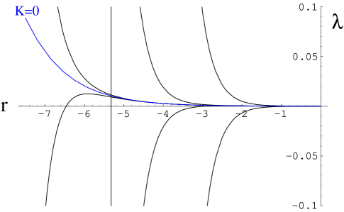
Figure 1: Numerical solutions of the 5d supergravity equations for the scalar $\lambda$. The $K$=0 flow corresponds to the mass only boundary conditions.

Numerical solution of these equations are displayed in figure 1 for different asymptotic boundary conditions. The mass only flow is a unique flow - in the presence of any condensate the flows clearly diverge. Finding the final fate of the mass only flow numerically requires arbitrary fine tuning of the initial conditions. However, from figure 1 it seems likely the flow diverges in the very deep infra-red. The interpretation of such singularities remains open. For example the backgrounds describing $N$=4 SYM on moduli space are singular but those singularities are understood to correspond to the presence of D3 branes in the solution. In the $N$=2^∗ theory [7] the singularities correspond to the divergence of the running gauge coupling. This latter case is the most likely explanation of the divergence here. We will see that a well defined glueball spectrum emerges from this geometry in spite of the divergence suggesting it is not a disaster!

Interpreting the five dimensional geometries has proven hard so we will move to the lift of the solution to ten dimensions.

3 The Ten Dimensional Lift

Lifting the five dimensional solutions to ten seems like a tough task but Pilch and Warner have made an ansatz [3] for the form of the metric and dilaton. The remaining ten dimensional forms can then be found from the equations of motion (after much work!). The lift is described in detail in [9] but here we will just present the results.

Asymptotically the scalar in the 10 lifts to a 3-form potential

$$A_{(2)}=2\lambda(i\cos^{3}\alpha\cos\theta_{+}d\theta_{+}\wedge d\phi_{+}-\sin^{3}\alpha\cos\theta_{-}d\theta_{-}\wedge d\phi_{-})$$ (4)

We have written the five-sphere as two 2-spheres ($d\Omega_{\pm}^{2}=d\theta_{\pm}^{2}+\sin^{2}\theta_{\pm}d\phi_{\pm}^{2}$) and an angle $\alpha$ between them.

The full solution has all the ten dimensional fields switch on. The metric is given by

$$ds_{10}^{2}=(\xi_{+}\xi_{-})^{1\over 2}ds_{1,4}^{2}+(\xi_{+}\xi_{-})^{-{3\over 2}}ds_{5}^{2}$$ (5)

$$ds_{5}^{2}=\xi_{-}\cos^{2}\alpha~{}d\Omega_{+}^{2}+\xi_{+}\sin^{2}\alpha~{}d\Omega_{-}^{2}+\xi_{+}\xi_{-}d\alpha^{2}$$ (6)

where the $\xi_{\pm}$ are given by

$$\xi_{\pm}=c^{2}\pm s^{2}\cos 2\alpha,\hskip 14.22636ptc=\cosh\lambda,\hskip 14.22636pts=\sinh\lambda$$ (7)

The dilaton is given, in unitary gauge, by the functions

$$f={1\over\xi^{1/2}}\sqrt{\cosh^{2}\lambda+(\xi_{+}\xi_{-})^{1/2}\over 2},\hskip 28.45274ptB={\sinh^{2}\lambda\cos 2\alpha\over\cosh^{2}\lambda+(\xi_{+}\xi_{-})^{1/2}}$$ (8)

In the more usual language the axion-dilaton field is given by

$$C+ie^{-\Phi}=i{(1-B)\over(1+B)}$$ (9)

Thus for this solution the $\theta$ angle is switched off.

The two-form potential is given by

$$A_{(2)}=iA_{+}\cos^{3}\alpha\,\cos\theta_{+}d\theta_{+}\wedge d\phi_{+}-A_{-}\sin^{3}\alpha\,\cos\theta_{-}d\theta_{-}\wedge d\phi_{-}$$ (10)

with

$$A_{\pm}=\sinh 2\,\lambda/\xi_{\pm}$$ (11)

Finally the four-form potential lifts to

$$F_{(4)}=F+\star F,\hskip 14.22636ptF=dx^{0}\wedge dx^{1}\wedge dx^{2}\wedge dx^{3}\wedge d\omega$$ (12)

where

$$\omega(r)=e^{4A(r)}A^{\prime}(r)$$ (13)

4 Brane Probing

As a first exploration of this geometry we can place a probe D3 brane in the geometry. At leading order in $1/N$ we can neglect the back reaction of the probe on the geometry. Substituting the geometry into the Born Infeld action for the probe

$$S_{probe}=-\tau_{3}\int_{\mathcal{M}_{4}}d^{4}x\det[G^{(E)}_{ab}+2\pi\alpha^{\prime}e^{-\Phi/2}F_{ab}]^{1/2}+\mu_{3}\int_{\mathcal{M}_{4}}C_{4},$$ (14)

will reveal the field theory on the brane’s surface. We find a potential

$$V_{probe}=e^{4A}\left[\xi_{+}\xi_{-}-A^{{}^{\prime}}\right]$$ (15)

It is illuminating to evaluate this potential at leading order in the ultra-violet with $\lambda=Me^{-r}$, $A=r$, which gives

$$V=M^{2}e^{2r}+...$$ (16)

The field $e^{r}$ has conformal dimension 1 and should be identified with the scalar fields of the field theory. This term corresponds to an equal, bounded mass for the six scalars. This confirms field theory expectations that when supersymmetry is broken via the fermion mass the scalars will radiatively acquire a mass. It is also encouraging that the theory has a bounded potential.

5 The Glueball Spectrum

We can make an initial investigation of the infra-red properties of the gauge theory described by our geometry as follows. The $O^{++}$ glueballs of the theory have been identified [11] with excitations of the dilaton field of the form

$$\delta\Phi=\psi(r)e^{-ikx},\hskip 28.45274ptk^{2}=-M^{2}$$ (17)

This deformation must be a solution of the 5d dilaton field equation $\partial_{\mu}(\sqrt{-g}g^{\mu\nu}\partial_{\nu})\delta\Phi=0$. If we make the change of coordinates [6] ($r\rightarrow z$) such that

$${dz\over dr}=e^{2A},\hskip 28.45274pt\psi\rightarrow e^{-3A/2}\psi$$ (18)

Then the dilaton field equation takes a Schroedinger form

$$(-\partial_{z}^{2}+V(z))\psi(z)=M^{2}\psi(z)$$ (19)

where

$$V={3\over 2}A^{{}^{\prime\prime}}+{9\over 4}(A^{{}^{\prime}})^{2}$$ (20)

Solving the equations of motion in these coordinates and tuning onto the mass only solution produces the well potential shown in figure 2 [10]. Note that if any condensate is present the

Figure 2: The Schroedinger potential for the $O^{++}$ glueballs and the lowest lying solutions.

well becomes unstable at large $z$. In the massive case the potential well shows us that there is a mass gap and a discrete glueball spectrum. The gauge theory dual is confining in the infra-red.

The glueball spectrum can be obtain using the numerical shooting technique and the three lowest energy solutions are shown in figure 2. We therefore have predictions for the lightest $O^{++}$ glueball states, shown in table 1. The lightest state’s mass is not a prediction but can be used to fix the value of $\Lambda_{QCD}$ - we normalize it to the lattice results discussed below. It is interesting to compare to other computations of these masses. Witten [1] found a high temperature deformation of the gravity dual of the field theory on the surface of an M5 brane which is expected at low energies to describe 4 dimensional non-supersymmetric Yang Mills theory (but in the UV has many extra adjoint matter fields and lives in 6 dimensions). Similar techniques were used to determine the predicted glueball masses [11] and are shown in Table 1. They match remarkably well with our results suggesting that the high energy completion of the theory is relatively unimportant. We also display the limited lattice results in non-supersymmetric Yang Mills in the table and again the agreement is at the 10$\%$ level although we only have the one excited state result for comparison.

	YM∗	AdS-Schwarz	Lattice
O++	1.6 (input)	1.6 (input)	$1.6\pm 0.15$
O++∗	2.4	2.6	$2.48\pm 0.23$
O++∗∗	3.1	3.5	?

Table 1: Glueball mass predictions from the $AdS$/CFT Correspondence and lattice calculations.

Encouragingly the Yang Mills^∗ gravity dual appears to encode much of the physics we would expect of non-supersymmetric Yang Mills theory. The obvious next challenge is to include quark fields which we are currently working on.

6 Acknowledgements

DEC is grateful to PPARC for the support of a studentship. NE is grateful to PPARC for the support of an Advanced Fellowship.

References

- [1] J. Maldacena, Adv. Theor. Math. Phys. 2 231 (1998), hep-th/9711200; S.S. Gubser, I.R. Klebanov and A.M. Polyakov, Phys. Lett. B428 105 (1998), hep-th/9802109; E. Witten, Adv. Theor. Math. Phys. 2 253 (1998), hep-th/9802150.
- [2] L. Girardello, M. Petrini, M. Porrati and A. Zaffaroni, JHEP 9812 022 (1998), hep-th/9810126; L. Girardello, M. Petrini, M. Porrati and A. Zaffaroni,JHEP 9905 026 (1999), hep-th/9903026.
- [3] A. Khavaev, K. Pilch and N. P. Warner, Phys. Lett. B487 14 (2000), hep-th/9812035.
- [4] L. Girardello, M. Petrini, M. Porrati and A. Zaffaroni, Nucl.Phys. B569 451 (2000), hep-th/9909047.
- [5] D. Z. Freedman, S. S. Gubser, K. Pilch and N. P. Warner, JHEP 0007 038 (2000), hep-th/9906194.
- [6] S.S. Gubser, Adv. Theor. Math. Phys. 4 679 (2002), hep-th/0002160.
- [7] K. Pilch, N.P. Warner, Adv. Theor. Math. Phys. 4 627 (2002), hep-th/0006066; A. Brandhuber, K. Sfetsos, Phys. Lett. B488 373 (2000), hep-th/0004148; A. Buchel, A.W. Peet and J. Polchinksi, Phys. Rev. D63 044009 (2001), hep-th/0008076; N. Evans, C.V. Johnson and M. Petrini, JHEP 0010 022 (2000), hep-th/0008081.
- [8] J. Babington, N. Evans, J, Hockings, JHEP 0107 034 (2001), hep-th/0105235.
- [9] J. Babington, D.E. Crooks, N. Evans, to appear in Phys. Rev D, hep-th/0210068.
- [10] D.E. Crooks, N. Evans, preprint in preparation.
- [11] C. Csaki, H. Ooguri, Y. Oz, J. Terning, JHEP 9901 017 (1999), hep-th/9806021.
- [12] M. Teper, hep-lat/0203203; C.J. Morningstar, M.J. Peardon, Phys. Rev. D60 034509 (1999), hep-lat/9901004.