OU-HET 430

hep-th/0302090
Feb 2003

A New Class of Conformal Field Theories with Anomalous Dimensions

Kiyoshi Higashijima and Etsuko Itou

Department of Physics, Graduate School of Science, Osaka University,
Toyonaka, Osaka 560-0043, Japan

The Wilsonian renormalization group (WRG) equation is used to derive a new class of scale invariant field theories with nonvanishing anomalous dimensions in $2$-dimensional ${\cal N}=2$ supersymmetric nonlinear sigma models. When the coordinates of the target manifolds have nontrivial anomalous dimensions, vanishing of the $\beta$ function suggest the existence of novel conformal field theories whose target space is not Ricci flat. We construct such conformal field theories with ${\bf U}(N)$ symmetry. The theory has one free parameter $a$ corresponding to the anomalous dimension of the scalar fields. The new conformal field theories are well behaved for positive $a$, while they have curvature singularities at the boundary for $a<0$. When the target space is of complex $1$-dimension, we obtain the explicit form of the Lagrangian, which reduces to two different kinds of free field theories in weak and in strong coupling limit. The target space in this case looks like a semi-infinite cigar with one-dimension compactified to a circle.

1 Introduction

Nonlinear sigma models (NL$\sigma$Ms) in two dimensions are interesting for several reasons. They help us to understand various non-perturbative phenomena in four dimensional gauge theories such as confinement or dynamical mass generation [1, 2]. They also provide the description of superstrings propagating in the curved space-time. In the latter case, the consistency of strings requires the ${\cal N}=2$ superconformal symmetry of the NL$\sigma$Ms. Since ${\cal N}=2$ supersymmetry and the scale invariance imply ${\cal N}=2$ superconformal symmetry, these NL$\sigma$Ms have to be scale invariant. In quantum field theories, the scale invariance, suffering from anomaly due to the divergent renormalization effects, is realized only at the fixed-points of the renormalization group equation. Since field theories at the fixed-point also describes the phase transition, it is important to study these fixed-point theories of ${\cal N}=2$ supersymmetric NL$\sigma$Ms.

In ${\cal N}=2$ supersymmetric NL$\sigma$Ms, the field variables take values on the complex curved spaces called Kähler manifolds, whose metrics are specified completely by the Kähler potentials. These Kähler potentials, arbitrary functions of the chiral superfields, have infinite numbers of coupling constants since any NL$\sigma$M is renormalizable in perturbation theories in two dimensions. It is convenient to use the Wilsonian renormalization group (WRG) equation for the nonperturbative study of field theories with infinite numbers of coupling constants. In a previous paper, we derived the $\beta$ function for $2$-dimensional ${\cal N}=2$ supersymmetric NL$\sigma$M using the WRG equation[3, 4, 5]:

$$\beta(g_{i\bar{j}})=\frac{1}{2\pi}R_{i\bar{j}}+\gamma\Big{[}\varphi^{k}g_{i\bar{j},k}+\varphi^{*\bar{k}}g_{i\bar{j},\bar{k}}+2g_{i\bar{j}}\Big{]}.$$ (1.1)

The WRG equation shows the variation of Wilsonian effective action when the cutoff scale is changed [6, 7, 8, 9]. The first term, proportional to the Ricci tensor of the target space, comes from the one-loop diagrams, whereas the second term, proportional to the anomalous dimension $\gamma$ of fields, comes from the rescaling of fields to normalize the kinetic term properly. The presence of the anomalous dimension reflects the nontrivial continuum limit of the fields.

When the anomalous dimension of the field vanishes, the scale invariance is realized for NL$\sigma$Ms on the Ricci-flat Kähler (Calabi-Yau) manifolds [10]. Calabi-Yau metrics for some noncompact manifolds have been explicitly constructed [11], when the number of isometries is sufficient to reduce the Einstein equation to an ordinary differential equation.

On the other hand, when the anomalous dimension of fields does not vanish, the condition of the scale invariance is quite different. In this article, we study the novel conformal field theories with anomalous dimension by solving the condition of the fixed-point: $\beta=0$. We will assume ${\bf U}(N)$ symmetry to reduce a set of the partial differential equations to an ordinary differential equation. The conformal theories obtained have one free parameter corresponding to the anomalous dimension of the scalar fields. The geometry of the target manifolds crucially depends on the sign of the anomalous dimensions.

This paper is organized as follow: In §2, we review briefly the WRG equation for $2$ dimensional ${\cal N}=2$ supersymmetric nonlinear sigma model. In §3, we derive the condition of scale invariance assuming the ${\bf U}(N)$ symmetry. In §4, we study the geometry of target spaces of conformal field theories. In §5, the properties of the new conformal field theories are discussed.

2 Wilsonian Renormalization Group equation

In this section, let us recapitulate the Wilsonian renormalization group equation for the ${\cal N}=2$ supersymmetric NL$\sigma$M. The Wilsonian renormalization group equation describes the variation of effective action when the cutoff energy scale $\Lambda$ is changed to $\Lambda(\delta t)=\Lambda e^{-\delta t}$ in $D$ dimensional field theory [6, 7, 8, 9]:

$$\frac{d}{dt}S[\Omega;t] = \frac{1}{2\delta t}\int_{p^{\prime}}\mathop{\mathrm{tr}}\nolimits\ln\left(\frac{\delta^{2}S}{\delta\Omega^{i}\delta\Omega^{j}}\right)$$

$$-\frac{1}{2\delta t}\int_{p^{\prime}}\int_{q^{\prime}}\frac{\delta S}{\delta\Omega^{i}(p^{\prime})}\left(\frac{\delta^{2}S}{\delta\Omega^{i}(p^{\prime})\delta\Omega^{j}(q^{\prime})}\right)^{-1}\frac{\delta S}{\delta\Omega^{j}(q^{\prime})}$$

$$+\left[D-\sum_{\Omega_{i}}\int_{p}\hat{\Omega}_{i}(p)\left(d_{\Omega_{i}}+\gamma_{\Omega_{i}}+\hat{p}^{\mu}\frac{\partial}{\partial\hat{p}^{\mu}}\right)\frac{\delta}{\delta\hat{\Omega}_{i}(p)}\right]\hat{S},$$

where $d_{\Omega}$ and $\gamma_{\Omega}$ denote the canonical and anomalous dimensions of the field $\Omega$. The caret indicates dimensionless quantities. The first and second terms in eq.(LABEL:WRG-1) correspond to the one-loop and tree diagrams where internal lines are eliminated fields with high momentum $\Lambda(\delta t)<p<\Lambda$. The remaining terms come from the rescaling of fields to normalize the coefficient of the kinetic term to unity.

This WRG equation is an infinite set of differential equations for various coupling constants in the most general action $S$. In practice, we usually expand the action in power of derivatives and retain the first few terms. We often introduce symmetry to further reduce the number of independent coupling constants.

We impose ${\cal N}=2$ supersymmetry on the action and consider only Kähler potential term to define the ${\cal N}=2$ supersymmetric nonlinear sigma model in two dimensions

$$S = \int d^{2}\theta d^{2}\bar{\theta}d^{2}xK[\Phi,\Phi^{\dagger}]$$ (2.2)

$$= \int d^{2}x\Bigg{[}g_{n\bar{m}}\left(\partial^{\mu}\varphi^{n}\partial_{\mu}\varphi^{*\bar{m}}+\frac{i}{2}\bar{\psi}^{\bar{m}}\sigma^{\mu}(D_{\mu}\psi)^{n}+\frac{i}{2}\psi^{n}\bar{\sigma}^{\mu}(D_{\mu}\bar{\psi})^{\bar{m}}+\bar{F}^{\bar{m}}F^{n}\right)$$

$$-\frac{1}{2}K_{,nm\bar{l}}\bar{F}^{\bar{l}}\psi^{n}\psi^{m}-\frac{1}{2}K_{,n\bar{m}\bar{l}}F^{n}\bar{\psi}^{\bar{m}}\bar{\psi}^{\bar{l}}+\frac{1}{4}K_{,nm\bar{k}\bar{l}}(\bar{\psi}^{\bar{k}}\bar{\psi}^{\bar{l}})(\psi^{n}\psi^{m})\Bigg{]},$$

where $\Phi^{n}$ denote chiral superfields, whose components fields are complex scalars $\varphi^{n}(x)$, Dirac fermions $\psi^{n}(x)$ and complex auxiliary fields $F^{n}(x)$. The Kähler metric of the target space $g_{i\bar{j}}$ is given by the Kähler potential

$$g_{i\bar{j}}(\varphi,\varphi^{\dagger})=\frac{\partial^{2}K(\varphi,\varphi^{\dagger})}{\partial\varphi^{i}\partial\varphi^{*\bar{j}}}.$$ (2.3)

Higher derivative terms are not included in this paper to avoid the introduction of negative metric states.

For this nonlinear sigma model, the WRG eq.(LABEL:WRG-1) has been derived in Ref.[3]. The scalar part of the WRG equations takes a simple form

$$\frac{d}{dt}\int d^{2}xg_{i\bar{j}}(\partial_{\mu}\varphi)^{i}(\partial^{\mu}\varphi^{*})^{\bar{j}}$$

$$=\int d^{2}x\Big{[}-\frac{1}{2\pi}R_{i\bar{j}}-\gamma\Big{(}\varphi^{k}g_{i\bar{j},k}+\varphi^{*\bar{k}}g_{i\bar{j},\bar{k}}+2g_{i\bar{j}}\Big{)}\Big{]}(\partial_{\mu}\varphi)^{i}(\partial^{\mu}\varphi^{*})^{\bar{j}}.$$

The field variables $\varphi^{n}(x)$ are assumed $t$ independent by a suitable rescaling of fields, which introduces the anomalous dimension $\gamma$ in return. What depends on $t$ is the infinite number of coupling constants included in the Kähler metric. From this WRG equation, the $\beta$ function for the Kähler metric is given by

$$\frac{d}{dt}g_{i\bar{j}} = -\frac{1}{2\pi}R_{i\bar{j}}-\gamma\Big{[}\varphi^{k}g_{i\bar{j},k}+\varphi^{*\bar{k}}g_{i\bar{j},\bar{k}}+2g_{i\bar{j}}\Big{]}$$ (2.5)

$$\equiv -\beta(g_{i\bar{j}}).$$

Note that our $\beta$ function reduces to the Ricci tensor when the anomalous dimension of the fields vanishes. The second term which is proportional to the anomalous dimension $\gamma$ is not reparametrization invariant because of the renormalization condition of the fields breaks reparametrization invariance. The fermion part also gives the same WRG equation because of the supersymmetry. Since the Kähler metric contain the infinite number of coupling constants, the above WRG equation is an infinite set of differential equations for these coupling constants. In the next section, we investigate the conformal theories defined as the fixed-points of this renormalization group equation.

3 Fixed-point of SU(N) symmetric WRG equation

In this section, let us derive the action of the conformal field theory corresponding to the fixed-point of the $\beta$ function

$$\beta(g_{i\bar{j}})=\frac{1}{2\pi}R_{i\bar{j}}+\gamma\Big{[}\varphi^{k}g_{i\bar{j},k}+\varphi^{*\bar{k}}g_{i\bar{j},\bar{k}}+2g_{i\bar{j}}\Big{]}=0.$$ (3.1)

Since Ricci curvature $R_{i\bar{j}}$ is a second derivative of the metric $g_{i\bar{j}}$, the equation is a set of coupled partial differential equations, and is very difficult to solve in general. So we simplify the problem by assuming symmetry ${\bf U}(N)$ for the Kähler potential.

$$K[\varphi,\varphi^{\dagger}] = \sum^{\infty}_{n=1}g_{n}x^{n}\equiv f(x)$$ (3.2)

where $x$ is the ${\bf U}(N)$ invariant combination

$$x\equiv\vec{\varphi}\cdot\vec{\varphi}^{\dagger}$$ (3.3)

of the $N$ components scalar fields $\vec{\varphi}=(\varphi^{1},\varphi^{2},\cdots,\varphi^{N})$. The coefficients $g_{n}$ play the role of an infinite number of coupling constants which depend on the cutoff scale $t$. The Kähler potential gives the Kähler metric and Ricci tensor as follows:

$$g_{i\bar{j}} \equiv \partial_{i}\partial_{\bar{j}}K[\varphi,\varphi^{\dagger}]=f^{\prime}\delta_{i\bar{j}}+f^{\prime\prime}\varphi_{i}^{*}\varphi_{\bar{j}},$$ (3.4)

$$R_{i\bar{j}} \equiv -\partial_{i}\partial_{\bar{j}}\mathop{\mathrm{tr}}\nolimits\ln g_{i\bar{j}}$$

$$= -\Big{[}(N-1)\frac{f^{\prime\prime}}{f^{\prime}}+\frac{2f^{\prime\prime}+f^{\prime\prime\prime}x}{f^{\prime}+f^{\prime\prime}x}\Big{]}\delta_{i\bar{j}}$$

$$-\Big{[}(N-1)\bigg{(}\frac{f^{(3)}}{f^{\prime\prime}}-\frac{(f^{\prime\prime})^{2}}{(f^{\prime})^{2}}\bigg{)}+\frac{3f^{(3)}+f^{(4)}x}{f^{\prime}+f^{\prime\prime}x}-\frac{(2f^{\prime\prime}+f^{\prime\prime\prime}x)^{2}}{(f^{\prime}+f^{\prime\prime}x)^{2}}\Big{]}\varphi^{*}_{i}\varphi_{\bar{j}},$$

where

$$f^{\prime}=\frac{df}{dx}.$$ (3.6)

We substitute these metric and Ricci tensor for the $\beta$ function (2.5) and compare the coefficients of $\delta_{i\bar{j}}$ and $\varphi^{i}\varphi^{*\bar{j}}$ to find

$$\frac{\partial}{\partial t}f^{\prime} = \frac{1}{2\pi}\Big{[}(N-1)\frac{f^{\prime\prime}}{f^{\prime}}+\frac{2f^{\prime\prime}+f^{\prime\prime\prime}x}{f^{\prime}+f^{\prime\prime}x}\Big{]}-2\gamma(f^{\prime}+f^{\prime\prime}x),$$ (3.7)

$$\frac{\partial}{\partial t}f^{\prime\prime} = \frac{1}{2\pi}\Big{[}(N-1)\bigg{(}\frac{f^{(3)}}{f^{\prime\prime}}-\frac{(f^{\prime\prime})^{2}}{(f^{\prime})^{2}}\bigg{)}+\frac{3f^{(3)}+f^{(4)}x}{f^{\prime}+f^{\prime\prime}x}-\frac{(2f^{\prime\prime}+f^{\prime\prime\prime}x)^{2}}{(f^{\prime}+f^{\prime\prime}x)^{2}}\Big{]}$$ (3.8)

$$-2\gamma(2f^{\prime\prime}+f^{\prime\prime\prime}x).$$

Since the second equation (3.8) follows from the first equation by differentiation with respect to $x$, we discuss only the first equation.

Our differential equation (3.7) describes the renormalization group flow in the theory space specified by the infinite number of coupling constant in the Kähler potential. In fact, we can derive an infinite number of coupled differential equations among the coupling constants $g_{n}$ by inserting (3.2) in eq.(3.7). We are specially interested in the fixed-point of eq.(3.7), which is supposed to give a scale invariant theory. The fixed-point theory is defined by the Kähler metric which satisfies the following differential equation

$$\frac{\partial}{\partial t}f^{\prime} = \frac{1}{2\pi}\Big{[}(N-1)\frac{f^{\prime\prime}}{f^{\prime}}+\frac{2f^{\prime\prime}+f^{\prime\prime\prime}x}{f^{\prime}+f^{\prime\prime}x}\Big{]}-2\gamma(f^{\prime}+f^{\prime\prime}x)$$ (3.9)

$$= 0.$$

To obtain the Lagrangian of the scale invariant field theory, we have to solve this differential equation.

By noting that this equation can be rewritten as

$$\frac{d}{dx}\Big{[}\ln(f^{\prime})^{N-1}(f^{\prime}+f^{\prime\prime}x)\Big{]}=4\pi\gamma\frac{d}{dx}(f^{\prime}x),$$ (3.10)

we can integrate it easily to obtain

$$(f^{\prime})^{N-1}F^{\prime}=C_{1}\exp[4\pi\gamma F],$$ (3.11)

where

$$F\equiv f^{\prime}x,$$ (3.12)

and $C_{1}$ is an integration constant. The normalization condition of the kinetic term,

$$g_{i\bar{j}}|_{x=0}=\delta_{i\bar{j}},$$

gives an initial condition

$$f^{\prime}(0)=1,\qquad\mbox{namely}\quad F^{\prime}(0)=1$$ (3.13)

which fixes $C_{1}=1$.

Integrating eq.(3.11), we see that the solution of the differential equation satisfy the following algebraic equation:

$$\frac{e^{aF}}{a}\sum^{N-1}_{r=0}(-1)^{r}\frac{(N-1)!F^{(N-1)-r}}{(N-1-r)!a^{r}}=\frac{1}{N}x^{N}+C_{2}.$$ (3.14)

where we have introduced a constant $a\equiv-4\pi\gamma$, namely, we write the anomalous dimension of the scalar field using a free parameter $a$ as follows:

$$\gamma=-\frac{a}{4\pi}.$$ (3.15)

In NL$\sigma$M, the anomalous dimension of the scalar field can take either positive or negative value, so the parameter $a$ can also take either sign [12]. Setting $x=0$ in eq.(3.14) and using the boundary condition (3.13), we obtain

$$C_{2}=(-1)^{N-1}\frac{(N-1)!}{a^{N}}.$$ (3.16)

From this condition (3.14), we can obtain the function $f^{\prime}=F/x$. Since the metric (3.4) is determined by $f^{\prime}$ and $f^{\prime\prime}$, our Lagrangian is completely fixed by eq.(3.14). Thus we found that the Lagrangian of the scale invariant theory has a free parameter $a$ corresponding to the anomalous dimension of the field.

4 Geometry of the target space of the scale invariant theory

In this section, we study the geometry of target space when the theory is scale invariant.

4.1 One-dimensional target space

This equation (3.14) is very simple when the target manifold is of complex one-dimension. When $N=1$, this equation reads

$$\frac{e^{aF}}{a} = x+\frac{1}{a}$$ (4.1)

which gives

$$f^{\prime}=\frac{1}{ax}\ln(1+ax).$$ (4.2)

Using this $f^{\prime}$ in eq.(3.4) gives the metric of the target space

$$g_{i\bar{j}}=f^{\prime}+f^{\prime\prime}x=\frac{1}{1+ax}.$$ (4.3)

Note that the metric has only one component, and the indices $i$ and $\bar{j}$ is $1$. The scalar curvature is given

$$R=\frac{a}{1+ax}.$$ (4.4)

The property of this target manifold crucially depends on the sign of the parameter $a$.

Now, we investigate the property of the target manifold for each sign of $a$.

1. When $a>0$, the anomalous dimension is negative.
   Since the line element is given by

   $$ds^{2}=\frac{|dz|^{2}}{1+a|z|^{2}},$$ (4.5)

   or in polar coordinate $z=re^{i\phi}$

   $$ds^{2}=\frac{1}{1+ar^{2}}\Big{(}(dr)^{2}+r^{2}(d\phi)^{2}\Big{)},$$ (4.6)

   the volume and the distance from the origin ($r=0$) to infinity ($r=\infty$) is divergent, while the length of the circumference at the infinity is finite. Therefore, the shape of the target manifold is a semi-infinite cigar. The volume integral of the scalar curvature is also finite, giving the Euler number:

   $$\chi=\frac{1}{2\pi}\int dzd\bar{z}(\det g_{i\bar{j}})R=\frac{1}{2\pi}\int dzd\bar{z}\frac{1}{(1+a|z|^{2})^{2}}=1,$$ (4.7)

   which is equal to that of a disc.

   

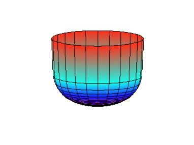
   Figure 1: The target manifold for $a=+1$ embedded in $3$-dimensional flat Euclidean spaces. It looks like a semi-infinite cigar with a radius $\sqrt{\frac{1}{a}}$. Our metric (4.12) is the induced metric on this surface.

   Let us embed the manifold in $3$ dimensional Euclidean spaces. When the hyperplane has the rotational symmetry, the line element can be written using the cylindrical coordinates

   $$ds^{2}=(dh)^{2}+(d\rho)^{2}+\rho^{2}(d\phi)^{2}.$$ (4.8)

   Where the height is a function of the radius $\rho$,

   $$h=g(\rho).$$ (4.9)

   From eq.(4.9), the line element can be rewritten

   $$ds^{2}=(1+(g^{\prime}(\rho))^{2})(d\rho)^{2}+\rho^{2}(d\phi)^{2},$$ (4.10)

   where $g^{\prime}$ is the derivative of the function $g(\rho)$ in term of $\rho$. Now we transform the line element for the target metric (4.3) to the form of eq.(4.10) by a change of variable

   $$\rho=\frac{r}{\sqrt{1+ar^{2}}},$$ (4.11)

   which is a one-to-one mapping from the entire plane $0\leq r<\infty$ to a disc $0\leq\rho<\frac{1}{\sqrt{a}}$. Then eq.(4.6) can be rewritten

   $$ds^{2}=\frac{1}{(1-a\rho^{2})^{2}}(d\rho)^{2}+\rho^{2}(d\phi)^{2}.$$ (4.12)

   Comparing eq.(4.10) with eq.(4.12), we obtain the height function $h=g(\rho)$ as follow:

   $$h = \int_{0}^{\rho}d\rho g^{\prime}(\rho)=\int_{0}^{\rho}d\rho\sqrt{\frac{1}{(1-a\rho^{2})^{2}}-1}$$

   $$= -\frac{1}{2\sqrt{a}}\Big{(}\ln|\frac{\sqrt{2-a\rho^{2}}-1}{\sqrt{2-a\rho^{2}}+1}|+2\sqrt{2-a\rho^{2}}-\ln|\frac{\sqrt{2}-1}{\sqrt{2}+1}|-2\sqrt{2}\Big{)}$$

   . (4.13)

   Figure 1 shows the manifold embedded in $3$-dimensional flat Euclidean spaces. The distance between any two points is measured along the shortest path on the surface in the Euclidean spaces.

2. When $a<0$, the anomalous dimension is positive.
   In this case, the metric and scalar curvature read

   $$g_{i\bar{j}} = \frac{1}{1-|a|x}$$ (4.14)

   $$R = \frac{-|a|}{1-|a|x}.$$ (4.15)

   This metric is ill-defined at the boundary $|z|\sim\frac{1}{\sqrt{-a}}$. It is not merely the coordinates singularity because the scalar curvature is divergent at the boundary. Although the volume integral is divergent, the distance to the boundary is finite. Now, let us embed this manifold in flat space. Note the eq.(4.13) is imaginary if $a<0$. Thus the manifold is embedded as a space-like surface in the flat Minkowski space. Figure 2 shows the manifold embedded in the $3$-dimensional flat Minkowski space.

   

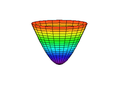
   Figure 2: The target manifold for $a=-1$, embedded in flat Minkowski space. The vertical axis has negative signature. In the asymptotic region $\rho\rightarrow\infty$, the surface approaches to the lightcone.

4.2 Higher dimensional target spaces

Consider the conformal field theories whose target space have more than two dimensions, and investigate the property of the target manifolds. For $N\geq 2$, we have to solve the algebraic equation (3.14) which reads for $N=2$, for example,

$$e^{aF}(aF-1)=\frac{1}{2}(ax)^{2}-1.$$ (4.16)

Figure 3 displays $aF$ as a function of $ax$ for $N=2$ and $|a|=1$.

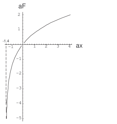
Figure 3: $aF$ as a function of $ax$ for $N=2$ and $|a|=1$. Since $x=zz^{\dagger}$ is positive, $ax\geq 0$ corresponds to $a>0$ while $ax\leq 0$ corresponds to $a<0$.

Kähler potential in the neighborhood of the origin is easily obtained by solving the equation (3.14)

$$f(x)=x-\frac{a}{2(N+1)}x^{2}+\cdots.$$ (4.17)

The asymptotic behaviors crucially depend on the sign of the parameter $a$, so that we will discuss them separately.

1. $a>0$ case
   Figure 3 show the function $f^{\prime}$, which is the diagonal component of the target metric, goes to infinity as $x\rightarrow\infty$. When $aF$ goes to infinity, the $r=0$ term of eq.(3.14) gives the dominant contribution in the left-hand side. To find the asymptotic behavior in this region, we retain only the dominant terms and solve

   $$e^{aF}(aF)^{N-1}\approx\frac{1}{N}(ax)^{N}.$$ (4.18)

   by the iteration method

   $$aF \approx \ln\Big{(}\frac{(ax)^{N}}{N}\Big{)}-(N-1)\ln(aF)$$

   $$= \ln\Big{(}\frac{(ax)^{N}}{N}\Big{)}-(N-1)\ln\ln\Big{(}\frac{(ax)^{N}}{N}\Big{)}+\cdots.$$

   where we dropped other terms that vanish as $ax\rightarrow\infty$. Then we obtain the functions $f^{\prime}$

   $$f^{\prime} \approx \frac{1}{ax}\ln\frac{(ax)^{N}}{N}-\frac{N-1}{ax}\ln\ln\frac{(ax)^{N}}{N}+\cdots.$$ (4.19)

   The distance along the straight line in the radial direction is written

   $$g_{i\bar{j}}dz^{i}dz^{*\bar{j}} = (f^{\prime}\delta_{i\bar{j}}+f^{\prime\prime}z_{\bar{j}}z^{*}_{i})dz^{i}dz^{*\bar{j}}$$ (4.20)

   $$\approx (f^{\prime}+|r|^{2}f^{\prime\prime})|dr|^{2}=\frac{N}{a|r|^{2}}|dr|^{2}$$

   Here we have defined the complex radial coordinate $r$ and the angle variables by

   $$z^{1}=u^{1}r,\ \cdots\ ,\ z^{N-1}=u^{N-1}r,\ z^{N}=r.$$ (4.21)

   The asymptotic behavior (4.20) for any $N$ is similar to $N=1$ case, in which the metric in the asymptotic region is given by

   $$g_{1\bar{1}}\approx\frac{1}{ax}.$$ (4.22)

   The asymptotic behavior of the Kähler potential (3.2) can be found by integrating eq.(4.19)

   $$K(zz^{*}) \approx \frac{N}{2a}(\log{(azz^{*})})^{2}+\cdots$$ (4.23)

   $$= \chi\chi^{*}+2{\sqrt{\frac{N}{a}}}{\mathfrak{R}e}{\chi}\log{\left(1+|u^{1}|^{2}+\cdots+|u^{N-1}|^{2}\right)}+\cdots$$

   where we have dropped holomorphic and anti-holomorphic terms by a Kähler transformation and defined $\chi$ by

   $$\chi=\sqrt{\frac{N}{a}}\log{\sqrt{a}r}.$$ (4.24)

   For fixed values of the radius $r$, (4.23) is the Kähler potential for the Fubini-Study metric of the complex projective space $CP^{N-1}$, whose size is fixed by ${\mathfrak{R}e}{\chi}$. Therefore, our target space is the direct product of the complex line represented by $\chi$ and the $CP^{N-1}$ represented by $(u^{1},\cdots,u^{N-1})$ in the asymptotic region.

2. $a<0$ case
   Figure 3 shows that the allowed region $ax\leq 0$ is limited inside of a ball $|\vec{z}|<(\frac{\sqrt{2}}{|a|})^{\frac{1}{2}}$ for $N=2$ as in the case of $N=1$. By assuming $ax\sim-\sqrt{2}+\epsilon$ near the boundary, we can reduce eq.(4.18) to

   $$e^{aF}aF\sim-\sqrt{2}\epsilon$$

   which can be solved by the iteration method

   $$-aF = \ln\frac{1}{\sqrt{2}\epsilon}+\ln(-aF)$$

   $$= \ln\frac{1}{\sqrt{2}\epsilon}+\ln\ln(\frac{1}{\sqrt{2}\epsilon})+\cdots.$$

   Because of $\epsilon<<1$, the behavior of the function $f^{\prime}=\frac{F}{ax}$ near the boundary is given

   $$f^{\prime}\sim\frac{1}{ax}\ln(1+\frac{ax}{\sqrt{2}}),$$ (4.25)

   which leads to the curvature singularity at the boundary.

   Similarly, the allowed region in $z$-plane for general $N$ is

   $$|\vec{z}|<(N!)^{\frac{1}{2N}}|a|^{-\frac{1}{2}}.$$ (4.26)

   The asymptotic behavior of the function $f^{\prime}$ near the boundary

   $$f^{\prime}(x)\sim\frac{1}{ax}\ln(1+\frac{ax}{(N!)^{1/N}})$$

   leads to the curvature singularity at the boundary.

To summarize, we found that the target spaces of the scale invariant theory with nontrivial anomalous dimension are noncompact and well-behaved at the infinity for $a\geq 0$, while they have formidable curvature singularity at the boundary for $a<0$.

5 Property of the field theory at the fixed-point

In this section, let us discuss the property of the scale invariant field theories for $a\geq 0$. From (4.17), the Kähler potential is given as a power series of $\varphi\varphi^{\dagger}$

$$K(\vec{\varphi}\vec{\varphi}^{\dagger})=\vec{\varphi}\vec{\varphi}^{\dagger}-\frac{a}{2(N+1)}(\vec{\varphi}\vec{\varphi}^{\dagger})^{2}+\cdots.$$ (5.1)

All coefficients in this series are expressed by a single parameter $a$. When $a=0$ this Lagrangian reduces to a free field theory

$${\cal L}=|\partial_{\mu}\vec{\varphi}|^{2}+\frac{i}{2}\bar{\vec{\psi}}\sigma^{\mu}\partial_{\mu}\vec{\psi}+\frac{i}{2}\vec{\psi}\bar{\sigma}^{\mu}\partial_{\mu}\bar{\vec{\psi}}.$$

with the two-point function

$$\langle\varphi^{m}(x)\varphi^{*\bar{n}}(y)\rangle=\delta^{m\bar{n}}\frac{1}{2\pi}\log{\frac{1}{|x-y|}},$$ (5.2)

which corresponds to a vanishing anomalous dimension $\gamma=0$. Higher order terms of $a$ in (5.1) introduce the interaction, which gives the nontrivial anomalous dimension given by (3.15) while $\beta$ function remains zero by the contributions of further higher order terms in (5.1). Although the Lagrangian (5.1) gives a good description for small values of the fields $\varphi(x)$, we have to use another Lagrangian derived from the Kähler potential (4.23) to describe the phenomena for large values of the fields. Equations (4.23) and (4.24) indicate that ${\mathfrak{I}m}{\chi}$ is a periodic variable with a period $2\pi\sqrt{\frac{N}{a}}$. The Kähler potential for the Fubini-Study metric (4.23) implies that the squared radius of the $CP^{N-1}$ is proportional to $2\sqrt{\frac{N}{a}}{\mathfrak{R}e}{\chi}$.

In the presence of the nontrivial anomalous dimension $\gamma$, the two-point function has to behave

$$\langle\varphi^{m}(x)\varphi^{*\bar{n}}(y)\rangle\propto\delta^{m\bar{n}}\frac{1}{|x-y|^{2\gamma}}$$ (5.3)

because of the scale invariance. Although it is difficult to solve field theory with interaction, we can obtain this kind of behavior in the strong coupling limit $a\rightarrow\infty$ of $N=1$ model defined by the metric (4.3). Since the target space approaches to a cylinder at the infinity as is shown in the figure 1, it also approaches to another free field theory when $a$ goes to infinity. In fact, the bosonic part of the Lagrangian for $N=1$ model

$${\cal L}=\frac{1}{1+a|\varphi|^{2}}|\partial_{\mu}\varphi|^{2}$$ (5.4)

reduces to that of a free field theory when $a\rightarrow\infty$

$${\cal L}=|\partial_{\mu}\chi|^{2},$$

where

$$\chi=\frac{1}{\sqrt{a}}\log{(\sqrt{a}\varphi)}.$$ (5.5)

Using this relation (5.5), we can evaluate the two-point function of $\varphi$ by using the free propagator (5.2) for $\chi$

$$\langle\varphi(x)\varphi^{*}(y)\rangle = \frac{1}{a}\langle e^{\sqrt{a}\chi(x)}e^{\sqrt{a}\chi^{*}(y)}\rangle$$ (5.6)

$$= \frac{1}{a}\exp{(a\langle\chi(x)\chi^{*}(y)\rangle)}\propto\frac{1}{|x-y|^{\frac{a}{2\pi}}}.$$

Thus, we find the anomalous dimension of opposite sign in the strong coupling regime. This seems to be an indication that the anomalous dimension aquires higher order corrections in the strong coupling regime. Study of the strong coupling expansion to reconcile this discrepancy is left for future works.

Although the real dimension of the target manifold is two in $N=1$ model, it looks like a cylinder with radius $\sqrt{\frac{1}{a}}$ when viewed from far away places.

6 Conclusion

In order to find non-trivial conformal field theories with anomalous dimension, we used the WRG equation. In solving the WRG equation, we have assumed ${\bf U}(N)$ symmetry to reduce the coupled partial differential equation to an ordinary differential equation. The new class of conformal field theories have one parameter $a$, corresponding to the anomalous dimension of the scalar field. The novel conformal field theories are well behaved for positive $a$, while they have curvature singularities at the boundary for $a<0$. We obtained the Lagrangian explicitly for $N=1$, which allows both the strong and weak coupling expansion. The target space in this case looks like a semi-infinite cigar with one-dimension compactified to a circle. It is interesting to examine the conformal symmetry of our new models both in the weak and in the strong coupling expansion.

After the completion of this work we came to know that our metric was also discussed in other context. The $N=1$ model was proposed by Witten as a model of the two dimensional black hole [13], which was subsequently generalized by Kiritsis, Kounnas and Lust as consistent backgrounds of the superstrings in the presence of the dilaton [14]. Hori and Kapustin proposed to quantize these models by means of linear sigma models with massive gauge field in the Stueckelberg formalism [15].

7 Acknowledgements

This work was supported in part by the Grant-in-Aid for Scientific Research (#13640283 and #13135215). We would like to thank Toshio Nakatsu and Anton Kapustin for pointing out references [13, 14, 15].

References

- [1] A. D’Adda, P. Di Vecchia and M. Luscher, Nucl. Phys. B152 (1979), 125. K.Higashijima, T. Kimura, M. Nitta and M. Tsuzuki, Prog. Theor. Phys. 105 (2001) 261, hep-th/0010272.
- [2] A.Y. Morozov, A.M. Perelomov and M.A. Shifman, Nucl. Phys. B248 (1984) 279.
- [3] K. Higashijima and E. Itou, Prog. Theor. Phys. 108 (2002) 737, hep-th/0205036.
- [4] T.E. Clark, B. Haeri and S.T. Love, Nucl. Phys. B402 (1993) 628, hep-ph/9211261.
- [5] T.E. Clark and S.T. Love, Phys. Rev. D56 (1997) 2461, hep-th/9701134.
- [6] K.G. Wilson and I.G. Kogut, Phys. Rep. 12 (1974) 75.
- [7] F. Wegner and A. Houghton, Phys. Rev. A8 (1973) 401.
- [8] T.R. Morris, Int. J. Mod. Phys. A 9 (1994) 2411, hep-ph/9308265; Phys. Lett. B329 (1994) 241, hep-ph/9403340. T.R. Morris and M.D. Turner, Nucl. Phys. B509 (1998) 637, hep-th/9704202.
- [9] K. Aoki, Int. J. Mod. Phys. B14 (2000) 1249.
- [10] L. Alvarez-Gaumé,D.Z. Freedman and S. Mukhi, Ann.of Phys. (1981) 85.
- [11] K. Higashijima, T. Kimura and M. Nitta, Phys. Lett. B515 (2001) 421, hep-th/0104184; Phys. Lett. B518 (2001) 301, hep-th/0107100; Nucl. Phys. B623 (2002) 133, hep-th/0108084; Ann. Phys. 296 (2002) 347, hep-th/0110216; Nucl. Phys. B645 (2002) 438, hep-th/0202064.
- [12] K. Higashijima and E. Itou, in preparation.
-
[13]
E. Witten, Phys. Rev. D44 (1991) 314.
T. Nakatsu, Prog. Theor. Phys. 87 (1992) 795. - [14] E. Kiritsis, C. Kounnas and D. Lust, Int. J. Mod. Phys. A9 (1994) 1361-1394, hep-th/9308124.
- [15] K. Hori and A. Kapustin, JHEP 0108 (2001) 045, hep-th/0104202; JHEP 0211 (2002) 038, hep-th/0203147.