Black Holes in a Compactified Spacetime

Abstract

We discuss properties of a 4-dimensional Schwarzschild black hole in a spacetime where one of the spatial dimensions is compactified. As a result of the compactification the event horizon of the black hole is distorted. We use Weyl coordinates to obtain the solution describing such a distorted black hole. This solution is a special case of the Israel-Khan metric. We study the properties of the compactified Schwarzschild black hole, and develop an approximation which allows one to find the size, shape, surface gravity and other characteristics of the distorted horizon with a very high accuracy in a simple analytical form. We also discuss possible instabilities of a black hole in the compactified space.

I Introduction

Black hole solutions in a compactified spacetime have been studied in many publications. A lot of attention was paid to Kaluza-Klein higher dimensional black holes. By compactifying black hole solutions along Killing directions one obtains a lower dimensional solutions of Einstein equations with additional scalar, vector and other fields (see e.g. [1] and references therein). The generation of black hole and black string solutions by the Kaluza-Klein procedure was extensively used in the string theory (see e.g. [2] and references therein).

A solution which we consider in this paper is of a different nature. We study a Schwarzschild black hole in a spacetime with one compactified spatial dimension. This dimension does not coincide with any Killing vector, for this reason the black hole metric is distorted as a result of the compactification.

Recent interest in compactified spacetimes with black holes is connected with brane-world models. General properties of black holes in the Randall-Sundrum model were discussed in [4, 5]. In the latter paper 4-dimensional C-metric was used to obtain an exact 3+1 dimensional black hole solution in AdS spacetime with the Randall-Sundrum brane. Black holes in RS braneworlds were discussed in a number of publications (see e.g. [6] and references therein).

Black hole solutions in a spacetime with compactified dimensions are also interesting in connection with other type of brane models, which were considered historically first in [7]. In ADD-type of brane worlds the tension of the brane can be not very large. If one neglects its action on the gravitational field of a black hole, one obtains a black hole in a spacetime where some of the dimensions are compactified. Compactification of special class of solutions, generalized Majumdar-Papapetrou metrics, was discussed by Myers [3]. In this paper he also made some general remarks concerning compactification of the 4-dimensional Schwarzschild metric. Some of the properties of compactified 4-dimensional Schwarzschild metrics were also considered in [8]. For a recent discussion of higher dimensional black holes on cylinders see [9].

In this paper we study a solution describing a 4-dimensional Schwarzschild black hole in a spacetime where one of the dimensions is compactified. This solution is a special case of the Israel-Khan metric [10]. Its general properties were discussed by Korotkin and Nicolai [11]. As a result of the compactification the event horizon of the black hole is distorted. In our paper we focus our attention on the properties of the distorted horizon. We use Weyl coordinates to obtain a solution describing such a distorted black hole. This approach to study of axisymmetric static black holes is well known and was developed long time ago by Geroch and Hartle [12] (see also [18]). In Weyl coordinates, the metric describing a distorted 4-dimensional black hole contains 2 arbitrary functions. One of them, playing a role of the gravitational potential, obeys a homogeneous linear equation. Because of the linearity, one can present the solution as a linear superposition of the unperturbed Schwarzschild gravitational potential, and its perturbation. After this, the second function which enters the solution can be obtained by simple integration. To find the gravitational potential one can either use the Green’s function method or to expand a solution into a series over the eigenmodes. We discuss both of the methods since they give two different convenient representations for the solution. We develop an approximation which allows one to find the size, shape, surface gravity and other characteristics of the distorted horizon with very high accuracy in a simple analytical form. We study properties of compactified Schwarzschild black holes and discuss their possible instability.

The paper is organized as follows. We recall the main properties of 4-D distorted black holes in Section 2. In Section 3, we obtain the solution for a static 4-dimensional black hole in a spacetime with 1 compactified dimension. In Section 4, we study this solution. In particular we discuss its asymptotic form at large distances, and the size, form and shape of the horizon. We conclude the paper by general remarks in Section 5.

II 4-dimensional Weyl black holes

A Weyl form of the Schwarzschild metric

A static axisymmetric 4 dimensional metric in the canonical Weyl coordinates takes the form [12, 15, 18]

$$dS^{2}=-e^{2U}\,dT^{2}+e^{-2U}\,\left[e^{2V}\,(dR^{2}+dZ^{2})+R^{2}\,d\phi^{2}\right]\,,$$ (1)

where $U$ and $V$ are functions of $R$ and $Z$. This metric is a solution of vacuum Einstein equations if and only if these functions obey the equations

$${\partial^{2}U\over\partial R^{2}}+{1\over R}\,{\partial U\over\partial R}+{\partial^{2}U\over\partial Z^{2}}=0\,,$$ (2)

$$V_{,R}=R\,(U_{,R}^{2}-U_{,Z}^{2})\,,\hskip 10.00002ptV_{,Z}=2R\,U_{,R}\,U_{,Z}\,.$$ (3)

Let

$$dl^{2}=dR^{2}+R^{2}\,d\psi^{2}+dZ^{2}\,$$ (4)

be an auxiliary 3 dimensional flat metric, then solutions of (2) coincide with axially symmetric solutions of the 3 dimensional Laplace equation

$$\Delta\,U=0\,,$$ (5)

where $\Delta$ is a flat Laplace operator in the metric (4). It is easy to check that the equation (2) plays the role of the integrability condition for the linear first order equations (3). The regularity condition implies that at regular points of the symmetry axis $R=0$

$$\lim_{R\to 0}\,V(R,Z)=0\,.$$ (6)

In fact, if $V(0,Z_{0})=0$ at any point $Z_{0}$ of $Z$-axis then (3) implies that $V(0,Z)=0$ at any other point of the $Z$-axis which is connected with $Z_{0}$.

For a four dimensional Schwarzschild metric, the function $U$ is the potential of an infinitely thin finite rod of mass $1/2$ per unit length located at $-M\leq Z\leq M$ portion of the $Z$-axis

$$\Delta\,U=4\pi j\,,\hskip 10.00002ptj={1\over 4\pi}{\delta(\rho)\over\rho}\,\Theta(z/M)\,,$$ (7)

where

$$\Theta(x)=\left\{\begin{array}[]{cc}1\,,&\ \ |x|\leq 1\,,\\ 0\,,&\ \ |x|>1\,.\end{array}\right.$$ (8)

The corresponding solution is

$$U_{S}(R,Z) = -{1\over 2}\int\limits_{-M}^{M}\,{dZ^{\prime}\over\sqrt{R^{2}+(Z-Z^{\prime})^{2}}}\,$$ (9)

$$= -{1\over 2}\,\ln\left[{\sqrt{(M-Z)^{2}+R^{2}}-Z+M\over\sqrt{(M+Z)^{2}+R^{2}}-Z-M)}\right]\,.$$ (10)

The integral representation in the right hand side of equation (9) is obtained by using the 3-dimensional Green’s function for the equation (5), which is of the form

$$G^{(3)}({\bf x},{\bf x}^{\prime}) = {1\over 4\pi|{\bf x}-{\bf x}^{\prime}|}\,$$ (12)

$$={1\over 4\pi}\,{1\over\sqrt{R^{2}+{R^{\prime}}^{2}-2RR^{\prime}\cos(\psi-\psi^{\prime})+(Z-Z^{\prime})^{2}}}\,.$$

Sometimes the solution (9) is presented in another equivalent form

$$U_{S}(R,Z)={1\over 2}\ln\left({L-M\over L+M}\right)\,,$$ (13)

$$L={1\over 2}(L_{+}+L_{-})\,,\hskip 10.00002ptL_{\pm}=\sqrt{R^{2}+(Z\pm M)^{2}}\,.$$ (14)

The function $V_{S}(R,Z)$ for the Schwarzschild metric can be found either by solving equations (3) or by direct change of the coordinates

$$R=\sqrt{r(r-2M)}\sin\theta\,,\hskip 10.00002ptZ=(r-M)\cos\theta\,.$$ (15)

One has

$$V_{S}(R,Z)={1\over 2}\ln\left({L^{2}-M^{2}\over L^{2}-\eta^{2}}\right)\,,$$ (16)

$$\eta={1\over 2}(L_{+}-L_{-})\,.$$ (17)

In the coordinates $(R,Z)$ the black hole horizon $H$ is the line segment $-M\leq Z\leq M$ of the $R=0$ axis.

B A distorted black hole

General static axisymmetric distorted black holes were studied in [12]. A distorted black hole is described by a static axisymmetric Weyl metric with a regular Killing horizon. One can write the solution $(U,V)$ for a distorted black hole as

$$U=U_{S}+\hat{U}\,,\hskip 10.00002ptV=V_{S}+\hat{V}\,,$$ (18)

where $(U_{S},V_{S})$ is the Schwarzschild solution with mass $M$. Since both $V$ and $V_{S}$ vanish at the axis $R=0$ outside the horizon, the function $\hat{V}$ has the same property. The function $\hat{U}$ obeys the homogeneous equation (2), while the equations for $\hat{V}$ follow from (3). One of these equations is of the form

$$\hat{V}_{,Z}=2R\left({U_{S}}_{,R}\,\hat{U}_{,Z}+{U_{S}}_{,Z}\,\hat{U}_{,R}+\hat{U}_{,R}\,\hat{U}_{,Z}\right)\,.$$ (19)

Near the horizon $\hat{U}$ is regular, while ${U_{S}}_{,R}=O(R^{-1})$ and ${U_{S}}_{,Z}=O(1)$. Thus near the horizon $\hat{V}_{,Z}\sim 2\hat{U}_{,Z}$. Integrating this relation along the horizon from $Z=-M$ to $Z=M$ and using the relations $\hat{V}(0,-M)=\hat{V}(0,M)=0$, we obtain that $\hat{U}$ has the same value $u$ at both ends of the line segment $H$. By integrating the same equation along the segment $H$ from the end point to an arbitrary point of $H$ one obtains for $-M\leq Z\leq M$

$$\hat{V}(0,Z)=2\left[\hat{U}(0,Z)-u\right]\,.$$ (20)

Geroch and Hartle [12] demonstrated that if $\hat{U}$ is a regular smooth solution of (5) in any small open neighborhood of $H$ (including $H$ itself) which takes the same values, $u$, on the both ends of the segment $H$, then the solution is regular at the horizon and describes a distorted black hole.

Using the coordinate transformation

$$R = e^{u}\,\sqrt{r(r-2M_{0})}\,\sin\theta\,,$$ (21)

$$Z = e^{u}\,(r-M_{0})\,\cos\theta\,,$$ (22)

and defining

$$M_{0}=M\,e^{-u}\,,$$ (23)

it is possible to recast the metric (1) of a distorted black hole into the form

$$dS^{2} = -e^{-2\hat{U}}\,\left(1-{2M_{0}\over r}\right)dT^{2}$$ (26)

$$+e^{2(\hat{V}-\hat{U}+u)}\,\left(1-{2M_{0}\over r}\right)^{-1}\,dr^{2}$$

$$+e^{2(\hat{V}-\hat{U}+u)}\,r^{2}\,\left(d\theta^{2}+e^{-2\hat{V}}\,\sin^{2}\theta\,d\phi^{2}\right)\,.$$

In these coordinates, the event horizon is described by the equation $r=2M_{0}$, and the 2-dimensional metric on its surface is

$$d\gamma^{2}=4M_{0}^{2}\,\left[e^{2(\hat{U}-u)}\,d\theta^{2}+e^{-2(\hat{U}-u)}\,\sin^{2}\theta\,d\phi^{2}\right]\,.$$ (27)

The horizon surface has area

$$A=16\pi M_{0}^{2}\,.$$ (28)

It is a sphere deformed in an axisymmetric manner. The surface gravity $\kappa$ is constant over the horizon surface:

$$\kappa={e^{u}\over 4M_{0}}\,.$$ (29)

III 4-D compactified Schwarzschild black hole

A Compactified Weyl metric

In what follows it is convenient to rewrite the Weyl metric (1) in the dimensionless form $dS^{2}=L^{2}\,ds^{2}$,

$$ds^{2}=-e^{2U}\,dt^{2}+e^{-2U}\,\left[e^{2V}\,(d\rho^{2}+dz^{2})+\rho^{2}\,d\phi^{2}\right]\,,$$ (30)

where $L$ is the scale parameter of the dimensionality of the length and

$$t={T\over L}\,,\quad\rho={R\over L}\,,\quad z={Z\over L}\,.$$ (31)

are dimensionless coordinates. We shall also use instead of mass $M$ its dimensionless version $\mu=M/L$. The Schwarzschild solution (9) then can be rewritten as

$$U_{S}(\rho,z)=-{1\over 2}\,\log\left[{\sqrt{(\mu-z)^{2}+\rho^{2}}-z+\mu\over\sqrt{(\mu+z)^{2}+\rho^{2}}-z-\mu)}\right]\,.$$ (32)

For $|z|>\mu$, the gravitational potential $U_{S}$ remains finite at the symmetry axis

$$U_{S}(0,z)={1\over 2}\,\ln{z-\mu\over z+\mu}\,,\hskip 14.22636pt|z|>\mu\,.$$ (33)

For $|z|\leq\mu$, the gravitational potential $U_{S}$ is divergent at $\rho=0$. The leading divergent term is

$$U_{S}(\rho,z)\sim{1\over 2}\,\ln{\rho^{2}\over 4(\mu^{2}-z^{2})}\,,\hskip 14.22636pt|z|\leq\mu\,.$$ (34)

We will now obtain a new solution describing a Schwarzschild black hole in a space in which $Z$-coordinate is compactified. We will call this solution a compactified Schwarzschild metric, or briefly CS-metric. For this purpose we assume that the coordinate $Z$ is periodic with a period $2\pi L$. We shall use the radius of compactification $L$ as the scale factor.

Our space manifold ${\cal M}$ has topology $S^{1}\times R^{2}$ and we are looking for a solution of the equation (5) on ${\cal M}$ which is periodic in $z$ with the period $2\pi$,  $z\in(-\pi,\pi)$. The source for this solution is an infinitely thin rod of the linear density $1/2$ located along $z$ axis in the interval $(-\mu,\mu)$,   $\mu\leq\pi$. This problem can be solved by two different methods, either by using Green’s functions or by expanding a solution into a series over the eigenmodes. We discuss both of the methods since they give two different convenient representations for the solution. We begin with the method of Green’s functions.

B 3-D Green’s function

To obtain this solution we proceed as follows. Our first step is to obtain a 3-dimensional Green’s function $G^{(3)}_{\cal M}$ on the manifold ${\cal M}$. It can be done, for example, by the method of images applied to the Green’s function for equation (5) which gives the series representation for $G^{(3)}_{\cal M}$. It is more convenient to use another method which gives the integral representation. For this purpose we note that the flat 3-dimensional Green’s function can be obtained by the dimensional reduction from the 4-dimensional one. Namely let ${\bf X}=(X,Y,Z,W)$

$$dh^{2}=d{\bf X}^{2}=dX^{2}+dY^{2}+dZ^{2}+dW^{2}\,,$$ (35)

then

$$G^{(3)}({\bf x},{\bf x}^{\prime})\equiv{1\over 4\pi|{\bf x}-{\bf x}^{\prime}|}=\int\limits_{-\infty}^{\infty}\,dW\,G^{(4)}({\bf X},{\bf X}^{\prime})\,,$$ (36)

where ${\bf x}=(X,Y,Z)$,

$$G^{(4)}({\bf X},{\bf X}^{\prime})={1\over 4\pi^{2}}{1\over|{\bf X}-{\bf X}^{\prime}|^{2}}\,,$$ (37)

and $G^{(4)}(X,X^{\prime})$ is the Green’s function for the Laplace operator

$$\Delta^{(4)}\,G^{(4)}({\bf X},{\bf X}^{\prime})=-\delta^{4}({\bf X}-{\bf X}^{\prime})\,,$$ (38)

Denote

$$G^{(4)}_{\cal M}({\bf X},{\bf X}^{\prime})={1\over 4\pi^{2}}\,\sum_{n=-\infty}^{\infty}\,{1\over(Z-Z^{\prime}+2\pi Ln)^{2}+B^{2}}\,.$$ (39)

where

$$B^{2}=(X-X^{\prime})^{2}+(Y-Y^{\prime})^{2}+(W-W^{\prime})^{2}\,.$$ (40)

The function $G^{(4)}_{\cal M}$ is periodic in $Z$ with the period $2\pi L$ and is a Green’s function on the manifold ${\cal M}$. The sum can be calculated explicitly by using the following relation

$$\sum_{-\infty}^{\infty}{1\over(a+n)^{2}+b^{2}}={\pi\over b}{\sinh(2\pi b)\over\cosh(2\pi b)-\cos(2\pi a)}\,.$$ (41)

Thus one has

$$G^{(4)}_{\cal M}({\bf X},{\bf X}^{\prime})={1\over 8\pi^{2}L^{2}\beta}\,{\sinh\beta\over[\cosh\beta-\cos(z-z^{\prime})]}\,,$$ (42)

where $\beta=B/L$. This Green’s function has a pole at $\beta=z-z^{\prime}=0$, that is when the points ${\bf X}$ and ${\bf X}^{\prime}$ coincide. At far distance, $\beta\gg L$, this Green’s function has asymptotic

$$G^{(4)}_{\cal M}({\bf X},{\bf X}^{\prime})\sim{1\over 8\pi^{2}L^{2}\beta}\,,$$ (43)

and hence it behaves as if the space had one dimension less. It is obviously a result of compactification.

In the reduction procedure this creates a technical problem since the integral over $w$ becomes divergent. It is easy to deal with this problem as follows. Denote

$$G^{(4,\alpha)}_{\cal M}({\bf X},{\bf X}^{\prime})=G^{(4,\text{reg})}_{\cal M}({\bf X},{\bf X}^{\prime})+{1\over 8\pi^{2}L^{2}}{1\over(\beta^{2}+b^{2})^{\alpha/2}}\,,$$ (44)

$$G^{(4,\text{reg})}_{\cal M}({\bf X},{\bf X}^{\prime})=$$ (46)

$$={1\over 8\pi^{2}L^{2}}\left[{1\over\beta}\,\,{\sinh\beta\over\cosh\beta-\cos(z-z^{\prime})}-{1\over\sqrt{\beta^{2}+b^{2}}}\right]\,.$$

Here $b$ is any positive number. For $\alpha=1$, $G^{(4,\alpha)}_{\cal M}$ does not depend on $b$ and coincides with (36). At large $\beta$ the term $G^{(4,\text{reg})}_{\cal M}$ has asymptotic behavior $\sim\beta^{-2}$.

We also have

$$\int\limits_{-\infty}^{\infty}\,{dw\over(\beta^{2}+b^{2})^{\alpha/2}}=$$ (49)

$$={1\over 2\sqrt{\pi}}{[\sigma^{2}+b^{2}]^{(1-\alpha)/2}\Gamma((\alpha-1)/2)\over\Gamma(\alpha/2)}\,$$

$$\sim{1\over\pi}\,\left[{1\over\alpha-1}+\ln 2-{1\over 2}\ln(\sigma^{2}+b^{2})\right]+O(\alpha-1)\,.$$

Here $\sigma^{2}=(x-x^{\prime})^{2}+(y-y^{\prime})^{2}$. By omitting unimportant (divergent) constant we regularize the expression for the integral.

By using the reduction procedure (36) we get

$$G^{(3)}_{\cal M}({\bf x},{\bf x}^{\prime}) = \int\limits_{-\infty}^{\infty}\,dW\,G^{(4,\text{reg})}_{\cal M}({\bf X},{\bf X}^{\prime})$$ (51)

$$\hskip 15.00002pt-{1\over 16\pi^{2}L}\,\ln(\sigma^{2}+b^{2})\,.$$

C Integral representation for the gravitational potential

To obtain the potential $U(\rho,z)$ which determines the black hole metric we need to integrate $G^{(3)}_{\cal M}({\bf x},{\bf x}^{\prime})$ with respect to ${\bf x}^{\prime}$ along the interval $(-M,M)$ at $R^{\prime}=0$ axis. It is convenient to use the representation (51) and to change the order of integrals. We use the following integral $(a>1,0<\mu<\pi,-\pi<z<\pi)$

$$\int\limits_{-\mu}^{\mu}\,{dz^{\prime}\over a-\cos(z^{\prime}-z)}=$$ (54)

$$={2\over\sqrt{a^{2}-1}}\left\{\textstyle\arctan\left[p\tan\left({\mu+z\over 2}\right)\right]+\pi\vartheta(\mu+z-\pi)\right.$$

$$\left.\textstyle\hskip 45.00006pt+\arctan\left[p\tan\left({\mu-z\over 2}\right)\right]+\pi\vartheta(\mu-z-\pi)\right\}\,,$$

where $p=\sqrt{a+1\over a-1}$. We understand $\arctan$ to be the principal value and include $\vartheta$-functions to get the correct value over all the interval $-\pi<z<\pi$. We also change the parameter of integration $W$ to $w=W/L$ and take into account that the integrand is an even function of $w$. After these manipulations we obtain

$$U(\rho,z) = -{1\over\pi}\int\limits_{0}^{\infty}\,dw\left({{\cal U}(\beta,z)\over\beta}-{\mu\over\sqrt{\beta^{2}+b^{2}}}\right)$$ (56)

$$\hskip 40.00006pt+{\mu\over 2\pi}\ln(\rho^{2}+b^{2})\,,$$

where

$${\cal U}(\beta,z) = {\cal V}(\beta,z)+{\cal V}(\beta,-z)\,,$$ (57)

$${\cal V}(\beta,z) = \textstyle\arctan\left[{\cosh\beta+1\over\sinh\beta}\,\tan\left({\mu+z\over 2}\right)\right]+\pi\vartheta(\mu+z-\pi)\,.$$ (58)

Note that now $\beta$ which enters equations (56) and (57) is

$$\beta=\sqrt{w^{2}+\rho^{2}}\,.$$ (59)

A representation similar to (56) can be written for the Schwarzschild potential $U_{S}$

$$U_{S}(\rho,z)=-{1\over\pi}\int\limits_{0}^{\infty}\,dw\ {{\cal U}_{S}(\beta,z)\over\beta}\,,$$ (60)

where

$${\cal U}_{S}(\beta,z) = {\cal V}_{S}(\beta,z)+{\cal V}_{S}(\beta,-z)\,,$$ (61)

$${\cal V}_{S}(\beta,z) = \textstyle\arctan\left({\mu+z\over\beta}\right)\,.$$ (62)

One can check that this integral really gives expression (32).

Using these representations we obtain the following expression for the quantity $\hat{U}(z)=U(0,z)-U_{S}(0,z)$ which determines the properties of the event horizon

$$\hat{U}(z)=-{1\over\pi}\int\limits_{0}^{\infty}\,dw\left({{\cal U}(w,z)-{\cal U}_{S}(w,z)\over w}-{\mu\over\sqrt{w^{2}+1}}\right)\,.$$ (63)

To obtain the redshift factor $u$ it is sufficient to calculate $\hat{U}(z)$ for $z=\mu$

$$u=\hat{U}(\mu)\,.$$ (64)

D Series representation for the gravitational potential

For numerical calculations of the gravitational potential $U$ and study of its asymptotics near the black hole horizon it is convenient to use another representation for $U$, namely its Fourier decomposition with respect to the periodic variable $z$. Note that a function $\Theta(z/\mu)$ which enters the source term (see equations (7–8)) allows the following Fourier decomposition on the circle

$$\Theta(z/\mu)=a_{0}+\sum_{k=1}^{\infty}\,a_{k}\ \cos(kz)\,,$$ (65)

where

$$a_{0}={\mu\over\pi}\,,\hskip 14.22636pta_{k}={2\over\pi k}\sin(k\mu)\,.$$ (66)

Using the Fourier decomposition for $U$

$$U(\rho,z)=U_{0}(\rho)+\sum_{k=1}^{\infty}U_{k}(\rho)\,\cos(kz)\,,$$ (67)

we obtain the following equations for the radial functions $U_{k}(\rho)$

$${d^{2}U_{k}\over d\rho^{2}}+{1\over\rho}\,{dU_{k}\over d\rho}-k^{2}\,U_{k}=a_{k}\,{\delta(\rho)\over\rho}\,.$$ (68)

For $k>0$ the solutions of these equations which are decreasing at infinity are

$$U_{k}(\rho)=-a_{k}K_{0}(k\rho)\,,$$ (69)

where $K_{\nu}(z)$ is MacDonald function. For $k=0$ the solution is

$$U_{0}(\rho)=a_{0}\ln(\rho)\,.$$ (70)

Thus the gravitational potential $U$ allows the following series representation

$$U(\rho,z)={\mu\over\pi}\,\ln\rho-2\sum_{k=1}^{\infty}\,{\sin(k\mu)\over\pi k}\,\cos(kz)\,K_{0}(k\rho)\,.$$ (71)

This representation is very convenient for studying the asymptotics of the gravitational potential near the horizon. For small $\rho$ one has

$$-K_{0}(k\rho)\sim\ln\left({k\rho\over 2}\right)+\gamma\,,$$ (72)

where $\gamma\approx 0.57721$ is Euler’s constant. Substituting these asymptotics into (71) and combining the terms one obtains

$$U(\rho,z) \sim \left[\ln{\rho\over 2}\,+\gamma\right]\,\Theta(z/\mu)-{\mu\over\pi}\,\left(\ln{1\over 2}\,+\gamma\right)\,$$ (74)

$$+{1\over\pi}\,\sum_{k=1}^{\infty}\,{\ln k\over k}\,\Big{[}\sin(k(\mu+z))+\sin(k(\mu-z))\Big{]}\,.$$

Using the relation (see equation 5.5.1.24 in [20])

$$\sum_{k=1}^{\infty}\,{\ln k\over k}\,\sin(kx) = {x-\pi\over 2}\,(\gamma+\ln 2\pi)$$ (76)

$$+{\pi\over 2}\,\ln\left|{1\over\pi}\sin{x\over 2}\,\Gamma^{2}\left({x\over 2\pi}\right)\right|$$

valid for $0\leq x<2\pi$, one gets for $|z|\leq\mu$

$$U(\rho,z) \sim \ln{\rho\over\pi}\,+{\mu\over\pi}\,\ln(4\pi)$$ (79)

$$+{1\over 2}\ln\left|{1\over\pi}\,\sin{\mu+z\over 2}\,\Gamma^{2}\left({\mu+z\over 2\pi}\right)\right|$$

$$+{1\over 2}\ln\left|{1\over\pi}\,\sin{\mu-z\over 2}\,\Gamma^{2}\left({\mu-z\over 2\pi}\right)\right|\,.$$

Using asymptotic (34) of the Schwarzschild potential $U_{S}$ near horizon, one can present $\hat{U}(z)=\lim\limits_{\rho\to 0}[U(\rho,z)-U_{S}(\rho,z)]$ in the region $|z|\leq\mu$ in the following form

$$\hat{U}(z)={\mu\over\pi}\,\ln(4\pi)+{1\over 2}\,\ln\left[\textstyle f({\mu+z\over 2})f({\mu-z\over 2})\right]\,,$$ (80)

where the function $f(x)$ is defined by

$$f(x)={1\over\pi^{2}}\,x\,\sin x\,\Gamma^{2}(\textstyle{x\over\pi})\,.$$ (81)

It has the following properties:

$$f(0)=1\,,\hskip 10.00002ptf(\textstyle{\pi\over 2})={1\over 2}\,,\hskip 10.00002ptf(\pi)=0\,.$$ (82)

In fact, in the interval $0\leq x\leq\pi$ it can be approximated by a linear function

$$f(x)\approx 1-{x\over\pi}\,$$ (83)

with an accuracy of order of 1% .

Making similar calculations for $|z|\geq\mu$ one obtains

$$U(0,z)={\mu\over\pi}\,\ln(4\pi)+{1\over 2}\ln\left[{f({|z|+\mu\over 2})\over f({|z|-\mu\over 2})}\right]+{1\over 2}\ln{|z|-\mu\over|z|+\mu}\,.$$ (84)

An approximate value of $U(0,z)$ in this region is

$$U(0,z)\approx{\mu\over\pi}\,\ln(4\pi)+{1\over 2}\ln\left[{[2\pi-(|z|+\mu)](|z|-\mu)\over[2\pi-(|z|-\mu)](|z|+\mu)}\right]\,.$$ (85)

E Solutions

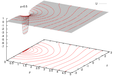
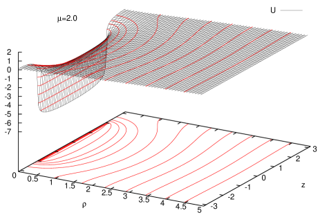
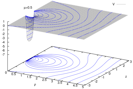
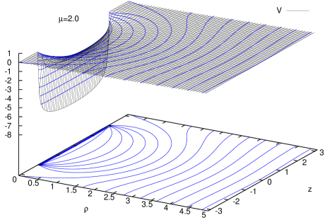
FIG. 1.: Compactified Schwarzschild black hole solutions for $\mu=0.5$ (left) and $\mu=2.0$ (right). The surface plots show the gravitational potential $U(\rho,z)$ (top) and the function $V(\rho,z)$ (bottom); red and blue contours represent equipotential surfaces of $U$ and $V$ correspondingly.

To find the gravitational potential $U(\rho,z)$ one can use either its integral representation (56) or the series (71). We used both methods. Integrals (56) were evaluated using Maple, while the series (71) were implemented in C code using FFT techniques. Both methods give results which agree with high accuracy, but of course the C implementation is much more computationally efficient. The function $V(\rho,z)$ was recovered by direct integration of differential equation (3) by finite differencing in $Z$-direction. The gravitational potential $U(\rho,z)$, function $V(\rho,z)$, and their equipotential surfaces for two different values of $\mu$ are shown in Figure 1.

IV Properties of CS black holes

         

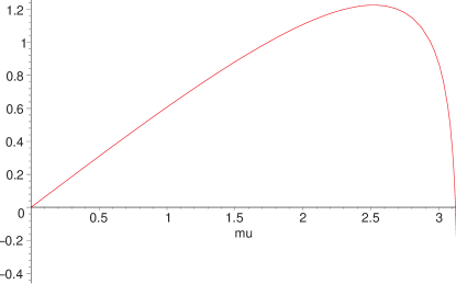
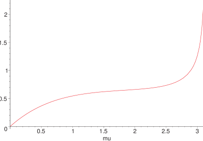
FIG. 2.: Redshift factor $u$ (left) and the irreducible mass $\mu_{0}=\mu\,\exp(-u)$ as functions of $\mu$.

A Large distance asymptotics

Let us first analyze the asymptotic behavior of the CS-metric at large distance $\rho$. For this purpose we use the integral representation (56) for $U$. It is easy to check that the integrand expression at large $\rho$ is of order of $O(\beta^{-2})$ and hence the integral is of order of $\rho^{-1}$. Thus the ln-term in the square brackets in (56) is leading at the infinity so that

$$U(\rho,z)|_{\rho\to\infty}\sim{\mu\over\pi}\ln\rho\,.$$ (86)

Using equation (3) we also get

$$V(\rho,z)|_{\rho\to\infty}\sim{\mu^{2}\over\pi^{2}}\ln\rho\,.$$ (87)

The metric (30) in the asymptotic region $\rho\to\infty$ is of the form

$$ds^{2}=-\rho^{2{\mu\over\pi}}\,dt^{2}+\rho^{-2{\mu\over\pi}(1-{\mu\over\pi})}\,(d\rho^{2}+dz^{2})+\rho^{-2{\mu\over\pi}}\,\rho^{2}\,d\phi^{2}\,.$$ (88)

The proper size of a closed Killing trajectory for the vector $\partial_{z}$ is

$$C_{z}=2\pi L\rho^{-{\mu\over\pi}(1-{\mu\over\pi})}\,.$$ (89)

The metric (88) coincides with the special case $(a_{1}=a_{2})$ of the Kasner solution [19]

$$ds^{2}=-\rho^{2a_{0}}\,dt^{2}+\rho^{2a_{1}}\,d\rho^{2}+\rho^{2a_{2}}\,dz^{2}+\rho^{2a_{3}}\,d\phi^{2}\,,$$ (90)

$$a_{1}+1=a_{2}+a_{3}+a_{0}\,,$$ (91)

$$(a_{1}+1)^{2}=a_{2}^{2}+a_{3}^{2}+a_{0}^{2}\,.$$ (92)

One can rewrite the metric (87) by using the proper-distance coordinate $l$. For small $\mu$

$$l={\rho^{1-{\mu\over\pi}}\over 1-{\mu\over\pi}}\,,$$ (93)

and the metric in the $(\rho,\phi)$-sector takes the form

$$dl^{2}+\left(1-{\mu\over\pi}\right)^{2}\,l^{2}\,d\phi^{2}\,.$$ (94)

Thus the metric of the CS black hole has an angle deficit $2\mu$ at infinity.

The asymptotic form of the metric can be used to determine the mass of the system. Let $\xi_{(t)}^{\mu}$ be a timelike Killing vector and $\Sigma$ be a 2-D surface lying inside $t$=const hypersurface, then the Komar mass $m$ is defined as

$$m={1\over 4\pi}\,\int_{\Sigma}\,\xi_{(t)}^{\mu;\nu}\,d\sigma_{\mu\nu}\,.$$ (95)

For simplicity we choose $\Sigma$ so that $t$=const and $\rho=\rho_{0}$=const. For this choice

$$d\sigma_{\mu\nu} = {1\over 2}\,\delta^{0}_{[\mu}\,\delta^{1}_{\nu]}\,\rho_{0}^{1+2a_{1}}\,dz\,d\phi\,,$$ (96)

$$\xi_{\mu;\nu} = -2a_{0}\,\rho_{0}^{2a_{0}-1}\,\delta_{[\mu}^{0}\,\delta_{\nu]}^{1}\,,$$ (97)

$$\xi^{\mu;\nu} = 2a_{0}\,\rho_{0}^{-2a_{1}-1}\,\delta^{[\mu}_{0}\,\delta^{\nu]}_{1}\,.$$ (98)

Substituting these expressions into (95) and taking the integral we get $m=\mu$. Since all our quantities are normalized by the radius of compactification $L$, we obtain that the Komar mass of our system is $M=L\mu$.

B Redshift factor, surface gravity, and proper distance between black hole poles

Using equation (80), we obtain for the redshift factor $u$ the following expression

$$u={\mu\over\pi}\ln(4\pi)+{1\over 2}\ln f(\mu)\,.$$ (99)

Figure 2(left) shows dependence of the redshift factor $u$ on parameter $\mu$. Using the approximation (83) we can write

$$u\approx{\mu\over\pi}\,\ln(4\pi)+{1\over 2}\ln\left(1-{\mu\over\pi}\right)\,.$$ (100)

The redshift factor $u$ has maximum $u_{*}$

$$u_{*}=\ln(4\pi)-{1\over 2}\left[1+\ln 2+\ln(\ln(4\pi))\right]\approx 1.22$$ (101)

at

$$\mu=\pi(1-1/(2\ln(4\pi)))\approx 2.52\,.$$ (102)

For $\mu>\mu_{*}$ the function $u$ rapidly falls down, becoming negative and logarithmically divergent at $\mu=\pi$.

In the same approximation we get the following expressions for the irreducible mass $\mu_{0}$ and the surface gravity $\kappa$

$$\mu_{0}=\mu\,\exp(-u) \approx \mu\,(4\pi)^{-{\mu\over\pi}}\,\left(1-{\mu\over\pi}\right)^{-{1\over 2}},$$ (103)

$$\kappa={e^{-2u}\over 4\mu} \approx {1\over 4\mu}\,(2\pi)^{2{\mu\over\pi}}\left(1-{\mu\over\pi}\right)\,.$$ (104)

For $\mu\to\pi$, they behave as $\mu_{0}\to\infty$ and $\kappa\to 0$. Figure 2(right) shows the irreducible mass $\mu_{0}$ as a function of $\mu$.

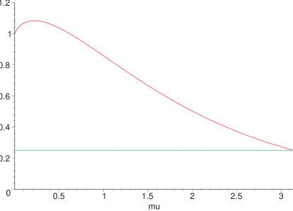
FIG. 3.: $l/(2\pi)$ as a function of $\mu$.

Another invariant characteristic of the solution is the proper distance between the ‘north pole’, $z=\mu$, and ‘south pole’, $z=-\mu$, along a geodesic connecting these poles and lying outside the black hole. This distance, $l(\mu)$, is

$$l(\mu) = 2\int\limits_{\mu}^{\pi}\,dz\,e^{-U(0,z)}$$ (105)

$$\approx 2(4\pi)^{-\mu/\pi}\,\int\limits_{\mu}^{\pi}\,dz\,\sqrt{{(z+\mu)(2\pi-z+\mu)\over(z-\mu)(2\pi-z-\mu)}}$$ (106)

$$= \textstyle 2\sqrt{\pi^{2}-\mu^{2}}\,E(\varphi,k)\,+2\mu\sqrt{{\pi+\mu\over\pi-\mu}}\,F(\varphi,k)\,-(\pi-\mu)\,,$$ (107)

where

$$\varphi=\sqrt{1-\mu/\pi}\,,\hskip 10.00002ptk={1\over\sqrt{1-(\mu/\pi)^{2}}}\,.$$ (108)

Here $F(\varphi,k)$ and $E(\varphi,k)$ are the elliptic integrals of the first and second kind, respectively. In particular one has

$$l(0)=2\pi\,,\hskip 10.00002ptl(\pi)=\pi/2\,.$$ (109)

Figure 3 shows $l/(2\pi)$ as a function of $\mu$. It might be surprising that in the limit $\mu\to\pi$, when the coordinate distance $\Delta z$ between the poles tends to 0, the proper distance between them remains finite. This happens because in the same limit the surface gravity tends to 0.

C Size and shape of the event horizon

         

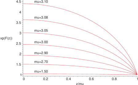
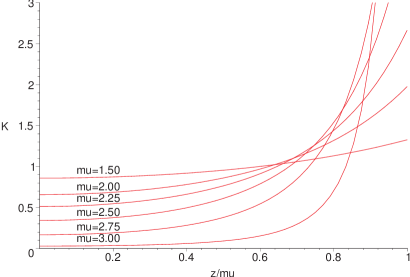
FIG. 4.: The shape function $\exp({\cal F}(z))$ (left) and the Gaussian curvature of the horizon $K(z)$ (right) for different values of $\mu$.

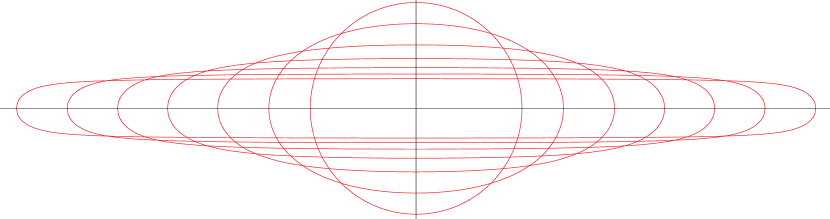
FIG. 5.: Embedding diagrams for the surface of the black hole horizon. By rotating a curve from a family shown at the plot around a horizontal axis one obtains surface isometric to the surface of a black hole described by the metric $d\sigma^{2}$. Different curves correspond to different values of $\mu$. The larger $\mu$ the more oblate is the form of the curve.

The surface area of the distorted horizon (28) written in units $L^{2}$ is

$$A=16\pi\mu_{0}^{2}\,,$$ (110)

where $\mu_{0}$ is the irreducible mass (103). The shape of the horizon is determined by the shape function

$${\cal F}(z)=\hat{U}(z)-u\,.$$ (111)

Figure 4(left) shows a plot of $\exp({\cal F}(z))$ for several values of $\mu$. By multiplying the 2-metric on the horizon $d\gamma^{2}$ by $(2\mu_{0})^{-2}$ one obtains the metric of the 2-surface which has the topology of a sphere $S^{2}$ and the surface area $4\pi$. The metric describing this distorted sphere is

$$d\sigma^{2}=e^{2{\cal F}}{dz^{2}\over\mu^{2}-z^{2}}+e^{-2{\cal F}}(\mu^{2}-z^{2}){d\phi^{2}\over\mu^{2}}\,.$$ (112)

The Gaussian curvature of the metric $d\sigma^{2}$ is $K={1\over 2}R$, where $R$ is the Ricci scalar curvature. It is given by the following expression

$$K=e^{-2{\cal F}(z)}\,\left[1+(\mu^{2}-z^{2})\,[{\cal F}^{\prime\prime}-2({\cal F}^{\prime})^{2}]\,-4z{\cal F}^{\prime}\right]\,.$$ (113)

The Gauss-Bonnet formula gives

$$\int d^{2}x\,\sqrt{\sigma}\,K=4\pi\,.$$ (114)

For the unperturbed black hole $K=1$. As a result of deformation, the CS-black hole has $K>1$ at the poles, $z=\pm\mu$, and $K<1$ at the ‘equatorial plane’, $z=0$. Figure 4(right), which shows $K(z)$ for different values of $\mu$, illustrates this feature. This kind of behavior can be easily understood as a result of self-attraction of the black hole because of the compactification of the coordinate $z$.

Using approximation (83) allows one to obtain simple analytical expressions for the shape function and the Gaussian curvature. Equations (80) and (99) give

$${\cal F}={1\over 2}\,\ln\left[{f({\mu+z\over 2})f({\mu-z\over 2})\over f(\mu)}\right]\approx{1\over 2}\,\ln\left[1+{\mu^{2}-z^{2}\over 4\pi(\pi-\mu)}\right]\,.$$ (115)

Let us write the metric $d\sigma^{2}$ in the form

$$d\sigma^{2}=F(z)\,dz^{2}+{d\phi^{2}\over\mu^{2}\,F(z)}\,,$$ (116)

then in this approximation one has

$$F(z)\approx{1\over\mu^{2}-z^{2}}+{1\over 4\pi^{2}(1-\mu/\pi)}\,.$$ (117)

while the Gaussian curvature is

$$K\approx{16\pi^{2}(\pi-\mu)^{2}[(2\pi-\mu)^{2}+3z^{2}]\over[(2\pi-\mu)^{2}-z^{2}]^{3}}\,.$$ (118)

The Gaussian curvature is positive in the interval $|z|<\mu$.

It is interesting to note that the horizon geometry of the CS-black hole coincides (up to a constant factor) with the geometry on the 2-D surface of the horizon of the Euclidean 4-D Kerr black hole. This fact can be easily checked since the induced 2-D geometry of the horizon of the Kerr black hole is (see e.g. equation 3.5.4 in [18])

$$dl^{2}=(r_{+}^{2}+a^{2})\,\left[\tilde{F}(x)\,dx^{2}+\frac{d\phi^{2}}{\tilde{F}(x)}\right],$$ (119)

where

$$\tilde{F}(x)=\frac{1}{1-x^{2}}-\beta^{2}\,,\hskip 10.00002pt\beta=\frac{a}{\sqrt{r_{+}^{2}+a^{2}}}\,.$$ (120)

Here $r_{+}=M+\sqrt{M^{2}-a^{2}}$ gives the position of the event horizon, and $M$ and $a$ are the mass and the rotation parameter of the Kerr black hole. The line element (116,117) is obtained from the above by coordinate redefinition $z=\mu x$ and analytic continuation $\alpha=i\beta$, with $\alpha=\frac{\mu}{2\pi}(1-\frac{\mu}{\pi})^{-\frac{1}{2}}$.

Denote by $l_{\text{eq}}$ the proper length of the equatorial circumference, and by $l_{\text{pole}}$ the proper length of a closed geodesic passing through both poles $|z|=\mu$ of the black hole horizon. Then one has

$$l_{\text{eq}}(\mu) \approx 2\pi\,{\sqrt{1-\mu/\pi}\over 1-\mu/(2\pi)}\,,$$ (121)

$$l_{\text{pole}}(\mu) \approx 4E\left({i\mu\over 2\pi\sqrt{1-\mu/\pi}}\right)\,,$$ (122)

where $E(k)$ is the complete elliptic integral of the second kind. One has $l_{\text{eq}}(0)=l_{\text{pole}}(0)=2\pi$ and the surface is a round sphere. For $\mu\to\pi$ the lengths $l_{\text{eq}}\to 0$ and $l_{\text{pole}}\to\infty$.

D Embedding diagrams for a distorted horizon

The metric (116) can be obtained as an induced geometry on a surface of rotation $\Sigma$ embedded in a 3 dimensional Euclidean space. Let

$$dl^{2}=dh^{2}+dr^{2}+r^{2}\,d\phi^{2}\,$$ (123)

be the metric of the Euclidean space and the surface $\Sigma$ be determined by an equation $h=h(r)$, then the induced metric on $\Sigma$ is

$$d\sigma^{2}=\left[1+\left({dh\over dr}\right)^{2}\right]\,dr^{2}+r^{2}\,d\phi^{2}\,.$$ (124)

By comparing this metric with (116) we get

$$r={1\over\sqrt{F(z)}}\,,$$ (125)

$$\left({dh\over dz}\right)^{2}+\left({dr\over dz}\right)^{2}=F(z)\,.$$ (126)

These equations imply the following differential equation for $h(z)$

$${dh\over dz}=\sqrt{F-{{F^{\prime}}^{2}\over 4F^{3}}}\,.$$ (127)

Figure 5 shows the embedding diagrams for the distorted horizon surfaces of a compactified black hole for different values of $\mu$. The larger is the value $\mu$ the more oblate is the surface of the horizon. For large $\mu$ close to $\pi$ it has a cigar-like form.

E $\mu\to\pi$ limit

Let us now discuss the properties of the spacetime in the limiting case $\mu\to\pi$. This limit can be easily taken in the series representation (71) for the gravitational potential $U$. Since $\sin(\pi k)=0$ for $k>0$, only the logarithmic term survives in this limit. Thus $U(\rho,z)=\ln\rho$. Since the limiting metric is invariant under translations in $z$-direction, it has the form of the Kasner solution (88) with $\mu=\pi$ and reads

$$ds^{2}=-\rho^{2}\,dt^{2}+d\rho^{2}+dz^{2}+d\phi^{2}\,.$$ (128)

This is a Rindler metric with two dimensions orthogonal to the acceleration direction being compactified

$$z\in(-\pi,\pi)\,,\hskip 10.00002pt\phi\in(-\pi,\pi)\,.$$ (129)

Restoring the dimensionality we can write this metric as

$$dS^{2}=-{R^{2}\over L^{2}}\,dT^{2}+dR^{2}+dZ^{2}+L^{2}d\phi^{2}\,.$$ (130)

V Discussion

The obtained results can be summarized as follows. If the size of a black hole is much smaller that the size of compactification, its distortion is small. The deformation which makes the horizon prolated grows with the black hole mass. For large mass $\mu\geq\pi/2$ the black hole deformation becomes profound. The pole parts of the horizon, that is parts close to $z=-\mu$ and $z=\mu$, attract one another. As a result of this attraction the Gaussian curvature of regions close to black hole poles grows, while the Gaussian curvature in the ‘equatorial’ region falls down and the surface of the horizon is ‘flattened down’ in this region. For large value of the mass $\mu$, the ‘flattening’ effects occurs for a wide range of the parameter $z$. Such a black hole reminds a cigar or a part of the cylinder with two sharpened ends.

We did not include any branes in our consideration. However, we should note that the surface $Z=0$ is a solution of the Nambu-Goto action for a test brane. This can be easily seen, as the solution we discussed is symmetric around the surface $Z=0$, which implies that its extrinsic curvature vanishes there. At far distances the induced gravitational field on the $Z=0$ submanifold is asymptotically a solution of vacuum $(2+1)$-dimensional Einstein equations. It is not so for regions close to the black hole. This “violation” of the vacuum $(2+1)$-dimensional Einstein equations for the induced metric makes the existence of the $(2+1)$-dimensional black hole on the brane possible.

In our work we did not find any indications on instability of a black hole which might be interpreted as connected with the Gregory-Laflamme instability [22, 23]. It may not be surprising since these kind of instabilities are expected in spacetimes with higher number of dimensions (see e.g. [21, 24, 25, 26]).

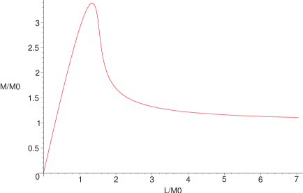
FIG. 6.: $M$ as a function of $L$ for fixed $M_{0}$.

On the other hand, a solution describing a black hole in a compactified spacetime may be unstable for a different reason. The nature of this instability is the following. In our set-up we fix a radius of compactification $L$. In a flat spacetime we can choose parameter $L$ arbitrarily and the energy of the system, being equal to zero, does not depend on this choice. The situation is different in the presence of a black hole. Consider a black hole of a given area, that is with a fixed parameter $M_{0}$. Since the black hole entropy, which is proportional to the area, remains unchanged for quasi-stationary adiabatic processes, one may consider different states of a black hole with a given $M_{0}$. $L$ plays a role of an independent parameter, specifying a solution. In particular one has

$$M_{0}={M\,(4\pi)^{-M/(\pi L)}\over\sqrt{1-M/(\pi L)}}\,.$$ (131)

This relation shows that for fixed $M_{0}$ the energy of the system $M$ depends on compactification radius $L$. The plot of the function $M(L)$ is shown at Figure 6. For $L=L_{*}=1.345M_{0}$ the mass $M$ has maximum $M=M_{*}=3.3877M_{0}$. At the corresponding value $\mu_{*}=2.52$ the function $u(\mu)$ has its maximum. Thus if one starts with a system with $L>L_{*}$ then a positive variation of parameter $L$ will decrease the energy of the system. In this case the lowest energy state corresponds to $L\to\infty$, so that a stable solution will be an isolated Schwarzschild black hole in an empty spacetime without any compactifications. In the opposite case, $L<L_{*}$, the energy decreases when $L\to 0$. In this limit $M\approx\pi L$ and hence it corresponds to a limiting solution $\mu\to\pi$. The limiting metric is given by (130). The corresponding spacetime is a 2-D torus compactification of the Rindler metric.

This argument, based on the energy consideration, indicates a possible instability of a compactified spacetime with a black hole with respect to compactified dimension either ‘unwrapping’ completely or being ‘swallowed’ by a black hole. While ‘unwrapping’ of the extra dimension may be prevented by the usual stabilization mechanisms, the other instability regime might not be so benign. It is interesting to check whether this conjecture is correct by standard perturbation analysis.

REFERENCES

- [1] G. W. Gibbons and D. L. Wiltshire, Black holes in Kaluza-Klein theory, Annals Phys. 167, 201 (1986) [Erratum-ibid. 176, 393 (1987)].
- [2] F. Larsen, Kaluza-Klein black holes in string theory, hep-th/0002166.
- [3] R. C. Myers, Higher dimensional black holes in compactified space-times, Phys. Rev. D 35, 455 (1987).
- [4] A. Chamblin, S. W. Hawking and H. S. Reall, Brane-world black holes, Phys. Rev. D 61, 065007 (2000) [hep-th/9909205].
- [5] R. Emparan, G. T. Horowitz and R. C. Myers, Exact description of black holes on branes, JHEP 0001, 007 (2000) [hep-th/9911043].
- [6] H. Kudoh, T. Tanaka and T. Nakamura, Small localized black holes in braneworld: Formulation and numerical method, gr-qc/0301089.
- [7] N. Arkani-Hamed, S. Dimopoulos and G. R. Dvali, The hierarchy problem and new dimensions at a millimeter, Phys. Lett. B 429, 263 (1998) [hep-ph/9803315].
- [8] A. R. Bogojevic and L. Perivolaropoulos, Black holes in a periodic universe, Mod. Phys. Lett. A 6, 369 (1991).
- [9] T. Harmark and N. A. Obers, Black holes on cylinders, JHEP 0205, 032 (2002) [hep-th/0204047].
- [10] W. Israel and K. A. Khan, Collinear particles and Bondi dipoles in General Relativity, Nouvo Cimento 33, 331 (1964).
- [11] D. Korotkin and H. Nicolai, A periodic analog of the Schwarzschild solution, gr-qc/9403029.
- [12] R. Geroch and J. B. Hartle, Distorted black holes, J. Math. Phys. 23 680 (1981).
- [13] S. Fairhurst and B. Krishnan, Distorted black holes with charge, Int. J. Mod. Phys. D 10, 691 (2001) [gr-qc/0010088].
- [14] S. S. Yazadjiev, Distorted charged dilaton black holes, Class. Quant. Grav. 18, 2105 (2001) [gr-qc/0012009].
- [15] R. Emparan and H. S. Reall, Generalized Weyl solutions, Phys. Rev. D 65, 084025 (2002) [hep-th/0110258].
- [16] T. Shiromizu and M. Shibata, Black holes in the brane world: Time symmetric initial data, Phys. Rev. D 62, 127502 (2000) [hep-th/0007203].
- [17] E. Sorkin and T. Piran, Initial data for black holes and black strings in 5d, hep-th/0211210.
- [18] V. P. Frolov and I. D. Novikov, Black hole physics: Basic concepts and new developments, Kluwer Academic Publ. (1998).
- [19] E. Kasner, Geometrical theorems on Einstein’s cosmological equations, Am. J. Math. 43 217 (1921).
- [20] A. P. Prudnikov, Yu. A. Brychkov, and O. I. Marichev, Integrals and series v.I, Gordon and Breach Science Publishers (1986).
- [21] R. Gregory and R. Laflamme, Hypercylindrical black holes, Phys. Rev. D 37, 305 (1988).
- [22] R. Gregory and R. Laflamme, Black strings and p-branes are unstable, Phys. Rev. Lett. 70, 2837 (1993) [hep-th/9301052].
- [23] R. Gregory and R. Laflamme, The Instability of charged black strings and p-branes, Nucl. Phys. B 428, 399 (1994) [hep-th/9404071].
- [24] B. Kol, Topology change in general relativity and the black-hole black-string transition, hep-th/0206220.
- [25] T. Wiseman, From black strings to black holes, Class. Quant. Grav. 20, 1177 (2003) [hep-th/0211028].
- [26] T. Wiseman, Static axisymmetric vacuum solutions and non-uniform black strings, Class. Quant. Grav. 20, 1137 (2003) [hep-th/0209051].