hep-th/0302050
BROWN-HET-1341

A note on $\alpha$-vacua and interacting field theory in de Sitter space
Kevin Goldstein and David A. Lowe

Department of Physics,
Brown University,
Providence, RI 02912, USA.

Using an imaginary time formalism, we set up a consistent renormalizable perturbation theory of a scalar field in a nontrivial $\alpha$ vacuum in de Sitter space. Although one representation of the effective action involves non-local interactions between anti-podal points, we argue the theory leads to causal physics when continued to real-time, and we prove a spectral theorem for the interacting two-point function. We construct the renormalized stress energy tensor and show this develops no imaginary part at leading order in the interactions, consistent with stability.

1 Introduction

A common problem in formulating quantum field theory on a curved background is ambiguity in the choice of vacuum. In de Sitter space there is a one-parameter family of vacua invariant under the de Sitter group, which have been dubbed the $\alpha$ vacua [1, 2, 3, 4]. These vacua are perfectly self-consistent in the context of free theories. It has long been suggested that the only physically sensible vacuum is the Euclidean (a.k.a. Bunch-Davies) vacuum.

One reason for this choice is that the free propagators in the Euclidean vacuum exhibit a Hadamard singularity, which matches with what is expected in the flat space limit [5, 6]. However the physical motivation for restriction to Hadamard singular propagators is obscure in the context of interacting quantum field theory, and certainly nothing appears to go wrong with the $\alpha$-vacuum propagators at the free level. In particular, as shown in [4] the commutator Green function is vanishing at spacelike separations in an $\alpha$-vacuum and in fact is independent of $\alpha$.

The Green functions in a nontrivial $\alpha$ vacuum exhibit singular correlations between anti-podal points. Of course since the commutator is compatible with locality this does not lead to acausal propagation of information. However some authors have suggested that once interactions are included the $\alpha$-vacua do not lead to a sensible perturbative expansion of Green functions. Banks et al. [7] have argued non-local counter-terms render the effective action inconsistent. Einhorn et al. [8] have argued that $\alpha$ vacuum correlation functions are non-analytic and conclude that they are physically unacceptable. Related arguments are made in Kaloper et al. [9], who argue that because an Unruh detector is not in thermal equilibrium in an $\alpha$ vacuum, thermalization will lead to decay to a Euclidean vacuum.

This issue has direct bearing on the theory of inflation. The conventional view of inflation places the inflaton in the Euclidean vacuum. However, as emphasized in [10, 11, 12] , the initial conditions for inflation may place the inflaton in a non-trivial $\alpha$-vacuum, see also [13] for earlier work in this direction. This has a potentially large effect on the predictions for the CMB spectrum, see for example [10, 11, 12, 14] and references therein. Furthermore, if there is a residual value of $\alpha$ today, there are many interesting predictions for other observable quantities such as cosmic rays, that we consider in more detail in [15].

In this paper we show in an imaginary time formulation the $\alpha$-vacua do indeed have a well-defined perturbative expansion, that yields finite renormalized amplitudes in a conventional manner. This goes a long way to refuting some of the objections raised in [7, 8, 9], see also [16] for discussion of consistency of $\alpha$-vacua.

We begin in section 2 by reviewing the free field results of [1, 2, 3, 4]. In particular, the $\alpha$-vacuum may be regarded as a squeezed state created by a unitary operator $U$ acting on the Euclidean vacuum. This idea will be central to the formalism we develop. This leads to a generalized Wick’s theorem, which allows us to expand any free $\alpha$-vacuum Green function in terms of products of Euclidean vacuum two-point functions. In section 3 we describe the interacting theory in an imaginary time formalism. In particular, in interaction picture, we show the effective Lagrangian becomes non-local when $U$ is commuted through the fields. We show that UV divergences in amplitudes satisfy a non-trivial factorization relation which relates the coefficients of local counter-terms to non-local ones. Once local counter-terms are fixed, non-local terms are completely determined, which implies the theory is renormalizable in the conventional sense. In section 4 we outline how to continue the imaginary time amplitudes to real time. We carry this through in detail for the interacting two-point function, and prove a spectral theorem in this case. One immediate consequence is that even in the interacting theory, the expectation value in an $\alpha$-vacuum of the commutator of two fields vanishes at spacelike separations, as required for causality of local observables. In section 5 we use the Green function to define a renormalized stress energy tensor, and we conclude in section 6.

2 Free fields

Let us begin by reviewing the construction of the $\alpha$-vacua [4, 3, 1, 2]. We will set the Hubble radius $1/H=1$ unless otherwise stated. In general a free scalar field has the mode expansion

$$\phi(x)=\sum_{n}a_{n}\phi_{n}(x)+a_{n}^{\dagger}\phi^{*}_{n}(x)$$ (1)

where $\{\phi_{n}\}$ satisfy the Klein-Gordon equation and $[a_{n},a^{\dagger}_{m}]=\delta_{nm}$. The $\phi_{n}$ are complete and orthonormal with respect to the Klein-Gordon product

$$(\phi_{1}(x),\phi_{2}(x))=-i\int_{\Sigma}(\phi_{1}\partial_{\mu}\phi_{2}^{*}-\phi_{2}^{*}\partial_{\mu}\phi_{1})d\Sigma^{\mu}$$ (2)

with $\Sigma$ a spacelike slice. In this paper we consider scalars with mass $m$ and $R\phi^{2}$ coupling $\xi$. In a fixed de Sitter background we can absorb $\xi$ into a redefinition of $m$, so we drop $\xi$ from now on.

The vacuum state is characterized by

$$a_{n}|\Omega_{a}\rangle=0~{}.$$ (3)

In general we can expand in another set of modes

$$\phi(x)=\sum_{n}b_{n}\phi_{n}^{\alpha}(x)+b_{n}^{\dagger}{\phi^{\alpha}_{n}}^{*}(x)$$ (4)

related to the first by a Bogoliubov transformation. A new vacuum state is defined by

$$b_{n}|\Omega_{b}\rangle=0~{}.$$ (5)

As mentioned in dS space there is a one complex-parameter family of the dS invariant vacua, dubbed the alpha vacua, $|\alpha\rangle$. One of these, the Euclidean or Bunch-Davies vacuum, $|E\rangle$, is defined by using mode functions obtained by analytically continuing mode functions regular on the lower half of the Euclidean sphere. The Euclidean modes can be chosen such that $\phi^{E}_{n}(x)^{*}=\phi^{E}_{n}(\bar{x})$, where $\bar{x}$ is the antipode of $x$, ($\bar{x}\equiv-x$). See, for example, [3, 17] for explicit expressions of these mode functions.

The modes of an arbitrary $\alpha$-vacuum general are related to the Euclidean ones by a mode number independent Bogoliubov transformation,

$$\phi^{\alpha}_{n}=N_{\alpha}(\phi^{E}_{n}+e^{\alpha}{\phi_{n}^{E}}^{*})$$ (6)

where $N_{\alpha}\equiv(1-\exp(\alpha+\alpha^{*}))^{-\frac{1}{2}}$ and we require that ${\rm Re}(\alpha)<0$. The Euclidean vacuum corresponds to $\alpha=-\infty$.

In terms of creation and annihilation operators

$$b_{n}=N_{\alpha}(a_{n}-e^{\alpha*}{a_{n}^{\dagger}})$$ (7)

where $b$ and $a$ are operators satisfying (3) with respect to the $\alpha$-vacuum and Euclidean respectively. This transformation can be implemented using a unitary operator

$$b_{n}={\cal U}a_{n}{\cal U}^{\dagger}$$ (8)

where

$${\cal U}_{\alpha}\equiv\exp(\sum_{n}c_{\alpha}{a^{\dagger}_{n}}^{2}-c^{*}_{\alpha}a_{n}^{2})$$ (9)

$$c_{\alpha}\equiv\frac{1}{4}\exp(-i{\rm Im}(\alpha))\log\tanh(-{\rm Re}(\alpha)/2)$$ (10)

and we use the standard Taylor expansion of the exponential to define the ordering. The vacua are related by

$$|\alpha\rangle={\cal U}_{\alpha}|E\rangle$$ (11)

since

$$b_{n}{\cal U}|E\rangle={\cal U}a_{n}|E\rangle=0~{}.$$ (12)

From this perspective the $\alpha$-vacuum may be viewed as a squeezed state on top of the usual Euclidean vacuum.

2.1 Generalized Wick’s theorem

The Fock space built on the $\alpha$ vacuum is not unitary equivalent to that of the Euclidean vacuum in general, because the unitary transformation mixes positive and negative frequencies. However, as far as quantum field theory in a fixed de Sitter background goes, this unitary transformation leaves the complete set of physical observables invariant. For our purposes, we take these observables to be finite time Green functions, from which one may obtain $S$-matrix elements as described in [18, 19]. All this unitary transformation does is to mix these observables up in a non-local way, as we explain in more detail later in this section. This is the underlying reason that the interacting $\alpha$-vacuum theory is consistent.

If we were only considering the $\phi$ field on its own this would be the end of the story. However if we wish to view $\phi$ as the inflaton, physics dictates that $\phi$ should be locally coupled to other fields. Thus we are interested in correlators of the field $\phi$ with respect to the $\alpha$ vacuum. The conjugated field ${\cal U}\phi(x){\cal U}^{\dagger}$ on the other hand, would yield correlators in the $\alpha$-vacuum identical to the usual Euclidean vacuum correlators of $\phi$, but would be coupled non-locally to other fields.

Since the unitary transformation involves modes of arbitrarily high frequency (up to some physical cutoff) the systematics of renormalizable perturbation theory will be quite different from the usual Euclidean vacuum perturbation theory [20, 21, 22, 23, 24, 25]. It will be our goal in the rest of this paper to elaborate on renormalizable perturbation theory in the $\alpha$-vacuum.

The correlators of interest take the form of expectation values of products of fields $\phi$ with respect to the state $|\alpha\rangle$, or equivalently as conjugated fields $\tilde{\phi}\equiv{\cal U}^{\dagger}\phi{\cal U}$ with respect to $|E\rangle$

$$\begin{array}[]{lcl}\langle\alpha|\phi(x_{1})\phi(x_{2})\ldots\phi(x_{n})|\alpha\rangle&=&\langle E|{\cal U}^{\dagger}\phi(x_{1}){\cal U}{\cal U}^{\dagger}\phi(x_{2}){\cal U}{\cal U}^{\dagger}\ldots{\cal U}{\cal U}^{\dagger}\phi(x_{n}){\cal U}|E\rangle\\ &=&\langle E|\tilde{\phi}(x_{1})\tilde{\phi}(x_{2})\ldots\tilde{\phi}(x_{n})|E\rangle~{}.\end{array}$$ (13)

Now, letting $\gamma=e^{\alpha}$ (so that $|\gamma|<1$),

$$\begin{array}[]{ll}\tilde{\phi}(x)&={\cal U}^{\dagger}\phi(x){\cal U}\\ &={\cal U}^{\dagger}\left({\displaystyle\sum_{n}}\phi^{\alpha}_{n}(x)b_{n}+\phi_{n}^{\alpha*}(x)b_{n}^{\dagger}\right){\cal U}\\ &={\displaystyle\sum_{n}}\phi^{\alpha}_{n}(x)a_{n}+\phi_{n}^{\alpha*}(x)a_{n}^{\dagger}\\ &=N_{\alpha}{\displaystyle\sum_{n}}\left(\phi^{E}_{n}(x)+\gamma{\phi_{n}^{E}}(\bar{x})\right)a_{n}+\left({\phi^{E}_{n}}(x)+\gamma{\phi_{n}^{E}}(\bar{x})\right)^{*}a_{n}^{\dagger}\\ &=N_{\alpha}\left(\phi_{0}(x)+\phi_{1}(x)\right)\end{array}$$ (14)

where we have defined

$$\phi_{0}(x)\equiv\phi(x)~{},\qquad\phi_{1}(x)\equiv\sum_{n}\gamma\phi_{n}^{E}(\bar{x})a_{n}+\gamma^{*}{\phi_{n}^{E}}^{*}(\bar{x})a_{n}^{\dagger}$$ (15)

If $\gamma$ is real, then $\tilde{\phi}(x)$ is simply a linear combination of $\phi(x)$ and $\phi(\bar{x})$. For $\gamma$ complex this isn’t quite true, but the additional phases are simple to keep track of.

Using these relations we can express any $\alpha$-vacuum correlator in terms of a sum of Euclidean vacuum correlators, giving us a generalized Wick’s theorem. The simplest example is

$$\begin{array}[]{lll}\langle\alpha|\phi(x)\phi(y)|\alpha\rangle&=&N_{\alpha}^{2}\left(G_{E}(x,y)+|\gamma|^{2}G_{E}(\bar{x},\bar{y})+\gamma G_{E}(\bar{x},y)+\gamma^{*}G_{E}(x,\bar{y})\right)\\ &\equiv&G_{\alpha}(x,y)\end{array}$$ (16)

where $G_{E}(x,y)\equiv\langle E|\phi(x)\phi(y)|E\rangle$ is the Wightman function on the Euclidean vacuum. It is convenient to introduce a two index notation,

$$G_{\alpha}(x,y)=\sum_{i,j=0,1}G_{ij}(x,y)$$ (17)

where

$$\begin{matrix}G_{00}(x,y)&=&N_{\alpha}^{2}G_{E}(x,y)~{},\qquad&G_{10}(x,y)&=&N_{\alpha}^{2}\gamma G_{E}(\bar{x},y)~{},\cr G_{01}(x,y)&=&N_{\alpha}^{2}\gamma^{*}G_{E}(x,\bar{y})~{},\qquad&G_{11}(x,y)&=&N_{\alpha}^{2}|\gamma|^{2}G_{E}(\bar{x},\bar{y})\cr\end{matrix}$$ (18)

which we will use later.

The Wightman function diverges when $x$ and $y$ are null separated. As we can see from (16), for the $\alpha$-vacua, there are additional divergences when one point is null separated with the antipode of another. This feature has led many to consider the $\alpha$-vacua unphysical [8, 7, 9].

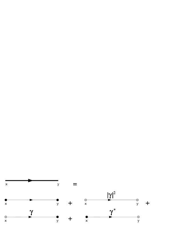
Figure 1: Feynman diagram for (16). The thick line represents the $\alpha$-vacuum propagator $G_{\alpha}(x,y)$. Thin lines represent Euclidean vacuum propagators with a factor of $N_{\alpha}^{2}$, and the other factors are shown explicitly. Grey dots denote points that appear in propagators as antipodes. We have defined $\gamma=e^{\alpha}$.

Any correlation function of the form (13) in the free theory can be found in terms of products of Green’s functions by normal-ordering the creation and annihilation operators, and retaining the fully contracted terms. For example,

$$\begin{array}[]{lll}\langle\alpha|\phi(x)\phi(y)\phi(z)\phi(w)|\alpha\rangle\\ =G_{\alpha}(x,y)G_{\alpha}(z,w)+G_{\alpha}(x,z)G_{\alpha}(y,w)+G_{\alpha}(x,w)G_{\alpha}(y,z)\\ \end{array}$$ (19)

where we have in mind using (16) to expand in terms of the Euclidean vacuum Green’s functions. Note it is important the ordering of the arguments of the Green’s functions is inherited from the ordering in the operator expression on the left-hand side. This is because we are stating the generalized Wick’s theorem in the form of Wightman functions rather than the usual form with time-ordered Green’s functions [26]. The expansion of operator products in free field theory using Wightman functions actually predates Wick’s theorem [27]. The theorem may be extended to time-ordered expectation values by replacing the Wightman functions with time-ordered two-point functions.

To convert some diagram written in terms of the $G_{\alpha}$’s into one in terms of Euclidean propagators, replace each thick line with a sum of 4 thin ones. To find the coefficient of each term just count up the number of grey dots, noting their orientation with respect to the arrows. This is written more compactly using the two index notation (17), with an index $i=0,1$ appearing at the end of each propagator, and all indices summed over.

3 Interacting fields

So far all we have said is valid regardless of whether we work on de Sitter space, or its Euclidean continuation, the four-sphere. Once we introduce interactions, however, the choice of Lorentzian versus Euclidean signature has a major impact on the formalism used to setup the perturbative expansion. This is familiar from finite temperature field theory where one has an imaginary time formalism [28, 29] or alternatively one can use a formulation in terms of real time propagators at the price of doubling the number of fields [30, 31].

Describing interacting fields in curved spacetime with event horizons using Lorentzian signature formalism is problematic. Inevitably one must deal with propagators on opposite sides of the horizon, and this leads to ambiguities in the formulation of Feynman rules. The same problem exists for spacetimes with cosmological horizons, as would arise if one attempted to quantize a field in de Sitter space in the static coordinate patch. To avoid these issues we formulate interacting field theory using the imaginary time, or Euclidean continuation, as advocated in [32]. Eventually we have in mind defining real-time ordered correlators which may be used to construct in-out $S$-matrix elements as described in [18, 19].

In the Euclidean vacuum, this problem has been much studied in the literature [20, 21, 22, 23, 24, 25, 33] and corresponds to doing field theory on $S^{4}$. Our strategy will be to use (11) to define the interacting $\alpha$-vacuum, and construct physical observables as correlators of the field $\phi$ which couple locally to physical sources. To evaluate these observables we set up the perturbation theory on the Euclidean sphere as a non-local field theory in terms of $\tilde{\phi}={\cal U}^{\dagger}\phi(x){\cal U}$. We define these fields as interaction picture fields, and will work with the standard methods of canonical quantization.

The interacting part of the non-local action for $\tilde{\phi}$ is obtained by conjugating the local bare interaction terms written in terms of the $\phi$ fields with the operator $U$, or more precisely

$$T_{\tau}e^{iS_{non-local}^{int}(\tilde{\phi})}\equiv{\cal U}^{\dagger}T_{\tau}e^{iS_{local}^{int}(\phi)}{\cal U}$$ (20)

where $T_{\tau}$ denotes imaginary time ordering. The actions are obtained by integrating the lagrangian density describing the interactions (which we assume to be polynomial in $\phi$) over the Euclidean sphere. We note that when (14) is substituted into this expression, the anti-podal components $\phi_{1}(x)$ are to be ordered according to $x$ rather than $\bar{x}$, since the ordering is to be inherited from the right-hand side of (20). The determination of any correlation function of $\phi$’s in an $\alpha$-vacuum then reduces to a standard Euclidean vacuum correlator computation, albeit with some terms involving fields with unconventional time ordering. That is, we expand (20) perturbatively in the interactions, generating a sum of correlators of $\tilde{\phi}$ with respect to the Euclidean vacuum. These may then be evaluated using the generalized Wick’s theorem of the previous section.

Working on the Euclidean sphere has the advantage that a wide range of sensible cutoffs are available. For example one can choose dimensional regularization as in [22, 23, 24, 25], or simply a mode cutoff corresponding to a cutoff on angular momentum on the 4-sphere. Pauli-Villars is another option, as is point-splitting (with spherically symmetric averaging assumed to restore the symmetries), or zeta-function regularization [19, 34, 35]. Little of what we say in the present work is dependent on a particular choice of cut-off.

Let us comment further on the form of the correlators. The normalized Green functions in the $\alpha$-vacuum take the form

$$G(x_{1},\cdots,x_{n}) = \frac{\langle{\cal U}^{\dagger}T_{\tau}\phi(x_{1})\cdots\phi(x_{n})e^{iS^{int}_{local}(\phi)}{\cal U}\rangle}{\langle{\cal U}^{\dagger}T_{\tau}e^{iS^{int}_{local}(\phi)}{\cal U}\rangle}$$ (21)

$$= \frac{\langle T_{\tau}\tilde{\phi}(x_{1})\cdots\tilde{\phi}(x_{n})e^{iS^{int}_{non-local}(\tilde{\phi})}\rangle}{\langle T_{\tau}e^{iS^{int}_{non-local}(\tilde{\phi})}\rangle}~{}.$$

In imaginary time we cannot take an asymptotic limit where interactions turn off, which is important in the usual definition of the $S$-matrix to obtain the interacting vacuum. Instead we will simply compute correlators with respect to the free vacuum as in (21). As usual the denominator in (21) implies we drop disconnected diagrams when we compute Green functions. Because we are not taking an LSZ type limit, the relevant Green functions correspond to unamputated diagrams. We discuss continuation to real-time amplitudes in the next section.

Figure 2: Feynman diagram for propagator in $\lambda\phi^{3}$. The indices $i_{k}$ label end-points of the propagators $G_{ij}$. All indices are to be summed over. Vertex factors carry no $i_{k}$ dependence.

Let us now go through an example to illustrate the renormalization of mass in $\lambda\phi^{3}$. The relevant Feynman diagram in position space is shown in (2). The vertex $V_{ijk}=1$ for all $i,j,k$, so the amplitude is

$$A=\sum_{\{i_{k}=0,1\}}\int\sqrt{{\rm det}g_{\mu\nu}(w)}dw\sqrt{{\rm det}g_{\mu\nu}(z)}dzG^{F}_{i_{1}i_{2}}(x,w)G^{F}_{i_{3}i_{4}}(w,z)G^{F}_{i_{5},i_{6}}(w,z)G^{F}_{i_{7}i_{8}}(z,y)$$ (22)

where $G^{F}$ is the time-ordered Green function

$$G^{F}(x,y)=\theta(x^{0}-y^{0})G_{\alpha}(x,y)+\theta(y^{0}-x^{0})G_{\alpha}(y,x)~{},$$ (23)

and $x^{0}$ is the imaginary time coordinate on the sphere. UV divergences arise when $w\to z$ or $w\to\bar{z}$. In these limits the propagator has the form

$$\lim_{w\to z}G^{F}(w,z)=N_{\alpha}^{2}(1+|\gamma|^{2})\frac{1}{(w-z)^{2}}~{},\qquad\lim_{w\to\bar{z}}G^{F}(w,z)=N_{\alpha}^{2}(\gamma+\gamma^{*})\frac{1}{(w-\bar{z})^{2}}$$ (24)

in locally Minkowski coordinates. The UV divergent part of the amplitude is then

$$A_{UV}=\frac{\delta m^{2}}{2}\int\sqrt{{\rm det}g_{\mu\nu}(z)}dz\langle{\cal U}^{\dagger}\phi(x)\phi(z)^{2}\phi(y){\cal U}\rangle$$ (25)

where $\delta m^{2}$ is the cutoff dependent counter-term. If we adopt a simple point-splitting regularization, this is given by

$$\delta m^{2} = \left(\int_{|w-z|\geq\varepsilon}+\int_{|w-\bar{z}|\geq\varepsilon}\right)\sqrt{{\rm det}g_{\mu\nu}(w)}dw\sum_{i_{k}}G_{i_{3}i_{4}}(w,z)G_{i_{5}i_{6}}(w,z)$$ (26)

$$\propto N_{\alpha}^{4}\left((1+|\gamma|^{2})^{2}+(\gamma+\gamma^{*})^{2}\right)\log\varepsilon~{}.$$

We conclude therefore that the counter-term is indeed simply a local mass counter-term when expressed in terms of $\phi$ variables, but appears non-local when written in terms of $\tilde{\phi}$ variables.

It is perhaps worthwhile to highlight the difference between our computation and a similar computation of [7]. Reference [7] assumed the basic vertex was local. However in our formulation of the $\alpha$-vacuum field theory, the vertex takes the form ${\cal U}^{\dagger}\phi(z)^{3}{\cal U}$ which looks non-local when we expand this out in terms of the fields $\phi_{0}(z)$ and $\phi_{1}(z)$, since we can view $\phi_{1}$ as localized at $\bar{z}$. This non-locality is exactly what we need to make sense of the non-local counter-terms encountered in [7]. When all the diagrams are included the coefficients of the non-local counter-terms are such that they arise from the local counter-term ${\frac{1}{2}}\delta m^{2}\phi(x)^{2}$, prior to conjugation by the ${\cal U}$’s. This implies the $\alpha$-vacuum perturbation theory is rendered finite by the same number of renormalization conditions as the corresponding Euclidean vacuum theory.

4 Real-time correlators and causality

We now discuss how to continue the imaginary time Green functions to real time. In general this procedure is rather difficult as the analytic continuation is not uniquely defined. One encounters similar problems in the formulation of Minkowski space quantum field theory at finite temperature [36, 37, 38, 39]. There the analytic continuation from imaginary time to real-time, with the extra condition that propagators be analytic in the lower half frequency plane, computes retarded Green functions. Retarded and advanced Green functions may be further combined to give real time-ordered Green functions. This procedure of determining propagators by analytic continuation can be avoided by working with the real-time thermo-field expansion of [30], where the field content is doubled. In thermo-field theory, one also can formulate a non-perturbative path integral definition of the theory using a non-trivial real-time integration contour. It would be interesting to see if the $\alpha$-vacuum theory could be formulated in an analogous way. We will not develop that here, but content ourselves for the moment with the perturbative description of the theory described in the previous section. We will use these results to obtain the analytic continuation to real-time of the general interacting two-point function.

The general two-point function $G$ in the interacting theory is

$$G(x,y)=\langle\Omega|\phi(x)\phi(y)|\Omega\rangle$$ (27)

and is perturbatively defined by (21). We use $\phi(x)$ to denote Heisenberg operators in this section. We can insert a complete set of states to obtain

$$G(x,y)=\sum_{\chi,n}\langle\Omega|\phi(x)|\chi,n\rangle\langle\chi,n|\phi(y)|\Omega\rangle$$ (28)

where $|\chi,n\rangle$ denotes a scalar state with quantum numbers $n$. We now use de Sitter symmetry to translate $\phi(x)=T\phi(0)T^{-1}$, where $T$ is a de Sitter translation. $|\Omega\rangle$ is invariant under this translation. Usually one would assume $T^{-1}|\chi,n\rangle=\phi^{E}_{n}(x)|\chi\rangle$, but as we have learnt, invariance under the subgroup of the de Sitter group continuously connected to the identity, in general only implies $T^{-1}|\chi,n\rangle=N_{\alpha(\chi)}(\phi_{n}^{E}(x)+e^{\alpha(\chi)}\phi_{n}^{E*}(x))|\chi\rangle$, where $\alpha$ is now a function of the state $\chi$, and $\phi_{n}(x)$ is the generalization of the modes to a scalar field of general mass $m(\chi)$. This implies

$$G(x,y)=\sum_{\chi}\rho(\chi)G_{\alpha(\chi)}(m(\chi);x,y)$$ (29)

where $\rho$ is positive semi-definite. We can choose to parameterize this instead as

$$G(x,y)=\int_{m_{min}}^{\infty}dm\int d\alpha d\alpha^{*}\rho(m,\alpha)G_{\alpha}(m;x,y)$$ (30)

where $G_{\alpha}(m;x,y)$ is the generalization of (18) to a free field of mass $m$. In [40] it was argued $m_{min}=3/2$ for the theory in the Euclidean vacuum. The $m>3/2$ scalar representations of the de Sitter group are known as the principal series, and only these have a smooth limit to representations of the Poincare group as $H\to 0$ [41]. The $0<m<3/2$ representations are known as the complementary series. There do not appear to be any obvious problems with quantizing fields with $0<m<3/2$. For example, the conformally coupled free scalar ($m=\sqrt{2}$), is related by a conformal transformation to a massless field in flat space. Since we are often interested in fields with $m<3/2$, we include the complementary series in our space of allowed states, so take $m_{min}=0$.

The $i\varepsilon$ prescriptions for the propagators $G_{jk}$ are defined in appendix B, which allows the $G$ to be continued to a function regular on the Lorentzian section. This prescription is fixed by imposing the boundary condition that each component of the two-point function $G_{\alpha}(m;x,y)$ match the free Wightman propagators constructed by Mottola and Allen [3, 4]. Appropriate linear combinations of $G(x,y)$ define the real-time retarded, advanced, and time-order propagators. We note the complete propagator $G$ is not analytic in the lower half $t$ plane (see appendix B for notation), but it is built out of terms, each of which separately enjoys analyticity in the upper or lower half $t$ plane.

Demonstrating causality of the interacting two-point function is now trivial. We simply apply (30) to the commutator of two fields

$$\langle[\phi(x),\phi(y)]\rangle_{\alpha} = G(x,y)-G(y,x)$$

$$= \int_{0}^{\infty}dmd\alpha d\alpha^{*}~{}\rho(m,\alpha)(G_{\alpha}(m;x,y)-G_{\alpha}(m;y,x))$$

$$= \int_{0}^{\infty}dmd\alpha d\alpha^{*}~{}\rho(m,\alpha)(G_{E}(m;x,y)-G_{E}(m;y,x))$$

which vanishes at spacelike separations of $x$ and $y$. Here we have used the result of [4] that the commutator in the free theory is independent of $\alpha$.

To sum up, we have defined a continuation of the general interacting two-point function from imaginary time to real time, using a spectral theorem and we have shown the real-time commutator function is causal despite the apparent non-analyticity of the perturbative expansion.

5 Stress-Energy Tensor

Numerous techniques for calculating $\langle T_{\mu\nu}\rangle$ in general, and in the Euclidean vacuum of de Sitter space in particular, are reviewed in [19, 34, 35] and references therein. Since [42] considered the stress-energy tensor in the $\alpha$-vacua some time ago, we mainly quote their results. The stress-energy tensor for a scalar field is given by

$$T_{\mu\nu}=\phi_{,\mu}\phi_{,\nu}-\tfrac{1}{2}g_{\mu\nu}\phi^{,\alpha}\phi_{,\alpha}+g_{\mu\nu}V(\phi)$$ (32)

where, for simplicity, we have set the $R\phi^{2}$ coupling to $0$.

In general, we can find the renormalized expectation value of $T_{\mu\nu}$ for a non-interacting scalar field from the symmetric Greens function $G^{(1)}_{xy}=\langle\{\phi_{x},\phi_{y}\}\rangle$, as follows:

$$\begin{array}[]{l}\langle T_{\mu\nu}(x)\rangle_{ren}^{free}=\\ {\displaystyle\lim_{x^{\prime},x^{\prime\prime}\rightarrow x}}\left(\nabla_{\mu^{\prime}}\nabla_{\nu^{\prime\prime}}-\tfrac{1}{2}g_{\mu\nu}\nabla^{\gamma^{\prime}}\nabla_{\gamma^{\prime\prime}}+\tfrac{1}{2}m^{2}g_{\mu\nu}\right)\tfrac{1}{2}\left(G^{(1)}(x^{\prime},x^{\prime\prime})-G_{ref}(x^{\prime},x^{\prime\prime})\right)\end{array}$$ (33)

where $G_{ref}$ is a reference two-point function which removes the singularities in $G^{(1)}$. Note the limit, and $G_{ref}$ must be chosen to preserve covariance and ${T^{\mu\nu}}_{;\nu}=0$.

Consistent with previous work cited above [42] found for a non-interacting Euclidean vacuum [34],

$$\begin{array}[]{l}\langle T_{\mu\nu}\rangle_{ren}^{free}=\\ -\frac{g_{\mu\nu}}{64\pi^{2}}\Big{(}m^{2}(m^{2}-2H^{2})\left(\psi\left(\tfrac{3}{2}-i\nu\right)+\psi\left(\tfrac{3}{2}+i\nu\right)+\ln\left(\frac{H^{2}}{\mu^{2}}\right)\right)\\ +\tfrac{8}{3}m^{2}H^{2}-\tfrac{359}{180}H^{4}\Big{)}\end{array}$$ (34)

where $H$ is Hubble’s constant, $\nu=\sqrt{m^{2}/H^{2}-9/4}$ and $\mu$ is some mass renormalization scale. $\langle T_{\mu\nu}\rangle$ for a general $\alpha$-vacuum, with a non-interacting scalar field, has been found by by [42] to be

$$\begin{array}[]{l}\langle T_{\mu\nu}\rangle_{ren}^{free}=\\ -\frac{g_{\mu\nu}}{64\pi^{2}}\frac{1+|\gamma|^{2}}{1-|\gamma|^{2}}\times\\ \Big{(}m^{2}(m^{2}-2H^{2})\left(\psi\left(\tfrac{3}{2}-i\nu\right)+\psi\left(\tfrac{3}{2}+i\nu\right)+\ln\left(\frac{H^{2}}{\mu^{2}}\right)+\frac{\pi}{\cosh\pi\nu}\frac{\gamma+\gamma^{*}}{1+|\gamma|^{2}}\right)\\ +\tfrac{8}{3}m^{2}H^{2}-\tfrac{359}{180}H^{4}\Big{)}~{}.\end{array}$$ (35)

The main difference between (34) and (35) is an extra factor of $\frac{1+|\gamma|^{2}}{1-|\gamma|^{2}}$. The origin of this constant can be seen from the short distance limit of (16) which gives $G_{\alpha}(x,x)\sim\frac{1+|\gamma|^{2}}{1-|\gamma|^{2}}G_{E}(x,x)$. The $\alpha$-dependence of the short distance singularity means that our counter terms must be $\alpha$-dependent. The fact that $\alpha$-dependent counter-terms are required for a finite $\langle T_{\mu\nu}\rangle$ was viewed as problematic in [9]. As we have already emphasized previously these are precisely the sort of counter-terms we naturally expect. We emphasize both (34) and (35) are proportional to $g_{\mu\nu}$ which is covariantly constant, implying conservation of energy.

An important conclusion we draw from (35) is that no imaginary part appears in $T_{\mu\nu}$ (and hence the action at one-loop order). This indicates the $\alpha$-vacuum is stable at this order. We discuss the possibility of higher order instabilities in the conclusions.

Now to calculate the $\langle T_{\mu\nu}(x)\rangle$ for the interacting case we need to replace the free Green function with the interacting one (and add in $\langle V_{I}(\phi)\rangle$). The spectral representation (30) then yields a straightforward generalization of (35).

6 Conclusions

We have constructed a renormalizable perturbation theory for scalar field amplitudes in an $\alpha$ vacuum using an imaginary time formulation. We have also shown the theory is causal when continued to real-time, at the level of the two-point function. It remains an interesting open problem to use this formalism to construct the higher order real-time correlators. Our hope is this may be achieved by taking appropriate linear combinations of the imaginary time amplitudes, with external legs continued to real-time, as is the case for finite temperature field theory.

These results are of importance for the theory of inflation, because if the inflationary phase sat in a general $\alpha$ vacuum, the amplitude and spectrum of cosmic microwave background perturbations can be dramatically effected [12]. If the present day universe is likewise asymptoting toward a universe dominated by positive cosmological constant, the asymptotic value of $\alpha$ can produce observable effects today, and may be responsible for a component of the diffuse cosmic ray flux (see [43] for a study of this effect). We plan to develop further the phenomenology of these vacua in future work.

The formalism we have developed may also have useful generalizations to computations in flat space in squeezed state backgrounds. See [44] for QED calculations in squeezed state backgrounds.

Let us emphasize that our motivation for this study was to try to discover a problem with the $\alpha$-vacuum, which would lead one to conclude the Euclidean vacuum was unique. Thus far we have not found such a problem, which raises the question whether we must think of $\alpha$ as a new cosmological constant fixed by initial conditions, or whether dynamics leads to decay to the Euclidean vacuum at late times.

One hint that it might be the latter comes from the fact that requiring an Unruh detector see a thermal distribution of particles uniquely selects the Euclidean vacuum. Thus demanding local equilibrium (assuming no extra chemical potentials are turned on) selects the Euclidean vacuum. However that raises the question whether non-trivial $\alpha$ simply corresponds to a new chemical potential needed to uniquely specify the scalar field theory. This then introduces a new tunable parameter into the effective field theory description of inflation. In section 5 we found no imaginary part in the action at the one-loop level, indicating that at leading order the $\alpha$-vacua are stable, consistent with this latter interpretation.

In [12] we argued in more general cosmological backgrounds, $\alpha$ should be tied to the cosmological constant $\Lambda\sim H_{eff}^{2}M_{Planck}^{2}$, by $e^{\alpha(t)}\sim H_{eff}/M_{cutoff}$. For concreteness, let us take $M_{cutoff}\sim 10^{16}$ GeV, around the GUT scale. We find it intriguing that bounds on $\alpha_{today}$ from diffuse cosmic ray observations [43] ($e^{\alpha}\leq 10^{-6}\frac{H_{today}}{M_{cutoff}}\frac{M_{Planck}}{M_{cutoff}}$ in our notation) place it in within a few of orders of magnitude of the scale $H_{today}/M_{cutoff}$. Furthermore cosmic rays have currently been observed with energy up to $10^{11}$ GeV [46], with no obvious upper cutoff in sight, consistent with $\alpha$ vacuum predictions.

Acknowledgements

We thank R. Brandenberger, A. Jevicki, S. Theisen and the Harvard High Energy theory group for helpful discussions. This research is supported in part by DOE grant DE-FE0291ER40688-Task A.

Appendix A Appendix: Squeezed states

We record some formulas useful in the manipulation of squeezed states.

$${\cal U}(\zeta)\equiv\exp(\tfrac{1}{2}(\bar{\zeta}a^{2}-\zeta{a^{\dagger}}^{2}))=e^{A}$$ (A.1)

$$e^{A}ae^{-A}=e^{{\cal L}_{A}}a$$ (A.2)

where ${\cal L}_{A}B\equiv[A,B]$. Let $\zeta=\rho e^{i\phi}$, then

$$\begin{array}[]{lcl}[A,a]&=&\zeta a^{\dagger}=\rho e^{i\phi}a^{\dagger}\\ [A,a^{\dagger}]&=&\zeta^{*}a~{}.\end{array}$$ (A.3)

This implies

$$\begin{array}[]{lcl}{\cal L}_{A}^{2n+1}a&=&e^{i\phi}\rho^{2n+1}a^{\dagger}\\ {\cal L}_{A}^{2n}a&=&\rho^{2n}a\\ \end{array}$$ (A.4)

so we obtain

$$\begin{array}[]{lll}e^{A}ae^{-A}&=&a\sum\rho^{2n}/2n!+a^{\dagger}e^{i\phi}\sum\rho^{2n+1}/(2n+1)!\\ &=&a_{k}\cosh(\rho)+a_{k}^{\dagger}e^{i\phi}\sinh(\rho)\end{array}$$ (A.5)

and

$$b_{k}={\cal U}a_{k}{\cal U}^{\dagger}=N_{\alpha}(a_{k}-e^{\alpha^{*}}a_{k}^{\dagger})=a_{k}\cosh(\rho)+a_{k}^{\dagger}e^{i\phi}\sinh(\rho)~{}.$$ (A.6)

Some other expressions that we use:

$$e^{\alpha-\alpha^{*}}=e^{-2i\phi}\Rightarrow\phi=-{\rm Im}(\alpha)$$ (A.7)

$$e^{\alpha+\alpha^{*}}=\tanh^{2}\rho\\$$ (A.8)

$$\begin{array}[]{lll}\rho&=&\tanh^{-1}e^{{\rm Re}(\alpha)}\\ &=&\frac{1}{2}\ln(\frac{1+e^{{\rm Re}(\alpha)}}{1-e^{{\rm Re}(\alpha)}})\\ &=&\frac{1}{2}\ln\tanh(-\tfrac{1}{2}{\rm Re}(\alpha))\end{array}$$ (A.9)

$$\zeta=\tfrac{1}{2}e^{-i{\rm Im}(\alpha)}\ln\tanh(-\tfrac{1}{2}{\rm Re}(\alpha))~{}.$$ (A.10)

Appendix B Appendix: Some useful facts

Global coordinates

$$ds^{2}=-dt^{2}+\cosh^{2}td\Omega^{2}$$ (B.1)

where $d\Omega^{2}$ is the metric on the unit 3-sphere. We will work in units where the Hubble radius is 1. Define Euclidean vacuum using mode functions

$$\psi_{klm}(x)=y_{k}(t)Y_{klm}(\Omega)$$ (B.2)

where $k,l,m$ label the complete set of scalar spherical harmonics on $S^{3}$, $-|l|\leq m\leq|l|$. The $y_{k}(t)$ may be expressed in terms of the hypergeometric function ${}_{2}F_{1}$ [3]. These are regular on the Euclidean section, and may be analytically continued to functions regular on the lower half $\zeta$ plane, $\zeta=i\sinh t$. They have a branch cut from $\zeta=1$ to $\zeta=\infty$.

Define linear combination

$$\phi_{klm}=\frac{e^{i\pi k/2}}{\sqrt{2}}\left(e^{i\pi/4}\psi_{klm}(x)+e^{-i\pi/4}\psi_{kl-m}(x)\right)$$ (B.3)

This set of modes is the basis of the complete set of modes we will use. They are orthonormal and positive norm, and satisfy

$$\phi_{klm}(\bar{x}) = \phi^{*}_{klm}(x)$$

$$(\phi_{klm},\phi_{k^{\prime}l^{\prime}m^{\prime}}) = \delta_{kk^{\prime}}\delta_{ll^{\prime}}\delta_{mm^{\prime}}$$ (B.4)

By definition the Euclidean vacuum Green function satisfies

$$G_{E}(x,y)=\sum_{n}\phi_{n}(x)\phi^{*}_{n}(y)$$ (B.6)

where we have compressed the $k,l,m$ indices into the single index $n$.

It is useful to define $z(x,y)=X\cdot Y$ where $X$ and $Y$ are the coordinates of points on 5d Minkowski space, where de Sitter can be embedded as $-X_{0}^{2}+X_{1}^{2}+X_{2}^{2}+X_{3}^{2}+X_{4}^{2}=1$. For spacelike separations $z<1$, for null separations $z=1$, and for timelike separations $z>1$. We have in mind continuing $z$ to complex values for which the relation to geodesic distance breaks down. Note also that $z(\bar{x},y)=-z(x,y)$. In terms of $z$, (B.6) can be written explicitly as

$$G_{E}(x,y)=\frac{\Gamma(3/2+i\nu)\Gamma(3/2-i\nu)}{(4\pi)^{2}}{}_{2}F_{1}\left(3/2+i\nu,3/2-i\nu,2;(1+z)/2\right)$$ (B.7)

This function has a pole at $z=1$ and a branch cut extending from $z=1$ along the positive real axis. The function is analytic in the lower-half $z$ plane. When $z$ is real, $G_{E}(z)$ is real for $z<1$, and develops an imaginary part for $z>1$. The sign of this imaginary part changes as one moves across the branch cut.

To make (B.6) well-defined for time-like separations, we must specify an $i\varepsilon$ prescription. Near the singularity $z=1$, we specify this in locally Minkowski coordinates $(t,\vec{x})$ by [17]

$$G_{E}(x,x^{\prime})\sim\frac{1}{(t-t^{\prime}-i\varepsilon)^{2}-|\vec{x}-\vec{x}^{\prime}|^{2}}~{}.$$ (B.8)

In the text we introduce the Green functions $G_{ij}(x,y)$. These are likewise defined using $G_{E}$ but the $i\varepsilon$ prescriptions are as follows (for simplicity we set $\vec{x}$ and $\vec{x}^{\prime}$ to 0):

$$G_{00}(x,x^{\prime}) = N_{\alpha}^{2}G_{E}(t-i\varepsilon,t^{\prime})$$ (B.9)

$$G_{10}(x,x^{\prime}) = N_{\alpha}^{2}\gamma G_{E}(-t-i\varepsilon,t^{\prime})$$ (B.10)

$$G_{01}(x,x^{\prime}) = N_{\alpha}^{2}\gamma^{*}G_{E}(-t+i\varepsilon,t^{\prime})$$ (B.11)

$$G_{11}(x,x^{\prime}) = N_{\alpha}^{2}|\gamma|^{2}G_{E}(t+i\varepsilon,t^{\prime})~{}.$$ (B.12)

References

- [1] N. A. Chernikov and E. A. Tagirov, “Quantum theory of scalar fields in de sitter space-time,” Annales Poincare Phys. Theor. A9 (1968) 109.
- [2] E. A. Tagirov, “Consequences of field quantization in de sitter type cosmological models,” Ann. Phys. 76 (1973) 561–579.
- [3] E. Mottola, “Particle creation in de sitter space,” Phys. Rev. D31 (1985) 754.
- [4] B. Allen, “Vacuum states in de sitter space,” Phys. Rev. D32 (1985) 3136.
- [5] B. S. Kay and R. M. Wald, “Theorems on the uniqueness and thermal properties of stationary, nonsingular, quasifree states on space-times with a bifurcate killing horizon,” Phys. Rept. 207 (1991) 49–136.
- [6] R. M. Wald, “Quantum field theory in curved space-time and black hole thermodynamics,”. Chicago, USA: Univ. Pr. (1994) 205 p.
- [7] T. Banks and L. Mannelli, “De sitter vacua, renormalization and locality,” hep-th/0209113.
- [8] M. B. Einhorn and F. Larsen, “Interacting quantum field theory in de sitter vacua,” hep-th/0209159.
- [9] N. Kaloper, M. Kleban, A. Lawrence, S. Shenker, and L. Susskind, “Initial conditions for inflation,” JHEP 11 (2002) 037, hep-th/0209231.
- [10] U. H. Danielsson, “A note on inflation and transplanckian physics,” Phys. Rev. D66 (2002) 023511, hep-th/0203198.
- [11] U. H. Danielsson, “Inflation, holography and the choice of vacuum in de sitter space,” JHEP 07 (2002) 040, hep-th/0205227.
- [12] K. Goldstein and D. A. Lowe, “Initial state effects on the cosmic microwave background and trans-planckian physics,” hep-th/0208167.
- [13] S. Shankaranarayanan, “Is there an imprint of planck scale physics on inflationary cosmology?,” Class. Quant. Grav. 20 (2003) 75–84, gr-qc/0203060.
- [14] L. Bergstrom and U. H. Danielsson, “Can map and planck map planck physics?,” JHEP 12 (2002) 038, hep-th/0211006.
- [15] K. Goldstein and D. A. Lowe, “to appear,”.
- [16] U. H. Danielsson, “On the consistency of de sitter vacua,” JHEP 12 (2002) 025, hep-th/0210058.
- [17] R. Bousso, A. Maloney, and A. Strominger, “Conformal vacua and entropy in de sitter space,” Phys. Rev. D65 (2002) 104039, hep-th/0112218.
- [18] B. S. Dewitt, “Quantum field theory in curved space-time,” Phys. Rept. 19 (1975) 295–357.
- [19] N. D. Birrell and P. C. W. Davies, “Quantum fields in curved space,”. Cambridge, Uk: Univ. Pr. ( 1982) 340p.
- [20] S. L. Adler, “Massless, euclidean quantum electrodynamics on the five- dimensional unit hypersphere,” Phys. Rev. D6 (1972) 3445–3461.
- [21] S. L. Adler, “Massless electrodynamics on the five-dimensional unit hypersphere: An amplitude - integral formulation,” Phys. Rev. D8 (1973) 2400–2418.
- [22] I. T. Drummond, “Dimensional regularization of massless theories in spherical space-time,” Nucl. Phys. B94 (1975) 115.
- [23] I. T. Drummond and G. M. Shore, “Conformal anomalies for interacting scalar fields in curved space-time,” Phys. Rev. D19 (1979) 1134.
- [24] I. T. Drummond, “Conformally invariant amplitudes and field theory in a space-time of constant curvature,” Phys. Rev. D19 (1979) 1123.
- [25] I. T. Drummond and G. M. Shore, “Dimensional regularization of massless quantum electrodynamics in spherical space-time. 1,” Ann. Phys. 117 (1979) 89.
- [26] G. C. Wick, “The evaluation of the collision matrix,” Phys. Rev. 80 (1950) 268–272.
- [27] A. Houriet and A. Kind, “Classification invariante des termes de la matrice s,” Helv. Phys. Acta 22 (1949) 319.
- [28] A. A. Abrikosov, L. P. Gorkov, and I. E. Dzyaloshinski, “Methods of quantum field theory in statistical physics,”. Dover Publications (1975).
- [29] J. I. Kapusta, “Finite temperature field theory,”. Cambridge, Uk: Univ. Pr. (1989).
- [30] Y. Takahasi and H. Umezawa, “Thermo field dynamics,” Collect. Phenom. 2 (1975) 55–80.
- [31] N. P. Landsman and C. G. van Weert, “Real and imaginary time field theory at finite temperature and density,” Phys. Rept. 145 (1987) 141.
- [32] S. W. Hawking, “Interacting quantum fields around a black hole,” Commun. Math. Phys. 80 (1981) 421.
- [33] B. A. Harris and G. C. Joshi, “A new formulation of quantum field theory on s(4),” Int. J. Mod. Phys. A9 (1994) 3245–3282.
- [34] T. S. Bunch and P. C. W. Davies, “Quantum field theory in de sitter space: Renormalization by point splitting,” Proc. Roy. Soc. Lond. A360 (1978) 117–134.
- [35] J. S. Dowker and R. Critchley, “Effective lagrangian and energy momentum tensor in de sitter space,” Phys. Rev. D13 (1976) 3224.
- [36] T. S. Evans, “What is being calculated with thermal field theory?,” hep-ph/9404262.
- [37] T. S. Evans, “N point finite temperature expectation values at real times,” Nucl. Phys. B374 (1992) 340–372.
- [38] T. S. Evans, “Spectral representation of three point functions at finite temperature,” Phys. Lett. B252 (1990) 108–112.
- [39] F. Guerin, “Retarded - advanced n point green functions in thermal field theories,” Nucl. Phys. B432 (1994) 281–314, hep-ph/9306210.
- [40] J. Bros, U. Moschella, and J. P. Gazeau, “Quantum field theory in the de sitter universe,” Phys. Rev. Lett. 73 (1994) 1746–1749.
- [41] J. P. Gazeau, J. Renaud, and M. V. Takook, “Gupta-bleuler quantization for minimally coupled scalar fields in de sitter space,” Class. Quant. Grav. 17 (2000) 1415–1434, gr-qc/9904023.
- [42] D. Bernard and A. Folacci, “Hadamard function, stress tensor and de sitter space,” Phys. Rev. D34 (1986) 2286.
- [43] A. A. Starobinsky and I. I. Tkachev, “Trans-planckian particle creation in cosmology and ultra- high energy cosmic rays,” JETP Lett. 76 (2002) 235–239, astro-ph/0207572.
- [44] K. Svozil, “Quantum electrodynamics in the squeezed vacuum state: Feynman rules and corrections to the electron mass and anomalous magnetic moment,” hep-ph/9402316.
- [45] A. Strominger, “The ds/cft correspondence,” JHEP 10 (2001) 034, hep-th/0106113.
- [46] HIRES Collaboration, D. J. Bird et al., “Evidence for correlated changes in the spectrum and composition of cosmic rays at extremely high-energies,” Phys. Rev. Lett. 71 (1993) 3401–3404.