Beta Functions in the Integral Equation Approach
to the Exact Renormalization Group

Abstract

We incorporate running parameters and anomalous dimensions into the framework of the exact renormalization group. We modify the exact renormalization group differential equations for a real scalar field theory, using the anomalous dimensions of the squared mass and the scalar field. Following a previous paper in which an integral equation approach to the exact renormalization group was introduced, we reformulate the modified differential equations as integral equations that define the continuum limit directly in terms of a running squared mass and self-coupling constant. Universality of the continuum limit under an arbitrary change of the momentum cutoff function is discussed using the modified exact renormalization group equations.

I Introduction

The renormalization group is a key concept in modern quantum field theory. However, we have two drastically different approaches to the renormalization group. One gives the familiar scale dependence of the coupling constants for renormalizable field theories. The other is the exact renormalization group (ERG) of Wilson Wilson and Kogut (1974) in which all possible interactions are considered within a fixed cutoff scheme. The two approaches differ in the number of parameters that we must retain. In the former case, only renormalizable field theories are considered, and they are described by a finite number of relevant (and marginal) parameters. In the latter case, however, we must keep track of an infinite number of terms in the action as we change the energy scale of the theory. It is the purpose of the present paper to unite the two approaches.

It is clear what we must do. We must first restrict the application of the ERG to the continuum limit, i.e., already renormalized theories. The continuum limit constitutes a finite dimensional subspace of the theory space, and it is closed under the application of the ERG. The ordinary renormalized parameters can be interpreted as coordinates of the finite dimensional subspace. We expect that the action of the ERG reduces to the usual scale dependence of the renormalized parameters.

The continuum limit is usually obtained by taking a certain limit (such as taking the momentum cutoff to infinity) of a bare theory. The necessity of a bare theory is obviously a nuisance when our main interest is in seeing how the ERG acts on the continuum limit rather than seeing how the limit is approached. It is much more preferable that we have direct access to the continuum limit.

In a previous paper Sonoda we have introduced an integral equation approach to the ERG, in terms of which we have constructed the continuum limit directly without starting from any bare theory. In particular it has been shown that the continuum limit of the perturbative $\phi^{4}$ theory has four parameters: a squared mass $m^{2}$ in the free propagator and three constants of integration left undetermined when we convert the ERG differential equations into ERG integral equations.

We know that the continuum limit of the $\phi^{4}$ theory has only two parameters, not four. Our first task in the paper is to reduce the four parameters to two by removing two redundant degrees of freedom. It might be possible to impose two conditions on the interaction vertices so that the conditions are preserved under the ERG flow. This would relate two parameters to the other two, effectively reducing the dimensionality of the continuum limit by two. This is not, however, the approach we take in this paper. We will impose two conditions on the interaction vertices that are easy to enforce. Unfortunately we will find that the two conditions are not preserved under the ERG transformation. To preserve the conditions, we are forced to modify the ERG transformation itself. This modification essentially consists of moving part of the squared mass from the free part of the action to the interaction part and of changing the normalization of the scalar field, so that the physical content of the interaction vertices is kept intact.

The continuum limit now has only two physical parameters: a squared mass and a self-coupling constant. Our modified ERG shares two nice properties with the minimal subtraction scheme in dimensional regularization ’t Hooft (1973):

1. mass independence: the squared mass $m^{2}$ gets renormalized multiplicatively, and the massless theory corresponds to $m^{2}=0$.

2. beta functions determine the subtractions: the subtractions necessary to get ultraviolet finiteness are completely determined by the beta function and anomalous dimensions.

How to derive running renormalized parameters from the ERG has been considered before. In Ref. Hughes and Liu, 1988 Hughes and Liu have attempted to introduce a beta function and anomalous dimensions for the four dimensional $\phi^{4}$ theory. Their discussion was incomplete mainly because of the lack of direct access to the continuum limit, and partially because of the insufficient care paid to the mass and wave function counterterms.

The present paper is organized as follows. In sect. II we review the ERG and the results of Ref. Sonoda, for the convenience of the reader. In sect. III we discuss carefully the counterterms for the squared mass and wave function, to prepare for the modification of the ERG in the next section. In sect. IV we will modify the ERG differential equation so as to preserve the two conditions that we impose on the interaction vertices. In sect. V we reformulate the modified ERG equation as an integral equation, and as a result we identify the two parameters of the continuum limit. We will also show that the subtractions necessary for ultraviolet finiteness are determined by the beta function and anomalous dimensions. In sect. VI we generalize the counterterms introduced in sect. III to prepare for the discussion of universality in sect. VII. Universality has been discussed in Ref. Sonoda, in the context of the original ERG equation. More details are provided to supplement the discussion given for the original ERG equation in Ref. Sonoda, . Finally, we give concluding remarks in sect. VIII.

We have aimed at a clear presentation, and the main text has become inevitably long even without showing some useful details, which we have collected in the appendices. Appendices A and C supplement the discussion in the main text by showing concrete calculations. In Appendix B we complete what Hughes and Liu attempted in Ref. Hughes and Liu, 1988. In Appendix D we discuss the case of a negative squared mass corresponding to spontaneous breaking of the $\mathbf{Z_{2}}$ symmetry. The appendices can be skipped in the initial reading of the paper.

II Review: ERG and the integral equation approach

In this section we summarize the exact renormalization group (ERG) of Wilson as formulated by Polchinski Polchinski (1984) in a form convenient for perturbation theory. We also sketch the essential results of the previous paper Sonoda on which the present paper depends heavily. To contain the section to a reasonable length, the sketch is crude, and we must refer the reader to Ref. Sonoda, for more details. For a general review on the subject of ERG, we refer the reader to Ref. Bagnuls and Bervillier, 2001, and for the continuum limit (a.k.a., “perfect actions”) to Ref. Hasentratz, 1998.

We consider the $\mathbf{Z_{2}}$ invariant $\phi^{4}$ theory in euclidean four dimensions. The theory is defined perturbatively by the full action

$$S[\phi]=\int_{p}\frac{1}{2}\phi(p)\phi(-p)\,\frac{p^{2}+m^{2}}{K(p)}+S_{\text{int}}[\phi]$$ (1)

where $\phi(p)$ is the Fourier transform of the scalar field $\phi$, and the momentum cutoff function $K(p)$ is a smooth non-negative function of $p^{2}$ with the property

$$K(p)=\left\{\begin{array}[]{r@{\quad\text{if}\quad}l}1&p^{2}<1\\ 0&p^{2}>2^{2}\end{array}\right.$$ (2)

The interaction action is expanded in powers of the field variables as

$$S_{\text{int}}[\phi]=-\sum_{n=1}^{\infty}\frac{1}{(2n)!}\int_{p_{1},\cdots,p_{2n-1}}\phi(p_{1})\cdots\phi(p_{2n-1})\,\mathcal{V}_{2n}(p_{1},\cdots,p_{2n})$$ (3)

where the total momentum is conserved:

$$p_{1}+\cdots+p_{2n}=0,$$ (4)

and the integral is taken over $2n-1$ independent momenta. We call the coefficients $\mathcal{V}_{2n}~{}(n=1,\cdots,\infty)$ as interaction vertices.

The free part of the action determines the propagator as

$$\frac{K(p)}{p^{2}+m^{2}}$$ (5)

so that the $2n$-point Green functions are computed as

$$\left\langle~{}\phi(p_{1})\cdots\phi(p_{2n-1})\phi~{}\right\rangle_{m^{2};\mathcal{V}}\equiv\int[d\phi]\phi(p_{1})\cdots\phi(p_{2n-1})\phi\>\mathrm{e}^{-S[\phi]}$$

$$\quad=\exp\left[\frac{1}{2}\int_{p}\frac{K(p)}{p^{2}+m^{2}}\frac{\delta}{\delta\phi(p)}\frac{\delta}{\delta\phi(-p)}\right]\phi(p_{1})\cdots\phi(p_{2n-1})\phi\>\mathrm{e}^{-S_{\text{int}}[\phi]}\Bigg{|}_{\phi=0}$$ (6)

Since the propagator vanishes for high momentum, all loop integrals and therefore the Green functions are finite in perturbation theory.

Given a squared mass $m^{2}$ and an interaction action $S_{\text{int}}[\phi]$ (or equivalently the vertices $\{\mathcal{V}_{2n}(p_{1},\cdots,p_{2n})\}$), we can generate an ERG trajectory parametrized by a logarithmic scale variable $t$. At each $t$, we have a theory with a squared mass $m^{2}\mathrm{e}^{2t}$ and an interaction action $S_{\text{int}}[t;\phi]$ (vertices $\{\mathcal{V}_{2n}(t;p_{1},\cdots,p_{2n})\}$) so that the Green functions are related to the original theory (at $t=0$) as

$$\mathrm{e}^{(4n-y_{2n})t}\left\langle~{}\phi(p_{1}\mathrm{e}^{t})\cdots\phi(p_{2n-1}\mathrm{e}^{t})\phi~{}\right\rangle_{m^{2}\mathrm{e}^{2t};\mathcal{V}(t)}=\left\langle~{}\phi(p_{1})\cdots\phi(p_{2n-1})\phi~{}\right\rangle_{m^{2};\mathcal{V}}$$ (7)

where

$$y_{2n}\equiv 4-2n$$ (8)

Physically the theory at $t$ is related to the theory at $t=0$ via a scale transformation by a factor of $\mathrm{e}^{t}$.

The $t$-dependence of the interaction action is given by the following ERG equationWilson and Kogut (1974); Polchinski (1984):

$$-\frac{\partial}{\partial t}S_{\text{int}}[t;\phi]=\frac{1}{2}\int_{p}\frac{\Delta(p)}{p^{2}+m^{2}\mathrm{e}^{2t}}\left(\frac{\delta S_{\text{int}}[t;\phi]}{\delta\phi(p)}\frac{\delta S_{\text{int}}[t;\phi]}{\delta\phi(-p)}-\frac{\delta^{2}S_{\text{int}}[t;\phi]}{\delta\phi(p)\delta\phi(-p)}\right)$$ (9)

where

$$\Delta(p)\equiv-2p^{2}\frac{d}{dp^{2}}K(p)$$ (10)

is non-vanishing only for $1<p^{2}<2^{2}$. Substituting the expansion (3) into the above, we obtain the ERG differential equations for the vertices:

$$\frac{\partial}{\partial t}\left(\mathrm{e}^{-y_{2n}t}\mathcal{V}_{2n}(t;p_{1}\mathrm{e}^{t},\cdots,p_{2n}\mathrm{e}^{t})\right)$$ (11)

$$= \sum_{k=0}^{\left[\frac{n-1}{2}\right]}\sum_{\text{partitions}\atop I+J=\{2n\}}\mathrm{e}^{-y_{2(k+1)}t}\mathcal{V}_{2(k+1)}(t;p_{I}\mathrm{e}^{t})\,\frac{\Delta(p_{I}\mathrm{e}^{t})}{p_{I}^{2}+m^{2}}\,\mathrm{e}^{-y_{2(n-k)}t}\mathcal{V}_{2(n-k)}(t;p_{J}\mathrm{e}^{t})$$

$$+\frac{1}{2}\int_{q}\frac{\Delta(q\mathrm{e}^{t})}{q^{2}+m^{2}}\,\mathrm{e}^{-y_{2(n+1)}t}\mathcal{V}_{2(n+1)}(t;q\mathrm{e}^{t},-q\mathrm{e}^{t},p_{1}\mathrm{e}^{t},\cdots,p_{2n}\mathrm{e}^{t})$$

where the Gauss symbol $[x]$ denotes the largest integer not bigger than $x$, and the second sum in the double summation is over all possible ways of partitioning $2n$ external momenta $p_{1},\cdots,p_{2n}$ into two groups of $2k+1$ and $2(n-k)-1$ elements. The notation $p_{I}$ is a shorthand for either a list of $2k+1$ momenta or their sum. The same goes for $p_{J}$.

We can expand the interaction vertices in powers of $m^{2}$:

$$\mathcal{V}_{2n}(t;p_{1},\cdots,p_{2n})=A_{2n}(t;p_{1},\cdots,p_{2n})+m^{2}B_{2n}(t;p_{1},\cdots,p_{2n})+\text{O}(m^{4})$$ (12)

In particular we introduce the four coefficients at zero momenta:

$$A_{2}(t) \equiv A_{2}(t;0,0)$$ (13)

$$B_{2}(t) \equiv B_{2}(t;0,0)$$ (14)

$$C_{2}(t) \equiv \frac{\partial}{\partial p^{2}}A_{2}(t;p,-p)\Big{|}_{p^{2}=0}$$ (15)

$$A_{4}(t) \equiv A_{4}(t;0,0,0,0)$$ (16)

In Ref. Sonoda, we have reformulated the above ERG differential equations as integral equations that define the continuum limit directly. In particular we have shown that the continuum limit is parametrized by the four parameters $m^{2}$, $B_{2}(0)$, $C_{2}(0)$, and $A_{4}(0)$. Given these four parameters, the integral equations determine the entire ERG trajectory from $t=-\infty$ to $t=0$, and therefore we can regard the four parameters as the coordinates of the end point $t=0$ of the ERG trajectory. For example, the four-point vertex is determined by the ERG integral equation as follows:

$$\mathcal{V}_{4}(0;p_{1},\cdots,p_{4})$$ (17)

$$= \int_{0}^{\infty}dt\,\Bigg{[}\,\sum_{i=1}^{4}\mathrm{e}^{2t}\mathcal{V}_{2}(-t;p_{i}\mathrm{e}^{-t})\frac{\Delta(p_{i}\mathrm{e}^{-t})}{p_{i}^{2}+m^{2}}\,\mathcal{V}_{4}(-t;p_{1},\cdots,p_{4})$$

$$\quad+\frac{1}{2}\int_{q}\Bigg{\{}\frac{\Delta(q\mathrm{e}^{-t})}{q^{2}+m^{2}}\,\mathrm{e}^{-2t}\mathcal{V}_{6}(-t;q\mathrm{e}^{-t},-q\mathrm{e}^{-t},p_{1}\mathrm{e}^{-t},\cdots,p_{4}\mathrm{e}^{-t})$$

$$\qquad\qquad-\frac{\Delta(q\mathrm{e}^{-t})}{q^{2}}\mathrm{e}^{-2t}A_{6}(-t;q\mathrm{e}^{-t},-q\mathrm{e}^{-t},0,0,0,0)\Bigg{\}}\,\Bigg{]}\>+A_{4}(0)$$

Similarly, the integral equation for $\mathcal{V}_{2}$ depends on $B_{2}(0)$, $C_{2}(0)$. But the integral equations for $\mathcal{V}_{2n\geq 6}$ do not depend on any of the parameters explicitly. The integral equations are far from mutually independent. $\mathcal{V}_{2n\geq 6}$ depend implicitly on all the parameters, since $\mathcal{V}_{2,4}$ enter into the integral equations determining $\mathcal{V}_{2n\geq 6}$.

The biggest advantage of the formulation in terms of the integral equations is that they define the continuum limit directly. Solved recursively, the integral equations naturally reproduce perturbation theory. See sect. IV of Ref. Sonoda, for more details.

Our task is to reduce the number of free parameters from four to two. The next section prepares ourselves for that task.

III Counterterms for the squared mass and wave function

We will eventually modify the ERG equations by adding “counterterms” to the vertices. It is straightforward to introduce counterterms to a bare action in a regularization scheme such as the dimensional regularization. In our case, however, introduction of counterterms needs some care. Naively we would change the squared mass as

$$m^{2}\longrightarrow m^{2}+\Delta m^{2}$$ (18)

and compensate this change by another change

$$\mathcal{V}_{2}(p)\longrightarrow\mathcal{V}_{2}(p)+\Delta m^{2}$$ (19)

so that the total action remains invariant. This is essentially correct, but not quite so in this case. Strictly speaking, the mass term is not $m^{2}$, but it is divided by the cutoff function $K(p)$ as $m^{2}/K(p)$. The above two changes do not keep the total action invariant. We must examine the notion of counterterms more carefully.

The full action is given by

$$S[\phi] = \int_{p}\frac{1}{2}\left(\frac{p^{2}+m^{2}}{K(p)}-\mathcal{V}_{2}(p)\right)\phi(p)\phi(-p)$$ (20)

$$-\sum_{n=2}^{\infty}\frac{1}{(2n)!}\int_{p_{1},\cdots,p_{2n-1}}\mathcal{V}_{2n}(p_{1},\cdots,p_{2n})\,\phi(p_{1})\cdots\phi(p_{2n})$$

The part quadratic in the field consists of the free part that determines the propagator and of the interaction part $\mathcal{V}_{2}$. This splitting is not uniquely determined and susceptible to a convention. In the following we will describe a correct way of adding counterterms for the squared mass and wave function without changing the physical content of the theory. More general counterterms, necessary for the discussion of universality, will be introduced later in sect. VI.

To introduce counterterms, we start with an infinitesimal change of field variables. In the full action we make the following replacement of the field:

$$\phi(p)\longrightarrow\phi(p)\left(1+\frac{1}{2}s(p)\right)$$ (21)

where $s(p)$ is an infinitesimal function of $p^{2}$. This replacement changes the action to

$$S^{\prime}[\phi] = \int_{p}\frac{1}{2}\phi(p)\phi(-p)\left(\frac{p^{2}+m^{2}}{K(p)}-\mathcal{V}_{2}(p)\right)\left(1+s(p)\right)$$ (22)

$$-\sum_{n=2}^{\infty}\frac{1}{(2n)!}\int_{p_{1},\cdots,p_{2n-1}}\mathcal{V}_{2n}(p_{1},\cdots,p_{2n})\,\phi(p_{1})\cdots\phi(p_{2n})\left(1+\frac{1}{2}\sum_{i=1}^{2n}s(p_{i})\right)$$

The coefficient of the quadratic part can be rewritten as follows:

$$\left(\frac{p^{2}+m^{2}}{K(p)}-\mathcal{V}_{2}(p)\right)(1+s(p)) = \frac{p^{2}+m^{2}(1+\epsilon)}{K(p)}-\epsilon m^{2}-\eta(p^{2}+m^{2})-\mathcal{V}_{2}(p)(1+s(p))$$ (23)

$$\quad+~{}\epsilon m^{2}\left(1-\frac{1}{K(p)}\right)+\left(\frac{s(p)}{K(p)}+\eta\right)(p^{2}+m^{2})$$

where $\epsilon$, $\eta$ are arbitrary infinitesimal constants. The second line of the right-hand side vanishes if we choose

$$s(p)=(1-K(p))\frac{\epsilon m^{2}}{p^{2}+m^{2}}-\eta K(p)=-\eta+(1-K(p))\left(\eta+\frac{\epsilon m^{2}}{p^{2}+m^{2}}\right)$$ (24)

Note that $s(p)$ is a smooth function of $p^{2}$, and

$$s(p)=-\eta\quad\text{for}\quad p^{2}<1$$ (25)

since $K(p)=1$ for $p^{2}<1$.

With the above choice for $s(p)$, we obtain

$$S^{\prime}[\phi] \equiv \int_{p}\frac{1}{2}\frac{p^{2}+m^{2}(1+\epsilon)}{K(p)}\phi(p)\phi(-p)$$ (26)

$$-\sum_{n=1}^{\infty}\frac{1}{(2n)!}\int_{p_{1},\cdots,p_{2n-1}}\mathcal{V}^{\prime}_{2n}(p_{1},\cdots,p_{2n})\,\phi(p_{1})\cdots\phi(p_{2n})$$

where

$$\mathcal{V}^{\prime}_{2}(p) = \epsilon m^{2}+\eta(p^{2}+m^{2})+(1+s(p))\mathcal{V}_{2}(p)$$ (27)

$$\mathcal{V}^{\prime}_{2n\geq 4}(p_{1},\cdots,p_{2n}) = \mathcal{V}_{2n}(p_{1},\cdots,p_{2n})\left(1+\frac{1}{2}\sum_{i=1}^{2n}s(p_{i})\right)$$ (28)

We make the following observations:

1. The new theory has the squared mass $m^{2}(1+\epsilon)$, and the propagator is given by

   $$\frac{K(p)}{p^{2}+m^{2}(1+\epsilon)}$$ (29)

2. If $s(p)=-\eta$, Eqs. (27, 28) would be nothing but the addition of the naive counterterms.

3. For $p^{2}>1$, $s(p)$ is momentum dependent, and it depends also on the mass shift.

4. The new theory is physically equivalent to the original, since they are related simply by an infinitesimal linear change of field variables. More specifically, the Green functions are related by

   $$\left\langle~{}\phi(p_{1})\cdots\phi(p_{2n-1})\phi~{}\right\rangle_{m^{2};\mathcal{V}}=(1-n\eta)\left\langle~{}\phi(p_{1})\cdots\phi(p_{2n-1})\phi~{}\right\rangle_{m^{2}(1+\epsilon);\mathcal{V}^{\prime}}$$ (30)

   if $p_{i}^{2}<1$ for all $i$.

We now have everything we need in order to modify the ERG equation.

IV Modification of the ERG equations

The counterterms introduced in the previous section has two arbitrary infinitesimal constants $\epsilon$ and $\eta$. Expanding the two-point vertices in powers of $m^{2}$, Eq. (27) gives

$$\frac{d}{dp^{2}}A^{\prime}_{2}(p)\Big{|}_{p^{2}=0} = \eta+(1-\eta)\frac{d}{dp^{2}}A_{2}(p)\Big{|}_{p^{2}=0}$$ (31)

$$B^{\prime}_{2}(p=0) = \epsilon+\eta+(1-\eta)B_{2}(0)$$ (32)

This suggests that using the counterterms we can modify the vertex functions so that the two conditions

$$\frac{d}{dp^{2}}A^{\prime}_{2}(p)\Big{|}_{p^{2}=0}=B^{\prime}_{2}(p=0)=0$$ (33)

are satisfied. As we renormalize the vertices, we must keep adding counterterms so that the above conditions are satisfied along the entire renormalization group trajectory. The ERG differential equation will be modified so as to include the necessary counterterms to preserve the above conditions.

Let us start with the vertices $\{\mathcal{V}_{2n}\}$ satisfying the conditions

$$\frac{d}{dp^{2}}A_{2}(p)\Big{|}_{p^{2}=0}=B_{2}(p=0)=0$$ (34)

We then renormalize them by an infinitesimal logarithmic scale $\Delta t$ to obtain the new vertices $\{\tilde{\mathcal{V}}_{2n}\}$ given by

$$\mathrm{e}^{-y_{2n}\Delta t}\tilde{\mathcal{V}}_{2n}(p_{1}\mathrm{e}^{\Delta t},\cdots,p_{2n}\mathrm{e}^{\Delta t})-\mathcal{V}_{2n}(p_{1},\cdots,p_{2n})$$ (35)

$$= \Delta t\Bigg{[}\,\sum_{k=0}^{\left[\frac{n-1}{2}\right]}\sum_{\text{partitions}\atop I+J=\{2n\}}\mathcal{V}_{2(k+1)}(p_{I})\frac{\Delta(p_{I})}{p_{I}^{2}+m^{2}}\mathcal{V}_{2(n-k)}(p_{J})$$

$$\qquad+\frac{1}{2}\int_{q}\frac{\Delta(q)}{q^{2}+m^{2}}\,\mathcal{V}_{2(n+1)}(q,-q,p_{1},\cdots,p_{2n})\,\Bigg{]}$$

Especially for the two-point vertex, this implies

$$\frac{d}{dp^{2}}\tilde{A}_{2}(p)\Big{|}_{p^{2}=0} = \Delta t\frac{\partial}{\partial p^{2}}\left(\frac{1}{2}\int_{q}\frac{\Delta(q)}{q^{2}}A_{4}(q,-q,p,-p)\right)_{p^{2}=0}$$ (36)

$$\tilde{B}_{2}(0) = \Delta t\frac{1}{2}\int_{q}\Delta(q)\left(\frac{1}{q^{2}}B_{4}(q,-q,0,0)-\frac{1}{q^{4}}A_{4}(q,-q,0,0)\right)$$ (37)

where we used the conditions (34). Hence, the transformed vertices $\{\tilde{\mathcal{V}}_{2n}\}$ do not satisfy the vanishing conditions (34) anymore.

We wish to modify the vertices $\{\tilde{\mathcal{V}}_{2n}\}$ into an equivalent set of vertices $\{\mathcal{V}^{\prime\prime}_{2n}\}$ that satisfy the conditions (34). The necessary modification can be done using the counterterms derived in the previous section. In terms of two infinitesimal constants $\epsilon$, $\eta$, the modified vertices are given by

$$\mathcal{V}^{\prime\prime}_{2}(p) = \epsilon m^{2}+\eta(p^{2}+m^{2})+(1+s(p))\tilde{\mathcal{V}}_{2}(p)$$ (38)

$$\mathcal{V}^{\prime\prime}_{2n\geq 4}(p_{1},\cdots,p_{2n}) = \left(1+\frac{1}{2}\sum_{i=1}^{2n}s(p_{i})\right)\tilde{\mathcal{V}}_{2n}(p_{1},\cdots,p_{2n})$$ (39)

where $s(p)$ is given by Eq. (24). The corresponding squared mass in the propagator is given by

$${m^{2}}^{\prime\prime}=m^{2}\mathrm{e}^{2\Delta t}(1+\epsilon)$$ (40)

We have two adjustable parameters $\epsilon$, $\eta$ to satisfy two vanishing conditions. It is easy to check that with

$$\eta = -\Delta t\frac{\partial}{\partial p^{2}}\left(\frac{1}{2}\int_{q}\frac{\Delta(q)}{q^{2}}A_{4}(q,-q,p,-p)\right)_{p^{2}=0}$$ (41)

$$\epsilon+\eta = -\Delta t\frac{1}{2}\int_{q}\Delta(q)\left(\frac{1}{q^{2}}B_{4}(q,-q,0,0)-\frac{1}{q^{4}}A_{4}(q,-q,0,0)\right)$$ (42)

the modified vertices $\{\mathcal{V}^{\prime\prime}_{2n}\}$ satisfy the desired conditions:

$$\frac{d}{dp^{2}}A^{\prime\prime}_{2}(p)\Big{|}_{p^{2}=0}=B^{\prime\prime}_{2}(p=0)=0$$ (43)

Thus, we have obtained a modified ERG transformation which changes the squared mass from $m^{2}$ to $m^{2}\mathrm{e}^{2\Delta t}(1+\epsilon)$, and the interaction vertices from $\{\mathcal{V}_{2n}\}$ to $\{\mathcal{V}^{\prime\prime}_{2n}\}$. The two conditions (34) are preserved under the transformation.

We now wish to rewrite the above infinitesimal change as differential equations. For that purpose we first introduce a notation that makes it clear that both $\epsilon$ and $\eta$ are proportional to $\Delta t$:

$$\epsilon=\beta_{m}\Delta t,\quad\eta=2\gamma\Delta t,$$ (44)

where $\beta_{m}$ is the anomalous dimension of the squared mass, and $\gamma$ is that of the scalar field. Denoting the $t$-dependence of the squared mass and vertices by $m^{2}(t)$ and $\{\mathcal{V}_{2n}(t;p_{1},\cdots,p_{2n})\}$, we obtain the following modified ERG differential equations:

$$\frac{d}{dt}m^{2}(t)=\left(2+\beta_{m}(t)\right)m^{2}(t),$$ (45)

$$\frac{d}{dt}\left(\mathrm{e}^{-2t}\mathcal{V}_{2}(t;p\mathrm{e}^{t})\right)=\beta_{m}(t)m^{2}(t)\mathrm{e}^{-2t}+2\gamma(t)(p^{2}+m^{2}(t)\mathrm{e}^{-2t})$$

$$\quad+\left[-2\gamma(t)+2(1-K(p\mathrm{e}^{t}))\left(\gamma(t)+\frac{\beta_{m}(t)}{2}\frac{m^{2}(t)\mathrm{e}^{-2t}}{p^{2}+m^{2}(t)\mathrm{e}^{-2t}}\right)\right]\mathrm{e}^{-2t}\mathcal{V}_{2}(t;p\mathrm{e}^{t})$$ (46)

$$\quad+\left(\mathrm{e}^{-2t}\mathcal{V}_{2}(t;p\mathrm{e}^{t})\right)^{2}\frac{\Delta(p\mathrm{e}^{t})}{p^{2}+m^{2}(t)\mathrm{e}^{-2t}}+\frac{1}{2}\int_{q}\frac{\Delta(q\mathrm{e}^{t})}{q^{2}+m^{2}(t)\mathrm{e}^{-2t}}\mathcal{V}_{4}(t;q\mathrm{e}^{t},-q\mathrm{e}^{t},p\mathrm{e}^{t},-p\mathrm{e}^{t}),$$

$$\frac{d}{dt}\left(\mathrm{e}^{-y_{2n}t}\mathcal{V}_{2n\geq 4}(t;p_{1}\mathrm{e}^{t},\cdots,p_{2n}\mathrm{e}^{t})\right)=\mathrm{e}^{-y_{2n}t}\mathcal{V}_{2n}(t;p_{1},\cdots,p_{2n})$$

$$\qquad\qquad\times\left[-2n\gamma(t)+\sum_{i=1}^{2n}(1-K(p_{i}\mathrm{e}^{t}))\left(\gamma(t)+\frac{\beta_{m}(t)}{2}\frac{m^{2}(t)\mathrm{e}^{-2t}}{p_{i}^{2}+m^{2}(t)\mathrm{e}^{-2t}}\right)\right]$$

$$\quad+\sum_{k=0}^{\left[\frac{n-1}{2}\right]}\sum_{\text{partitions}\atop I+J=\{2n\}}\mathrm{e}^{-y_{2(k+1)}t}\mathcal{V}_{2(k+1)}(t;p_{I}\mathrm{e}^{t})\frac{\Delta(p_{I}\mathrm{e}^{t})}{p_{I}^{2}+m^{2}(t)\mathrm{e}^{-2t}}\mathrm{e}^{-y_{2(n-k)t}}\mathcal{V}_{2(n-k)}(t;p_{J}\mathrm{e}^{t})$$

$$\qquad\qquad+\frac{1}{2}\int_{q}\frac{\Delta(q\mathrm{e}^{t})}{q^{2}+m^{2}(t)\mathrm{e}^{-2t}}\,\mathrm{e}^{-y_{2(n+1)}t}\mathcal{V}_{2(n+1)}(t;q\mathrm{e}^{t},-q\mathrm{e}^{t},p_{1}\mathrm{e}^{t},\cdots,p_{2n}\mathrm{e}^{t})$$ (47)

We should note that the Green functions change only multiplicatively under the modified ERG transformation:

$$\frac{\partial}{\partial t}\left\langle~{}\phi(p_{1}\mathrm{e}^{t})\cdots\phi(p_{2n-1}\mathrm{e}^{t})\phi~{}\right\rangle_{m^{2}(t);\mathcal{V}(t)}$$ (48)

$$= (-4n+y_{2n}+2n\gamma(t))\left\langle~{}\phi(p_{1}\mathrm{e}^{t})\cdots\phi(p_{2n-1}\mathrm{e}^{t})\phi~{}\right\rangle_{m^{2}(t);\mathcal{V}(t)}$$

To write down the above modified ERG differential equations, only the anomalous dimensions $\beta_{m}$, $\gamma$ were necessary. We did not need any beta function of a coupling constant. As we will see in the next section, a beta function will be necessary when we convert the above differential equations into integral equations. To introduce a beta function, we first define a running coupling constant by

$$-\lambda(t)\equiv A_{4}(t;0,0,0,0)$$ (49)

Then, the modified ERG differential equation (47) for $2n=4$ gives

$$\frac{d}{dt}(-\lambda(t))=4\gamma(t)\lambda(t)+\frac{1}{2}\int_{q}\frac{\Delta(q)}{q^{2}}A_{6}(t;q,-q,0,0,0,0)$$ (50)

by taking $m^{2}\to 0$ and $p_{i}\to 0$. This can be written as

$$\frac{d}{dt}\lambda(t)=\beta(t)$$ (51)

if we define the beta function by

$$\beta(t)\equiv-4\gamma(t)\lambda(t)-\frac{1}{2}\int_{q}\frac{\Delta(q)}{q^{2}}A_{6}(t;q,-q,0,0,0,0)$$ (52)

For comparison, let us also write down the results of (44):

$$2\gamma(t) \equiv -\frac{1}{2}\frac{\partial}{\partial p^{2}}\left(\int_{q}\frac{\Delta(q)}{q^{2}}A_{4}(t;q,-q,p,-p)\right)_{p^{2}=0}$$ (53)

$$\beta_{m}(t)+2\gamma(t) \equiv \frac{1}{2}\int_{q}\Delta(q)\left(\frac{1}{q^{4}}A_{4}(t;q,-q,0,0)-\frac{1}{q^{2}}B_{4}(t;q,-q,0,0)\right)$$ (54)

The relation of $\beta$, $\beta_{m}$, and $\gamma$ to the interaction vertices is extremely simple.

Before concluding this section, we note that the modified differential equations (45, 46, 47) are valid not only in the continuum limit but also for any theories in the theory space. Only in the continuum limit, though, the vertices are completely determined by the squared mass $m^{2}$ and self-coupling $\lambda$. Hence, the beta function $\beta(t)$ and anomalous dimensions $\beta_{m}(t),\gamma(t)$ become functions of the running self-coupling $\lambda(t)$ alone. We will show this in the next section. Outside the continuum limit, their $t$-dependence is not solely given by $\lambda(t)$.

V Integral equations and scaling

We now wish to convert the modified ERG differential equations (46, 47) into integral equations, following the procedure given in Ref. Sonoda, . The continuum limit of the perturbative $\phi^{4}$ theory is characterized by the polynomial (with respect to $t$) behavior of the vertices $\mathcal{V}_{2n}(t;p_{1},\cdots,p_{2n})$ as $t\to-\infty$. Using this as a boundary condition, we can integrate the ERG differential equations (46, 47) to obtain an infinite set of integral equations. As we have explained in Ref. Sonoda, and have summarized in sect. II, the only undetermined parameters of the integral equations are $m^{2}$, $B_{2}(0)$, $C_{2}(0)$, and $A_{4}(0)$. But in the present case, we have chosen $B_{2}(0)=C_{2}(0)=0$, and our integral equations have only two unknowns left, namely the squared mass $m^{2}$ and the self-coupling constant $\lambda=-A_{4}(0)$.

We will not repeat the derivation of the integral equations since it is explained in detail in Ref. Sonoda, . We only state the results here. Note that we have replaced the parameter $t$ by $-t$ so that we will mainly deal with positive $t$ along an ERG trajectory.

For $2n\geq 6$, simple integration gives

$$\mathrm{e}^{y_{2n}t}\mathcal{V}_{2n}(-t;p_{1}\mathrm{e}^{-t},\cdots,p_{2n}\mathrm{e}^{-t})$$

$$= \int_{0}^{\infty}dt^{\prime}\Bigg{[}\,\mathrm{e}^{y_{2n}(t+t^{\prime})}\mathcal{V}_{2n}(-(t+t^{\prime});p_{1}\mathrm{e}^{-(t+t^{\prime})},\cdots,p_{2n}\mathrm{e}^{-(t+t^{\prime})})\Bigg{\{}-2n\gamma(-(t+t^{\prime}))$$

$$\quad+\sum_{i=1}^{2n}(1-K(p_{i}\mathrm{e}^{-(t+t^{\prime})}))\left(\gamma(-(t+t^{\prime}))+\frac{\beta_{m}(-(t+t^{\prime}))}{2}\frac{m^{2}(-(t+t^{\prime}))\mathrm{e}^{2(t+t^{\prime})}}{p_{i}^{2}+m^{2}(-(t+t^{\prime}))\mathrm{e}^{2(t+t^{\prime})}}\right)\Bigg{\}}$$

$$+\sum_{k=0}^{\left[\frac{n-1}{2}\right]}\sum_{\text{partitions}\atop I+J=\{2n\}}\mathrm{e}^{-y_{2(k+1)}(t+t^{\prime})}\mathcal{V}_{2(k+1)}(-(t+t^{\prime});p_{I}\mathrm{e}^{-(t+t^{\prime})})$$

$$\qquad\times\frac{\Delta(p_{I}\mathrm{e}^{-(t+t^{\prime})})}{p_{I}^{2}+m^{2}(-(t+t^{\prime}))\mathrm{e}^{2(t+t^{\prime})}}\mathrm{e}^{-y_{2(n-k)}(t+t^{\prime})}\mathcal{V}_{2(n-k)}(-(t+t^{\prime});p_{J}\mathrm{e}^{-(t+t^{\prime})})$$

$$+\frac{1}{2}\int_{q}\frac{\Delta(q\mathrm{e}^{-(t+t^{\prime})})}{q^{2}+m^{2}(t+t^{\prime})\mathrm{e}^{2(t+t^{\prime})}}$$

$$\qquad\times\mathrm{e}^{-y_{2(n+1)}(t+t^{\prime})}\mathcal{V}_{2(n+1)}(-(t+t^{\prime});q\mathrm{e}^{-(t+t^{\prime})},-q\mathrm{e}^{-(t+t^{\prime})},p_{1}\mathrm{e}^{-(t+t^{\prime})},\cdots,p_{2n}\mathrm{e}^{-(t+t^{\prime})})\,\Bigg{]}$$

Thanks to $y_{2n}\leq-2$, the integrand decreases at least as $\mathrm{e}^{-2t^{\prime}}$ for large $t^{\prime}$, and the integral is automatically convergent.

For $2n=4$, we obtain

$$\mathcal{V}_{4}(-t;p_{1}\mathrm{e}^{-t},\cdots,p_{4}\mathrm{e}^{-t})$$ (56)

$$= \int_{0}^{\infty}dt^{\prime}\Bigg{[}\,\mathcal{V}_{4}(-(t+t^{\prime});p_{1}\mathrm{e}^{-(t+t^{\prime})},\cdots,p_{4}\mathrm{e}^{-(t+t^{\prime})})\Bigg{\{}-4\gamma(-(t+t^{\prime}))$$

$$\>+\sum_{i=1}^{4}(1-K(p_{i}\mathrm{e}^{-(t+t^{\prime})}))\left(\gamma(-(t+t^{\prime}))+\frac{\beta_{m}(-(t+t^{\prime}))}{2}\frac{m^{2}(-(t+t^{\prime}))\mathrm{e}^{2(t+t^{\prime})}}{p_{i}^{2}+m^{2}(-(t+t^{\prime}))\mathrm{e}^{2(t+t^{\prime})}}\right)\Bigg{\}}$$

$$\quad+\sum_{i=1}^{4}\mathrm{e}^{2(t+t^{\prime})}\mathcal{V}_{2}(-(t+t^{\prime});p_{i}\mathrm{e}^{-(t+t^{\prime})})\frac{\Delta(p_{i}\mathrm{e}^{-(t+t^{\prime})})}{p_{i}^{2}+m^{2}(-(t+t^{\prime}))\mathrm{e}^{2(t+t^{\prime})}}$$

$$\qquad\qquad\qquad\times\mathcal{V}_{4}(-(t+t^{\prime});p_{1}\mathrm{e}^{-(t+t^{\prime})},\cdots,p_{4}\mathrm{e}^{-(t+t^{\prime})})$$

$$\quad+\frac{1}{2}\int_{q}\frac{\Delta(q\mathrm{e}^{-(t+t^{\prime})})}{q^{2}+m^{2}(-(t+t^{\prime}))\mathrm{e}^{2(t+t^{\prime})}}$$

$$\qquad\times\mathrm{e}^{-2(t+t^{\prime})}\mathcal{V}_{6}(-(t+t^{\prime});q\mathrm{e}^{-(t+t^{\prime})},-q\mathrm{e}^{-(t+t^{\prime})},p_{1}\mathrm{e}^{-(t+t^{\prime})},\cdots,p_{4}\mathrm{e}^{-(t+t^{\prime})})$$

$$\quad+\beta(-(t+t^{\prime}))\quad\Bigg{]}\quad-\lambda(-t)$$

where the beta function $\beta(-(t+t^{\prime}))$ is introduced to make the integral convergent. For large $t^{\prime}$, the integrand behaves as

$$4\gamma(-(t+t^{\prime}))\lambda(-(t+t^{\prime}))+\frac{1}{2}\int_{q}\frac{\Delta(q)}{q^{2}}A_{6}(-(t+t^{\prime});q,-q,0,0,0,0)+\beta(-(t+t^{\prime}))+\text{O}(\mathrm{e}^{-2t^{\prime}})$$ (57)

The polynomial terms cancel due to the definition of the beta function (52), and this is of order $\mathrm{e}^{-2t^{\prime}}$. Hence, the integral is finite.

Finally for $2n=2$ we obtain

$$\mathrm{e}^{2t}\mathcal{V}_{2}(-t;p\mathrm{e}^{-t})$$ (58)

$$= \int_{0}^{\infty}dt^{\prime}\Bigg{[}\,-2\gamma(-(t+t^{\prime}))\mathrm{e}^{2(t+t^{\prime})}\left\{\mathcal{V}_{2}(-(t+t^{\prime});p\mathrm{e}^{-(t+t^{\prime})})-A_{2}(-(t+t^{\prime}))\right\}$$

$$\quad+2(1-K(p\mathrm{e}^{-(t+t^{\prime})}))\left(\gamma(-(t+t^{\prime}))+\frac{\beta_{m}(-(t+t^{\prime}))}{2}\frac{m^{2}(-(t+t^{\prime}))\mathrm{e}^{2(t+t^{\prime})}}{p^{2}+m^{2}(-(t+t^{\prime}))\mathrm{e}^{2(t+t^{\prime})}}\right)$$

$$\qquad\qquad\times\,\mathrm{e}^{2(t+t^{\prime})}\mathcal{V}_{2}(-(t+t^{\prime});p\mathrm{e}^{-(t+t^{\prime})})$$

$$\quad+2\gamma(-(t+t^{\prime}))(p^{2}+m^{2}(-(t+t^{\prime}))\mathrm{e}^{2(t+t^{\prime})})+\beta_{m}(-(t+t^{\prime}))m^{2}(-(t+t^{\prime}))\mathrm{e}^{2(t+t^{\prime})}$$

$$\quad+\left(\mathrm{e}^{2(t+t^{\prime})}\mathcal{V}_{2}(-(t+t^{\prime});p\mathrm{e}^{-(t+t^{\prime})})\right)^{2}\frac{\Delta(p\mathrm{e}^{-(t+t^{\prime})})}{p^{2}+m^{2}(-(t+t^{\prime}))\mathrm{e}^{2(t+t^{\prime})}}$$

$$\>+\frac{1}{2}\int_{q}\Bigg{\{}\frac{\Delta(q\mathrm{e}^{-(t+t^{\prime})})}{q^{2}+m^{2}(-(t+t^{\prime}))\mathrm{e}^{2(t+t^{\prime})}}\,\mathcal{V}_{4}(-(t+t^{\prime});q\mathrm{e}^{-(t+t^{\prime})},-q\mathrm{e}^{-(t+t^{\prime})},p\mathrm{e}^{-(t+t^{\prime})},-p\mathrm{e}^{-(t+t^{\prime})})$$

$$\qquad-\frac{\Delta(q\mathrm{e}^{-(t+t^{\prime})})}{q^{2}}\,A_{4}(-(t+t^{\prime});q\mathrm{e}^{-(t+t^{\prime})},-q\mathrm{e}^{-(t+t^{\prime})},0,0)\,\Bigg{\}}\,\Bigg{]}\quad+\mathrm{e}^{2t}A_{2}(-t)$$

To see the convergence of the integral, we use the conditions

$$\frac{\partial}{\partial p^{2}}A_{2}(-t;p)\Bigg{|}_{p^{2}=0}=B_{2}(-t)=0$$ (59)

and find that for large $t^{\prime}$ the integrand behaves as

$$2\gamma(-(t+t^{\prime}))(p^{2}+m^{2}(-(t+t^{\prime}))\mathrm{e}^{2(t+t^{\prime})})+\beta_{m}(-(t+t^{\prime}))m^{2}(-(t+t^{\prime}))\mathrm{e}^{2(t+t^{\prime})}$$

$$\,+\frac{1}{2}p^{2}\frac{\partial}{\partial r^{2}}\left(\int_{q}\frac{\Delta(q)}{q^{2}}A_{4}(-(t+t^{\prime});q,-q,r,-r)\right)_{r^{2}=0}$$

$$\,+\frac{1}{2}m^{2}(-(t+t^{\prime}))\mathrm{e}^{2(t+t^{\prime})}$$

$$\quad\times\int_{q}\Delta(q)\left(\frac{B_{4}(-(t+t^{\prime});q,-q,0,0)}{q^{2}}-\frac{A_{4}(-(t+t^{\prime});q,-q,0,0)}{q^{4}}\right)\>+\text{O}(\mathrm{e}^{-2t^{\prime}})$$ (60)

Again, the polynomial terms cancel due to the definition of $\gamma$, $\beta_{m}$ (53, 54).

It is important to notice that the integral equation for $\mathcal{V}_{2}$ requires the knowledge of $A_{2}(-t)$. To determine $A_{2}(-t)$ we must go back to the modified ERG differential equation (46), which gives

$$-\frac{d}{dt}\left(\mathrm{e}^{2t}A_{2}(-t)\right)\\ =\mathrm{e}^{2t}\left[-2\gamma(-t)A_{2}(-t)+\frac{1}{2}\int_{q}\frac{\Delta(q)}{q^{2}}\,A_{4}(-t;q,-q,0,0)\right]$$

Integrating this with respect to $t$, we obtain an integral equation that determines $A_{2}(-t)$ as

$$\mathrm{e}^{2t}A_{2}(-t)=\int^{t}dt^{\prime}\mathrm{e}^{2t^{\prime}}\left[2\gamma(-t^{\prime})A_{2}(-t^{\prime})-\frac{1}{2}\int_{q}\frac{\Delta(q)}{q^{2}}\,A_{4}(-t^{\prime};q,-q,0,0)\right]$$ (61)

As it is, the right-hand side is ambiguous by a $t$-independent constant. We remove the ambiguity by introducing a convention that

$$\int^{t}dt^{\prime}\mathrm{e}^{2t^{\prime}}t^{\prime k}=\mathrm{e}^{2t}T_{k}(t)$$ (62)

where $T_{k}(t)$ is an order $k$ polynomial of $t$. This convention gives $A_{2}(-t)$ as a finite degree polynomial of $t$ at each order of perturbation theory. As we pointed out in Ref. Sonoda, , this convention amounts to the mass independence, i.e., $m^{2}=0$ corresponds to the massless theory.

Although we did not derive the above integral equations, it is straightforward to check that they reproduce the modified ERG differential equations (46, 47) by differentiating them with respect to $t$. It is also easy to check that the integral equations give the correct asymptotic behavior as $t\to\infty$:

$$\mathrm{e}^{y_{2n}t}V_{2n}(-t;p_{1}\mathrm{e}^{-t},\cdots,p_{2n}\mathrm{e}^{-t}) \longrightarrow 0\quad\text{for}\quad 2n\geq 6$$ (63)

$$\mathcal{V}_{4}(-t;p_{1}\mathrm{e}^{-t},\cdots,p_{4}\mathrm{e}^{-t}) \longrightarrow -\lambda(-t)$$ (64)

$$\mathrm{e}^{2t}\mathcal{V}_{2}(-t;p\mathrm{e}^{-t}) \longrightarrow \mathrm{e}^{2t}A_{2}(-t)$$ (65)

where the conditions (59) have been used.

To summarize, we have converted the differential equations (46, 47) into the integral equations (V, 56, 58) where $\beta$, $\beta_{m}$, and $\gamma$ are defined by Eqs. (52, 53, 54), $m^{2}(-t)$ is the solution of Eq. (45) satisfying $m^{2}(0)=m^{2}$, and $\lambda(-t)$ is defined by

$$-\lambda(-t)\equiv A_{4}(-t;0,0,0,0)$$ (66)

As we have already mentioned in sect. I, the subtractions necessary for the convergence of the integral equations for the two- and four-point functions are determined by $\beta$, $\beta_{m}$, and $\gamma$. This is a nice property shared by the minimal subtraction scheme in dimensional regularization, where all the renormalization constants are determined by $\beta$, $\beta_{m}$, $\gamma$.’t Hooft (1973)

Our integral equations determine the vertices completely. The only necessary input is the squared mass $m^{2}$ and the self-coupling $\lambda$ at the end ($t=0$) of the ERG trajectory $\{\mathcal{V}_{2n}(-t)\}$. Once the input is given, all the vertices are determined unambiguously in terms of the integral equations for the entire ERG trajectory from $t=0$ to $\infty$. To emphasize the necessity of the input $m^{2}$, $\lambda$, we denote the solution of the integral equations by

$$\mathcal{V}_{2n}(-t;p_{1},\cdots,p_{2n};m^{2},\lambda)$$ (67)

and their coefficients of expansions in $m^{2}(-t)$ by

$$A_{2n}(-t;p_{1},\cdots,p_{2n};\lambda),\quad B_{2n}(-t;p_{1},\cdots,p_{2n};\lambda)$$ (68)

Now, let us make two crucial observations:

1. $\beta(-t)$, $\beta_{m}(-t)$, $\gamma(-t)$ are determined by $\lambda$ and $t$, since these are determined by the vertices $A_{6}(-t;q,-q,0,0,0,0;\lambda)$, $A_{4}(-t;q,-q,p,-p;\lambda)$, $B_{4}(-t;q,-q,0,0;\lambda)$.

2. Given an ERG trajectory, we can take any point along the trajectory as the origin $t=0$. No matter where we start, we can reproduce the entire trajectory by solving the integral equations. In other words, the following scaling relation holds:

   $$\mathcal{V}_{2n}(-t-\Delta t;p_{1},\cdots,p_{2n};m^{2},\lambda)=\mathcal{V}_{2n}(-t;p_{1},\cdots,p_{2n};m^{2}(-\Delta t),\lambda(-\Delta t))$$ (69)

   where $\Delta t$ is an arbitrary shift. This is because the conditions (59) are preserved under the modified ERG transformation.

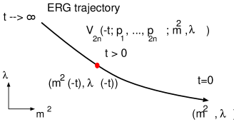
Figure 1: ERG trajectory whose end point at $t=0$ is specified by $(m^{2},\lambda)$

Eq. (69) especially implies that

$$\mathcal{V}_{2n}(-t;p_{1},\cdots,p_{2n};m^{2},\lambda)=\mathcal{V}_{2n}(0;p_{1},\cdots,p_{2n};m^{2}(-t),\lambda(-t))$$ (70)

and hence

$$A_{6}(-t;q,-q,0,0,0,0;\lambda) = A_{6}(0;q,-q,0,0,0,0;\lambda(-t))$$ (71)

$$A_{4}(-t;q,-q,p,-p;\lambda) = A_{4}(0;q,-q,p,-p;\lambda(-t))$$ (72)

$$B_{4}(-t;q,-q,0,0;\lambda) = B_{4}(0;q,-q,0,0;\lambda(-t))$$ (73)

Therefore, using Eqs. (52, 53, 54), the above scaling relations imply that the $t$-dependence of the beta function and anomalous dimensions is given by the running coupling constant:

$$\gamma(-t)=\gamma(\lambda(-t)),\quad\beta_{m}(-t)=\beta_{m}(\lambda(-t)),\quad\beta(-t)=\beta(\lambda(-t))$$ (74)

Using the scaling relation (70), let us rewrite the integral equations. For simplicity, we introduce

$$f(p,m^{2},\lambda)\equiv(1-K(p))\left(\gamma(\lambda)+\frac{\beta_{m}(\lambda)}{2}\frac{m^{2}}{p^{2}+m^{2}}\right)$$ (75)

Then, omitting the first argument “$t=0$” of the vertices, we obtain

$$\mathcal{V}_{2n\geq 6}(p_{1},\cdots,p_{2n};m^{2},\lambda)$$

$$= \int_{0}^{\infty}dt\,\Bigg{[}\,\mathrm{e}^{y_{2n}t}\mathcal{V}_{2n}(p_{1}\mathrm{e}^{-t},\cdots,p_{2n}\mathrm{e}^{-t};m^{2}(-t),\lambda(-t))$$

$$\qquad\qquad\qquad\times\left\{-2n\gamma(\lambda(-(t+t^{\prime})))+\sum_{i=1}^{2n}f(p_{i}\mathrm{e}^{-t},m^{2}(-t),\lambda(-t))\right\}$$

$$\>+\sum_{k=0}^{\left[\frac{n-1}{2}\right]}\sum_{\text{partitions}\atop I+J=\{2n\}}\mathrm{e}^{y_{2(k+1)}t}\mathcal{V}_{2(k+1)}(p_{I}\mathrm{e}^{-t};m^{2}(-t),\lambda(-t))$$

$$\qquad\qquad\times\frac{\Delta(p_{I}\mathrm{e}^{-t})}{p_{I}^{2}+m^{2}(-t)\mathrm{e}^{2t}}\times\mathrm{e}^{y_{2(n-k)}t}\mathcal{V}_{2(n-k)}(p_{J}\mathrm{e}^{-t};m^{2}(-t),\lambda(-t))$$

$$\>+\frac{1}{2}\int_{q}\frac{\Delta(q\mathrm{e}^{-t})}{q^{2}+m^{2}(-t)\mathrm{e}^{2t}}\,\mathrm{e}^{y_{2(n+1)}t}\mathcal{V}_{2(n+1)}(q\mathrm{e}^{-t},-q\mathrm{e}^{-t},p_{1}\mathrm{e}^{-t},\cdots,p_{2n}\mathrm{e}^{-t};m^{2}(-t),\lambda(-t))\>\Bigg{]}$$

For the four-point vertex we obtain

$$\mathcal{V}_{4}(p_{1},\cdots,p_{4};m^{2},\lambda)$$ (77)

$$= \int_{0}^{\infty}dt\,\Bigg{[}\>\mathcal{V}_{4}(p_{1}\mathrm{e}^{-t},\cdots,p_{4}\mathrm{e}^{-t};m^{2}(-t),\lambda(-t))$$

$$\qquad\qquad\qquad\times\left\{-4\gamma(\lambda(-t))+\sum_{i=1}^{4}f(p_{i}\mathrm{e}^{-t},m^{2}(-t),\lambda(-t))\right\}$$

$$\>+\frac{1}{2}\int_{q}\frac{\Delta(q\mathrm{e}^{-t})}{q^{2}+m^{2}(-t)\mathrm{e}^{2t}}\,\mathrm{e}^{-2t}\mathcal{V}_{6}(q\mathrm{e}^{-t},-q\mathrm{e}^{-t},p_{1}\mathrm{e}^{-t},\cdots,p_{4}\mathrm{e}^{-t};m^{2}(-t),\lambda(-t))$$

$$\>+\sum_{i=1}^{4}\mathrm{e}^{2t}\mathcal{V}_{2}(p_{i}\mathrm{e}^{-t};m^{2}(-t),\lambda(-t))\frac{\Delta(p_{i}\mathrm{e}^{-t})}{p_{i}^{2}+m^{2}(-t)\mathrm{e}^{2t}}\mathcal{V}_{4}(p_{1}\mathrm{e}^{-t},\cdots,p_{4}\mathrm{e}^{-t};m^{2}(-t),\lambda(-t))$$

$$\qquad\qquad+\quad\beta(\lambda(-t))\quad\Bigg{]}-\lambda$$

Finally, for the two-point vertex we obtain

$$\mathcal{V}_{2}(p;m^{2},\lambda)$$ (78)

$$= \int_{0}^{\infty}dt\,\Bigg{[}\,-2\gamma(\lambda(-t))\,\mathrm{e}^{2t}\left\{\mathcal{V}_{2}(p\mathrm{e}^{-t};m^{2}(-t),\lambda(-t))-a_{2}(\lambda(-t))\right\}$$

$$\quad+2f(p\mathrm{e}^{-t},m^{2}(-t),\lambda(-t))\,\mathrm{e}^{2t}\mathcal{V}_{2}(p\mathrm{e}^{-t};m^{2}(-t),\lambda(-t))$$

$$+2\gamma(\lambda(-t))\cdot(p^{2}+m^{2}(-t)\mathrm{e}^{2t})+\beta_{m}(\lambda(-t))\cdot m^{2}(-t)\mathrm{e}^{2t}$$

$$+\frac{1}{2}\int_{q}\Bigg{\{}\frac{\Delta(q\mathrm{e}^{-t})}{q^{2}+m^{2}(-t)\mathrm{e}^{2t}}\mathcal{V}_{4}(q\mathrm{e}^{-t},-q\mathrm{e}^{-t},p\mathrm{e}^{-t},-p\mathrm{e}^{-t};m^{2}(-t),\lambda(-t))$$

$$\qquad\qquad-\frac{\Delta(q\mathrm{e}^{-t})}{q^{2}}A_{4}(q\mathrm{e}^{-t},-q\mathrm{e}^{-t},0,0;\lambda(-t))\Bigg{\}}$$

$$+\left(\mathrm{e}^{2t}\mathcal{V}_{2}(p\mathrm{e}^{-t};m^{2}(-t),\lambda(-t))\right)^{2}\frac{\Delta(p\mathrm{e}^{-t})}{p^{2}+m^{2}(-t)\mathrm{e}^{2t}}\>\Bigg{]}+a_{2}(\lambda)$$

In the above $\lambda(-t)$ is defined by

$$-\lambda(-t)\equiv A_{4}(0,0,0,0;\lambda(-t)),$$ (79)

and it gives the solution of

$$-\frac{d}{dt}\lambda(-t)=\beta(\lambda(-t))$$ (80)

satisfying the initial condition $\lambda(0)=\lambda$. The running squared mass is given by

$$m^{2}(-t)\mathrm{e}^{2t}=m^{2}\exp\left[-\int_{0}^{t}dt^{\prime}\beta_{m}(\lambda(-t^{\prime}))\right]$$ (81)

In the integral equation for $\mathcal{V}_{2}$, we have introduced a new notation

$$a_{2}(\lambda)\equiv A_{2}(0,0;\lambda)$$ (82)

Using the scaling relation, the differential equation (V) gives

$$2a_{2}(\lambda)=\beta(\lambda)a_{2}^{\prime}(\lambda)+2\gamma(\lambda)a_{2}(\lambda)-\frac{1}{2}\int_{q}\frac{\Delta(q)}{q^{2}}A_{4}(q,-q,0,0;\lambda)$$ (83)

which has a unique solution if $a_{2}(\lambda)$ is obtained as a power series in $\lambda$.

The integral equations (V, 77, 78) and the equations (79, 81), and (83) constitute the main results of this section. To collect all the main results in a single place, we also repeat the definitions (52, 53, 54) of the beta function and anomalous dimensions, this time using the scaling relation:

$$2\gamma(\lambda) \equiv -\frac{1}{2}\frac{\partial}{\partial p^{2}}\left(\int_{q}\frac{\Delta(q)}{q^{2}}\,A_{4}(q,-q,p,-p;\lambda)\right)_{p^{2}=0}$$ (84)

$$\beta_{m}(\lambda)+2\gamma(\lambda) \equiv \frac{1}{2}\int_{q}\Delta(q)\left(\frac{A_{4}(q,-q,0,0;\lambda)}{q^{4}}-\frac{B_{4}(q,-q,0,0;\lambda)}{q^{2}}\right)$$ (85)

$$\beta(\lambda)+4\lambda\cdot\gamma(\lambda) \equiv -\frac{1}{2}\int_{q}\frac{\Delta(q)}{q^{2}}\,A_{6}(q,-q,0,0,0,0;\lambda)$$ (86)

Our integral equations determine the continuum limit directly. Solved recursively, the integral equations give the interaction vertices as power series in $\lambda$. For a general algorithm, please refer to sect. IV of Ref. Sonoda, . The advantage of the integral equations given above over those obtained in Ref. Sonoda, is twofold:

1. there are only two free parameters instead of four

2. the scaling relation (70) is valid for the vertices

The second point is especially meaningful: the entire scale dependence of the interaction vertices reduces to that of the running parameters. For the above two points, it was crucial that we have modified the ERG transformation so that the conditions

$$\frac{\partial}{\partial p^{2}}A_{2}(p;\lambda)\Big{|}_{p^{2}=0}=B_{2}(p=0;\lambda)=0$$ (87)

are preserved.

The beta function $\beta$ and the anomalous dimensions $\beta_{m},\gamma$ depend on the choice of the momentum cutoff function $K(p)$. We will discuss the dependence in the next section. In Appendix A we compute $\beta$, $\beta_{m}$, $\gamma$ up to two-loop for the choice $K(p)=\theta(1-p^{2})$, and show that the non-universal part (the order $\lambda^{2}$ term of $\beta_{m}$) agrees with the result of the minimal subtraction scheme in dimensional regularization.

VI More general counterterms

To prepare for the discussion of universality in sect. VII we need to generalize the construction of counterterms in sect. III.

Our starting point is the modified action $S^{\prime}[\phi]$ given by Eq. (26). We introduce a further change of variables:

$$\phi(p)\longrightarrow\phi(p)\left(1+\frac{1}{2}(K(p)t(p)+u(p))\right)$$ (88)

where we impose

$$t(p)=u(p)=0\quad\text{for}\quad p^{2}<1$$ (89)

This changes the action $S^{\prime}[\phi]$ to the following:

$$\tilde{S}[\phi] = \frac{1}{2}\int_{p}\phi(p)\phi(-p)\,\frac{p^{2}+m^{2}+\epsilon m^{2}}{K(p)}\left(1+K(p)t(p)+u(p)\right)$$ (90)

$$-\sum_{n=1}^{\infty}\frac{1}{(2n)!}\int_{p_{1},\cdots,p_{2n-1}}\phi(p_{1})\cdots\phi(p_{2n})$$

$$\qquad\qquad\times\mathcal{V}^{\prime}_{2n}(p_{1},\cdots,p_{2n})\left(1+\frac{1}{2}\sum_{i=1}^{2n}(K(p_{i})t(p_{i})+u(p_{i}))\right)$$

where the primed vertices $\mathcal{V}^{\prime}_{2n}$ and $s(p)$ are given by Eqs. (27, 28) and (24), respectively.

The coefficient of the quadratic term can be calculated as follows:

$$\left(\frac{p^{2}+m^{2}+\epsilon m^{2}}{K(p)}-\mathcal{V}^{\prime}_{2}(p)\right)\left(1+K(p)t(p)+u(p)\right)=\frac{p^{2}+m^{2}+\epsilon m^{2}}{K(p)}(1+u(p))$$

$$\qquad\qquad\qquad+t(p)(p^{2}+m^{2})-V^{\prime}_{2}(p)(1+K(p)t(p)+u(p))$$ (91)

We treat the second line of the right-hand side as a vertex, and define the propagator using only the first line. The propagator is then given by

$$\frac{K(p)}{p^{2}+m^{2}+\epsilon m^{2}}-\frac{K(p)u(p)}{p^{2}+m^{2}}$$ (92)

The condition (89) implies that the second term of the propagator is non-vanishing only for $1<p^{2}<2^{2}$.

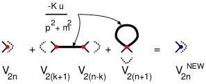
Figure 2: Reinterpretation of Feynman graphs gives new vertices.

In a Feynman diagram with the above propagator, we can interpret the second term not as part of a propagator but as part of an interaction vertex. This reinterpretation is familiar from the derivation of the exact renormalization group equation.Polchinski (1984) (See FIG. 2.) With this reinterpretation, the action $\tilde{S}[\phi]$ is transformed into

$$S^{\prime\prime}[\phi] = \int_{p}\frac{1}{2}\frac{p^{2}+m^{2}+\epsilon m^{2}}{K(p)}\,\phi(p)\phi(-p)$$ (93)

$$\quad-\sum_{n=1}^{\infty}\frac{1}{(2n)!}\int_{p_{1},\cdots,p_{2n-1}}\phi(p_{1})\cdots\phi(p_{2n})\,\mathcal{V}^{\prime\prime}_{2n}(p_{1},\cdots,p_{2n})$$

where

$$\mathcal{V}^{\prime\prime}_{2}(p) = \epsilon m^{2}+\eta(p^{2}+m^{2})-t(p)(p^{2}+m^{2})+\mathcal{V}_{2}(p)(1+\tilde{s}(p))$$ (94)

$$-\mathcal{V}_{2}(p)\frac{K(p)u(p)}{p^{2}+m^{2}}\mathcal{V}_{2}(p)-\frac{1}{2}\int_{q}\frac{K(q)u(q)}{q^{2}+m^{2}}\,\mathcal{V}_{4}(q,-q,p,-p)$$

$$\mathcal{V}^{\prime\prime}_{2n}(p_{1},\cdots,p_{2n}) = \mathcal{V}_{2n}(p_{1},\cdots,p_{2n})\left(1+\frac{1}{2}\sum_{i=1}^{2n}\tilde{s}(p_{i})\right)$$ (95)

$$-\sum_{k=0}^{\left[\frac{n-1}{2}\right]}\sum_{\text{partitions}\atop I+J=\{2n\}}\mathcal{V}_{2(k+1)}(p_{I})\frac{K\left(p_{I}\right)u\left(p_{I}\right)}{p_{I}^{2}+m^{2}}\mathcal{V}_{2(n-k)}(p_{J})$$

$$-\frac{1}{2}\int_{q}\frac{K(q)u(q)}{q^{2}+m^{2}}\,\mathcal{V}_{2(n+1)}(q,-q,p_{1},\cdots,p_{2n})$$

and

$$\tilde{s}(p)\equiv-\eta+(1-K(p))\left(\frac{\epsilon m^{2}}{p^{2}+m^{2}}+\eta\right)+K(p)t(p)+u(p)$$ (96)

By construction the actions $S[\phi]$, given by (20), and $S^{\prime\prime}[\phi]$ are equivalent, since they are merely related by an infinitesimal change of field variables

$$\phi(p)\longrightarrow\phi(p)\left(1+\frac{1}{2}\tilde{s}(p)\right)$$ (97)

From

$$\tilde{s}(p)=-\eta\quad\text{for}\quad p^{2}<1$$ (98)

we obtain

$$\left\langle~{}\phi(p_{1})\cdots\phi(p_{2n-1})\phi~{}\right\rangle_{m^{2};\mathcal{V}}=\left(1-n\eta\right)\left\langle~{}\phi(p_{1})\cdots\phi(p_{2n-1})\phi~{}\right\rangle_{m^{2}+\epsilon m^{2};\mathcal{V}^{\prime\prime}}$$ (99)

if $(\forall i)p_{i}^{2}<1$.

Using only a linear change of field variables, the above counterterms are as general as one can get, and this is just what we need in the next section. We will use the equivalence of $S[\phi]$ and $S^{\prime\prime}[\phi]$ in the discussion of universality.

VII Universality

Universality has been discussed in sect. V of Ref. Sonoda, in the context of the original ERG equation. The purpose of this section is to provide a fuller discussion of universality for the modified ERG equation, and thereby we wish to complete the arguments partially presented in Ref. Sonoda, .

The idea of universality has a broad meaning, but in this section we restrict ourselves to the question of how the vertices in the continuum limit depend on the choice of the momentum cutoff function $K(p)$. Given a choice of $K(p)$, all the interaction vertices $\{V_{2n}\}$ are determined uniquely by a squared mass $m^{2}$ and self-coupling constant $\lambda$, as we have seen in the previous section. When we change $K(p)$, the interaction vertices change even with the same choice of $m^{2}$ and $\lambda$, and the Green functions change accordingly. In this section we wish to show that an arbitrary infinitesimal change of $K(p)$ can be compensated by the corresponding infinitesimal changes in $m^{2}$, $\lambda$, and normalization of the field, and we wish to derive explicit formulas for the changes.

In sect. V we have concluded that the interaction vertices are uniquely specified by a squared mass $m^{2}$, a self-coupling constant $\lambda$, and a choice of the momentum cutoff function $K(p)$. To express the dependence explicitly, let us denote the interaction vertices by $\{\mathcal{V}^{K}_{2n}(p_{1},\cdots,p_{2n};m^{2},\lambda)\}$. We also denote the Green functions calculated with the propagator

$$\frac{K(p)}{p^{2}+m^{2}}$$ (100)

and the vertices $\{\mathcal{V}^{K}_{2n}(p_{1},\cdots,p_{2n};m^{2},\lambda)\}$ by

$$\left\langle~{}\phi(p_{1})\cdots\phi(p_{2n-1})\phi~{}\right\rangle^{K}_{m^{2},\lambda}$$ (101)

Using this notation, we can state what we wish to show in this section more clearly. We wish to show the existence of an infinitesimal change $\epsilon(\lambda)m^{2}$ in the squared mass, $\delta\lambda(\lambda)$ in the self-coupling, and $\eta(\lambda)$ in the normalization of the scalar field so that

$$(1-n\eta(\lambda))\left\langle~{}\phi(p_{1})\cdots\phi(p_{2n-1})\phi~{}\right\rangle^{K+\delta K}_{m^{2}(1+\epsilon),\lambda+\delta\lambda}=\left\langle~{}\phi(p_{1})\cdots\phi(p_{2n-1})\phi~{}\right\rangle^{K}_{m^{2},\lambda}$$ (102)

where $\delta K(p)$ is an arbitrary infinitesimal change in the momentum cutoff function satisfying

$$\delta K(p)=0\quad\text{unless}\quad 1<p^{2}<2^{2}$$ (103)

We first observe that the left-hand side of Eq. (102) can be calculated using the propagator

$$\frac{K(p)}{p^{2}+m^{2}(1+\epsilon)}$$ (104)

and the following vertices:

$$\overline{\mathcal{V}}_{2n}(p_{1},\cdots,p_{2n};m^{2}(1+\epsilon),\lambda+\delta\lambda)\equiv\mathcal{V}_{2n}^{K+\delta K}(p_{1},\cdots,p_{2n};m^{2}(1+\epsilon),\lambda+\delta\lambda)$$

$$\quad+\sum_{k=0}^{\left[\frac{n-1}{2}\right]}\sum_{\text{partitions}\atop I+J=\{2n\}}\mathcal{V}_{2(k+1)}^{K}(p_{I};m^{2},\lambda)\frac{\delta K(p_{I})}{p_{I}^{2}+m^{2}}\mathcal{V}_{2(n-k)}^{K}(p_{J};m^{2},\lambda)$$

$$\quad+\frac{1}{2}\int_{q}\frac{\delta K(q)}{q^{2}+m^{2}}\,\mathcal{V}_{2(n+1)}^{K}(q,-q,p_{1},\cdots,p_{2n};m^{2},\lambda)$$ (105)

This results from the same reasoning as given in the previous section: we reinterpret $\delta K$ not as part of a propagator but as part of an interaction vertex. Now, the equivalence (102) can be reexpressed as

$$(1-n\eta(\lambda))\left\langle~{}\phi(p_{1})\cdots\phi(p_{2n-1})\phi~{}\right\rangle_{m^{2}(1+\epsilon);\overline{\mathcal{V}}}=\left\langle~{}\phi(p_{1})\cdots\phi(p_{2n-1})\phi~{}\right\rangle_{m^{2};\mathcal{V}}$$ (106)

where we use the same momentum cutoff function $K(p)$ for both sides.

To go further, we need the results obtained in the previous section. Using Eq. (99), we can rewrite the right-hand side of Eq. (106) to obtain

$$\left\langle~{}\phi(p_{1})\cdots\phi(p_{2n-1})\phi~{}\right\rangle_{m^{2}(1+\epsilon);\overline{\mathcal{V}}}=\left\langle~{}\phi(p_{1})\cdots\phi(p_{2n-1})\phi~{}\right\rangle_{m^{2}(1+\epsilon);\mathcal{V}^{\prime\prime}}$$ (107)

where the vertices $\{\mathcal{V}^{\prime\prime}_{2n}\}$s are given by (94, 95) with the same $\epsilon$ as for the left-hand side. This equality is of course valid if the two sets of vertices $\{\overline{\mathcal{V}}_{2n}\}$ and $\{\mathcal{V}^{\prime\prime}_{2n}\}$ are equal.

The original problem was to show the existence of $\delta\lambda(\lambda)$, $\epsilon(\lambda)$, and $\eta(\lambda)$ so that Eq. (102) holds. Now the problem is reduced to showing the existence of $\delta\lambda(\lambda)$, $\epsilon(\lambda)$, $\eta(\lambda)$, and functions $t(p)$, $u(p)$ so that $\{\overline{\mathcal{V}}_{2n}\}$ and $\{\mathcal{V}^{\prime\prime}_{2n}\}$ become equal. In other words, given an arbitrary infinitesimal $\delta K(p)$, we wish to determine $\delta\lambda(\lambda)$, $\epsilon(\lambda)$, $\eta(\lambda)$, $u(p)$, and $t(p)$ so that the following equalities hold:

$$\mathcal{V}^{K+\delta K}_{2}(p;m^{2}(1+\epsilon(\lambda)),\lambda+\delta\lambda(\lambda))$$ (108)

$$= \epsilon(\lambda)m^{2}+\eta(\lambda)(p^{2}+m^{2})-t(p)(p^{2}+m^{2})+\mathcal{V}_{2}(p;m^{2},\lambda)(1+\tilde{s}(p))$$

$$\quad-\mathcal{V}_{2}(p;m^{2},\lambda)\frac{\delta K(p)+K(p)u(p)}{p^{2}+m^{2}}\mathcal{V}_{2}(p;m^{2},\lambda)$$

$$\quad-\frac{1}{2}\int_{q}\frac{\delta K(q)+K(q)u(q)}{q^{2}+m^{2}}\,\mathcal{V}_{4}(q,-q,p,-p;m^{2},\lambda)$$

and

$$\mathcal{V}^{K+\delta K}_{2n\geq 4}(p_{1},\cdots,p_{2n};m^{2}(1+\epsilon(\lambda)),\lambda+\delta\lambda(\lambda))$$ (109)

$$= \mathcal{V}_{2n}(p_{1},\cdots,p_{2n};m^{2},\lambda)\left(1+\frac{1}{2}\sum_{i=1}^{2n}\tilde{s}(p_{i})\right)$$

$$\quad-\sum_{k=0}^{\left[\frac{n-1}{2}\right]}\sum_{\text{partitions}\atop I+J=\{2n\}}\mathcal{V}_{2(k+1)}(p_{I};m^{2},\lambda)\frac{\delta K(p_{I})+K\left(p_{I}\right)u\left(p_{I}\right)}{p_{I}^{2}+m^{2}}\mathcal{V}_{2(n-k)}(p_{J};m^{2},\lambda)$$

$$\quad-\frac{1}{2}\int_{q}\frac{\delta K(q)+K(q)u(q)}{q^{2}+m^{2}}\,\mathcal{V}_{2(n+1)}(q,-q,p_{1},\cdots,p_{2n};m^{2},\lambda)$$

where

$$\tilde{s}(p)\equiv-\eta(\lambda)+(1-K(p))\left(\frac{\epsilon(\lambda)m^{2}}{p^{2}+m^{2}}+\eta(\lambda)\right)+K(p)t(p)+u(p)$$ (110)

Note that we have omitted the superscript $K$ from the vertices on the right-hand sides. The functions $t(p)$, $u(p)$ depend also on $\lambda$ and $m^{2}$, and more appropriate notations would be $t(p;m^{2},\lambda)$ and $u(p;m^{2},\lambda)$.

In the remainder of this section, we will show that with an appropriate choice for the functions $u(p;m^{2},\lambda)$ and $t(p;m^{2},\lambda)$, the right-hand sides of Eqs. (108, 109) satisfy the ERG equations expected of the left-hand sides. Since the vertices are determined completely by the ERG equations, this will prove the equality.

The proof is given in three steps. In the first step, we notice that $\epsilon(\lambda)$, $\eta(\lambda)$, and $\delta\lambda(\lambda)$ are determined by $\delta K(p)$ and $u(p)$ as a consequence of the convention (87) and the definition (79) of $\lambda$. Using the obvious notation, and assuming Eqs. (108, 109) are valid, we find the following:

$$\frac{\partial}{\partial p^{2}}A_{2}^{K+\delta K}(p;\lambda+\delta\lambda)\Big{|}_{p^{2}=0}$$

$$\qquad=\eta-\frac{1}{2}\frac{\partial}{\partial p^{2}}\left(\int_{q}\frac{\delta K(q)+K(q)u(q;0,\lambda)}{q^{2}}\,A_{4}(q,-q,p,-p)\right)_{p^{2}=0}$$ (111)

$$B_{2}^{K+\delta K}(0;\lambda+\delta\lambda)$$

$$\qquad=\epsilon+\eta-\frac{1}{2}\int_{q}(\delta K(q)+K(q)u(q;0,\lambda))\left(-\frac{A_{4}(q,-q,0,0)}{q^{4}}+\frac{B_{4}(q,-q,0,0)}{q^{2}}\right)$$

$$\qquad\qquad-\frac{1}{2}\int_{q}\frac{K(q)\frac{\partial}{\partial m^{2}}u(q;m^{2},\lambda)\Big{|}_{m^{2}=0}}{q^{2}}A_{4}(q,-q,0,0)$$ (112)

$$A_{4}^{K+\delta K}(0,0,0,0;\lambda+\delta\lambda)$$

$$\qquad=(-\lambda)(1-2\eta)-\frac{1}{2}\int_{q}\frac{\delta K(q)+K(q)u(q;0,\lambda)}{q^{2}}\,A_{6}(q,-q,0,0,0,0)$$ (113)

For Eqs. (108, 109) to be valid, these three equations must be satisfied. The first two must vanish, while the last must equal $-(\lambda+\delta\lambda)$. Hence, we must obtain

$$\eta = \frac{1}{2}\frac{\partial}{\partial p^{2}}\left(\int_{q}\frac{\delta K(q)+K(q)u(q;0,\lambda)}{q^{2}}\,A_{4}(q,-q,p,-p)\right)_{p^{2}=0}$$ (114)

$$\epsilon+\eta = \frac{1}{2}\int_{q}(\delta K(q)+K(q)u(q;0,\lambda))\left(-\frac{1}{q^{4}}A_{4}(q,-q,0,0)+\frac{1}{q^{2}}B_{4}(q,-q,0,0)\right)$$ (115)

$$\qquad+\frac{1}{2}\int_{q}\frac{K(q)\frac{\partial}{\partial m^{2}}u(q;m^{2},\lambda)\Big{|}_{m^{2}=0}}{q^{2}}\,A_{4}(q,-q,0,0)$$

$$\delta\lambda+2\lambda\cdot\eta = \frac{1}{2}\int_{q}\frac{\delta K(q)+K(q)u(q;0,\lambda)}{q^{2}}\,A_{6}(q,-q,0,0,0,0)$$ (116)

Thus, $\epsilon$, $\eta$, and $\delta\lambda$ are determined by $\delta K$ and $u$. Therefore, we only need to determine the functions $u(p;m^{2},\lambda)$ and $t(p;m^{2},\lambda)$.

The second step is to determine the changes in the beta function and anomalous dimensions due to the changes of the parameters $m^{2},\lambda$ and normalization of the field. The result is well known. By considering the running of $\lambda+\delta\lambda$, $m^{2}(1+\epsilon)$, and $(1+\eta/2)\phi$, we obtain the following results up to first order in $\delta K$:

$$\beta^{K+\delta K}(\lambda+\delta\lambda)-\beta(\lambda) = \delta\lambda^{\prime}(\lambda)\cdot\beta(\lambda)$$ (117)

$$\beta_{m}^{K+\delta K}(\lambda+\delta\lambda)-\beta_{m}(\lambda) = \epsilon^{\prime}(\lambda)\cdot\beta(\lambda)$$ (118)

$$\gamma^{K+\delta K}(\lambda+\delta\lambda)-\gamma(\lambda) = \frac{1}{2}\eta^{\prime}(\lambda)\cdot\beta(\lambda)$$ (119)

where the primes denote derivatives with respect to $\lambda$. We do not actually need $\beta^{K+\delta K}$ since only $\beta_{m}^{K+\delta K}$ and $\gamma^{K+\delta K}$ enter into the modified ERG differential equations for $\{\mathcal{V}^{K+\delta K}_{2n}\}$.

In the final step we demand that the right-hand sides of (108, 109) satisfy the modified ERG differential equations expected of $\{\mathcal{V}^{K+\delta K}_{2n}(m^{2}(1+\epsilon),\lambda+\delta\lambda)\}$. This step is straightforward, but requires somewhat lengthy calculations. We omit the intermediate results. Remarkably, all boil down to the following equations for $u(p;m^{2},\lambda)$ and $t(p;m^{2},\lambda)$:

$$\frac{d}{dt}u(p) = (\delta K(p)+K(p)u(p))\left(2\gamma+\beta_{m}\frac{m^{2}}{p^{2}+m^{2}}\right)+\Delta(p)\left(\frac{\epsilon m^{2}}{p^{2}+m^{2}}+\eta-t(p)\right)$$ (120)

$$\frac{d}{dt}t(p) = u(p)\left(2\gamma+\beta_{m}\frac{m^{2}}{p^{2}+m^{2}}\right)$$ (121)

where we have defined the RG differential operator acting on functions of $p^{2}$, $m^{2}$, and $\lambda$ as

$$\frac{d}{dt}\equiv 2p^{2}\frac{\partial}{\partial p^{2}}+\beta(\lambda)\frac{\partial}{\partial\lambda}+(2+\beta_{m}(\lambda))m^{2}\frac{\partial}{\partial m^{2}}$$ (122)

The above differential equations can be solved perturbatively in powers of $\lambda$, and thanks to the vanishing condition (89), the solutions for $u(p),t(p)$ are unique. It is easy to see that $u$ is of order $\lambda$, and $t$ is of order $\lambda^{2}$. We will compute $u(p)$ and $t(p)$ to the lowest nontrivial order in $\lambda$ in Appendix C. This concludes the proof of the equality $\overline{\mathcal{V}}=\mathcal{V}^{\prime\prime}$, which proves Eq. (102). Thus, we have established universality of the continuum limit.

Finally, a short comment is in order, regarding sect. V of Ref. Sonoda, . If we demand that $\mathcal{V}^{K+\delta K}$ given by (108, 109) satisfy the original ERG equation with no $\beta,\beta_{m}$, or $\gamma$, we obtain

$$u(p)=(1-K(p))\left(\frac{\epsilon m^{2}}{p^{2}+m^{2}}+\eta\right)$$ (123)

and $t(p)=0$, where $\epsilon,\eta$ are arbitrary infinitesimal constants. This is easily obtained from Eqs. (120, 121) by taking $\beta_{m}$ and $\gamma$ to zero. This result was quoted without proof in sect. V of Ref. Sonoda, . This will be also used in Appendix B.

VIII Concluding remarks

It is easy to summarize what we have done in this paper. We have united Wilson’s exact renormalization group with the standard renormalization group of running parameters in renormalized field theories. We have modified the ERG differential equation in such a way that the continuum limit is parameterized by a squared mass and a self-coupling constant. The scale dependence of the infinite number of interaction vertices is given through the scale dependence of the two running parameters. We have called this a scaling relation, and it is expressed by Eq. (69) or (70).

The integral equation that we have introduced in Ref. Sonoda, and the present paper can be a powerful tool. It is a defining equation of a so-called “perfect action” that describes the continuum limit in terms of a theory with a finite momentum cutoff. It is especially interesting to see how the symmetry of the continuum limit, such as chiral symmetry and gauge symmetry, is realized in a perfect action. We believe that our integral equation will provide a powerful quantitative tool to address this question.

As one of the nice properties of the framework introduced in this paper, we have mentioned the mass independence in sect. I. The mass independence means not only that the squared mass renormalizes multiplicatively, but also that we have a broken phase for $m^{2}<0$. We have discussed the broken phase in Appendix D.

Concerning the issue of universality discussed in sect. VII, we have one technical remark. We know that the beta function and anomalous dimensions depend on the choice of the momentum cutoff function $K(p)$. Now, what choice gives the same $\beta,\beta_{m},\gamma$ as the minimal subtraction scheme in dimensional regularization? We speculate the step function $K(p)=\theta(1-p^{2})$ is the answer, but this is only supported by a single calculation of $\beta_{m}$ at order $\lambda^{2}$ in Appendix A. It will be interesting to know the answer.

In calculating the vertices recursively using the integral equations, we have noticed the great facility brought by expressing the integrand (with respect to $t$) as a total derivative. Following the recursive procedure blindly is a tedious task. It will be extremely interesting and useful to come up with a short-cut procedure to construct the vertices in the continuum limit.

Appendix A Explicit calculations of $\beta$, $\beta_{m}$, and $\gamma$

In this appendix we sketch the calculations of the beta function and anomalous dimensions. The style of presentation is not uniform: some parts are given in more detail than others. As is usual with perturbative calculations, the difficulty is mainly in doing momentum integrals.

We first recall the general formulas for the beta function $\beta(\lambda)$ and anomalous dimensions $\beta_{m}(\lambda)$, $\gamma(\lambda)$:

$$2\gamma(\lambda) \equiv -\frac{\partial}{\partial p^{2}}\left[\frac{1}{2}\int_{q}\frac{\Delta(q)}{q^{2}}\,A_{4}(q,-q,p,-p;\lambda)\right]_{p^{2}=0}$$ (124)

$$2\gamma(\lambda)+\beta_{m}(\lambda) \equiv \frac{1}{2}\int_{q}\left\{\frac{\Delta(q)}{q^{4}}A_{4}(q,-q,0,0;\lambda)-\frac{\Delta(q)}{q^{2}}B_{4}(q,-q,0,0;\lambda)\right\}$$ (125)

$$\beta(\lambda)+4\lambda\cdot\gamma(\lambda) \equiv -\frac{1}{2}\int_{q}\frac{\Delta(q)}{q^{2}}A_{6}(q,-q,0,0,0,0;\lambda)$$ (126)

where $A_{4},B_{4}$, and $A_{6}$ are the coefficients of the vertices expanded in powers of $m^{2}$:

$$\mathcal{V}_{2n}(p_{1},\cdots,p_{2n};m^{2},\lambda)=A_{2n}(p_{1},\cdots,p_{2n};\lambda)+m^{2}B_{2n}(p_{1},\cdots,p_{2n};\lambda)+\text{O}(m^{4})$$ (127)

$\beta$ is universal to order $\lambda^{3}$, $\gamma$ to order $\lambda^{2}$, and $\beta_{m}$ only up to order $\lambda$. The non-universal higher order terms depend on the choice of the momentum cutoff function $K(p)$. In the following we evaluate $\beta_{m},\gamma$ to order $\lambda^{2}$, and $\beta$ to order $\lambda^{3}$. Only the order $\lambda^{2}$ term of $\beta_{m}$ is non-universal. Except for this non-universal term and the third order term of $\beta$, the lowest order terms have been computed in Ref. Hughes and Liu, 1988 by Hughes and Liu. Our results must and do agree with theirs because of the universality.

We will need to calculate $A_{4},B_{4}$ to order $\lambda^{2}$, and $A_{6}$ to order $\lambda^{3}$. We will use the notation such as

$$A_{2}(p;\lambda)=\sum_{i=1}^{\infty}(-\lambda)^{i}A_{2}^{(i)}(p),\quad\mathcal{V}_{2}(p;\lambda,m^{2})=\sum_{i=1}^{\infty}(-\lambda)^{i}\mathcal{V}_{2}^{(i)}(p;m^{2})$$ (128)

to denote the order of expansions in $\lambda$. We refer the reader to section IV of Ref. Sonoda, for a general algorithm for perturbative calculations of the interaction vertices.

A.1 Order $\lambda$

A.1.1 $4$-point

Our starting point is

$$\mathcal{V}_{4}^{(1)}(p_{1},\cdots,p_{4})=1$$ (129)

implying

$$A_{4}^{(1)}(p_{1},\cdots,p_{4})=1,\quad B_{4}^{(1)}(p_{1},\cdots,p_{4})=0$$ (130)

Hence,

$$\gamma^{(1)}=0$$ (131)

and

$$\beta_{m}^{(1)}=\frac{1}{2}\int_{q}\frac{\Delta(q)}{q^{4}}A_{4}^{(1)}=\frac{1}{2}\int_{q}\frac{\Delta(q)}{q^{4}}=\frac{1}{(4\pi)^{2}}$$ (132)

where the integrand is a total derivative due to Eq. (10). Hence, the running squared mass is given by

$$m^{2}(-t)\mathrm{e}^{2t}=m^{2}\left(1-t\cdot(-\lambda)\cdot\beta_{m}^{(1)}+\text{O}(\lambda^{2})\right)$$ (133)

A.1.2 $2$-point

Eq. (83) gives

$$a_{2}^{(1)}=-\frac{1}{4}\int_{q}\frac{\Delta(q)}{q^{2}}A_{4}^{(1)}=-\frac{1}{4}\int_{q}\frac{\Delta(q)}{q^{2}}$$ (134)

This depends on the choice of the cutoff function $K(p)$. We then find

$$\mathcal{V}_{2}^{(1)}(m^{2}) = \int_{0}^{\infty}dt\left[\frac{1}{2}\int_{q}\left\{\frac{\Delta(q\mathrm{e}^{-t})}{q^{2}+m^{2}}-\frac{\Delta(q\mathrm{e}^{-t})}{q^{2}}\right\}+\beta_{m}^{(1)}m^{2}\right]+a_{2}^{(1)}$$ (135)

$$= \frac{m^{4}}{2}\int_{q}\frac{1-K(q)}{q^{4}(q^{2}+m^{2})}+a_{2}^{(1)}$$

Note that the two-point vertex is momentum independent at this order.

A.2 Order $\lambda^{2}$

A.2.1 $6$-point

From

$$\mathcal{V}_{6}^{(2)}(p_{1},\cdots,p_{6};m^{2})=\frac{1-K(p_{1}+p_{2}+p_{3})}{(p_{1}+p_{2}+p_{3})^{2}+m^{2}}+\text{9 permutations}$$ (136)

we obtain

$$A_{6}^{(2)}(q,-q,0,0,0,0)=6\frac{1-K(q)}{q^{2}}$$ (137)

Hence, we get

$$\beta^{(2)}=-\frac{1}{2}\int_{q}\frac{\Delta(q)}{q^{2}}A_{6}^{(2)}(q,-q,0,0,0,0)=-3\int_{q}\frac{\Delta(q)(1-K(q))}{q^{4}}=-\frac{3}{(4\pi)^{2}}$$ (138)

using

$$\Delta(q)(1-K(q))=q^{2}\frac{d}{dq^{2}}(1-K(q))^{2}$$ (139)

Therefore, the running coupling is given by

$$\lambda(-t)=\lambda-t(-\lambda)^{2}\beta^{(2)}+\text{O}(\lambda^{3})$$ (140)

A.2.2 $4$-point

The integral ERG equation (77) gives

$$\mathcal{V}_{4}^{(2)}(p_{1},\cdots,p_{4};m^{2})$$ (141)

$$= \int_{0}^{\infty}dt\,\Bigg{[}\,\sum_{i=1}^{4}\mathrm{e}^{2t}\mathcal{V}_{2}^{(1)}(m^{2}\mathrm{e}^{-2t})\frac{\Delta(p_{i}\mathrm{e}^{-t})}{p_{i}^{2}+m^{2}}+\frac{1}{2}\beta_{m}^{(1)}m^{2}\sum_{i=1}^{4}\frac{1-K(p_{i}\mathrm{e}^{-t})}{p_{i}^{2}+m^{2}}$$

$$\qquad+\frac{1}{2}\int_{q}\frac{\Delta(q\mathrm{e}^{-t})}{q^{2}+m^{2}}\Bigg{\{}\sum_{i=1}^{4}\frac{1-K(p_{i}\mathrm{e}^{-t})}{p_{i}^{2}+m^{2}}$$

$$\qquad\qquad+2\left(\frac{1-K((p_{1}+p_{2}+q)\mathrm{e}^{-t})}{(p_{1}+p_{2}+q)^{2}+m^{2}}+\text{2 permutations}\right)\Bigg{\}}\,+\beta^{(2)}\>\Bigg{]}$$

Using the ERG differential equation

$$-\frac{\partial}{\partial t}\left(\mathrm{e}^{2t}\mathcal{V}_{2}^{(1)}(m^{2}\mathrm{e}^{-2t})\right)=\frac{1}{2}\int_{q}\frac{\Delta(q\mathrm{e}^{-t})}{q^{2}+m^{2}}+m^{2}\beta_{m}^{(1)}$$ (142)

and integration by parts, we obtain

$$\mathcal{V}_{4}^{(2)}(p_{1},\cdots,p_{4};m^{2})=\mathcal{V}_{2}^{(1)}(m^{2})\sum_{i=1}^{4}\frac{1-K(p_{i})}{p_{i}^{2}+m^{2}}-\frac{1}{2}\beta_{m}^{(1)}m^{2}\sum_{i=1}^{4}\frac{\int_{0}^{\infty}dt(1-K(p_{i}\mathrm{e}^{-t}))}{p_{i}^{2}+m^{2}}$$

$$\quad+\int_{0}^{\infty}dt\left[\,\int_{q}\frac{\Delta(q\mathrm{e}^{-t})}{q^{2}+m^{2}}\left(\frac{1-K((p_{1}+p_{2}+q)\mathrm{e}^{-t})}{(p_{1}+p_{2}+q)^{2}+m^{2}}+\text{2 permutations}\right)+\beta^{(2)}\>\right]$$ (143)

Expanding this in powers of $m^{2}$, we obtain

$$A_{4}^{(2)}(p,-p,0,0)=2a_{2}^{(1)}\frac{1-K(p)}{p^{2}}$$

$$\qquad\qquad+2\int_{0}^{\infty}dt\int_{q}\frac{\Delta(q\mathrm{e}^{-t})}{q^{2}}\left(\frac{1-K((p+q)\mathrm{e}^{-t})}{(p+q)^{2}}-\frac{1-K(q\mathrm{e}^{-t})}{q^{2}}\right)$$ (144)

$$B_{4}^{(2)}(p,-p,0,0)=-2a_{2}^{(1)}\frac{1-K(p)}{p^{4}}-\beta_{m}^{(1)}\frac{\int_{0}^{\infty}dt(1-K(p\mathrm{e}^{-t}))}{p^{2}}$$

$$\qquad\qquad-2\int_{q}\frac{1-K(q)}{q^{4}}\frac{1-K(p+q)}{(p+q)^{2}}-\int_{q}\frac{\Delta(q)(1-K(q))}{q^{6}}$$ (145)

and for $p^{\prime 2}<1$ we obtain

$$A_{4}^{(2)}(p^{\prime},-p^{\prime},p,-p)=2a_{2}^{(1)}\frac{1-K(p)}{p^{2}}$$

$$+\int_{0}^{\infty}dt\,\Bigg{[}\,\int_{q}\frac{\Delta(q\mathrm{e}^{-t})}{q^{2}}\left(\frac{1-K((p+p^{\prime}+q)\mathrm{e}^{-t})}{(p+p^{\prime}+q)^{2}}+\frac{1-K((p-p^{\prime}+q)\mathrm{e}^{-t})}{(p-p^{\prime}+q)^{2}}\right)$$

$$\qquad\qquad-2\int_{q}\frac{\Delta(q)(1-K(q))}{q^{4}}\,\Bigg{]}$$ (146)

We first compute

$$-2\gamma^{(2)} = \frac{1}{2}\frac{\partial}{\partial p^{\prime 2}}\int_{p}\frac{\Delta(p)}{p^{2}}A_{4}^{(2)}(p^{\prime},-p^{\prime},p,-p)\Bigg{|}_{p^{\prime 2}=0}$$ (147)

$$= \int_{p}\frac{\Delta(p)}{p^{2}}\int_{0}^{\infty}dt\int_{q}\frac{\Delta(q\mathrm{e}^{-t})}{q^{2}}\frac{\partial}{\partial p^{\prime 2}}\frac{1-K((p+q+p^{\prime})\mathrm{e}^{-t})}{(p+q+p^{\prime})^{2}}\Bigg{|}_{p^{\prime 2}=0}$$

$$= -\frac{1}{2}\int_{0}^{\infty}dt\int_{p}\frac{\Delta(p\mathrm{e}^{t})}{p^{2}}\int_{q}\frac{\Delta(q)}{q^{2}}K^{\prime\prime}(p+q)$$

$$= \int_{p,q}\frac{K(p)}{p^{2}}K^{\prime}(q)K^{\prime\prime}(p+q)$$

where we used

$$\Delta(p\mathrm{e}^{t})=-\partial_{t}K(p\mathrm{e}^{t})\,,$$ (148)

and the primed quantities are defined by

$$K^{\prime}(p)\equiv\frac{d}{dp^{2}}K(p),\quad K^{\prime\prime}(p)\equiv\frac{d^{2}}{(dp^{2})^{2}}K(p)$$ (149)

The last expression in Eq. (147) was calculated by Hughes and Liu Hughes and Liu (1988) as

$$-2\gamma^{(2)}=-\frac{1}{6}\frac{1}{(4\pi)^{2}}$$ (150)

We next compute

$$\beta_{m}^{(2)}+2\gamma^{(2)} = \frac{1}{2}\int_{p}\left\{\frac{\Delta(p)}{p^{4}}A_{4}^{(2)}(p,-p,0,0)-\frac{\Delta(p)}{p^{2}}B_{4}^{(2)}(p,-p,0,0)\right\}$$ (151)

$$= \frac{1}{4}\int_{q}\frac{\Delta(q)}{q^{4}}\int_{p}\frac{(1-K(p))K(p)}{p^{4}}$$

$$+\int_{p}\frac{K(p)}{p^{4}}\int_{q}\frac{1-K(q)}{q^{2}}\left\{\frac{\Delta(p+q)}{(p+q)^{2}}-\frac{\Delta(q)}{q^{2}}\right\}$$

$$+\int_{p}\frac{K(p)}{p^{2}}\int_{q}\left\{\frac{1-K(q)}{q^{2}}\frac{\Delta(p+q)}{(p+q)^{4}}+\frac{1-K(q)}{q^{4}}\frac{\Delta(p+q)}{(p+q)^{2}}\right\}$$

where we have used Eq. (148) to perform several integrals over $t$.

$\beta_{m}^{(2)}$ depends on the choice of the momentum cutoff function $K$. In order to get a concrete value, let us choose the step function

$$K(p)\equiv\theta(1-p^{2})=\left\{\begin{array}[]{r@{\quad\text{if}\quad}l}1&p^{2}<1\\ 0&p^{2}>1\end{array}\right.$$ (152)

The first integral on the right-hand side of (151) vanishes with this choice. For the two remaining double integrals, the integrals over $q$ can be done analytically, but the integrals over $p$ have been done only numerically. The final result is

$$\beta_{m}^{(2)}+2\gamma^{(2)}=\frac{1}{(4\pi)^{4}}$$ (153)

Hence, using Eq. (150), we get

$$\beta_{m}^{(2)}=\frac{1}{(4\pi)^{4}}\frac{5}{6}$$ (154)

This is the same result as in the minimal subtraction (MS) scheme in dimensional regularization. It is interesting to see whether the equivalence of the choice (152) to the MS scheme extends beyond this order.

A.3 Order $\lambda^{3}$

We start from

$$\mathcal{V}_{8}^{(3)}(p_{1},\cdots,p_{8};m^{2})=\frac{1-K(p_{1}+p_{2}+p_{3})}{(p_{1}+p_{2}+p_{3})^{2}+m^{2}}\cdot\frac{1-K(p_{4}+p_{5}+p_{6})}{(p_{4}+p_{5}+p_{6})^{2}+m^{2}}+\text{279 permutations}$$ (155)

By a straightforward enumeration of diagrams, we obtain

$$A_{8}^{(3)}(q,-q,q^{\prime},-q^{\prime},0,0,0,0)=18\left\{\left(\frac{1-K(q)}{q^{2}}\right)^{2}+\left(\frac{1-K(q^{\prime})}{q^{\prime 2}}\right)^{2}\right\}$$

$$+24\left(\frac{1-K(q)}{q^{2}}+\frac{1-K(q^{\prime})}{q^{\prime 2}}\right)\left(\frac{1-K(q+q^{\prime})}{(q+q^{\prime})^{2}}+\frac{1-K(q-q^{\prime})}{(q-q^{\prime})^{2}}\right)$$

$$+24\frac{1-K(q)}{q^{2}}\frac{1-K(q^{\prime})}{q^{\prime 2}}+12\left(\frac{1-K(q+q^{\prime})}{(q+q^{\prime})^{2}}\right)^{2}+12\left(\frac{1-K(q-q^{\prime})}{(q-q^{\prime})^{2}}\right)^{2}$$ (156)

Substituting this into the integral equation for $A_{6}^{(3)}(p,-p,0,0,0,0)$, we eventually obtain

$$A_{6}^{(3)}(p,-p,0,0,0,0)=12\Bigg{[}\,\int_{q}\frac{1-K(q)}{q^{2}}\left(\frac{1-K(p+q)}{(p+q)^{2}}\right)^{2}$$

$$\quad+\frac{1-K(p)}{p^{2}}\int_{q}\frac{1-K(q)}{q^{2}}\left(\frac{1-K(p+q)}{(p+q)^{2}}-\frac{1-K(q^{\prime})}{q^{\prime 2}}\right)\,\Bigg{]}$$ (157)

In getting this result, the integral over the logarithmic scale parameter $t$ has been done by rewriting the integrand as much as possible as a total derivative with respect to $t$.

Therefore, we obtain

$$\beta^{(3)}-4\gamma^{(2)}=-\frac{1}{2}\int_{p}\frac{\Delta(p)}{p^{2}}\,A_{6}^{(3)}(p,-p,0,0,0,0)$$

$$=-6\Bigg{[}\,\int_{p}\frac{\Delta(p)}{p^{2}}\int_{q}\frac{1-K(q)}{q^{2}}\left(\frac{1-K(p+q)}{(p+q)^{2}}\right)^{2}$$ (158)

$$\,+\int_{p}\frac{\Delta(p)(1-K(p))}{p^{4}}\int_{q}\frac{1-K(q)}{q^{2}}\left(\frac{1-K(p+q)}{(p+q)^{2}}-\frac{1-K(q)}{q^{2}}\right)\,\Bigg{]}$$ (159)

This should not depend on the choice of $K$, and we are free to choose $K$ as the step function (152). As before, the integrals over $q$ can be done analytically, but the integrals over $p$ have been done only numerically. Our final result is

$$\beta^{(3)}-4\gamma^{(2)}=-\frac{6}{(4\pi)^{4}}$$ (160)

Hence, using Eq. (150), we obtain

$$\beta^{(3)}=-\frac{17}{3}\frac{1}{(4\pi)^{4}}$$ (161)

This agrees with the standard universal result.

Appendix B Alternative definition of the beta function and anomalous dimensions

In Ref. Hughes and Liu, 1988 Hughes and Liu define a beta function and anomalous dimensions for the $\phi^{4}$ theory. Their definition is unsatisfactory in two respects:

1. It is based upon a careless treatment of counterterms. (See the first paragraph in sect. III.)

2. The renormalization scheme adopted is not mass independent.

In this appendix, we will improve their definition to come up with a mass independent scheme with an alternative beta function and anomalous dimensions. We will treat counterterms carefully using the results of sects. III, VI.

As has been explained in Ref. Sonoda, , in the continuum limit the solution $\{\mathcal{V}_{2n}(t)\}$ of the original ERG equation is parametrized by four parameters: a squared mass $m^{2}$ and three constants of integration $B_{2}(t=0),C_{2}(0),A_{4}(0)$. It is convenient to choose the minimal subtraction scheme:

$$B_{2}(0)=C_{2}(0)=0$$ (162)

so that the vertices $\{\mathcal{V}_{2n}(t)\}$ are determined by $m^{2}$ and $A_{4}(0)$.

As explained in sect. IV, the problem with the above scheme is that (162) is not preserved along the ERG flow. After renormalization by an infinitesimal logarithmic scale $\Delta t$, we have found (see Eqs. (36, 37))

$$B_{2}(\Delta t) = \Delta t\,\frac{1}{2}\int_{q}\Delta(q)\left(\frac{B_{4}(q,-q,0,0)}{q^{2}}-\frac{A_{4}(q,-q,0,0)}{q^{4}}\right)$$ (163)

$$C_{2}(\Delta t) = \Delta t\,\frac{1}{2}\frac{\partial}{\partial p^{2}}\int_{q}\frac{\Delta(q)}{q^{2}}\,A_{4}(q,-q,p,-p)\Bigg{|}_{p^{2}=0}$$ (164)

and (162) is not satisfied anymore.

We will not modify the ERG flow. Instead we proceed by generating a new ERG trajectory $\{\mathcal{V}^{\prime}_{2n}(t)\}$ equivalent to the original trajectory $\{\mathcal{V}_{2n}(t)\}$ in such a way that the convention (162) is satisfied at $t=\Delta t$. This can be done by using the results of sect. VI (see the remark in the last paragraph). We generate $\{\mathcal{V}^{\prime}_{2n}(t)\}$ by introducing generalized counterterms corresponding to the choice

$$u(p)=(1-K(p))\left(\frac{\epsilon m^{2}\mathrm{e}^{2t}}{p^{2}+m^{2}\mathrm{e}^{2t}}+\eta\right),\quad t(p)=0$$ (165)

where $\epsilon,\eta$ are infinitesimal constants independent of $t$. Then, we obtain

$$\mathcal{V}^{\prime}_{2}(t;p)=\epsilon m^{2}\mathrm{e}^{2t}+\eta(p^{2}+m^{2}\mathrm{e}^{2t})$$

$$\quad+\left(1-\eta+2(1-K(p))\left(\frac{\epsilon m^{2}\mathrm{e}^{2t}}{p^{2}+m^{2}\mathrm{e}^{2t}}+\eta\right)\right)\mathcal{V}_{2}(t;p)$$

$$\quad-\mathcal{V}_{2}(t;p)^{2}\frac{K(p)(1-K(p))}{p^{2}+m^{2}\mathrm{e}^{2t}}\left(\frac{\epsilon m^{2}\mathrm{e}^{2t}}{p^{2}+m^{2}\mathrm{e}^{2t}}+\eta\right)$$

$$\quad-\frac{1}{2}\int_{q}\frac{K(q)(1-K(q))}{q^{2}+m^{2}\mathrm{e}^{2t}}\left(\frac{\epsilon m^{2}\mathrm{e}^{2t}}{q^{2}+m^{2}\mathrm{e}^{2t}}+\eta\right)\,\mathcal{V}_{4}(t;q,-q,p,-p)$$ (166)

$$\mathcal{V}^{\prime}_{2n\geq 4}(t;p_{1},\cdots,p_{2n})$$

$$\,=\mathcal{V}_{2n}(t;p_{1},\cdots,p_{2n})\left(1-n\eta+\sum_{i=1}^{2n}(1-K(p_{i}))\left(\frac{\epsilon m^{2}\mathrm{e}^{2t}}{p_{i}^{2}+m^{2}\mathrm{e}^{2t}}+\eta\right)\right)$$

$$\quad-\sum_{k=0}^{\left[\frac{n-1}{2}\right]}\sum_{\text{partitions}\atop I+J=\{2n\}}\mathcal{V}_{2(k+1)}(t;p_{I})\frac{K(p_{I})(1-K(p_{I}))}{p_{I}^{2}+m^{2}\mathrm{e}^{2t}}\left(\frac{\epsilon m^{2}\mathrm{e}^{2t}}{p_{I}^{2}+m^{2}\mathrm{e}^{2t}}+\eta\right)\mathcal{V}_{2(n-k)}(t;p_{J})$$

$$\quad-\frac{1}{2}\int_{q}\frac{K(q)(1-K(q))}{q^{2}+m^{2}\mathrm{e}^{2t}}\left(\frac{\epsilon m^{2}\mathrm{e}^{2t}}{q^{2}+m^{2}\mathrm{e}^{2t}}+\eta\right)\mathcal{V}_{2(n+1)}(t;q,-q,p_{1},\cdots,p_{2n})$$ (167)

The new vertices $\{\mathcal{V}^{\prime}_{2n}(t)\}$ satisfy the original ERG equation, and they are equivalent to $\{\mathcal{V}_{2n}(t)\}$, i.e., they give rise to the same Green functions:

$$\left\langle~{}\phi(p_{1})\cdots\phi(p_{2n-1})\phi~{}\right\rangle_{m^{2}\mathrm{e}^{2t},\mathcal{V}(t)}=(1-n\eta)\left\langle~{}\phi(p_{1})\cdots\phi(p_{2n-1})\phi~{}\right\rangle_{m^{2}(1+\epsilon)\mathrm{e}^{2t},\mathcal{V}^{\prime}(t)}$$ (168)

Eq. (166) gives

$$B^{\prime}_{2}(0) = \epsilon+\eta-\frac{\epsilon}{2}\int_{q}\frac{K(q)(1-K(q))}{q^{4}}A_{4}(q,-q,0,0)$$ (169)

$$\quad-\frac{\eta}{2}\int_{q}K(q)(1-K(q))\left(\frac{B_{4}(q,-q,0,0)}{q^{2}}-\frac{A_{4}(q,-q,0,0)}{q^{4}}\right)$$

$$C^{\prime}_{2}(0) = \eta-\frac{\eta}{2}\frac{\partial}{\partial p^{2}}\left(\int_{q}\frac{K(q)(1-K(q))}{q^{2}}A_{4}(q,-q,p,-p)\right)\Bigg{|}_{p^{2}=0}$$ (170)

Taking $\epsilon,\eta$ of order $\Delta t$, we obtain

$$B^{\prime}_{2}(\Delta t) = B_{2}(\Delta t)+B^{\prime}_{2}(0)$$ (171)

$$C^{\prime}_{2}(\Delta t) = C_{2}(\Delta t)+C^{\prime}_{2}(0)$$ (172)

to first order in $\Delta t$. We can choose the constants $\epsilon,\eta$ so that $\{\mathcal{V}^{\prime}_{2n}(\Delta t)\}$ satisfy the convention (162):

$$B^{\prime}_{2}(\Delta t)=C^{\prime}_{2}(\Delta t)=0$$ (173)

We now have two ERG trajectories: $\{\mathcal{V}_{2n}(t)\}$ and $\{\mathcal{V}^{\prime}_{2n}(t)\}$. They are physically equivalent. The end point $t=0$ of the first trajectory and the end point $t=\Delta t$ of the second satisfy the convention (162). The former end point is specified by $m^{2}$ and $\lambda$, and the latter by $m^{2}\mathrm{e}^{2\Delta t+\epsilon}$ and $-A^{\prime}_{4}(\Delta t)$. If we introduce an alternative beta function and anomalous dimension of the squared mass by

$$\tilde{\beta}(\lambda)\equiv\frac{-A^{\prime}_{4}(\Delta t)+A_{4}(0)}{\Delta t}\,,\quad\tilde{\beta}_{m}(\lambda)\equiv\frac{\epsilon}{\Delta t}\,,$$ (174)

we can specify the end point $t=\Delta t$ of the trajectory $\{\mathcal{V}^{\prime}_{2n}(t)\}$ by

$$m^{2}(\Delta t)\equiv m^{2}\left(1+\Delta t(2+\tilde{\beta}_{m}(\lambda)\right),\quad\lambda(\Delta t)\equiv\lambda+\Delta t~{}\tilde{\beta}(\lambda)$$ (175)

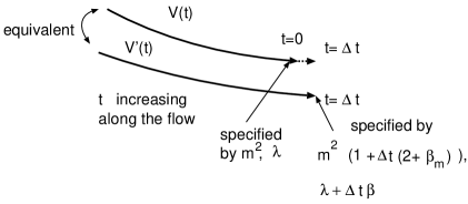
Figure 3: Original ERG flows: $(m^{2},\lambda)$ and $(m^{2}+\Delta t(2+\beta_{m}(\lambda)),\lambda+\beta(\lambda))$ specify the end points of two different but physically equivalent ERG flows.

We can also define an alternative anomalous dimension of the scalar field by

$$\tilde{\gamma}(\lambda)\equiv\frac{1}{2}\frac{\eta}{\Delta t}$$ (176)

so that Eqs. (168) imply the familiar RG equation for the Green functions:

$$\left\langle~{}\phi(p_{1})\cdots\phi(p_{2n-1})\phi~{}\right\rangle_{m^{2},\lambda}$$ (177)

$$= (1+(4n-y_{2n}-2n\tilde{\gamma})\Delta t)\left\langle~{}\phi(p_{1}\mathrm{e}^{\Delta t})\cdots\phi(p_{2n-1}\mathrm{e}^{\Delta t})\phi~{}\right\rangle_{m^{2}(\Delta t),\lambda(\Delta t)}$$

For completeness, let us write down the expressions of the alternative beta function and anomalous dimensions:

$$2\tilde{\gamma}(\lambda) \equiv \frac{-\frac{1}{2}\frac{\partial}{\partial p^{2}}\left(\int_{q}\frac{\Delta(q)}{q^{2}}A_{4}(q,-q,p,-p)\right)_{p^{2}=0}}{1-\frac{1}{2}\frac{\partial}{\partial p^{2}}\left(\int_{q}\frac{K(q)(1-K(q))}{q^{2}}\,A_{4}(q,-q,p,-p)\right)_{p^{2}=0}}$$ (178)

$$\tilde{\beta}_{m}(\lambda) \equiv \frac{1}{1-\frac{1}{2}\int_{q}\frac{K(q)(1-K(q))}{q^{4}}\,A_{4}(q,-q,0,0)}$$

$$\times\Bigg{[}\frac{1}{2}\int_{q}\Delta(q)\left(\frac{A_{4}(q,-q,0,0)}{q^{4}}-\frac{B_{4}(q,-q,0,0)}{q^{2}}\right)$$

$$-2~{}\tilde{\gamma}(\lambda)\left\{1-\frac{1}{2}\int_{q}K(q)(1-K(q))\left(\frac{B_{4}(q,-q,0,0)}{q^{2}}-\frac{A_{4}(q,-q,0,0)}{q^{4}}\right)\right\}\Bigg{]}$$

$$\tilde{\beta}(\lambda) \equiv -\frac{1}{2}\int_{q}\frac{\Delta(q)}{q^{2}}A_{6}(q,-q,0,0,0,0)$$ (180)

$$-2\tilde{\gamma}(\lambda)\left(2\lambda-\frac{1}{2}\int_{q}\frac{K(q)(1-K(q))}{q^{2}}\,A_{6}(q,-q,0,0,0,0)\right)$$

The above are significantly more complicated than those (84, 85, 86) defined using the modified ERG equation in sect. IV. But that is not the biggest drawback of the alternative definition. The biggest drawback is the lack of a scaling relation for the vertices. Let $\{\mathcal{V}_{2n}(t;p_{1},\cdots,p_{2n};m^{2},\lambda)\}$ denote the vertices on the ERG trajectory whose end point at $t=0$ is specified by $m^{2},\lambda$. Then the scaling relation would give

$$\mathcal{V}_{2n}(t;p_{1},\cdots,p_{2n};m^{2},\lambda)=\mathcal{V}_{2n}(0;p_{1},\cdots,p_{2n};m^{2}(t),\lambda(t))$$ (181)

But this is NOT the case here, simply because $\{\mathcal{V}_{2n}(0;m^{2}(t),\lambda(t))\}$ is not on the same ERG trajectory as $\{\mathcal{V}_{2n}(0;m^{2},\lambda)\}$.

Appendix C Lowest order cutoff dependence

In this appendix we compute $\epsilon(\lambda)$, $\eta(\lambda)$, $\delta\lambda(\lambda)$, $u(p;m^{2},\lambda)$, and $t(p;m^{2},\lambda)$ in sect. VII to lowest order in $\lambda$. To denote the order of expansions in $\lambda$, we use the same notation as in Appendix A.

$\epsilon$, $\eta$, and $\delta\lambda$ are determined by Eqs. (114, 115, 116). They depend on $u$, but $u$ is first order in $\lambda$, and we do not need it for the lowest order calculations. We find

$$\eta^{(2)} = \frac{1}{2}\frac{\partial}{\partial p^{2}}\int_{q}\frac{\delta K(q)}{q^{2}}\,A_{4}^{(2)}(q,-q,p,-p)\Bigg{|}_{p^{2}=0}$$ (182)

$$= 2\frac{\partial}{\partial p^{2}}\int_{q}\frac{\delta K(q)}{q^{2}}\frac{(1-K(q+p))}{(q+p)^{2}}\Bigg{|}_{p^{2}=0}=-\int_{q}\frac{\delta K(q)}{q^{2}}K^{\prime\prime}(q)$$

$$\epsilon^{(1)} = \frac{1}{2}\int_{q}\frac{\delta K(q)}{q^{4}}(-A_{4}^{(1)}(q,-q,0,0))=-\frac{1}{2}\int_{q}\frac{\delta K(q)}{q^{4}}$$ (183)

$$\delta\lambda^{(2)} = \frac{1}{2}\int_{q}\frac{\delta K(q)}{q^{2}}A_{6}^{(2)}(q,-q,0,0,0,0)=3\int_{q}\frac{\delta K(q)(1-K(q))}{q^{4}}$$ (184)

Since $\eta$ is second order in $\lambda$, we find that the anomalous dimension $\gamma$ of the scalar field is universal (i.e., independent of $K(p)$) up to order $\lambda^{2}$.

The functions $u(p;m^{2},\lambda)$ and $t(p;m^{2},\lambda)$ are determined by Eqs. (120, 121). To lowest order in $\lambda$, the equation for $u$ becomes

$$2\left(p^{2}\frac{\partial}{\partial p^{2}}+m^{2}\frac{\partial}{\partial m^{2}}\right)u^{(1)}(p;m^{2})=(\delta K(p)\beta_{m}^{(1)}+\Delta(p)\epsilon^{(1)})\frac{m^{2}}{p^{2}+m^{2}}$$ (185)

where $\beta_{m}^{(1)}$ is given by Eq. (132). Hence, we obtain

$$u^{(1)}(p;m^{2})=\frac{m^{2}}{p^{2}+m^{2}}\left(\beta_{m}^{(1)}\int_{0}^{\infty}dt\,\delta K(p\mathrm{e}^{-t})+\epsilon^{(1)}(1-K(p))\right)$$ (186)

In fact we can add an arbitrary function $c$ of $p^{2}/m^{2}$ to the above solution. But $u$ must vanish for $p^{2}<1$, and this imposes $c=0$ for $p^{2}<1$ for an arbitrary $m^{2}$. Thus, we conclude $c=0$ identically.

To lowest order in $\lambda$, the equation (121) for $t(p;m^{2},\lambda)$ gives

$$2\left(p^{2}\frac{\partial}{\partial p^{2}}+m^{2}\frac{\partial}{\partial m^{2}}\right)t^{(2)}(p;m^{2})=\beta_{m}^{(1)}u^{(1)}(p;m^{2})\frac{m^{2}}{p^{2}+m^{2}}$$ (187)

Its unique solution is given by

$$t^{(2)}(p)=\beta_{m}^{(1)}\left(\frac{m^{2}}{p^{2}+m^{2}}\right)^{2}\left(\beta_{m}^{(1)}\int_{0}^{\infty}dt^{\prime}\int_{0}^{\infty}dt\,\delta K(p\mathrm{e}^{-(t+t^{\prime})})+\epsilon^{(1)}\int_{0}^{\infty}dt(1-K(p\mathrm{e}^{-t}))\right)$$ (188)

Appendix D Spontaneous symmetry breaking

For $m^{2}<0$, we have spontaneous symmetry breaking, and the scalar field acquires a non-vanishing expectation value:

$$\left\langle~{}\phi~{}\right\rangle=M>0$$ (189)

The ERG equation is still valid irrespective of the sign of $m^{2}$ as long as

$$m^{2}>-1$$ (190)

This is because in the ERG equation the dangerous denominator $p^{2}+m^{2}$ appears always as either

$$\frac{\Delta(p)}{p^{2}+m^{2}}\quad\text{or}\quad\frac{1-K(p)}{p^{2}+m^{2}}$$ (191)

where $\Delta(p)=1-K(p)=0$ for $p^{2}<1$.

However, the perturbative calculations of the Green functions cannot be done with the propagator

$$\frac{K(p)}{p^{2}+m^{2}}$$ (192)

because the denominator vanishes at $p^{2}=-m^{2}<1$ for which $K(p)=1$. Therefore, we need to rearrange the interaction terms in the full action to get a sensible propagator. Otherwise perturbative calculations will not make sense.

Given a full action

$$S[\phi] = \frac{1}{2}\int_{p}\frac{p^{2}+m^{2}}{K(p)}\phi(p)\phi(-p)$$ (193)

$$-\sum_{n=1}^{\infty}\frac{1}{(2n)!}\int_{p_{1},\cdots,p_{2n-1}}\mathcal{V}_{2n}(p_{1},\cdots,p_{2n})\phi(p_{1})\cdots\phi(p_{2n})$$

we introduce the replacement

$$\phi(p)=\varphi(p)+M(2\pi)^{4}\delta^{(4)}(p)$$ (194)

where $\varphi$ has zero expectation value. Dropping the $\varphi$ independent constant terms, we obtain

$$S[\phi] = \varphi(0)\left(m^{2}M-\sum_{n=1}^{\infty}\frac{M^{2n-1}}{(2n-1)!}\mathcal{V}_{2n}(0,\cdots,0)\right)+\frac{1}{2}\int_{p}\frac{p^{2}+m^{2}}{K(p)}\,\varphi(p)\varphi(-p)$$ (195)

$$-\sum_{l=2}^{\infty}\frac{1}{l!}\int_{p_{1},\cdots,p_{l-1}}\varphi(p_{1})\cdots\varphi(p_{l})\sum_{n=\left[\frac{l+1}{2}\right]}^{\infty}\frac{M^{2n-l}}{(2n-1)!}\mathcal{V}_{2n}(p_{1},\cdots,p_{l},0,\cdots,0)$$

To find the propagator, we extract the coefficient of the quadratic term which is given by

$$\frac{p^{2}+m^{2}}{K(p)}-\sum_{n=1}^{\infty}\frac{M^{2n-2}}{(2n-2)!}\mathcal{V}_{2n}(p,-p,0,\cdots,0)$$ (196)

In calculating the Green functions in powers of the coupling constant $\lambda$, we regard both $m^{2}$ and $\lambda M^{2}$ as order $1$. (At tree level, $m^{2}=-\lambda M^{2}/6$.) Hence, the order $1$ contribution to the quadratic term is given by

$$C(p)\equiv\frac{p^{2}+m^{2}}{K(p)}-\sum_{n=2}^{\infty}\frac{(-\lambda M^{2})^{n-1}}{(2n-2)!}\mathcal{V}_{2n}^{(n-1)}(p,-p,0,\cdots,0)$$ (197)

where $(-\lambda)^{n-1}\mathcal{V}_{2n}^{(n-1)}$ is the tree-level vertex given by

$$\mathcal{V}_{2n}^{(n-1)}(p,-p,0,\cdots,0)=\frac{(2(n-1))!}{2^{n-1}}\left(\frac{1-K(p)}{p^{2}+m^{2}}\right)^{n-2}$$ (198)

Figure 4: $2n$-point vertex at tree-level

(See FIG. 4.) Note $\mathcal{V}_{2}=0$ at tree-level. Therefore, we obtain

$$C(p) = \frac{p^{2}+m^{2}}{K(p)}+\frac{\lambda M^{2}}{2}\sum_{n=2}^{\infty}\left(\frac{-\lambda M^{2}}{2}\frac{1-K(p)}{p^{2}+m^{2}}\right)^{n-2}$$ (199)

$$= \frac{\left(p^{2}+m^{2}+\frac{\lambda M^{2}}{2}\right)(p^{2}+m^{2})}{K(p)\left(p^{2}+m^{2}+\frac{\lambda M^{2}}{2}(1-K(p))\right)}$$

Hence, the propagator is given by

$$\frac{1}{C(p)} = \frac{K(p)}{p^{2}+m^{2}+\frac{\lambda M^{2}}{2}}\cdot\frac{p^{2}+m^{2}+\frac{\lambda M^{2}}{2}(1-K(p))}{p^{2}+m^{2}}$$

$$= \frac{1}{p^{2}+m^{2}+\frac{\lambda M^{2}}{2}}\quad\text{for}\quad p^{2}<1$$

This is well defined for any $p^{2}$, and vanishes for $p^{2}>2^{2}$ due to $K(p)$ in the numerator.

Therefore, the full action can be written as

$$S[\phi]=\frac{1}{2}\int_{p}C(p)\varphi(p)\varphi(-p)+S^{\prime}_{\text{int}}[\varphi]$$ (201)

where the interaction part is given by

$$S^{\prime}_{\text{int}}[\varphi] = \varphi(0)\left(m^{2}M-\sum_{n=1}^{\infty}\frac{M^{2n-1}}{(2n-1)!}\mathcal{V}_{2n}(0,\cdots,0)\right)$$ (202)

$$-\frac{1}{2}\int_{p}\varphi(p)\varphi(-p)\,\sum_{n=1}^{\infty}\frac{M^{2(n-1)}}{2(n-1)!}\left(\mathcal{V}_{2n}(p,-p,0,\cdots,0)-\mathcal{V}_{2n}^{(n-1)}(p,-p,0,\cdots,0)\right)$$

$$-\sum_{l=3}^{\infty}\frac{1}{l!}\int_{p_{1},\cdots,p_{l-1}}\varphi(p_{1})\cdots\varphi(p_{l})\sum_{n=\left[\frac{l+1}{2}\right]}^{\infty}\frac{M^{2n-l}}{(2n-1)!}V_{2n}(p_{1},\cdots,p_{l},0,\cdots,0)$$

This is at least of order $\lambda$, and hence perturbative calculations can be done using the propagator (D) and the above interaction action.

References

Wilson and Kogut (1974)
K. G. Wilson and
J. Kogut,
Phys. Repts. 12C,
75 (1974).
(2)
H. Sonoda, to
appear in Phys. Rev. D. (hep-th/0212302).