We use analytic and numerical methods to obtain the solution of the Q-ball equation of motion. In particular, we show that the profile function of the three-dimensional Q-ball can be accurately approximated by the symmetrized Woods-Saxon distribution.

1 Introduction

The existence of Q-balls is a general feature of scalar field theories carrying a conserved $U(1)$ charge [1, 2]. Q-balls can be understood as bound states of scalar particles and appear as stable classical solutions (nontopological solitons) carrying a rotating time dependent internal phase. They are characterized by a conserved nontopological charge $Q$ (Noether charge) which is responsible for their stability (see, for example, Refs. [3]-[4]). These features differentiate the Q-ball interaction properties from those of the topological solitons since here the charge $Q$ can take arbitrary values in a specific range, allowing for the possibility of charge transfer between solitons during the interaction process.

Up till now, comprehensive studies of these objects have been made by using either numerical simulations [3]-[5] or some analytic considerations [1, 6, 7]. Recently, in [8] the explicit relation between the energy and the charge of the Q-balls has been derived using analytic arguments. In particular, a semi-Bogomolny argument in the energy density led to a first order differential equation whose solution however, did not satisfy the correct boundary conditions and differed considerably from its exact form. In this work, we present a method to obtain an analytic form for the Q-ball profile function which is in good agreement with the numerical results.

We consider the $U(1)$ Goldstone model, given by the Lagrangian

$${\cal L}=\frac{1}{2}\partial_{\mu}\phi\,\partial^{\mu}\bar{\phi}-U(|\phi|)$$ (1)

where $\phi$ is a single complex scalar field in three spatial dimensions while the potential $U(|\phi|)$ is a function of $|\phi|$ only and has a single minimum at $\phi=0$. This is equivalent of stating that there is a sector of scalar particles (mesons) which carry $U(1)$ charge and have mass squared equal to $\frac{1}{2}U^{\prime\prime}(0)$. The corresponding energy functional is given by

$$E=\int\left(\frac{1}{2}|\partial_{t}{\phi}|^{2}+\frac{1}{2}|\nabla\phi|^{2}+U(|\phi|)\right)d^{3}x.$$ (2)

The model has a global $U(1)$ symmetry and an associated conserved Noether current $J_{\mu}$ exists whose covariant conservation $\partial^{\mu}J_{\mu}=0$ leads to the existence of the conserved Noether charge $Q$ given by

$$Q=\frac{1}{2i}\int\left(\bar{\phi}\,\partial_{t}\phi-\phi\,\partial_{t}\bar{\phi}\right)d^{3}x.$$ (3)

A stationary Q-ball solution has the form

$$\phi=e^{i\omega t}f(r)$$ (4)

where $f(r)$ is a real radial profile function which satisfies the ordinary differential equation

$$f^{\prime\prime}(r)+\frac{2}{r}f^{\prime}(r)=-\omega^{2}f(r)+U^{\prime}(f)$$ (5)

with the condition $f(\infty)=0$ and $f^{\prime}(0)=0$. This equation can either be interpreted as describing the motion of a point particle moving in a potential with friction [1], or in terms of Euclidean bounce solutions [9]. In each case the effective potential being $U_{eff}(f)=\omega^{2}f^{2}/2-U(f)$ leads to constraints on the potential $U(f)$ and the frequency $\omega$ in order for a Q-ball solution to exist. Firstly, the effective mass of $f$ must be negative. If we consider a potential $U(f)$ which is non-negative and satisfies $U(0)=U^{\prime}(0)=0$, $U^{\prime\prime}(0)=\omega_{+}^{2}>0$ then one can deduce that $\omega<\omega_{+}$. Furthermore, the minimum of $U(f)/f^{2}$ must be attained at some positive value of $f$, say $0<f_{0}<\infty$ and existence of the solution requires that $\omega>\omega_{-}$ where $\omega_{-}^{2}=2U(f_{0})/f_{0}^{2}$. Hence, Q-balls exist for all $\omega$ in the range $\omega_{-}<|\omega|<\omega_{+}$.

Then, the charge and the energy of a stationary Q-ball solution simplify to

$$Q = 4\pi\omega\int r^{2}\,f^{2}(r)\,dr$$ (6)

$$E = 4\pi\int\left(\frac{1}{2}\,\omega^{2}f^{2}(r)+\frac{1}{2}\,f^{\prime}{}^{2}(r)+U(f)\right)r^{2}\,dr.$$ (7)

It has been observed using numerical and analytic methods that the classical stability of a Q-ball is related with the dependence of its charge on the internal frequency $\omega$. For small internal frequency, close to its minimal value $\omega_{-}$, the profile function is almost constant which implies that the charge (6) is large and this corresponds to the so-called thin-wall approximation. On the other hand, for large internal frequency (close to its maximal value $\omega_{+}$) the profile function (and thus the charge) tends to zero and this corresponds to the thick-wall approximation. In fact, for $\omega\rightarrow\omega_{+}$, the behavior of the charge $Q$ depends on the particular form of the potential and the number of dimensions [7]. In the case studied here we show that $Q\rightarrow\infty$ as $\omega\rightarrow\omega_{+}$.

The choice of the potential is not unique; the standard requirement is that the function $U(f)/f^{2}$ has a local minimum at some value of $f$ different from zero. For simplicity, we consider the following form

$$U(f)=f^{2}\left(1+(1-f^{2})^{2}\right)$$ (8)

which implies that in terms of the earlier notation we have that $\omega_{+}=2$ and $\omega_{-}=\sqrt{2}$, and therefore stable Q-balls exist for $\sqrt{2}<\omega<2$. In this case, the energy-charge dependence of the Q-balls, obtained in [8] using a semi-Bogomolny argument, is given by the analytic expression

$$E_{{}_{Bog}}\!\!\!\! = \!\!\!\!\sqrt{2}\,Q_{{}_{Bog}}+\frac{3^{2/3}\pi^{1/3}}{2^{7/6}}\,Q_{{}_{Bog}}^{2/3}+\frac{5\pi^{2/3}}{2^{11/6}3^{2/3}}\,Q_{{}_{Bog}}^{1/3}-\frac{\pi\left(4+3\pi^{2}\right)}{36\sqrt{2}}+\frac{\pi^{4/3}\left(17-216\pi^{2}\right)}{2592~{}2^{1/6}~{}3^{1/3}}\ Q_{{}_{Bog}}^{-1/3}$$ (9)

$$\!\!\!\!+\frac{\pi^{5/3}\left(20-54\pi^{2}+27\pi^{4}\right)}{1944~{}2^{5/6}~{}3^{2/3}}\,Q_{{}_{Bog}}^{-2/3}+O\left(Q_{{}_{Bog}}^{-1}\right).$$

For large $Q$, the above equation corresponds to the upper energy bound. The same result can be obtained by representing the Q-ball profile function by the Woods-Saxon distribution (ie a generalization of the semi-Bogomolny solution) as presented in [8].

Let us emphasize that neither the semi-Bogomolny nor the Woods-Saxon ansatz describe accurately the Q-ball profile function. In particular, in both cases the derivative of the profile function at the origin is non-zero (that is, different from the required boundary conditions) while the corresponding profile function differs from the exact one obtained by solving numerically the equation of motion. In the next section, we show that the symmetrized Woods-Saxon distribution describes accurately the Q-ball profile function and satisfies the correct boundary conditions.

2 Equation of Motion

The Q-ball equation of motion (5) for the specific potential (8) is given by

$$f^{\prime\prime}(r)+\frac{2}{r}\,f^{\prime}(r)=\left(4-\omega^{2}\right)f(r)-8f^{3}(r)+6f^{5}(r)$$ (10)

and satisfies the boundary conditions $f^{\prime}(0)=0$, $f(\infty)=0$. For large values of the argument $r$ the nonlinear terms in (10) can be neglected and we get the asymptotic behaviour $f(r)\sim\exp(-\sqrt{4-\omega^{2}}\,r).$ The exact solution of (10) should contain only one free parameter $\omega$ so that the charge $Q$ the energy $E$ and the initial value $f(0)$ should in principle be expressed as functions of this parameter. Since equation (10) is too complicated to be tackled by analytic methods, we shall seek a suitable ansatz for the profile function and search for relations connecting $E$,$Q$ and $f(0)$ with $\omega$.

As mentioned earlier, a test profile of the Woods-Saxon type cannot reasonably approximate the Q-ball solution since it fails to satisfy the correct boundary conditions. Nevertheless, it implies an energy-charge relation (9) which holds remarkably well for a wide range of energies, a fact that certainly requires some further investigation. A more general test function that satisfies the correct boundary conditions and has the correct asymptotic behaviour is given by the symmetrized Woods-Saxon distribution

$$f(r)=\frac{c}{\sqrt{1+c_{1}\cosh\left(\alpha r\right)}}\ \cdot$$ (11)

The values of the arbitrary parameters $c$, $c_{1}$ and $\alpha$ can then be determined by fitting the data of the numerically solved (10). Having done that, we got a very satisfactory agreement in all cases. It is interesting to realize that $f(r)$ satisfies the following differential equation

$$f^{\prime\prime}(r)+\frac{2}{r}f^{\prime}(r)=\frac{\alpha^{2}}{4}\left(1-\frac{4}{ar}\right)f(r)-\frac{\alpha^{2}}{c^{2}}\left(1-\frac{1}{ar}\right)f^{3}(r)+\frac{3\alpha^{2}}{4c^{4}}\left((1-c_{1}^{2})+\frac{2}{3}\frac{c_{1}^{2}}{\alpha r}~{}\right)f^{5}(r)+O\left(f^{7}\right)$$ (12)

which in the limit $ar\gg 4$ looks exactly like (10). It is then quite reasonable to expect that there must be a critical value of $r=r_{c}$ beyond which the following equations must approximately hold true:

$$\frac{\alpha^{2}}{4}\left(1-\frac{4}{\alpha r_{c}}\right)\simeq 4-\omega^{2}$$ (13)

$$\frac{\alpha^{2}}{c^{2}}\left(1-\frac{1}{\alpha r_{c}}\right)\simeq 8$$ (14)

$$\frac{3\alpha^{2}}{4c^{4}}\left((1-c_{1}^{2})+\frac{2}{3}\frac{c_{1}^{2}}{\alpha r_{c}}~{}\right)\simeq 6\ \cdot$$ (15)

The thin-wall approximation is reached when $c_{1}\rightarrow 0$ so we will assume that $c_{1}<1$ and we shall neglect the last term in the left hand side of (15). Then the system above gives the approximate solutions

$$c \simeq \sqrt{\frac{2}{3}}\sqrt{1-c_{1}^{2}}\sqrt{1+\sqrt{1-\frac{3}{8}\frac{4-\omega^{2}}{1-c_{1}^{2}}}}$$ (16)

$$\alpha \simeq \frac{4\sqrt{2}}{3}\sqrt{1-c_{1}^{2}}\left(1+\sqrt{1-\frac{3}{8}\frac{4-\omega^{2}}{1-c_{1}^{2}}}\right)$$ (17)

$$\alpha r_{{}_{c}} \simeq \frac{1+\sqrt{1-\frac{3}{8}\frac{4-\omega^{2}}{1-c_{1}^{2}}}}{-\frac{1}{2}+\sqrt{1-\frac{3}{8}\frac{4-\omega^{2}}{1-c_{1}^{2}}}}\ \cdot$$ (18)

A comparison with values obtained by a direct fit shows that the relations above are quite good. In fact, equation (16) is excellent, while equation (17) gives the right shape but the actual values for $\alpha$ are on the average $10\%$ higher than expected, implying a faster drop of the profile function. Note that both $c$ and $a$ are slowly varying functions of $\omega$.

The equation of motion (10) can be written as:

$$\frac{d}{dr}\left(\frac{1}{2}\,f^{\prime}{}^{2}(r)+\frac{1}{2}\,\omega^{2}f^{2}(r)-U(f)\right)=-\frac{2}{r}\,f^{\prime}{}^{2}(r)\ \cdot$$ (19)

In the absence of the friction term, equation (19) would simply imply the conservation of energy for the corresponding mechanical problem. In the presence of friction and upon integrating (19) we get that the initial potential energy equals the work done by friction. This relation can be used to provide a further constraint on the form of (11)

$$\frac{1}{2}\,\omega^{2}f^{2}(0)-U\left(f(0)\right)=-2\int_{0}^{\infty}\frac{\,f^{\prime}{}^{2}(r)}{r}\,dr\ \cdot$$ (20)

Recall that $f(0)=c/\sqrt{1+c_{1}}$. Finally, using the symmetrized Woods-Saxon distribution (11), the charge (6) and the energy (7) of the Q-ball can be explicitly evaluated in terms of the parameters $c$, $c_{1}$ and $\alpha$:

$$Q = 4\pi\omega\,\frac{c^{2}}{3\alpha^{3}\sqrt{1-c_{1}^{2}}}\,\cosh^{-1}\left(\frac{1}{c_{1}}\right)\left(\pi^{2}+\cosh^{-1}\left(\frac{1}{c_{1}}\right)^{2}\right),$$ (21)

$$E = 4\pi\left[\frac{\alpha^{2}+4\left(4+\omega^{2}\right)}{8}\,I_{0}-\left(2+\frac{\alpha^{2}}{4c^{2}}\right)I_{1}+\left(1+\frac{\alpha^{2}}{8c^{4}}\left(1-c_{1}^{2}\right)\right)I_{2}\right],$$ (22)

where the integrals $I_{0}$, $I_{1}$ and $I_{2}$ are given by

$$I_{0} = \frac{Q}{4\pi\omega},$$ (23)

$$I_{1} = c^{2}I_{0}+c^{2}c_{1}\frac{d}{dc_{1}}I_{0},$$ (24)

$$I_{2} = c^{4}I_{0}+2c^{4}c_{1}\frac{d}{dc_{1}}I_{0}+\frac{1}{2}c^{4}c_{1}^{2}\frac{d^{2}}{dc_{1}^{2}}I_{0}\ \cdot$$ (25)

It is readily seen that the actual values for $Q$ and $E$ depend strongly on the value of $c_{1}$ especially for small values of $c_{1}$. In this region, $c_{1}$ can be eliminated in favour of $Q$ to get

$$E = \left(\frac{1}{\omega}+\frac{\omega}{2}\right)Q+\frac{24+3\,\alpha^{2}}{16\,\omega}\left(q\omega\right)^{\frac{1}{3}}\,{Q}^{\frac{2}{3}}+\frac{24+3\,\alpha^{2}}{8\omega\,}\left(q\omega\right)^{\frac{2}{3}}\,{Q}^{\frac{1}{3}}-\frac{\left(8+\,\alpha^{2}\right)\,{\pi}^{2}}{8\,\omega}q\omega~{}+{{O}(Q}^{-\frac{1}{3}}{)\quad}$$ (26)

where

$$q=\frac{4\pi c^{2}}{3\alpha^{3}}\ \cdot$$ (27)

It is interesting to see that the leading terms of (26) are identical to those of (9) for $\alpha=2\sqrt{2}$, $c=1$, $\omega=\sqrt{2}$. Taking into account the fact that $\alpha$ and $c$ are slowly varying functions of $\omega$ helps to explain the wide range of applicability of (9).

As a result, the parameters $c$, $c_{1}$, $\alpha$ and $\omega$ for specific values of the charge $Q$ can be uniquely determined by solving the system of equations: (16), (20), (21), and (22) provided that the energy-charge dependence of the Q-ball is given by (9). We expect the values obtained that way to be quite accurate as long as (9) remains reasonably accurate. In practice, this means that $Q\gtrsim 16$, a value far distant from the values normally associated with the region of the thin-wall approximation. In Table 1 the values of the arbitrary constants in (11) are presented for different values of $Q$ (or $\omega$). That way, the initial value $f(0)$ can be determined explicitly; a comparison with values obtained numerically show that the symmetrized Woods-Saxon distribution describes accurately the Q-ball profile function.

$Q$	$\omega$	$c$	$c_{1}$	$\alpha$	$f(0)$	$f(0)_{num}$
23.68	1.79	1.097	0.12	2.66	1.037	1.024
35	1.72	1.087	0.068	2.60	1.052	1.055
61.6	1.64	1.068	0.0243	2.54	1.056	1.065
149.3	1.57	1.049	0.0031	2.53	1.048	1.056

Table 1: Values of the parameters $c$, $c_{1}$, $\alpha$ and $f(0)$ obtained from $(\ref{WSsym})$ and numerically ($f(0)_{num}$) for different values of $\omega$.

Finally, Figure 1 presents the profile function obtained analytically and numerically for $\omega=1.64$. Figure 2 presents the values of the profile function at the origin for different $\omega$ obtained numerically and analytically.

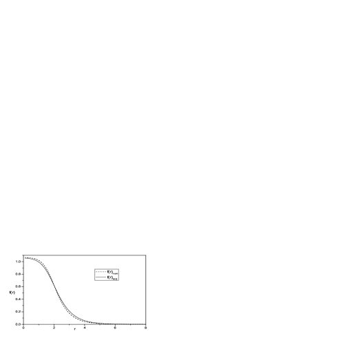
Figure 1: The profile function $f(r)$ as a function of $r$ for $\omega=1.64$

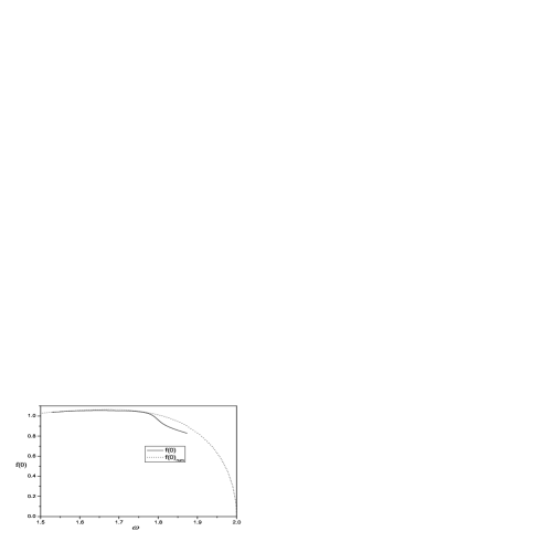
Figure 2: The frequency dependence of the profile function at the origin $f(0)$.

3 Conclusions

In this work, the basic properties of the Q-ball profile function have been extensively studied by means of mainly analytic methods. In particular, it has been shown that the profile function can be accurately approximated by the symmetrized Woods-Saxon distribution, while the corresponding energy and charge can be explicitly evaluated. The approach presented here might prove to be particularly useful in understanding the basic properties of Q-balls such as existence, small vibrations and stability. We believe that a similar line of argument can be applied to study the profile function and the energy-charge dependence in other types of potentials. In fact, we expect that the symmetrized Woods-Saxon distribution will accurately describe all types of Q-balls independently of the exact form of the scalar potential. Work in this direction is currently in progress.

References

- [1] S. Coleman, Nucl. Phys. B 262, 263 (1985)
- [2] T.D. Lee, Particle Physics and Introduction to Field Theory, Harwood, London (1981)
- [3] J.K. Drohm, L.P. Yok, Y.A. Simonov, J.A. Tyon and V.I. Veselov, Phys. Lett. B 101, 204 (1981)
- [4] T.I. Belova and A.E. Kudryavtsev, JETP 68, 7 (1989)
- [5] M. Axenides, S. Komineas, L. Perivolaropoulos and M. Floratos, Phys. Rev. D 61, 085006 (2000)
- [6] T. Multamaki and I. Vilja, Nucl. Phys. B 574, 139 (2002); hep-ph/9908446
- [7] F. Paccetti Correia and M.G. Schmidt, Eur. Phys. J. C 21, 181 (2001); hep-th/0103189
- [8] T. Ioannidou, V. Kopeliovich and N.D. Vlachos, Energy-Charge Dependence for the Q-balls, (2003); hep-th/0302013
- [9] A. Kusenko, Phys. Lett. B 404, 285 (1997)
- [10] H.T. Davis, Introduction to Nonlinear Differential and Integral Equations, Dover Publications (1962)