Abstract
A localized configuration is found in the 5D bulk-boundary theory on an $S_{1}/Z_{2}$ orbifold model of Mirabelli-Peskin. A bulk scalar and the extra (fifth) component of the bulk vector constitute the configuration. ${\cal N}=1$ SUSY is preserved. The effective potential of the SUSY theory is obtained using the background field method. The vacuum is treated in a general way by allowing its dependence on the extra coordinate. Taking into account the supersymmetric boundary condition, the 1-loop full potential is obtained. The scalar-loop contribution to the Casimir energy is also obtained. Especially we find a new type which depends on the brane configuration parameters besides the $S_{1}$ periodicity parameter.

PACS NO:  11.10.Kk, 11.27.+d, 12.60.Jv, 12.10.-g, 11.25.Mj, 04.50.+h
Key Words: Mirabelli-Peskin model, supersymmetric boundary condition, SUSY effective potential, bulk-boundary theory.

1 Introduction Through the development of the recent several years, it looks that the higher-dimensional approach begins to obtain the citizenship as an important building tool in constructing a unified theory. Among many ideas in this approach, the system of bulk and boundary theories becomes a fascinating model of the unification. The boundary is regarded as our 4D world. It is inspired by the M, string and D-brane theories[1]. One pioneering paper, giving a concrete field-theory realization, is that by Mirabelli and Peskin[2]. They consider 5D supersymmetric Yang-Mills theory with a boundary matter. The boundary couplings with the bulk world are uniquely fixed by the SUSY requirement. They demonstrated some consistency of the bulk and boundary quantum effects by calculating self-energy of the scalar matter field. Here we examine the vacuum configuration and the effective potential.

Contrary to the motivation of ref.[2], we do not seek the SUSY breaking mechanism, rather we make use of the SUSY-invariance properties in order to make the problem as simple as possible. The SUSY symmetry is so restrictive that we only need to calculate some small portion of all possible diagrams.

In the calculation of the effective potential of the 5D model, we recall that of the Kaluza-Klein model. The dynamics quantumly produces the effective potential which describes the Casimir effect[3, 4]. The situation, however, is different from the present case in the following points: 1) the 4D reduction mechanism; 2) Z₂-symmetry; 3) treatment of the vacuum with respect to the extra-coordinate dependence; 4) supersymmetry; 5) characteristic length scales. We will compare the present result with the KK case.

2 Mirabelli-Peskin Model Let us consider the 5 dimensional flat space-time with the signature (-1,1,1,1,1). The space of the fifth component is taken to be ($S_{1}$), with the periodicity $2l$, and has the $Z_{2}$-orbifold condition.

$${x^{5}}\rightarrow{x^{5}}+2l\ (\mbox{periodicity}){\quad,}\quad{x^{5}}\leftrightarrow-{x^{5}}\ (Z_{2}\mbox{-symmetry}){\quad.}$$ (1)

We take a 5D bulk theory ${\cal L}_{bulk}$ which is coupled with a 4D matter theory ${\cal L}_{bnd}$ on a ”wall” at ${x^{5}}=0$ and with ${\cal L}^{\prime}_{bnd}$ on the other ”wall” at ${x^{5}}=l$. The boundary Lagragians are, in the bulk action, described by the delta-functions along the extra axis $x^{5}$.

$$S=\int d^{5}x\{{\cal L}_{blk}+\delta(x^{5}){\cal L}_{bnd}+\delta(x^{5}-l){{\cal L}^{\prime}}_{bnd}+\mbox{periodic part}\}{\quad.}$$ (2)

We consider both bulk and boundary quantum effects.

The bulk dynamics is given by the 5D super YM theory which is made of a vector field $A^{M}\ (M=0,1,2,3,5)$, a scalar field $\Phi$, a doublet of symplectic Majorana fields $\lambda^{i}\ (i=1,2)$, and a triplet of auxiliary scalar fields $X^{a}\ (a=1,2,3)$:

$${\cal L}_{SYM}=-{\frac{1}{2}}{\rm tr\,}{F_{MN}}^{2}-{\rm tr\,}(\nabla_{M}\Phi)^{2}-i{\rm tr\,}({\bar{\lambda}}_{i}\gamma^{M}\nabla_{M}\lambda^{i})+{\rm tr\,}(X^{a})^{2}+{\rm tr\,}({\bar{\lambda}}_{i}[\Phi,\lambda^{i}]){\quad,}$$ (3)

where all bulk fields are the adjoint representation (its suffixes: $\alpha,\beta,\cdots$) of the gauge group $G$. The bulk Lagrangian ${\cal L}_{SYM}$ is invariant under the 5D SUSY transformation. This system has the symmetry of 8 real super charges. As the 5D gauge-fixing term, we take the Feynman gauge:

$${\cal L}_{gauge}=-{\rm tr\,}(\partial_{M}A^{M})^{2}=-{\frac{1}{2}}(\partial_{M}A^{M}_{~{}\alpha})^{2}{\quad.}$$ (4)

The corresponding ghost Lagrangian is given by

$${\cal L}_{ghost}=-2\,{\rm tr\,}\partial_{M}{\bar{c}}\cdot\nabla^{M}(A)c=-2\,{\rm tr\,}\partial_{M}{\bar{c}}\cdot(\partial^{M}c+ig[A^{M},c]){\quad,}$$ (5)

where $c$ and ${\bar{c}}$ are the complex ghost fields. We take the following bulk action.

$${\cal L}_{blk}={\cal L}_{SYM}+{\cal L}_{gauge}+{\cal L}_{ghost}{\quad.}$$ (6)

It is known that we can consistently project out ${\cal N}=1$ SUSY multiplet, which has 4 real super charges, by assigning $Z_{2}$-parity to all fields in accordance with the 5D SUSY. A consistent choice is given as:  $P=+1$ for $A^{m},\lambda_{L},X^{3}$; $P=-1$ for $A^{5},\Phi,\lambda_{R},X^{1},X^{2}$ ($m=0,1,2,3$). Then ($A^{m},\lambda_{L},X^{3}-\nabla_{5}\Phi$) constitute an ${\cal N}=1$ vector multiplet. Especially ${\cal D}\equiv X^{3}-\nabla_{5}\Phi$ plays the role of D-field on the wall. We introduce one 4 dim chiral multiplet ($\phi,\psi,F$) on the ${x^{5}}=0$ wall and the other one ($\phi^{\prime},\psi^{\prime},F^{\prime}$) on the ${x^{5}}=l$ wall: complex scalar fields $\phi,\phi^{\prime}$, Weyl spinors $\psi,\psi^{\prime}$, and auxiliary fields of complex scalar $F,F^{\prime}$. These are the simplest matter candidates and were taken in the original theory[2]. Using the ${\cal N}=1$ SUSY property of the fields ($A^{m},\lambda_{L},X^{3}-\nabla_{5}\Phi$), we can find the following bulk-boundary coupling on the ${x^{5}}=0$ wall.

$${\cal L}_{bnd}=-\nabla_{m}\phi^{\dagger}\nabla^{m}\phi-\psi^{\dagger}i{\bar{\sigma}}^{m}\nabla_{m}\psi+F^{\dagger}F+\sqrt{2}ig({\bar{\psi}}{\bar{\lambda}}_{L}\phi-\phi^{\dagger}\lambda_{L}\psi)+g\phi^{\dagger}{\cal D}\phi{\quad,}$$ (7)

where $\nabla_{m}\equiv\partial_{m}+igA_{m},\ {\cal D}=X^{3}-\nabla_{5}\Phi$. We take the fundamental representation for $\phi,\phi^{\dagger}$. The quadratic (kinetic) terms of the vector $A^{m}$, the gaugino spinor $\lambda_{L}$ and the ’auxiliary’ field ${\cal D}=X^{3}-\nabla_{5}\Phi$ are in the bulk world. In the same way we introduce the coupling between the matter fields ($\phi^{\prime},\psi^{\prime},F^{\prime}$) on the ${x^{5}}=l$ wall and the bulk fields: ${\cal L}^{\prime}_{bnd}=(\phi\rightarrow\phi^{\prime},\psi\rightarrow\psi^{\prime},F\rightarrow F^{\prime}in\mbox{(\ref{mp7})})$. We note the interaction between the bulk fields and the boundary ones is definitely fixed from SUSY.

3 SUSY Boundary Condition, Background Expansion and Generalized vacuum First we point out an important fact about the SUSY effective potential. The 1-loop SUSY effective potential can be calculated only by the scalar loop up to the $F$- and $D$-independent terms in the off-shell treatment. If we trace the origin of this phenomenon, it is simply that the auxiliary fields have the higher physical dimension of $M^{2}$. They cannot have the Yukawa coupling with fermions and vectors. F and D-dependence in the SUSY effective potential is very important to determine the vacuum behaviour. The above fact means that $dV^{eff}_{1-loop}/dD$ ( or $dV^{eff}_{1-loop}/dF$ ) is definitely determined only by the scalar loop. Miller[6, 7], using the above fact, obtained F-tadpole or D-tadpole [8] (F and D-tadpole correspond to $dV^{eff}_{1-loop}/dF$ and $dV^{eff}_{1-loop}/dD$, respectively.) in general 4D SUSY theories. He noticed, if the theory preserve SUSY at the quantum level, the $F$ and $D$-independent parts in $V^{eff}_{1-loop}$ can be obtained, instead of calculating diagrams, by a boundary condition on the effective potential. This is because, in the SUSY-preserving case, the effective potential should satisfy: $V^{eff}(F=0,D=0)=0$ –supersymmetric boundary condition–. He confirmed the correctness by comparing his results with the results in the ordinary method. (See ref.[9] for an application to unified models.) We follow Miller’s idea.

Hence we may put, for the purpose of obtaining the 1-loop SUSY effective potential, the following conditions:

$$A^{m}=0\ (m=0,1,2,3){\quad,}\quad\lambda^{i}={\bar{\lambda}}^{i}=0{\quad,}\quad\psi=0{\quad,}\quad\psi^{\prime}=0{\quad,}\quad\lambda_{L}=0{\quad.}$$ (8)

Here the extra (fifth) component of the bulk vector $A^{5}$ does not taken to be zero because it is regarded as a 4D scalar on the wall. The extra coordinate ${x^{5}}$ is regarded as a parameter. Then ${\cal L}_{blk}$ reduces to

$${\cal L}^{red}_{blk}[\Phi,X^{3},A_{5}]={\rm tr\,}\left\{-\partial_{M}\Phi\partial^{M}\Phi+X^{3}X^{3}-\partial_{M}A_{5}\partial^{M}A_{5}+2g(\partial_{5}\Phi\times A_{5})\Phi\right.$$

$$\left.-g^{2}(A_{5}\times\Phi)(A_{5}\times\Phi)-2\partial_{M}{\bar{c}}\cdot\partial^{M}c-2ig\partial_{5}{\bar{c}}\cdot[A^{5},c]\right\}+\mbox{irrel. terms}{\quad,}$$ (9)

where we have dropped terms of $2{\rm tr\,}X^{1}X^{1}=X^{1}_{\alpha}X^{1}_{\alpha},2{\rm tr\,}X^{2}X^{2}=X^{2}_{\alpha}X^{2}_{\alpha}$ as ’irrelevant terms’ because they decouple from other fields. (Note ${\rm tr\,}(\partial_{5}\Phi\times A_{5})\Phi=(1/2)f_{{\alpha\beta}\gamma}\partial_{5}\Phi_{\alpha}A_{5\beta}\Phi_{\gamma}$.) While ${\cal L}_{bnd}$, on the ${x^{5}}=0$ wall, reduces to

$${\cal L}^{red}_{bnd}[\phi,\phi^{\dagger},X^{3}-\nabla_{5}\Phi]=-\partial_{m}\phi^{\dagger}\partial^{m}\phi+g(X^{3}_{\alpha}-\nabla_{5}\Phi_{\alpha})\phi^{\dagger}_{\beta^{\prime}}(T^{\alpha})_{{\beta^{\prime}}{\gamma^{\prime}}}\phi_{\gamma^{\prime}}+\mbox{irrl. terms}{\quad,}$$ (10)

where we have dropped $F^{\dagger}F$-terms as the irrelevant terms. ${\alpha^{\prime}},{\beta^{\prime}}$ are the suffixes of the fundamental representation. In the same way, we obtain ${{\cal L}^{red}_{bnd}}^{\prime}[\phi^{\prime},{\phi^{\prime}}^{\dagger},X^{3}-\nabla_{5}\Phi]$ on the ${x^{5}}=l$ wall.

Now we take the background-field method[10, 11, 12] to obtain the effective potential. We expand all scalar fields ($\Phi,X^{3},A_{5};\phi,\phi^{\prime}$), except ghosts, into the quantum fields (which are denoted again by the same symbols) and the background fields ($\varphi,\chi^{3},a_{5};\eta,\eta^{\prime}$).

$$\Phi\rightarrow\varphi+\Phi\ ,\ X^{3}\rightarrow\chi^{3}+X^{3}\ ,\ A_{5}\rightarrow a_{5}+A_{5}\ ,\ \phi\rightarrow\eta+\phi\ ,\ \phi^{\prime}\rightarrow\eta^{\prime}+\phi^{\prime}\ ,$$ (11)

We treat the ghosts $c$ and ${\bar{c}}$ as quantum fields.

We state a new point in the present use of the background-field method. Usually we take the following procedure in order to obtain the vacuum[13].

[Ordinary procedure of the vacuum search]
1) First we obtain the effective potential assuming the scalar property of the vacuum (as described in (8)) and the constancy of the scalar vacuum expectation values.
2) Then we take the minimum of the effective potential.

In the present case, however, we have the extra coordinate ${x^{5}}$. We have ”freedom” in the treatment of the vacuum expectation values because ${x^{5}}$ is regarded as a simple parameter. We require that the background fields may be constant only in 4D world, not necessarily in 5D world. We may allow the background fields to depend on the extra coordinate $x^{5}$. This standpoint gives us an interesting possibility to the higher dimensional model and generalizes the vacuum of the system.

When the background fields ($\varphi,\chi^{3},a_{5};\eta,\eta^{\prime}$) satisfy the field equations derived from (9) and (10), we say they satisfy the on-shell condition. The equations are , in the order of the variations $(\delta\Phi_{\alpha},\delta A_{5\alpha},\delta\chi^{3}_{\alpha},\delta\phi^{\dagger}_{\alpha^{\prime}},\delta\phi^{\prime{\dagger}}_{\alpha^{\prime}})$, respectively given as,

$$\partial_{5}Z_{\alpha}+g(Z\times a_{5})_{\alpha}=0{\quad,}\quad{\partial_{5}}^{2}a_{5\alpha}-g(\varphi\times Z)_{\alpha}=0{\quad,}$$

$$\chi^{3}_{\alpha}+g\{\delta({x^{5}})\eta^{\dagger}T^{\alpha}\eta+\delta({x^{5}}-l)\eta^{\prime{\dagger}}T^{\alpha}\eta^{\prime}\}=0{\quad,}$$

$$d_{\beta}(T^{\beta}\eta)_{\alpha^{\prime}}=0{\quad,}\quad d_{\beta}(T^{\beta}\eta^{\prime})_{\alpha^{\prime}}=0{\quad,}$$

with the definition:

$$Z_{\alpha}\equiv-\partial_{5}\varphi_{\alpha}+g(a_{5}\times\varphi)_{\alpha}-g\{\delta({x^{5}})\eta^{\dagger}T^{\alpha}\eta+\delta({x^{5}}-l)\eta^{\prime{\dagger}}T^{\alpha}\eta^{\prime}\}{\quad,}$$

$$d_{\alpha}\equiv\chi^{3}_{\alpha}-\nabla_{5}\varphi_{\alpha}=(\chi^{3}-\partial_{5}\varphi+ga_{5}\times\varphi)_{\alpha}{\quad,}$$ (12)

where we assume, based on the standpoint of the previous paragraph, $\varphi=\varphi({x^{5}}),\chi^{3}=\chi^{3}({x^{5}}),a_{5}=a_{5}({x^{5}}),\eta=\mbox{const},\eta^{\prime}=\mbox{const}$. The third equation guarantees $Z_{\alpha}=d_{\alpha}$. In the above derivation, we use the fact that total divergences, in the action, vanish from the periodicity condition. Because we seek the effective potential (an off-shell quantity), we generally do not need to assume the above on-shell condition.

The quadratic part w.r.t. the quantum fields ($\Phi,X^{3},A_{5};\phi,\phi^{\prime}$) give us the 1-loop quantum effect. This part is given as

$${\cal L}^{2}_{blk}[\Phi,A_{5},X^{3}]={\rm tr\,}\,\{-\partial_{M}\Phi\partial^{M}\Phi+X^{3}X^{3}-\partial_{M}A_{5}\partial^{M}A_{5}\}$$

$$+2g\,{\rm tr\,}\left[(\partial_{5}\varphi\times A_{5})\Phi+(\partial_{5}\Phi\times a_{5})\Phi+(\partial_{5}\Phi\times A_{5})\varphi\right]$$

$$-2g^{2}{\rm tr\,}\left[(a_{5}\times\varphi)(A_{5}\times\Phi)\right]-g^{2}{\rm tr\,}(a_{5}\times\Phi+A_{5}\times\varphi)^{2}$$

$$-2{\rm tr\,}\,\{\partial_{M}{\bar{c}}\cdot\partial^{M}c+ig\partial_{5}{\bar{c}}\cdot[a_{5},c]\}\ ,$$

$${\cal L}^{2}_{bnd}=-\partial_{m}\phi^{\dagger}\partial^{m}\phi+gd_{\alpha}\phi^{\dagger}T^{\alpha}\phi-ig^{2}[A_{5},\Phi]_{\alpha}\eta^{\dagger}T^{\alpha}\eta$$

$$+g(X^{3}_{\alpha}-\partial_{5}\Phi_{\alpha}-ig[a_{5},\Phi]_{\alpha}-ig[A_{5},\varphi]_{\alpha})(\eta^{\dagger}T^{\alpha}\phi+\phi^{\dagger}T^{\alpha}\eta)\ ,$$

$${{\cal L}^{2}_{bnd}}^{\prime}=\{\phi\rightarrow\phi^{\prime},\ \eta\rightarrow\eta^{\prime}\ \mbox{in }{\cal L}^{2}_{bnd}\}{\quad,}$$ (13)

where $d_{\alpha}=\chi^{3}_{\alpha}-\nabla_{5}\varphi_{\alpha}$ is the background (4 dimensional) D-field and $\phi^{\dagger}T^{\gamma}\phi\equiv\phi^{\dagger}_{\alpha^{\prime}}(T^{\gamma})_{{\alpha^{\prime}}{\beta^{\prime}}}\phi_{\beta^{\prime}}$. Now we can integrate out the auxiliary field $X^{3}_{\alpha}$ in ${\cal L}^{2}_{blk}+\delta(x^{5}){\cal L}^{2}_{bnd}+\delta(x^{5}-l){{\cal L}^{2}_{bnd}}^{\prime}$. We obtain the final ”1-loop Lagrangian”, necessary for the present purpose, as

$$S^{(2)}[\Phi,A_{5};\phi]=\int d^{5}X\left[{\cal L}_{blk}^{2}|_{X^{3}=0}-\delta(x^{5})\partial_{m}\phi^{\dagger}\partial^{m}\phi\right.$$

$$\left.+\delta(x^{5})\{gd_{\alpha}(\phi^{\dagger}T^{\alpha}\phi)-g\partial_{5}\Phi_{\alpha}(\eta^{\dagger}T^{\alpha}\phi+\phi^{\dagger}T^{\alpha}\eta)-\frac{g^{2}}{2}\delta(0)(\eta^{\dagger}T^{\alpha}\phi+\phi^{\dagger}T^{\alpha}\eta)^{2}\}\right]{\quad,}$$ (14)

where $\delta(x^{5}-l)$ part is dropped because we need not to consider the quantum propagation in the ${x^{5}}=l$ brane.

4 Mass-Matrix and the Localized Background Configuration We are now ready for the full ( with respect to the coupling order) calculation of the 1-loop (we call this ”1-loop full”) effective potential. The ”1-loop action” can be expressed as

$$S^{(2)}=S^{ghost}+S^{free}+\int d^{5}X$$

$$\times{\frac{1}{2}}\left(\begin{array}[]{cccc}\phi^{\dagger}_{\alpha^{\prime}}&\phi_{\alpha^{\prime}}&\Phi_{\alpha}&A_{5\alpha}\end{array}\right){\left(\begin{array}[]{cc}\left(\begin{array}[]{cc}M_{\phi^{\dagger}\phi}&M_{\phi^{\dagger}\phi^{\dagger}}\\ M_{\phi\phi}&M_{\phi\phi^{\dagger}}\\ \end{array}\right)_{{\alpha^{\prime}}{\beta^{\prime}}}&\left(\begin{array}[]{cc}M_{\phi^{\dagger}\Phi}&0\\ M_{\phi\Phi}&0\end{array}\right)_{{\alpha^{\prime}}\beta}\\ \left(\begin{array}[]{cc}M_{\Phi\phi}&M_{\Phi\phi^{\dagger}}\\ 0&0\end{array}\right)_{\alpha{\beta^{\prime}}}&\left(\begin{array}[]{cc}M_{\Phi\Phi}&M_{\Phi A_{5}}\\ M_{A_{5}\Phi}&M_{A_{5}A_{5}}\end{array}\right)_{\alpha\beta}\end{array}\right)}\left(\begin{array}[]{c}\phi_{\beta^{\prime}}\\ \phi^{\dagger}_{\beta^{\prime}}\\ \Phi_{\beta}\\ A_{5\beta}\end{array}\right),$$ (30)

$$S^{ghost}=-\int d^{5}X\left[\partial_{M}{\bar{c}}_{\alpha}\cdot\partial^{M}c_{\alpha}+igf_{{\alpha\beta}\gamma}\partial_{5}{\bar{c}}_{\alpha}\cdot a_{5\beta}c_{\gamma}\right]\quad$$

$$S^{free}={\int d^{5}X}\left[{\rm tr\,}\,\{-\partial_{M}\Phi\partial^{M}\Phi-\partial_{M}A_{5}\partial^{M}A_{5}\}-\delta({x^{5}})\partial_{m}\phi^{\dagger}\partial^{m}\phi\right],$$ (31)

where $S^{ghost}$ is decoupled from others, and the components $M^{\prime}$s are read from (14).

Now we restrict the form of the background fields in the present 5D approach. The relevant scalars are $a_{5}$ and $\varphi$ in the bulk. We should take into account the $x^{5}$-dependence and the Z₂-property of the background fields.

(i) Brane-anti-brane solution
We take the following forms of $a_{5}({x^{5}})$ and $\varphi({x^{5}})$, which describe the localized (around $x^{5}=0$) configurations and a natural generalization of the ordinary treatment stated before.

$$a_{5\gamma}({x^{5}})={\bar{a}}_{\gamma}\,\epsilon({x^{5}}){\quad,}\quad\varphi_{\gamma}({x^{5}})={\bar{\varphi}}_{\gamma}\epsilon({x^{5}})$$

$$\epsilon({x^{5}})=\left\{\begin{array}[]{cc}+1&\mbox{for }2nl<{x^{5}}<(1+2n)l\\ 0&\mbox{for }{x^{5}}=nl\\ -1&\mbox{for }(2n-1)l<{x^{5}}<2nl\end{array}\right.\quad n\in{\bf Z}{\quad.}$$ (35)

where $\epsilon({x^{5}})$ is the periodic sign function with the periodicity $2l$. ${\bar{a}}_{\gamma}$ and ${\bar{\varphi}}_{\gamma}$ are some positive constants. See Fig.1.

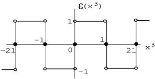
Figure 1: The graph of the periodic sign function $\epsilon({x^{5}})$, (35). Background fields $a_{5}$ and $\varphi$ behave as $a_{5\gamma}({x^{5}})={\bar{a}}_{\gamma}\,\epsilon({x^{5}}){\quad,}\quad\varphi_{\gamma}({x^{5}})={\bar{\varphi}}_{\gamma}\epsilon({x^{5}})$.

It is the thin-wall limit of a (periodic) kink solution and shows the localization of the fields.

The background fields, (35), satisfy the required boundary condition. We show they also satisfy the on-shell condition (12) for an appropriate choice of ${\bar{a}},{\bar{\varphi}},\eta,\eta^{\prime}$ and $\chi^{3}$. The assumed background forms are summarized as

$$\varphi_{\alpha}({x^{5}})={\bar{\varphi}}_{\alpha}\epsilon({x^{5}}){\quad,}\quad a_{5\alpha}({x^{5}})={\bar{a}}_{\alpha}\epsilon({x^{5}}){\quad,}$$

$$\eta_{\alpha^{\prime}}=\mbox{const}{\quad,}\quad\eta^{\prime}_{\alpha^{\prime}}=\mbox{const}{\quad,}\quad d_{\alpha}=\chi^{3}_{\alpha}-\nabla_{5}\varphi_{\alpha}=\mbox{const}{\quad,}$$ (36)

where ”const”’s mean some constants which generally may be different. We note the relation

$$\partial_{5}\varphi_{\gamma}=2{\bar{\varphi}}_{\gamma}\{\delta({x^{5}})-\delta({x^{5}}-l)\}{\quad,}$$ (37)

where $\delta({x^{5}})$ is the periodic delta function with the periodicity $2l$. The above equation expresses the localization of the bulk scalar at ${x^{5}}=0$ and ${x^{5}}=l$. It is considered to be the field theoretical version of the brane-anti-brane configuration. See Fig.2.

Figure 2: Behaviour of $\partial_{5}\varphi_{\gamma}(x^{5})$.

Using this relation, the first two equations of (12) are replaced by

$$\partial_{5}\{-{\bar{\varphi}}_{\alpha}\partial_{5}\epsilon+g\epsilon^{2}({\bar{a}}\times{\bar{\varphi}})_{\alpha}-g(\delta({x^{5}})\eta^{\dagger}T^{\alpha}\eta+\delta({x^{5}}-l)\eta^{\prime{\dagger}}T^{\alpha}\eta^{\prime})\}$$

$$+g\epsilon\{(-{\bar{\varphi}}\partial_{5}\epsilon+g\epsilon^{2}({\bar{a}}\times{\bar{\varphi}})-g(\delta({x^{5}})\eta^{\dagger}T\eta+\delta({x^{5}}-l)\eta^{\prime{\dagger}}T\eta^{\prime}))\times{\bar{a}}\}_{\alpha}=0\ ,$$

$${\bar{a}}_{\alpha}{\partial_{5}}^{2}\epsilon-g\epsilon\{{\bar{\varphi}}\times(-{\bar{\varphi}}\partial_{5}\epsilon+g\epsilon^{2}({\bar{a}}\times{\bar{\varphi}})-g(\delta({x^{5}})\eta^{\dagger}T\eta+\delta({x^{5}}-l)\eta^{\prime{\dagger}}T\eta^{\prime}))\}_{\alpha}=0\ .$$ (38)

We note here the following things.

1. When ${\bar{a}}_{\alpha}\propto{\bar{\varphi}}_{\alpha}$, the following relations hold: $({\bar{a}}\times{\bar{\varphi}})_{\alpha}=f_{{\alpha\beta}\gamma}{\bar{a}}_{\beta}{\bar{\varphi}}_{\gamma}=0$.

2. We may use the equation: $\partial_{5}(\delta({x^{5}})-\delta({x^{5}}-l))\times\mbox{const}=0$, in the field equation on condition that the arbitrary variation $\delta A^{5}_{\alpha}({x^{5}})$, which is used to derive the second equation of (12), satisfies the relation: $\partial_{5}(\delta A^{5}_{\alpha})|_{{x^{5}}=0}=\partial_{5}\delta(\delta A^{5}_{\alpha})|_{{x^{5}}=l}$.

3. $\epsilon({x^{5}})^{2}=1$, $\epsilon({x^{5}})^{3}=\epsilon({x^{5}})$, $\partial_{5}(\epsilon({x^{5}}))=2(\delta({x^{5}})-\delta({x^{5}}-l))$, ${\frac{1}{2}}\partial_{5}\{\epsilon({x^{5}})^{2}\}=(\delta({x^{5}})-\delta({x^{5}}-l))\epsilon({x^{5}})=0$ .

Then we can conclude that (36) is a solution of the field equation (12) for the following choice.

$$\frac{1}{c}{\bar{a}}_{\alpha}={\bar{\varphi}}_{\alpha}=-\frac{g}{2}\eta^{\dagger}T^{\alpha}\eta=\frac{g}{2}\eta^{\prime{\dagger}}T^{\alpha}\eta^{\prime}{\quad,}\quad\chi^{3}_{\alpha}=-g(\delta({x^{5}})-\delta({x^{5}}-l))\eta^{\dagger}T^{\alpha}\eta{\quad,}$$ (39)

where $c$ is a free parameter. In this choice $d_{\alpha}=0$ is concluded. Hence the final two equations of (12) are satisfied. We can regard these as the new on-shell condition due to the restriction of the background fields (35). The present vacuum (minimum point of the effective potential) should be consistent with (39).

(ii) Sawtooth-wave solution

We consider another solution.

$$a_{5\gamma}({x^{5}})={\bar{a}}_{\gamma}\times[{x^{5}}]_{p}{\quad,}\quad\varphi_{\gamma}({x^{5}})={\bar{\varphi}}_{\gamma}\times[{x^{5}}]_{p}{\quad,}$$

$$\mbox{[${x^{5}}$]${}_{p}$}=\left\{\begin{array}[]{cc}{x^{5}}&-l<{x^{5}}<l\\ 0&{x^{5}}=l\\ \mbox{periodic}&\mbox{other regions}\end{array}\right.{\quad,}$$ (43)

where $[{x^{5}}]_{p}$ is the sawtooth-wave (periodic linear function) with the periodicity $2l$. ${\bar{a}}_{\gamma}$ and ${\bar{\varphi}}_{\gamma}$ are some positive constants. See Fig.3.

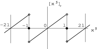
Figure 3: The graph of the sawtooth wave $[{x^{5}}]_{p}$, (43). Background fields $a_{5}$ and $\varphi$ behave as $a_{5\gamma}({x^{5}})={\bar{a}}_{\gamma}\times[{x^{5}}]_{p}{\quad,}\quad\varphi_{\gamma}({x^{5}})={\bar{\varphi}}_{\gamma}\times[{x^{5}}]_{p}$.

Using (43), with the following relations in $-l<{x^{5}}\leq l$: $\partial_{5}\varphi_{\alpha}={\bar{\varphi}}_{\alpha}-2l{\bar{\varphi}}_{\alpha}\delta({x^{5}}-l),{\partial_{5}}^{2}\varphi_{\alpha}=-2l{\bar{\varphi}}_{\alpha}\delta^{\prime}({x^{5}}-l);\partial_{5}a_{5\gamma}={\bar{a}}_{\gamma}-2l{\bar{a}}_{\gamma}\delta({x^{5}}-l),{\partial_{5}}^{2}a_{5\gamma}=-2l{\bar{a}}_{\gamma}\delta^{\prime}({x^{5}}-l)$, we can find a solution in the following way. First we consider, as in the previous solution, the case that the two scalars ${\bar{a}}_{\alpha}$ and ${\bar{\varphi}}_{\alpha}$ are ”parallel” in the isospace:  ${\bar{a}}_{\alpha}=\mbox{const}\times{\bar{\varphi}}_{\alpha}$. Then the key quantity $Z_{\alpha}$ can be written as

$$Z_{\alpha}=d_{\alpha}=-{\bar{\varphi}}_{\alpha}\{1-2l\delta({x^{5}}-l)\}-g\{\delta({x^{5}})\eta^{\dagger}T^{\alpha}\eta+\delta({x^{5}}-l)\eta^{\prime{\dagger}}T^{\alpha}\eta^{\prime}\}{\quad.}$$ (44)

Now we require that $d_{\alpha}$ should be independent of the extra axis ${x^{5}}$. Then we obtain

$$\eta_{\alpha^{\prime}}=\eta^{\dagger}_{\alpha^{\prime}}=0{\quad,}\quad{\bar{\varphi}}_{\alpha}=\frac{g}{2l}\eta^{\prime{\dagger}}T^{\alpha}\eta^{\prime}=\frac{1}{c}{\bar{a}}_{\alpha}{\quad,}\quad Z_{\alpha}=d_{\alpha}=-{\bar{\varphi}}_{\alpha}{\quad,}$$ (45)

where $c$ is a free parameter. The first equation of (12) is satisfied. The second equation requires: ${\bar{a}}_{\alpha}{\partial_{5}}^{2}[{x^{5}}]_{p}=-2l{\bar{a}}_{\alpha}\partial_{5}(\delta({x^{5}}-l))=0$. It means the variation $\delta A_{5\alpha}$, which is used to derive the second equation, should satisfy the Neumann boundary condition:

$$\frac{\partial}{\partial{x^{5}}}\delta A_{5\alpha}|_{{x^{5}}=l}=0{\quad.}$$ (46)

(For a special case $c=0$ ($a_{5\alpha}=0$), the above condition is not necessary.) The third equation gives $\chi^{3}_{\alpha}=-g\delta({x^{5}}-l)\eta^{\prime{\dagger}}T^{\alpha}\eta^{\prime}$. The fourth equation of (12) is satisfied. The fifth equation gives the condition on the values of $\eta^{\prime}_{\alpha^{\prime}}$: 

$$d_{\beta}(T^{\beta}\eta^{\prime})_{\alpha^{\prime}}=-\frac{g}{2l}(\eta^{\prime{\dagger}}T^{\beta}\eta^{\prime})(T^{\beta}\eta^{\prime})_{\alpha^{\prime}}=0{\quad.}$$ (47)

All on-shell conditions are satisfied by the above choice. Especially, $d_{\alpha}=-{\bar{\varphi}}_{\alpha}=-\frac{g}{2l}\eta^{\prime{\dagger}}T^{\alpha}\eta^{\prime}$. From the form of $\partial_{5}\varphi_{\alpha}={\bar{\varphi}}_{\alpha}-2l{\bar{\varphi}}_{\alpha}\delta({x^{5}}-l)$ (see Fig.4), these backgrounds are considered to describe the mixture of a non-localized and a localized (at one end) configurations. The form of the sawtooth-wave solution (Fig.3) is reminiscent of the AdS₅ solution of the dilaton in the Randall-Sundrum model although the latter one is Z₂ even whereas the present one is Z₂ odd.

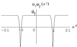
Figure 4: Behaviour of $\partial_{5}\varphi_{\gamma}(x^{5})$ for the sawtooth wave solution (43).

Taking the localized solution (i), we evaluate $S^{(2)}$, (31), furthermore. From the periodicity (${x^{5}}\rightarrow{x^{5}}+2l$) and the Z₂ property, the bulk quantum fields $\Phi(X),A_{5}(X)$ and $c(X)$ can be KK-expanded as

$$\Phi(x,{x^{5}})=\frac{1}{\sqrt{l}}\sum_{n=1}^{\infty}\Phi_{n}(x)\sin({\frac{n\pi}{l}}{x^{5}}){\quad,}\quad A_{5}(x,{x^{5}})=\frac{1}{\sqrt{l}}\sum_{n=1}^{\infty}A_{n}(x)\sin({\frac{n\pi}{l}}{x^{5}}){\quad,}$$

$$c(x,{x^{5}})=\frac{1}{2\sqrt{l}}\left\{c_{0}(x)+2\sum_{n=1}^{\infty}c_{n}(x)\cos({\frac{n\pi}{l}}{x^{5}})\right\}{\quad.}$$ (48)

(The $Z_{2}$-parity of the ghost field is even because it should be the same as that of the gauge parameter $\Lambda$ : $\delta A^{M}=\partial^{M}\Lambda-ig[A^{M},\Lambda]$. ) Now we use the Fourier expansion of the periodic sign function,

$$\epsilon(x)=\frac{4}{\pi}\sum_{n=0}^{\infty}\frac{1}{2n+1}\sin\{\frac{(2n+1)\pi}{l}x\}{\quad,}$$ (49)

and the relation:

$$\int_{-l}^{l}d{x^{5}}\epsilon({x^{5}})\cos({\frac{m\pi}{l}}{x^{5}})\sin({\frac{n\pi}{l}}{x^{5}})=-\frac{2l}{\pi}Q_{mn}{\quad,}$$

$$Q_{mn}=\left\{\begin{array}[]{cc}\frac{1}{m-n}&m-n=\mbox{odd}\\ 0&m-n=\mbox{even}\end{array}\right.{\quad.}$$ (52)

Noting the above equations and (37), we can express $S^{(2)}$ in terms of the 4D integral as follows.

$$S^{(2)}=S^{ghost}+\int d^{4}x\times$$

$${\frac{1}{2}}\left(\begin{array}[]{cccc}\phi^{\dagger}_{\alpha^{\prime}}&\phi_{\alpha^{\prime}}&\Phi_{m\alpha}&A_{m\alpha}\end{array}\right){\left(\begin{array}[]{cc}\left(\begin{array}[]{cc}{\cal M}_{\phi^{\dagger}\phi}&{\cal M}_{\phi^{\dagger}\phi^{\dagger}}\\ {\cal M}_{\phi\phi}&{\cal M}_{\phi\phi^{\dagger}}\\ \end{array}\right)_{{\alpha^{\prime}}\,{\beta^{\prime}}}&\left(\begin{array}[]{cc}{\cal M}_{\phi^{\dagger}\Phi}&0\\ {\cal M}_{\phi\Phi}&0\end{array}\right)_{{\alpha^{\prime}}\,n\beta}\\ \left(\begin{array}[]{cc}{\cal M}_{\Phi\phi}&{\cal M}_{\Phi\phi^{\dagger}}\\ 0&0\end{array}\right)_{m\alpha\,{\beta^{\prime}}}&\left(\begin{array}[]{cc}{\cal M}_{\Phi\Phi}&{\cal M}_{\Phi A}\\ {\cal M}_{A\Phi}&{\cal M}_{AA}\end{array}\right)_{m\alpha\,n\beta}\end{array}\right)}\left(\begin{array}[]{c}\phi_{\beta^{\prime}}\\ \phi^{\dagger}_{\beta^{\prime}}\\ \Phi_{n\beta}\\ A_{n\beta}\end{array}\right),$$ (68)

where the integer suffixes $m$ and $n$ runs from 1 to $\infty$, and each component is described as

$${\cal M}_{\phi^{\dagger}_{\alpha^{\prime}}\phi_{\beta^{\prime}}}=\partial^{2}\delta_{{\alpha^{\prime}}{\beta^{\prime}}}+gd_{\gamma}(T^{\gamma})_{{\alpha^{\prime}}{\beta^{\prime}}}-g^{2}\delta(0)(T^{\gamma}\eta)_{\alpha^{\prime}}(\eta^{\dagger}T^{\gamma})_{\beta^{\prime}}{\quad,}$$

$${\cal M}_{\phi^{\dagger}_{\alpha^{\prime}}\phi^{\dagger}_{\beta^{\prime}}}=-g^{2}\delta(0)(T^{\gamma}\eta)_{\alpha^{\prime}}(T^{\gamma}\eta)_{\beta^{\prime}}{\quad,}\quad{\cal M}_{\phi_{\alpha^{\prime}}\phi_{\beta^{\prime}}}=-g^{2}\delta(0)(\eta^{\dagger}T^{\gamma})_{\alpha^{\prime}}(\eta^{\dagger}T^{\gamma})_{\beta^{\prime}}{\quad,}$$

$${\cal M}_{\phi_{\alpha^{\prime}}\phi^{\dagger}_{\beta^{\prime}}}=\partial^{2}\delta_{{\alpha^{\prime}}{\beta^{\prime}}}+gd_{\gamma}(T^{\gamma})_{{\beta^{\prime}}{\alpha^{\prime}}}-g^{2}\delta(0)(\eta^{\dagger}T^{\gamma})_{\alpha^{\prime}}(T^{\gamma}\eta)_{\beta^{\prime}}{\quad,}$$

$${\cal M}_{\phi^{\dagger}_{\alpha^{\prime}}\Phi_{n\beta}}=-\frac{g}{\sqrt{l}}(T^{\beta}\eta)_{\alpha^{\prime}}{\frac{n\pi}{l}}={\cal M}_{\Phi_{n\beta}\phi^{\dagger}_{\alpha^{\prime}}}{\quad,}\quad{\cal M}_{\phi_{\alpha^{\prime}}\Phi_{n\beta}}=-\frac{g}{\sqrt{l}}(\eta^{\dagger}T^{\beta})_{\alpha^{\prime}}{\frac{n\pi}{l}}={\cal M}_{\Phi_{n\beta}\phi_{\alpha^{\prime}}}{\quad,}$$

$${\cal M}_{\Phi_{m\alpha}\Phi_{n\beta}}=-\{-\partial^{2}+({\frac{n\pi}{l}})^{2}\}\delta_{mn}\delta_{\alpha\beta}-g^{2}f_{\alpha\delta\tau}f_{\beta\gamma\tau}{\bar{a}}_{\delta}{\bar{a}}_{\gamma}\delta_{mn}+\frac{4g}{l}f_{{\alpha\beta}\gamma}{\bar{a}}_{\gamma}mQ_{mn}{\quad,}$$

$${\cal M}_{\Phi_{m\alpha}A_{n\beta}}=g^{2}f_{{\alpha\beta}\tau}f_{\gamma\delta\tau}{\bar{a}}_{\gamma}{\bar{\varphi}}_{\delta}\delta_{mn}-g^{2}f_{\gamma\alpha\tau}f_{\beta\delta\tau}{\bar{a}}_{\gamma}{\bar{\varphi}}_{\delta}\delta_{mn}-\frac{2g}{l}f_{{\alpha\beta}\gamma}{\bar{\varphi}}_{\gamma}mQ_{mn}={\cal M}_{A_{n\beta}\Phi_{m\alpha}},$$

$${\cal M}_{A_{m\alpha}A_{n\beta}}=-\{-\partial^{2}+({\frac{n\pi}{l}})^{2}\}\delta_{mn}\delta_{\alpha\beta}-g^{2}f_{\alpha\gamma\tau}f_{\beta\delta\tau}{\bar{\varphi}}_{\gamma}{\bar{\varphi}}_{\delta}\delta_{mn}{\quad,}$$ (69)

where the kinetic (free) part is also included ($\partial^{2}\equiv\partial_{m}\partial^{m}$) in the “Mass” matrix and the repeated indices imply the Einstein’s summation convention. $S^{ghost}$ is decoupled and is given by

$$S^{ghost}=\int d^{4}x\left\{{\frac{1}{2}}\partial_{m}{\bar{c}}_{0\alpha}\partial^{m}c_{0\alpha}+\sum_{k=1}^{\infty}\left(\partial_{m}{\bar{c}}_{k\alpha}\partial^{m}c_{k\alpha}-(\frac{k\pi}{l})^{2}{\bar{c}}_{k\alpha}c_{k\alpha}\right)\right.$$

$$+\left.\sum_{n=1}^{\infty}\sum_{k=1}^{\infty}{\bar{c}}_{n\alpha}(x)[-\frac{2ig}{l}f_{\alpha\gamma\beta}{\bar{a}}_{\gamma}nQ_{nk}]c_{k\beta}(x)\right\}{\quad.}$$ (70)

This contribution is treated independently from others.

5 Effective Potential of Bulk-Boundary System The effective potential is obtained from the eigen values of the mass-matrix obtained in (68),(69) and (70). We examine the behaviour for two typical cases.

(A)$\eta=0,\eta^{\dagger}=0$(Bulk-Boundary decoupled case)
We look at the potential from the vanishing scalar-matter point. In this case the singular terms, $\delta(0)$-terms, disappear and the matrix ${\cal M}$ decouples to the boundary part ($\phi,\phi^{\dagger}$) and the bulk part ($\Phi,A$). The former part gives the following eigen values.

$$\lambda_{\pm}=-k^{2}\pm\frac{g}{2}\sqrt{d^{2}}{\quad,}\quad d^{2}\equiv{d_{1}}^{2}+{d_{2}}^{2}+{d_{3}}^{2}{\quad,}\quad k^{2}=k_{m}k^{m}{\quad,}$$ (71)

where we take G=SU(2) and the doublet representation for the boundary matter fields. $k^{m}$ is the 4D momentum. This gives, taking the supersymmetric boundary condition, the following potential before the renormalization:

$$V^{eff}_{1-loop}=\int\frac{d^{4}k}{(2\pi)^{4}}\ln\{1-\frac{g^{2}}{4}\frac{d^{2}}{(k^{2})^{2}}\}=-\frac{g^{2}}{4}\int\frac{d^{4}k}{(2\pi)^{4}}\frac{d^{2}}{(k^{2})^{2}}+O(g^{4}){\quad,}$$ (72)

The last perturbative (w.r.t. $g$ ) form is logarithmically divergent. It can be checked by the perturbative calculation. It is renormalized by the bulk wave function of $X^{3}$ and $\Phi$. Here the 4D world’s connection to the Bulk world appears. The quantum fluctuation within the boundary influence the bulk world through the renormalization. The form of (72) is similar to the 4D super QED[7]. We see the present model produces a desired effective potential on the brane.

The bulk part of ${\cal M}$ and the ghost part do not depend on the field $d$. They and their eigenvalues depend only on the brane parameters, ${\bar{a}}$ and ${\bar{\varphi}}$, and the size of the extra space, $l$. In the SUSY boundary condition, their contribution to the vacuum energy is zero. The scalar loop contribution is expected to be cancelled by the quantum effect of the non-scalar fields. Let us, however, examine the scalar-loop contribution to the Casimir energy (potential). General case is technically difficult. We consider the large circle limit: ${\hat{g}}^{2}\equiv\frac{g^{2}}{l}=\mbox{fixed}\ll 1\ ,\ {\hat{a}}=\sqrt{l}{\bar{a}}=\mbox{fixed}\ ,\ {\hat{\varphi}}=\sqrt{l}{\bar{\varphi}}=\mbox{fixed}\ ,\ l\rightarrow\infty$. This is the situation where the circle is large compared with the inverse of the domain wall height. (${\hat{a}}$ and ${\hat{\varphi}}$ have the dimension of $M$. ) We notice, in this limit, $Q_{mn}$-terms disappear. In the ”propagator” terms of the bulk quantum fields, KK-mass terms $m^{2}\pi^{2}/l^{2}$ disappear. All KK-modes equally contribute to the vaccum energy. The eigen values of the bulk part of ${\cal M}$ can be easily obtained. In particular, for the special case ${\hat{a}}=0$, the nontrivial factor is only $k^{2}+{\hat{g}}^{2}{\hat{\varphi}}^{2}$. Hence each KK-mode equally contributes to the vacuum energy as

$$V^{eff}_{1KK-mode}\propto\int\frac{d^{4}k}{(2\pi)^{4}}\ln\{1+{\hat{g}}^{2}\frac{{\hat{\varphi}}^{2}}{k^{2}}\}{\quad,}$$ (73)

This quantity is quadratically divergent. After an appropriate normalization, the final form should become, based on the dimensional analysis, the following one.

$$V^{eff}_{1-loop}={\hat{g}}^{2}(c_{1}\frac{{\hat{\varphi}}^{2}}{l^{2}}+c_{2}\frac{{\hat{a}}^{2}}{l^{2}}+c_{3}\frac{{\hat{a}}\cdot{\hat{\varphi}}}{l^{2}})+O({\hat{g}}^{4}){\quad,}$$ (74)

where $c_{1},c_{2}$ and $c_{3}$ are some finite constants which are calculable after we know the bulk quantum dynamics sufficiently. This is a new type Casimir energy. This is the reason why we have examined the scalar-loop contribution. Comparing the ordinary one (76) explained soon, it is new in the following points: 1) it depends on the brane parameters ${\hat{\varphi}}$ and ${\hat{a}}$ besides the extra-space size $l$; 2) it depends on the gauge coupling ${\hat{g}}$; 3) it is proportional to $1/l^{2}$.

We expect the above result of Casimir energy are cancelled by the spinor and vector-loop contribution in the present SUSY theory. The unstable Casimir potential do not appear in SUSY theory.

(B)${\bar{a}}=0,{\bar{\varphi}}=0$
In this case, $Q_{mn}$-terms disappear and we do have no localized (brane) configuration. The bulk background configuration is trivial: $a_{5}({x^{5}})=0,\ \varphi({x^{5}})=0$. 5D bulk quantum fields fluctuate with the periodic boundary condition in the extra space. This is similar to the 5D Kaluza-Klein case mentioned in the introduction. The eigen values for the bulk part, $c(X),{\bar{c}}(X),\Phi(X)$ and $A_{5}(X)$ are commonly given by,

$$\lambda_{n}=-k^{2}-({\frac{n\pi}{l}})^{2}{\quad,}\quad n=1,2,3,\cdots{\quad,}$$ (75)

The eigen values are basically the same as the KK case [3]. They depend only on the radius (or the periodicity) parameter $l$. It gives the scalar-loop contribution to the Casimir potential. From the dimensional analysis, after the renormalization, it has the following form.

$$\frac{1}{l}V^{eff}_{scalar}=\frac{\mbox{const}}{l^{5}}{\quad.}$$ (76)

We expect again this contribution is cancelled by the spinor and vector fields.

The eigenvalues for the boundary part is obtained as a complicated expression involving the following terms:

$$S\equiv\eta^{\dagger}\eta\ ,\ d^{2}=d_{\alpha}d_{\alpha}\ ,\ d\cdot V\equiv d_{\alpha}\,\eta^{\dagger}T^{\alpha}\eta\ ,\ V^{2}\equiv(\eta^{\dagger}T^{\alpha}\eta)^{2}{\quad.}$$ (77)

We have the full expression in the computer file. In the manipulation of eigen-values search (determinant calculation), we face the following combination of terms.

$$\delta(0)+\frac{1}{l}\sum_{m=1}^{\infty}\frac{(\pi m/l)^{2}}{-\lambda-k^{2}-(\pi m/l)^{2}}{\quad.}$$ (78)

The first term comes from the singular terms in ${\cal M}$, the second from the KK-mode sum. Using the relation$\sum_{m\in{\bf Z}}1=2l\delta(0)$, the above sum leads to a regular quantity.

$${\delta(0)}|_{sm}=\frac{1}{2l}\sum_{m\in{\bf Z}}\frac{\lambda+k^{2}}{\lambda+k^{2}+(\pi m/l)^{2}}=\left\{\begin{array}[]{cc}{\frac{1}{2}}\sqrt{\lambda+k^{2}}\coth\{l\sqrt{\lambda+k^{2}}\}&\lambda>-k^{2}\\ {\frac{1}{2}}\sqrt{-\lambda-k^{2}}\cot\{l\sqrt{-\lambda-k^{2}}\}&-k^{2}>\lambda\end{array}\right.{\quad.}$$ (81)

We have confirmed this ”smoothing” phenomenon occurs at the 1-loop full level.

For some interesting cases, we present the explicit forms of the eigenvalues.
(i) $\eta=\eta^{\dagger}=0\ (d\cdot V=0,V^{2}=0,S=0)$
This is a special case of (A), the decoupled case.

$$\lambda_{1}=\lambda_{2}=\lambda_{+}{\quad,}\quad\lambda_{3}=\lambda_{4}=\lambda_{-}{\quad,}\quad\lambda_{\pm}=-k^{2}\pm\frac{g}{2}\sqrt{d^{2}}{\quad.}$$ (82)

It is consistent with Case (A).

(ii) $d\cdot V\neq 0$, others=$0$ ($S=0,d^{2}=0,V^{2}=0$)
Interesting eigenvalues come from the solutions of the following equation.

$$\quad(\lambda+k^{2})^{2}-\frac{g^{3}}{2}d\cdot V\frac{\sqrt{\lambda+k^{2}}}{2}\coth l\sqrt{\lambda+k^{2}}=0{\quad.}$$ (83)

To confirm the correctness, we look at the perturbative aspect of this 1-loop full result. First expanding the above expression by $1/k^{2}$ (propagator expansion), and then taking the terms up to the 1st order w.r.t. $g^{2}/l$, we obtain

$$(\lambda+k^{2})^{2}-\frac{g^{3}}{4}d\cdot V\sqrt{k^{2}}\coth l\sqrt{k^{2}}=0{\quad.}$$ (84)

Two eigenvalues $\lambda_{1},\lambda_{2}$ satisfy

$$\lambda_{1}\lambda_{2}=(k^{2})^{2}\left(1-\frac{g^{3}}{4}d\cdot V\frac{\sqrt{k^{2}}\coth l\sqrt{k^{2}}}{(k^{2})^{2}}\right){\quad.}$$ (85)

This result is consistent with the perturbative result (the vertex correction on the boundary) up to the order of $g^{3}$. The full-order eigenvalues, the solutions of (83), correspond to the 1-loop full effective potential.

6 Conclusion We have analyzed the effective potential of the Mirabelli-Peskin model. The explicit forms are obtained for some cases. An interesting localized configuration (solution) is found in the bulk scalar and the extra-component of the bulk vector when we solve the field equation (on-shell condition). The vacuum is generalized in connection with the treatment of the extra axis. We treat ${x^{5}}$ as a parameter which is independent of the 4D world. The important role of the D-field, ${\cal D}_{\alpha}=X^{3}_{\alpha}-\nabla_{5}(A)\Phi_{\alpha}$, in the 4D world is confirmed. In this SUSY invariant theory, the Casimir force vanishes. Its scalar-loop contribution is obtained from the explicit matrix elements depending on the boundary parameters ${\bar{a}}$, ${\bar{\varphi}}$ and $l$. Besides the ordinary type, we find a new type form of the Casimir energy which is characteristic for the brane model. When SUSY is broken in some mechanism, the new type potential could become an important distinguished quantity of the bulk-boundary system from the ordinary KK system.

We hope the present result improves the understanding of the quantum dynamics of the bulk-boundary system.

The authors thank N. Sakai for valuable comments when this work, still at the primitive stage, was presented at the Chubu Summer School 2002 (Tsumagoi, Gunma, Japan, 2002.8.30-9.2). A part of this work was done when one of the author (S.I.) stayed at DAMTP(Univ. of Cambridge,2002.11.22-2003.2.10). He thanks G.W. Gibbons and G. Silva for comments and discussions. The hospitality there is acknowledged. He also thanks the governor of the Shizuoka prefecture for the financial support.

References

[1] P.Hořava and E.Witten,
Nucl.Phys.B460(1996)506,hep-th/9510209
[2] E.A.Mirabelli and M.E. Peskin,
Phys.Rev.D58(1998)065002, hep-th/9712214
[3] T. Appelquist and A. Chodos, Phys.Rev.D28(1983)772; Phys.Rev.Lett.50(1983)141
[4] S. Ichinose, Phys.Lett.152B(1985)56
[5] A. Hebecker, Nucl.Phys.B632(2002)101
[6] R. D.C. Miller, Phys.Lett.124B(1983)59
[7] R. D.C. Miller,Nucl.Phys.B229(1983)189
[8] S.Weinberg, Phys.Rev.D7(1973)2887
[9] A. Murayama, Int.Jour.Mod.Phys.A13(1998)4257
[10] B.S. DeWitt, Phys.Rev.162(1967)1195,1239
[11] G.’t Hooft, Nucl.Phys.B62(1973)444
[12] S. Ichinose and M. Omote, Nucl.Phys.B203(1982)221