We show that many numerically established properties of Q-balls can be understood in terms of analytic approximations for a certain type of potential. In particular, we derive an explicit formula between the energy and the charge of the Q-ball valid for a wide range of the charge $Q$ .

1 Introduction

As shown by Coleman [1], the existence of Q-balls is a general feature of scalar field theories carrying a conserved $U(1)$ charge [2]. Q-balls can be understood as bound states of scalar particles and appear as stable classical solutions (nontopological solitons) carrying a rotating time dependent internal phase. They are characterized by a conserved nontopological charge $Q$ (Noether charge) which is responsible for their stability (see, for example, Refs. [3]-[4]). These features differentiate the Q-ball interaction properties from those of the topological solitons since here the charge $Q$ can take arbitrary values in a specific range, allowing for the possibility of charge transfer between solitons during the interaction process.

The concepts associated with Q-balls are extremely general and occur in a wide variety of physical contexts [5]. Q-balls are a generic consequence of the Minimal Supersymmetric Standard Model (MSSM) [6] where leptonic and baryonic balls may exist. In this context the conserved charge is associated with the $U(1)$ symmetries leading to baryon and lepton number conservation, and the relevant $U(1)$ fields correspond to either squark or slepton particles. Thus, the Q-balls can be thought of as condensates of either squark or slepton particles. It has been suggested that such condensates can affect baryogenesis via the Affleck-Dine mechanism [7] during the post-inflationary period of the early universe. Then, two interesting possibilities occur: (i) If the Q-balls are stable and avoid evaporation into lighter stable particles like protons, they are cosmologically important since they can contribute to the dark matter content of the universe [8]; (ii) If they are unstable, they decay in a nontrivial way into baryons protecting them from erasure through sphaleron transitions [9].

Up till now, comprehensive studies of these objects have been made by using either numerical simulations [3]-[11] or some analytic considerations [1, 12, 13]. In our approach we will semi-analytically identify the explicit relation between the energy and the charge of the Q-balls by using a semi-Bogomolny argument in the energy density. Subsequently, we will show that similar results can be obtained by using the Woods-Saxon ansatz for describing the Q-ball profile function; an approach which has been successfully applied to describe analytically the properties of multi-skyrmions in three [14] and two spatial dimensions [15]. This way, some universal properties of Q-balls in the thin-wall limit can be established.

2 Energy of the Q-balls

Although Q-balls can exist in a variety of field theoretical models, we will consider the $U(1)$ Goldstone model describing a single complex scalar field $\phi$ in three spatial dimensions with potential $U(|\phi|)$. The Lagrangian is

$${\cal L}=\frac{1}{2}\partial_{\mu}\phi\,\partial^{\mu}\bar{\phi}-U(|\phi|)$$ (1)

where the potential is only a function of $|\phi|$ and has a single minimum at $\phi=0$. This is equivalent of stating that there is a sector scalar particles (mesons) carrying $U(1)$ charge and having mass squared equal to $\frac{1}{2}U^{\prime\prime}(0)$. The corresponding energy functional is given by

$$E=\int\left(\frac{1}{2}|\partial_{t}{\phi}|^{2}+\frac{1}{2}|\nabla\phi|^{2}+U(|\phi|)\right)d^{3}x.$$ (2)

The model has a global $U(1)$ symmetry leading to the conserved Noether current

$$J_{\mu}=\frac{1}{2i}\left(\bar{\phi}\,\partial_{\mu}\phi-\phi\,\partial_{\mu}\bar{\phi}\right).$$ (3)

The conserved Noether charge $Q$ is

$$Q=\frac{1}{2i}\int\left(\bar{\phi}\,\partial_{t}\phi-\phi\,\partial_{t}\bar{\phi}\right)d^{3}x.$$ (4)

A stationary Q-ball solution has the form

$$\phi=e^{i\omega t}f(r)$$ (5)

where $f(r)$ is a real radial profile function which satisfies the ordinary differential equation

$$\frac{d^{2}f}{dr^{2}}=-\frac{2}{r}\frac{df}{dr}-\omega^{2}f+U^{\prime}(f)$$ (6)

with boundary conditions $f(\infty)=0$ and $f^{\prime}(0)=0$.

This equation can either be interpreted as describing the motion of a point particle moving in a potential with friction [1], or in terms of Euclidean bounce solutions [16]. In each case the effective potential being $U_{eff}(f)=\omega^{2}f^{2}/2-U(f)$ leads to constraints on the potential $U(f)$ and the frequency $\omega$ in order for a Q-ball solution to exist. Firstly, the effective mass of $f$ must be negative. If we consider a potential $U(f)$ which is non-negative and satisfies $U(0)=U^{\prime}(0)=0$, $U^{\prime\prime}(0)=\omega_{+}^{2}>0$ then one can deduce that $\omega<\omega_{+}$. Furthermore, the minimum of $U(f)/f^{2}$ must be attained at some positive value of $f$, say $0<f_{0}<\infty$ and existence of the solution requires that $\omega>\omega_{-}$ where $\omega_{-}^{2}=2U(f_{0})/f_{0}^{2}$. Hence, Q-balls exist for all $\omega$ in the range $\omega_{-}<|\omega|<\omega_{+}$.

Thus, the charge $Q$ of a stationary Q-ball solution simplifies to

$$Q \doteq \omega I[f]$$ (7)

$$= 4\pi\omega\int r^{2}f^{2}(r)\,dr$$

where $I[f]$ is the moment of inertia. Numerical and analytical methods have shown that when the internal frequency is close to the minimal value $\omega_{-}$, the profile function is almost constant, implying that the charge (7) is large (thin-wall approximation). On the other hand, when the internal frequency approaches the maximal value $\omega_{+}$ the profile function falls off very quickly (thick-wall approximation). In the thick-wall approximation the behavior of the charge $Q$ depends on the particular form of the potential and the number of dimensions [13]. In the case studied here we show that $Q\rightarrow\infty$ as $\omega\rightarrow\omega_{+}$.

In order to derive the minimum of the energy of the Q-ball at fixed charge $Q$, it is convenient to represent the energy in the form

$$E_{{}_{{\tiny Q}}}=\frac{Q^{2}}{2I[f]}\,+4\pi\int\left(\frac{f^{\prime}{}^{2}}{2}+U(f)\right)r^{2}\,dr$$ (8)

where the stabilizing role of the Q-ball rotational part is obvious. Note that, without rotational energy the Q-ball would collapse since $E_{{}_{Q}}\rightarrow 0$ as $f(r)\rightarrow 0$ everywhere except at the origin $r=0$. This is similar to the case of rotating skyrmions when the 4-th order Skyrme term is omitted in the Lagrangian. The zero mode (rotational) quantum correction to the energy, which is proportional to $(I[f])^{-1}$ plays a stabilizing role in this case.

The choice of the potential is not unique, the standard requirement is that the function $U(f)/f^{2}$ has a local minimum at some value of $f$ different from zero. Here we will consider the following potential

$$U(f)=f^{2}\left[1+(1-f^{2})^{2}\right].$$ (9)

Note that $\omega_{+}=2$ and $\omega_{-}=\sqrt{2}$ and so that stable Q-balls exist for $\sqrt{2}<\omega<2$.

3 Semi-Bogomolny Argument

We now proceed to obtain an ansatz for the profile function by applying a semi-Bogomolny argument [17] in the energy functional (8-9). Initially, this approach was applied to the Skyrme model [18], where it was shown that the lower energy bound is proportional to the topological charge. Although the model studied here is not a topological one (ie there is no topological charge), the Bogomolny argument can still be applied and leads to an upper energy bound. This way, the profile function satisfies an exactly soluble first order differential equation and the corresponding energy and charge density can be easily derived. The same approach was applied for description of multi-skyrmions properties, as presented in [14, 15].

The energy (8-9) using the Bogomolny argument can be expressed as:

$$E_{{}_{B}} = \left(\frac{\omega}{2}+\frac{1}{\omega}\right)Q+4\pi\int\left(\frac{1}{2}\left(f^{\prime}\right)^{2}+f^{2}\left(1-f^{2}\right)^{2}\right)r^{2}dr$$ (10)

$$= \left(\frac{\omega}{2}+\frac{1}{\omega}\right)Q+4\pi\int\left(\frac{f^{\prime}}{\sqrt{2}}+f\left(1-f^{2}\right)\right)^{2}r^{2}\,dr-4\pi\int\sqrt{2}f^{\prime}f\left(1-f^{2}\right)r^{2}\,dr$$

$$\geq \left(\frac{\omega}{2}+\frac{1}{\omega}\right)Q-4\pi\int\sqrt{2}f^{\prime}f\left(1-f^{2}\right)r^{2}\,dr.$$

The equality is satisfied when the total square term is zero which gives the semi-Bogomolny equation

$$f^{\prime}=-\sqrt{2}f(1-f^{2})\,.$$ (11)

The corresponding profile function has the simple form

$$f(r)=\frac{1}{\sqrt{1+C_{{}_{B}}\,\exp\left(2\sqrt{2}\,r\right)}},\hskip 14.22636ptC_{{}_{B}}>0$$ (12)

which satisfies the boundary conditions $f(0)=1/\sqrt{1+C_{{}_{B}}}$ and $f(\infty)=0$, while $f^{\prime}(0)=-\sqrt{2}C_{{}_{B}}/(1+C_{{}_{B}})^{3/2}$. Note that the asymptotic value of (12): $f\sim\exp(-\sqrt{2}r)$ is in agreement with the equation of motion (6) for $\omega=\sqrt{2}$ (ie for large values of $Q$). In fact, inside the $Q$-ball $f^{\prime}\sim 0$ and $f\sim 1$, while outside the $Q$-ball $f^{\prime}=\,0$ and $f=0$ and so (12) describes accurately the profile function of the Q-ball outside and inside its region where the last term in (10) vanishes. However, (12) does not describe accurately the profile function of the $Q$-ball on its surface (the so-called transition region). Although, in the thin-wall approximation the analytical and numerical results (presented in Table 1) converge as $Q$ increases since the relative contribution of the surface decreases like $Q^{-1/3}$ at large $Q$.

For the specific form of the profile function (12) the charge and the energy can be evaluated explicitly. We find that

$$Q_{{}_{B}} \simeq -\frac{\pi\omega}{2\sqrt{2}}\left(\frac{\pi^{2}}{6}\,\ln\left(C_{{}_{B}}\right)+\frac{1}{6}\,[\ln\left(C_{{}_{B}}\right)]^{3}+Li_{3}\left[-C_{{}_{B}}\right]\right),$$

$$E_{{}_{B}} \simeq \left(\frac{\omega}{2}+\frac{1}{\omega}\right)Q+\frac{\sqrt{2}\pi}{4}\left(\frac{\pi^{2}}{6}+\frac{1}{2}\left[\ln(C_{{}_{B}})\right]^{2}+\ln\left(1+\frac{1}{C_{{}_{B}}}\right)+Li_{2}\left[-C_{{}_{B}}\right]\right)$$ (13)

where $Li_{n}(z)=\int_{0}^{z}\frac{Li_{n-1}(y)}{{y}}\,dy$ and $Li_{1}(y)=\ln(1-y)$ is the polylogarithm function.

Next, the equation for the energy $E_{{}_{B}}$ above has to be minimized with respect to $C_{{}_{B}}$ while $Q_{{}_{B}}$ is kept constant. We expect the semi-Bogomolny ansatz to be valid only when $C_{{}_{B}}\approx 0$ where the initial “velocity” of the trial profile function $f(r)$ tends to zero. In this region, the logarithms will dominate the dilogarithm and the trilogarithm functions respectively, since these functions tend to zero like polynomials. Thus, by substituting $z=-\ln(C_{{}_{B}})$ for $z>0$ one obtains

$$Q_{{}_{B}} = \frac{\pi\omega z}{12\sqrt{2}}\left(\pi^{2}+z^{2}\right),$$

$$E_{{}_{B}} = \left(\frac{\omega}{2}+\frac{1}{\omega}\right)Q_{{}_{B}}+\frac{\sqrt{2}\pi}{4}\left(\frac{\pi^{2}+3z^{2}}{6}+z\right).$$ (14)

One can explicitly solve $\omega$ in terms of the charge $Q_{{}_{B}}$ given above in order to obtain that

$$\omega=\frac{12\sqrt{2}\,Q_{{}_{B}}}{\pi z\left(\pi^{2}+z^{2}\right)}$$ (15)

which when substituted into the energy gives

$$E_{{}_{B}}=\frac{6\sqrt{2}\,Q_{{}_{B}}^{2}}{\pi z\left(\pi^{2}+z^{2}\right)}+\frac{\pi z\left(\pi^{2}+z^{2}\right)}{12\sqrt{2}}+\frac{\sqrt{2}\pi}{4}\left(\frac{\pi^{2}+3z^{2}}{6}+z\right).$$ (16)

Now, upon minimizing the energy with respect to $z$ we find that the frequency $\omega$ and the charge $Q_{{}_{B}}$ are given by

$$\omega^{2} = 2+\frac{12\,\left(1+z\right)}{\pi^{2}+3z^{2}},$$

$$Q_{{}_{B}}^{2} = \frac{\pi^{2}z^{2}\left(\pi^{2}+z^{2}\right)^{2}}{144\left(\pi^{2}+3z^{2}\right)}\left(6+6z+\pi^{2}+3z^{2}\right).$$ (17)

Finally, the relation between $z$ and $\omega$ is

$$z=\frac{2}{\left(\omega^{2}-2\right)}\left(1+\sqrt{1-\frac{\pi^{2}}{12}\left(\omega^{2}-2\right)^{2}+\left(\omega^{2}-2\right)}\,\right).$$ (18)

It is obvious that in the limit $\omega\rightarrow\sqrt{2}$ the parameter $z$ goes to infinity in consistency with the analytical results (14). Thus, the semi-Bogomolny argument is valid in the thin-wall approximation.

The elimination of the $z$ variable from the equations that define $Q_{{}_{B}}$ and $\omega$ can be easily performed. By letting $\varepsilon=\omega^{2}-2$ one gets

$$z = \frac{2}{\varepsilon}\left(1+\sqrt{1+\varepsilon-\frac{\pi^{2}}{12}\,\varepsilon^{2}}\,\right),$$ (19)

$$Q_{{}_{B}} = \frac{\pi\sqrt{2+\varepsilon}\left(24+18\varepsilon+\left[24+\varepsilon\left(6+\pi^{2}\varepsilon\right)\right]\sqrt{1+\varepsilon-\frac{\pi^{2}}{12}~{}\varepsilon^{2}}\,\right)}{9\sqrt{2}\varepsilon^{3}},$$ (20)

$$E_{{}_{B}} = \frac{\pi\left(2+\varepsilon\right)}{\sqrt{2}\,\varepsilon^{2}}\sqrt{1+\varepsilon-\frac{\pi^{2}}{12}~{}\varepsilon^{2}}+\frac{\pi\sqrt{2}\left(1+\varepsilon\right)}{\varepsilon^{2}}+\frac{4+\varepsilon}{2\sqrt{2+\varepsilon}}\,Q_{{}_{B}}\ \cdot$$ (21)

It is obvious that $Q_{{}_{B}}\rightarrow\infty$ as $\omega\rightarrow\sqrt{2}$ (which corresponds to $\varepsilon\rightarrow 0$) while the upper energy limit for any value of $Q$ (or $\varepsilon$) can be obtained from (21).

Next, by eliminating $\varepsilon$ between $Q_{{}_{B}}$ and $E_{{}_{B}}$ we get the Q-ball energy-charge dependence since

$$E_{{}_{B}}\!\!\!\! = \!\!\!\!\sqrt{2}\,Q_{{}_{B}}+\frac{3^{2/3}\pi^{1/3}}{2^{7/6}}\,Q_{{}_{B}}^{2/3}+\frac{5\pi^{2/3}}{2^{11/6}3^{2/3}}\,Q_{{}_{B}}^{1/3}-\frac{\pi\left(4+3\pi^{2}\right)}{36\sqrt{2}}+\frac{\pi^{4/3}\left(17-216\pi^{2}\right)}{2592~{}2^{1/6}~{}3^{1/3}}\ Q_{{}_{B}}^{-1/3}$$ (22)

$$\!\!\!\!+\frac{\pi^{5/3}\left(20-54\pi^{2}+27\pi^{4}\right)}{1944~{}2^{5/6}~{}3^{2/3}}\,Q_{{}_{B}}^{-2/3}+O\left(Q_{{}_{B}}^{-1}\right).$$

Note that for large values of $Q$ (ie for $Q^{1/3}\gg 1$) the expression (22) gives the upper energy bound. In Table 1 we compare the results obtained from the semi-Bogomolny argument by means of (22) with the ones obtained by solving the full second order differential equations (6) numerically, for different values of $Q$. The agreement is impressive and appears to extend far beyond the expected range of validity of the semi-Bogomolny argument.

$Q$	$E_{{}_{num}}$	$E_{{}_{B}}$	$\omega_{num}$	$f(0)_{num}$
47.691	95.5007	87.9945	1.99750	0.1530
25.703	51.6331	49.8406	1.98997	0.3020
18.064	36.4665	36.0640	1.97737	0.4460
15.168	30.7595	30.7182	1.95959	0.5798
14.065	28.6076	28.6585	1.93649	0.7018
14.193	28.8511	28.8982	1.90788	0.8093
16.268	32.7688	32.7587	1.87350	0.9000
19.256	38.2651	38.2417	1.83303	0.9723
23.678	46.2186	46.2262	1.78606	1.0244
34.910	65.9541	66.0215	1.73205	1.0555
61.603	111.220	111.482	1.67033	1.0654
149.263	253.840	254.515	1.60000	1.0564
722.656	1140.119	1141.95	1.51987	1.0345

Table 1: Comparison of the energy given by (22) obtained from the semi-Bogomolny argument ($E_{{}_{B}}$) with the ones obtained by numerical simulations ($E_{num}$).

Note that although the semi-Bogomolny argument and therefore the corresponding energy-charge formula (22) holds only for large values of $Q$ the agreement between the numerical and analytical results holds for a wide range of $Q$. However, although the profile (12) describes very well the energy of the Q-ball as a function of the charge $Q$, its value at the origin $f(0)$ is always smaller than one and differs considerably from $f(0)_{num}$ of Table 1.

In Figure 1 we plot the energy obtained from the semi-Bogomolny argument (22) and from the numerical simulations ($E_{{}_{num}}$) for a wide range of $Q$. Note the impressive agreement between the two results. The peculiar behavior of Figure 1 for small $Q$ can be explained from Figure 2 where the energy and charge (obtained numerically) as functions of $\omega$ are presented. It is obvious that in a range of $\omega$ two different values of energy and charge exist. Finally, in Figure 3 we plot the charge obtained from the semi-Bogomolny argument (20) and from the numerical simulations ($Q_{{}_{num}}$) in terms of the parameter $a=\sqrt{4-\omega^{2}}$ in the allowed range $\sqrt{2}<\omega<2$.

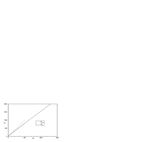
Figure 1: Energy-charge dependence for $Q$-balls. The upper and lower branches correspond to the thick-wall and thin-wall approximations, respectively.

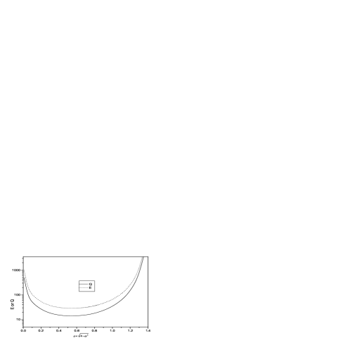
Figure 2: The energy and charge (obtained numerically) as functions of the parameter $\alpha=\sqrt{4-\omega^{2}}$.

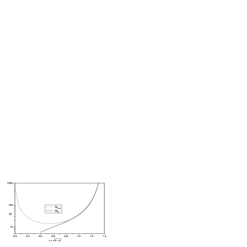
Figure 3: The charge $Q$ obtained numerically and semi-analytically (20) as a function of the parameter $\alpha=\sqrt{4-\omega^{2}}$.

Remark: The semi-Bogomolny method can be applied for other potentials of polynomial type. For example, in [12] the potential is of the form

$$U(f)=f^{2}\left[1+(1-f)^{2}\right]$$ (23)

and the corresponding semi-Bogomolny equation (analogous to (11)) is $f^{\prime}=-f(1-f)$ while its solution

$$f(r)=\frac{1}{1+\widetilde{C}_{{}_{B}}\,\exp(\sqrt{2}r)}.$$ (24)

has the same asymptotic behavior for large $r$ as in (12).

4 Woods-Saxon Ansatz

A more general form of the ansatz (12) is widely used in nuclear physics describing nuclear matter distribution inside heavy nuclei, or potential of nucleon-nucleus interaction. This is the so-called Woods-Saxon distribution and the corresponding profile function is given by

$$f(r)=\frac{C_{{}_{WS}}}{\sqrt{1+\exp\left[a\left(r-r_{{}_{{\tiny Q}}}\right)\right]}}.$$ (25)

In this case, three arbitrary parameters (instead of one) appear in the parametrization, and thus, more degrees of freedom exist. Here, $r_{{}_{Q}}$ corresponds to the radius of the Q-ball and $1/a$ defines the thickness of the shell of the Q-ball. At the origin, the values of the profile function and its derivative are: $f(0)=C_{{}_{WS}}\left(1+e^{-ar_{{}_{Q}}}\right)^{-1/2}$ and $f^{\prime}(0)=-a\,C_{{}_{WS}}e^{-ar_{{}_{Q}}}\left(2+2e^{-ar_{{}_{Q}}}\right)^{-3/2}$. Recall that, due to boundary conditions, $f^{\prime}(0)$ needs to be very small (in fact, zero). This limit can be obtained when the product $ar_{{}_{Q}}$ is large that is in the thin-wall approximation where $\omega\rightarrow\sqrt{2}$ (see below). The field-theoretical motivation for the Woods-Saxon ansatz was presented in the previous section since for $C_{{}_{WS}}=1$ and $C_{{}_{B}}=\exp(-ar_{{}_{Q}})$ the two profile functions given by (25) and (12) coincide.

For $Q$ large, the energy of the Q-balls given by (8-9) can be approximately evaluated using the Woods-Saxon ansatz (25). To do so, integrals of the following type are used:

$$I_{n} = \int\frac{\left(C_{{}_{WS}}\right)^{2n}}{\left(1+\exp\left[a(r-r_{{}_{{\tiny Q}}})\right]\right)^{n}}\,r^{2}\,dr$$ (26)

$$= \frac{1}{a^{3}}\,\left(C_{{}_{WS}}\right)^{2n}\left(b^{2}I_{n}^{0}+2b\,I_{n}^{1}+I_{n}^{2}\right)$$

where $n=1,2,3$ and $b=ar_{{}_{Q}}$ while the moment of inertia becomes: $I[f]=4\pi I_{1}$. In general, by letting $w=\exp[a(r-r_{{}_{Q}})]$ while $dr=dw/aw$, the $m$-power of the integral $I_{n}$ is defined as:

$$I_{n}^{m}=\int_{w_{0}}^{\infty}\frac{1}{z}\frac{(\ln\,w)^{m}}{(1+w)^{n}}\,dw$$ (27)

where $w_{0}=\exp(-b)$. After some algebra it can be easily shown that the integrals $I_{n}^{m}$ are related via the following recursive relation

$$I_{n+1}^{m}=I_{n}^{m}-{\frac{m}{n}}I_{n}^{m-1}-\frac{(\ln\,w_{0})^{m}}{n(1+w_{0})^{n}}.$$ (28)

For $w_{0}\ll 1$ one gets:

$$I_{1}^{0}\simeq b,\hskip 14.22636pt\hskip 14.22636pt\hskip 14.22636pt\hskip 14.22636pt\hskip 14.22636pt\!\!I_{2}^{0}\simeq b-1,\hskip 14.22636pt\hskip 14.22636pt\hskip 14.22636pt\hskip 14.22636pt\!\!I_{3}^{0}\simeq b-{\frac{3}{2}},$$

$$I_{1}^{1}\simeq-{\frac{b^{2}}{2}}+L,\hskip 14.22636pt\,\,\,\,\,\,I_{2}^{1}\simeq-{\frac{b^{2}}{2}}+L,\hskip 14.22636pt\hskip 14.22636pt\,\,\,\,\,I_{3}^{1}\simeq-{\frac{b^{2}}{2}}+L+{\frac{1}{2}},$$

$$I_{1}^{2}\simeq{\frac{b^{3}}{3}},\hskip 14.22636pt\hskip 14.22636pt\hskip 14.22636pt\hskip 14.22636pt\,\,I_{2}^{2}\simeq{\frac{b^{3}}{3}}-2L,\hskip 14.22636pt\hskip 14.22636pt\,\,\,\,\,I_{3}^{2}\simeq{\frac{b^{3}}{3}}-3L$$ (29)

where the parameter $L=2(1-1/4+1/9-1/16+...)\simeq 1.644$ does not contribute in the leading order expansion of the parameter $Q^{-1/3}$ (which we assume to be small – see below). Then the energy of the Q-ball (8 -9) can be approximated as

$$E_{{}_{Q}}\simeq\frac{Q^{2}}{\gamma 2VC_{{}_{WS}}^{2}}+\gamma VC_{{}_{WS}}^{2}\bigl{(}2-\alpha 2C_{{}_{WS}}^{2}+\beta C_{{}_{WS}}^{4}\bigr{)}+E_{deriv}$$ (30)

where $\alpha=1-3b^{-1}$, $\beta=1-\frac{9}{2}b^{-1}$, $\gamma=1+6Lb^{-2}$ and $V=\frac{4}{3}\pi r_{{}_{Q}}^{3}$. The derivative term of the energy: $E_{deriv}=\frac{1}{2}\int f^{\prime}{}^{2}\,r^{2}\,dr$ is going to be neglected (initially).

The minimization of $E_{{}_{Q}}$ with respect to $\gamma VC_{{}_{WS}}^{2}$ occurs at

$$(\gamma VC_{{}_{WS}}^{2})_{{}_{min}}=\frac{Q}{\sqrt{2(2-2C_{{}_{WS}}^{2}\alpha+C_{{}_{WS}}^{4}\beta)}}$$ (31)

which determines $r_{{}_{Q}}$. The corresponding minimum of the energy is

$$E_{{}_{Q}}\simeq\sqrt{2}Q\left(2-2\alpha C_{{}_{WS}}^{2}+\beta C_{{}_{WS}}^{4}\right).$$ (32)

Further minimization with respect to $C_{{}_{WS}}$ gives the following value for the energy

$$E_{{}_{Q}}\simeq\sqrt{2}Q\biggl{(}2-{\frac{\alpha^{2}}{\beta}}\biggr{)}$$ (33)

at $(C_{{}_{WS}})_{{}_{min}}^{2}=\alpha/\beta$. For large $b$ (of order $Q^{1/3}$), the parameter $(C_{{}_{WS}})_{{}_{min}}$ can be approximated by $(C_{{}_{WS}})_{{}_{min}}\simeq\sqrt{1+3/(2b)}=1+3/(4b)$ and in this limit the energy becomes:

$$E_{{}_{Q}}\simeq\sqrt{2}Q\left(1+{\frac{3}{4b}}\right)$$ (34)

where

$$(r_{{}_{Q}})_{{}_{min}}\simeq\biggl{(}{\frac{3}{4\sqrt{2}\pi}}\biggr{)}^{1/3}Q^{1/3}=0.55\,Q^{1/3}.$$ (35)

Note that equation (34) implies that $E_{{}_{Q}}\rightarrow\sqrt{2}Q$ as $b\to\infty$.

Next the derivative energy contribution is considered:

$$E_{deriv}\simeq\frac{a\pi C_{{}_{WS}}}{4}\left(r_{{}_{Q}}^{2}+\frac{2r_{{}_{Q}}}{a}+\frac{2L}{a^{2}}\right).$$ (36)

Taking into account the highest order terms in $r_{{}_{Q}}$ one obtains

$$E_{{}_{Q}}\simeq\sqrt{2}Q+{\frac{3Q}{2\sqrt{2}b}}+\frac{\pi b(r_{{}_{Q}})_{{}_{min}}}{4}.$$ (37)

Further minimization with respect to $b$ gives the energy-charge dependence of the Q-balls up to order $O(Q^{2/3})$:

$$E_{{}_{Q}} \simeq \sqrt{2}Q+\left(\frac{9\pi}{8\sqrt{2}}\right)^{1/3}Q^{2/3}$$ (38)

$$= \sqrt{2}\,Q+1.35702\,Q^{2/3}$$

which occurs when

$$b_{{}_{min}} = \biggl{(}{\frac{3\sqrt{2}Q}{\pi r_{{}_{{\tiny Q}}}}}\biggr{)}^{1/2}$$ (39)

$$= \left(\frac{12}{\pi}\,Q\right)^{1/3}\simeq 1.563\,Q^{1/3}.$$

Note that the $O(Q^{2/3})$ terms of (38) and (22) coincide, and therefore the two analytic methods are in good agreement. In addition, from (35) and since $b=ar_{{}_{Q}}$ one gets that $a_{{}_{min}}=2\sqrt{2}$ which is the value obtained from the semi-Bogomolny argument (12).

To conclude, let us state that in the thin-wall limit the profile function (25) is given by $f(0)\sim 1+3/(4b)$ (or by $f(0)\sim 1+1/(2b)$ including higher order corrections). Moreover, in this limit the Woods-Saxon distribution (25) is close to the exact values of the Q-ball profile function (obtained numerically) presented in Table 1. In fact, for $Q=149.26$: $f(0)=1.06$ and $f(0)_{{}_{num}}=1.0564$ while for $Q=722.66$: $f(0)=1.0356$ and $f(0)_{{}_{num}}=1.0345$.

Remark: For the alternative potential given by (23) the semi-Bogomolny function (24) can be generalized in a similar way as (25) and the corresponding energy is similar to (38) since

$$E_{{}_{Q}}\simeq\sqrt{2}Q+\left(\frac{\pi}{3\sqrt{2}}\right)^{1/3}Q^{2/3}.$$ (40)

Note that the two expressions differ only by a $2/3$ factor before the term $O(Q^{2/3})$.

5 Discussion and Conclusions

It has been shown that for specific parametrizations of the scalar field a semi-analytic treatment for Q-balls exists leading to transparent and simple results. Two kinds of approximations have been considered: one based on a semi-Bogomolny argument which gives an exponential-step parametrization for the profile function and the Woods-Saxon parametrization (the semi-Bogomolny generalization) motivated also by nuclear physics experience.

The agreement of the results obtained using both approximations with the numerical ones follows from the fact that the ansatz for the profile function obtained from semi-analytic approaches have the correct asymptotic behaviour as $Q$ and $r$ are large. This was not the case in the semi-analytic treatment of the Skyrme model in three or two spatial dimensions [14, 15]. Although the energies obtained were accurate within $0.5\%$ compared to the exact ones for large values of baryon number, the asymptotic behaviour of the profile function was incorrect [14].

The thickness of the Q-ball surface (ie transition region) where the profile $f$ decreases from $f\simeq 1$ to $f=0$ can be estimated by

$$t\simeq{\frac{2}{b}}\,r_{{}_{Q}}.$$ (41)

For $Q$ large (and using the results of section 4), the thickness is independent of the charge since $t\simeq\sqrt{2}$. Thus, the large Q-balls can be visualized as spherically symmetric balls with constant internal energy density

$$\rho_{{}_{E,V}}\simeq 2.$$ (42)

These balls are surrounded by a surface of constant thickness and constant average energy density per unit volume since

$$\rho_{{}_{E,S}} \simeq \frac{E_{deriv}}{4\pi t\,r_{{}_{Q}}^{2}}$$ (43)

$$= \frac{1}{4}$$

in natural units of the model. Therefore it is energetically favorable for small Q-balls to fuse into a bigger one since the surface of a single big Q-ball is smaller than the sum of surfaces of several smaller Q-balls, for the same value of $Q$ (or with the same total volume).

Our approach can be extended in lower (and also higher) spatial dimensions in a natural way. In particular, in the one-dimensional case the energy-charge dependence is

$$E(Q)_{{}_{1D}}\simeq\sqrt{2}Q+{\frac{1}{\sqrt{2}}}$$ (44)

which is in a close agreement (within $1\%$) with the numerical results obtained in [19]. In addition, the value of the profile function at the origin is (approximately) given by

$$f(0)_{{}_{1D}}\simeq 1+{\frac{1}{4Q}}$$ (45)

where terms of the form $\exp(-ar_{{}_{Q}})$ have been neglected since $Q$ is large (ie $r_{{}_{Q}}>>$).

In the two-dimensional case the corresponding results are

$$E(Q)_{{}_{2D}}\simeq\sqrt{2}Q+\biggl{(}{\frac{\pi}{2\sqrt{2}}}\biggr{)}^{1/2}\sqrt{Q}$$ (46)

while

$$f(0)_{{}_{2D}}\simeq 1+\left(\frac{\pi}{\sqrt{2}}\right)^{1/2}\frac{1}{4\sqrt{Q}}\,\cdot$$ (47)

The formulas (44), (46) and (38) indicate that the relative contribution of the surface energy ($E_{deriv}$) increases as the dimensionality of space increases. This property of Q-balls can be useful in cosmological applications. In some respect Q-balls are similar to the multiskyrmions which correspond to bubbles of matter with universal properties of the shell, where the mass and baryon number density is concentrated [14, 15].

We conclude by saying that our arguments can be extended to other types of potentials. Another important issue concerns the semi-analytic identification of the profile function satisfying equation (6) for (9). We expect to report on this problem soon.

References

• [1] S. Coleman, Nucl. Phys. B 262, 263 (1985)
• [2] T.D. Lee, Particle Physics and Introduction to Field Theory, Harwood, London (1981)
• [3] J.K. Drohm, L.P. Yok, Y.A. Simonov, J.A. Tyon and V.I. Veselov, Phys. Lett. B 101, 204 (1981)
• [4] T.I. Belova, A.E. Kudryavtsev, JETP 68, 7 (1989)
• [5] D.K. Hong, J. Low Temp. Phys. B 71, 483 (1998)
• [6] A. Kusenko, Phys. Lett. B 405, 108 (1997)
• [7] I. Affleck, M. Dine, Phys. Lett. B 249, 361 (1985)
• [8] A. Kusenko, M. Shaposhnikov, Phys. Lett. B 418, 46 (1998)
• [9] K. Enqvist, J. McDonald, Nucl. Phys. B 538, 321 (1999)
• [10] G. Rosen, J. Math. Phys. 9, 996 (1968)
• [11] M. Axenides, S. Komineas, L. Perivolaropoulos, M. Floratos, Phys. Rev. D 61, 085006 (2000)
• [12] T. Multamaki, I. Vilja, Nucl. Phys. B 574, 139 (2002); hep-ph/9908446
• [13] F. Paccetti Correia, M.G. Schmidt, Eur. Phys. J. C 21, 181 (2001); hep-th/0103189
• [14] V.B. Kopeliovich, JETP Lett. 73, 587 (2001); J. Phys. G 28, 103 (2002)
• [15] T.A. Ioannidou, V.B. Kopeliovich, W.J. Zakrzewski, JETP 95, 572 (2002); hep-th/0203253
• [16] A. Kusenko, Phys. Lett. B 404, 285 (1997)
• [17] E.B. Bogomolny, Sov. J. Nucl. Phys. 24, 449 (1976)
• [18] T.H.R. Skyrme, Nucl. Phys. 31, 556 (1962)
• [19] R.A. Battye, P.M. Sutcliffe, Nucl. Phys. B 590, 329 (2000)