OUTP–03–04P

hep-th/0302006

May 2002

Open Descendants of
NAHE–based free fermionic and Type I $\hbox{\mbmb Z}_{2}^{n}$ models
David J. Clements and Alon E. Faraggi
Theoretical Physics Department, University of Oxford, Oxford OX1 3NP

The NAHE–set, that underlies the realistic free fermionic models, corresponds to $\hbox{\mbm Z}_{2}\times\hbox{\mbm Z}_{2}$ orbifold at an enhanced symmetry point, with $(h_{11},h_{21})=(27,3)$. Alternatively, a manifold with the same data is obtained by starting with a $\hbox{\mbm Z}_{2}\times\hbox{\mbm Z}_{2}$ orbifold at a generic point on the lattice and adding a freely acting $\hbox{\mbm Z}_{2}$ involution. In this paper we study type I orientifolds on the manifolds that underly the NAHE–based models by incorporating such freely acting shifts. We present new models in the Type I vacuum which are modulated by $\hbox{\mbm Z}_{2}^{n}$ for $n=2,3$. In the case of $n=2$, the $\hbox{\mbm Z}_{2}\times\hbox{\mbm Z}_{2}$ structure is a composite orbifold Kaluza Klein shift arrangement. The partition function provides a simpler spectrum with chiral matter. For $n=3$, the case discussed is a $\hbox{\mbm Z}_{2}$ modulation of the $T^{6}/\hbox{\mbm Z}_{2}\times\hbox{\mbm Z}_{2}$ spectrum. The additional projection shows an enhanced closed and open sector with chiral matter. The brane stacks are correspondingly altered from those which are present in the $\hbox{\mbm Z}_{2}\times\hbox{\mbm Z}_{2}$ orbifold. In addition, we discuss the models arising from the open sector with and without discrete torsion.

1 Introduction

Important progress has been achieved in recent years in the basic understanding of string theory. It is now believed that the different string theories in ten dimensions, together with eleven dimensional supergravity, are limits of a single more fundamental theory, traditionally called M–theory. The question remains, however, how to relate these advances to experimental data. In this context some efforts have been directed at the construction of phenomenologically viable type I string vacua [1], and nonperturbative M–theory vacua based on compactifications of 11 dimensional supergravity on CY$\times S_{1}/\hbox{\mbm Z}_{2}$ [2, 3, 5] or on manifolds with $G_{2}$ holonomy [6].

These perturbative string constructions, however, do not yet utilize the new M–theory picture of string theories. The question remains how to employ this new understanding for phenomenological studies. In the context of M–theory the true fundamental theory of nature should have some nonperturbative realization. However, at present all we know about this more basic theory are its perturbative string limits. Therefore, we should regard these theories as providing tools to probe the properties of the fundamental nonperturbative vacuum in the different limits. Each of the perturbative string limits may therefore exhibit some properties of the true vacuum, but it may well be that none can characterize the vacuum completely. In this view it is likely that all limits will need to be used to isolate the true M–theory vacuum. In this respect it may well be that different perturbative string limits may provide more useful means to study different properties of the true nonperturbative vacuum. This suggests the following approach to exploration of M–theory phenomenology. Namely, the true M–theory vacuum has some nonperturbative realization that at present we do not know how to formulate. This vacuum is at finite coupling and is located somewhere in the space of M–theory vacua. The properties of the true vacuum can however be probed in the perturbative string limits. We may hypothesize that in any of these limits one still needs to compactify to four dimensions. Namely, that the true M–theory vacuum can still be formulated with four non–compact and all the other dimensions are compact. Suppose then that in some of the limits we are able to identify a specific class of compactifications that possess appealing phenomenological properties. The new M–theory picture suggests that we can then explore the possible properties of the M–theory vacuum by studying compactifications of the other perturbative string limits on the same class of compactifications.

In particular, we can probe those properties that pertain to the observed experimental and cosmological data, and by using the low energy effective field theory parameterization. One of these properties, indicated by the observed data, is the embedding of the Standard Model matter states in the chiral ${\bf 16}$ representation of $SO(10)$. Thus, we may demand the existence of a viable perturbative string limit which preserve this embedding. The only perturbative string limit which enables the $SO(10)$ embedding of the Standard Model spectrum is the heterotic $E_{8}\times E_{8}$ string. The reason being that only this limit produces the spinorial 16 representation in the perturbative massless spectrum. Therefore, if we would like to preserve the $SO(10)$ embedding of the Standard Model spectrum, the M–theory limit which we should use is the perturbative heterotic string [7]. In this respect it may well be that other perturbative string limits may provide more useful means to study different properties of the true nonperturbative vacuum, such as dilaton and moduli stabilization [8].

Pursuing this point of view, a class of realistic string models that preserve the $SO(10)$ embedding of the Standard Model spectrum are the NAHE–based free fermionic models. This formulation enables detailed studies at fixed points in the moduli space, and the models under consideration correspond to $\hbox{\mbm Z}_{2}\times\hbox{\mbm Z}_{2}$ orbifold compactifications with additional Wilson lines. Many of the encouraging phenomenological characteristics of the realistic free fermionic models are rooted in the underlying $\hbox{\mbm Z}_{2}\times\hbox{\mbm Z}_{2}$ orbifold structure, including the three generations arising from the three twisted sectors, and the canonical SO(10) embedding for the weak hyper-charge. We may therefore regard the phenomenological success of the free fermionic models as highlighting a specific class of compactified manifolds.

Given the specific class of compactified manifolds highlighted by NAHE–based free fermionic models, the line of approach to phenomenological studies of M–theory that we pursue here is to compactify other perturbative string limits on the same manifolds. It is then hoped that these studies will elucidate other properties of these realistic models. This is the line of thought that was pursued in ref. [5] where compactification of Horava–Witten theory to four dimensions on manifolds that are related to the free fermionic models were studied.

Pursuing this approach we study in this paper orientifolds of type IIB string theory on the manifolds that are related to the free fermionic models. The geometric manifold that underlies the free fermionic models is a $\hbox{\mbm Z}_{2}\times\hbox{\mbm Z}_{2}$ orbifold at an enhanced symmetry point in the Narain moduli space. At the free fermionic point the Narain lattice arising from the six compactified dimensions is enhanced from $U(1)^{6}$ to $SO(12)$. The $\hbox{\mbm Z}_{2}\times\hbox{\mbm Z}_{2}$ orbifold projection of this lattice then yields a manifold with $(h_{11},h_{21})=(27,3)$. On the other hand a $\hbox{\mbm Z}_{2}\times\hbox{\mbm Z}_{2}$ orbifold projection at a generic point in the moduli space yields a manifold with $(h_{21},h_{11})=(51,3)$. We refer to the later as $X_{1}$ and to the former as $X_{2}$. These two manifolds can alternatively be connected by adding a freely acting shift to $X_{1}$, which reduces the number of twisted fixed points by 1/2. Orientifolds of $\hbox{\mbm Z}_{2}\times\hbox{\mbm Z}_{2}$ orbifolds were studied in ref. [9]. To advance these studies toward nonperturbative studies of the free fermionic models we therefore extend this analysis by including the freely acting shift that connects the $X_{1}$ and $X_{2}$ manifolds.

2 Realistic free fermionic models - general structure

In this section we recapitulate the main structure of the realistic free fermionic models. The notation and details of the construction of these models are given elsewhere [10]. In the free fermionic formulation [11] of the heterotic string in four dimensions a model is specified in terms of boundary condition basis vectors and one–loop GSO phases. The physical spectrum is obtained by applying the generalized GSO projections. The boundary condition basis defining a typical realistic free fermionic heterotic string models is constructed in two stages. The first stage consists of the NAHE set, which is a set of five boundary condition basis vectors, $\{{\bf 1},S,b_{1},b_{2},b_{3}\}$ [12]. The gauge group after imposing the GSO projections induced by the NAHE set is $SO(10)\times SO(6)^{3}\times E_{8}$ with $N=1$ supersymmetry. At the level of the NAHE set the sectors $b_{1}$, $b_{2}$ and $b_{3}$ produce 48 multiplets, 16 from each, in the $16$ representation of $SO(10)$. The states from the sectors $b_{j}$ are singlets of the hidden $E_{8}$ gauge group and transform under the horizontal $SO(6)_{j}$ $(j=1,2,3)$ symmetries. This structure is common to all the realistic free fermionic models.

The second stage of the basis construction consists of adding to the NAHE set three (or four) additional boundary condition basis vectors, typically denoted by $\{\alpha,\beta,\gamma\}$. These additional basis vectors reduce the number of generations to three chiral generations, one from each of the sectors $b_{1}$, $b_{2}$ and $b_{3}$, and simultaneously break the four dimensional gauge group. The assignment of boundary conditions breaks $SO(10)$ to one of its subgroups [10]. Similarly, the hidden $E_{8}$ symmetry is broken to one of its subgroups by the basis vectors which extend the NAHE set. The flavor $SO(6)^{3}$ symmetries in the NAHE–based models are broken to flavor $U(1)$ symmetries. The three additional basis vectors $\{\alpha,\beta,\gamma\}$ differ between the models and there exists a large number of viable three generation models in this class.

From the preceding discussion it follows that the underlying $\hbox{\mbm Z}_{2}\times\hbox{\mbm Z}_{2}$ orbifold structure is common to all the three generation free fermionic models. This is the structure that we will exploit in trying to elevate the study of these models across the strong–weak duality barrier. In this respect our aim is to explore which of the structures of these models is preserved in the nonperturbative domain. We should note that a priori – we have no clue – and therefore the analysis is purely exploratory.

The correspondence of the NAHE–based free fermionic models with the orbifold construction is illustrated by extending the NAHE set, $\{{\bf 1},S,b_{1},b_{2},b_{3}\}$, by one additional boundary condition basis vector [13], $\xi_{1}$. With a suitable choice of the GSO projection coefficients the model possess an $SO(4)^{3}\times E_{6}\times U(1)^{2}\times E_{8}$ gauge group and $N=1$ space–time supersymmetry. The matter fields include 24 generations in the 27 representations of $E_{6}$, eight from each of the sectors $b_{1}\oplus b_{1}+\xi_{1}$, $b_{2}\oplus b_{2}+\xi_{1}$ and $b_{3}\oplus b_{3}+\xi_{1}$. Three additional 27 and $\overline{27}$ pairs are obtained from the Neveu–Schwarz $\oplus~{}\xi_{1}$ sector.

To construct the model in the orbifold formulation one starts with a model compactified on a flat torus with nontrivial background fields [14]. The subset of basis vectors

$$\{{\bf 1},S,\xi_{1},\xi_{2}\},$$ (2.1)

with $\xi_{2}={\bf 1}+b_{1}+b_{2}+b_{3}$, generates a toroidally-compactified model with $N=4$ space–time supersymmetry and $SO(12)\times E_{8}\times E_{8}$ gauge group. The same model is obtained in the geometric (bosonic) language by constructing the background fields which produce the $SO(12)$ lattice. The metric of the six-dimensional compactified manifold is taken as the Cartan matrix of $SO(12)$, and the antisymmetric tensor is given by

$$B_{ij}=\cases{G_{ij}&;\ $i>j$,\cr 0&;\ $i=j$,\cr-G_{ij}&;\ $i<j$.\cr}$$ (2.2)

When all the radii of the six-dimensional compactified manifold are fixed at $R_{I}=\sqrt{2}$, it is seen that the left– and right–moving momenta $P^{I}_{R,L}=[m_{i}-{1\over 2}(B_{ij}{\pm}G_{ij})n_{j}]{e_{i}^{I}}^{*}$reproduce all the massless root vectors in the lattice of $SO(12)$. Here $e^{i}=\{e_{i}^{I}\}$ are six linearly-independent vectors normalized: $(e_{i})^{2}=2$. The ${e_{i}^{I}}^{*}$ are dual to the $e_{i}$, with $e_{i}^{*}\cdot e_{j}=\delta_{ij}$.

Adding the two basis vectors $b_{1}$ and $b_{2}$ to the set (2.1) corresponds to the $\hbox{\mbm Z}_{2}\times\hbox{\mbm Z}_{2}$ orbifold model with standard embedding. Starting from the Narain model with $SO(12)\times E_{8}\times E_{8}$ symmetry [14], and applying the $\hbox{\mbm Z}_{2}\times\hbox{\mbm Z}_{2}$ twisting on the internal coordinates, reproduces the spectrum of the free-fermion model with the six-dimensional basis set $\{{\bf 1},S,\xi_{1},\xi_{2},b_{1},b_{2}\}$. The Euler characteristic of this model is 48 with $h_{11}=27$ and $h_{21}=3$.

It is noted that the effect of the additional basis vector $\xi_{1}$ is to separate the gauge degrees of freedom from the internal compactified degrees of freedom. In the realistic free fermionic models this is achieved by the vector $2\gamma$ [13], which breaks the $E_{8}\times E_{8}$ symmetry to $SO(16)\times SO(16)$. The $\hbox{\mbm Z}_{2}\times\hbox{\mbm Z}_{2}$ twisting breaks the gauge symmetry to $SO(4)^{3}\times SO(10)\times U(1)^{3}\times SO(16)$. The orbifold twisting still yields a model with 24 generations, eight from each twisted sector, but now the generations are in the chiral 16 representation of $SO(10)$, rather than in the 27 of $E_{6}$. The same model can be realized with the set $\{{\bf 1},S,\xi_{1},\xi_{2},b_{1},b_{2}\}$, by projecting out the $16\oplus{\overline{16}}$ from the sector $\xi_{1}$ by taking

$$c{\xi_{1}\choose\xi_{2}}\rightarrow-c{\xi_{1}\choose\xi_{2}}.$$ (2.3)

This choice also projects out the massless vector bosons in the 128 of $SO(16)$ in the hidden-sector $E_{8}$ gauge group, thereby breaking the $E_{6}\times E_{8}$ symmetry to $SO(10)\times U(1)\times SO(16)$. The freedom in eq. (2.3) correspond to a discrete torsion in the toroidal orbifold model. At the level of the $N=4$ Narain model generated by the set (2.1), we can define two models, $Z_{+}$ and $Z_{-}$, depending on the sign of the discrete torsion in eq. (2.3). One model, say $Z_{+}$, produces the $E_{8}\times E_{8}$ model, whereas the second, say $Z_{-}$, produces the $SO(16)\times SO(16)$ model. However, the $\hbox{\mbm Z}_{2}\times\hbox{\mbm Z}_{2}$ twists act identically in the two models, and their physical characteristics differ only due to the discrete torsion eq. (2.3).

This analysis confirms that the $\hbox{\mbm Z}_{2}\times\hbox{\mbm Z}_{2}$ orbifold on the $SO(12)$ Narain lattice is indeed at the core of the realistic free fermionic models. However, this orbifold model differs from the $\hbox{\mbm Z}_{2}\times\hbox{\mbm Z}_{2}$ orbifold on $T_{2}^{1}\times T_{2}^{2}\times T_{2}^{3}$ with $(h_{11},h_{21})=(51,3)$. In ref. [15] it was shown that the two models are connected by adding a freely acting twist or shift to the $X_{1}$ model. Let us first start with the compactified $T^{1}_{2}\times T^{2}_{2}\times T^{3}_{2}$ torus parameterized by three complex coordinates $z_{1}$, $z_{2}$ and $z_{3}$, with the identification

$$z_{i}=z_{i}+1~{}~{}~{}~{}~{}~{}~{}~{}~{}~{};~{}~{}~{}~{}~{}~{}~{}~{}~{}~{}z_{i}=z_{i}+\tau_{i}$$ (2.4)

where $\tau$ is the complex parameter of each $T_{2}$ torus. With the identification $z_{i}\rightarrow-z_{i}$, a single torus has four fixed points at

$$z_{i}=\{0,1/2,\tau/2,(1+\tau)/2\}.$$ (2.5)

With the two $\hbox{\mbm Z}_{2}$ twists

$$\alpha:(z_{1},z_{2},z_{3})\rightarrow(-z_{1},-z_{2},~{}~{}z_{3})$$ (2.6)

$$\beta:(z_{1},z_{2},z_{3})\rightarrow(~{}~{}z_{1},-z_{2},-z_{3}),$$ (2.7)

there are three twisted sectors in this model, $\alpha$, $\beta$ and $\alpha\beta=\alpha\cdot\beta$, each producing 16 fixed tori, for a total of 48. Adding to the model generated by the $\hbox{\mbm Z}_{2}\times\hbox{\mbm Z}_{2}$ twists in (2.7), the additional shift

$$\gamma:(z_{1},z_{2},z_{3})\rightarrow(z_{1}+{1\over 2},z_{2}+{1\over 2},z_{3}+{1\over 2})$$ (2.8)

produces again a fixed tori from the three twisted sectors $\alpha$, $\beta$ and $\alpha\beta$. The product of the $\gamma$ shift in (2.8) with any of the twisted sectors does not produce any additional fixed tori. Therefore, this shift acts freely. Under the action of the $\gamma$ shift, half the fixed tori from each twisted sector are paired. Therefore, the action of this shift is to reduce the total number of fixed tori from the twisted sectors by a factor of $1/2$, with $(h_{11},h_{21})=(27,3)$. This model therefore reproduces the data of the $\hbox{\mbm Z}_{2}\times\hbox{\mbm Z}_{2}$ orbifold at the free-fermion point in the Narain moduli space.

We noted above that the freely acting shift (2.8), added to the ${\hbox{\mbm Z}}_{2}\times{\hbox{\mbm Z}}_{2}$ orbifold at a generic point of $T_{2}^{1}\times T_{2}^{2}\times T_{2}^{3}$, reproduces the data of the ${\hbox{\mbm Z}}_{2}\times{\hbox{\mbm Z}}_{2}$ orbifold acting on the SO(12) lattice. This observation does not prove, however, that the vacuum which includes the shift is identical to the free fermionic model. While the massless spectrum of the two models may coincide their massive excitations, in general, may differ. The matching of the massive spectra is examined by constructing the partition function of the ${\hbox{\mbm Z}}_{2}\times{\hbox{\mbm Z}}_{2}$ orbifold of an SO(12) lattice, and subsequently that of the model at a generic point including the shift. In effect since the action of the ${\hbox{\mbm Z}}_{2}\times{\hbox{\mbm Z}}_{2}$ orbifold in the two cases is identical the problem reduces to proving the existence of a freely acting shift that reproduces the partition function of the SO(12) lattice at the free fermionic point. Then since the action of the shift and the orbifold projections are commuting it follows that the two ${\hbox{\mbm Z}}_{2}\times{\hbox{\mbm Z}}_{2}$ orbifolds are identical.

On the compact coordinates there are actually three inequivalent ways in which the shifts can act. In the more familiar case, they simply translate a generic point by half the length of the circle. As usual, the presence of windings in string theory allows shifts on the T-dual circle, or even asymmetric ones, that act both on the circle and on its dual. More concretely, for a circle of length $2\pi R$, one can have the following possibilities [16]:

$$A_{1}\;: X_{\rm L,R}\to X_{\rm L,R}+{\textstyle{1\over 2}}\pi R\,,$$

$$A_{2}\;: X_{\rm L,R}\to X_{\rm L,R}+{\textstyle{1\over 2}}\left(\pi R\pm{\pi\alpha^{\prime}\over R}\right)\,,$$

$$A_{3}\;: X_{\rm L,R}\to X_{\rm L,R}\pm{\textstyle{1\over 2}}{\pi\alpha^{\prime}\over R}\,.$$ (2.9)

There is an important difference between these choices: while $A_{1}$ and $A_{3}$ can act consistently on any number of coordinates, level-matching requires instead that $A_{2}$ acts on (mod) four real coordinates. By studying the respective partition function one finds [17] that the shift that reproduces the $SO(12)$ lattice at the free fermionic point in the moduli space is generated by the ${\hbox{\mbm Z}}_{2}\times{\hbox{\mbm Z}}_{2}$ shifts

$$g\;: (A_{2},A_{2},0)\,,$$

$$h\;: (0,A_{2},A_{2})\,,$$ (2.10)

where each $A_{2}$ acts on a complex coordinate. It is then shown that the partition function of the SO(12) lattice is reproduced. at the self-dual radius, $R_{i}=\sqrt{\alpha^{\prime}}$. On the other hand, the shifts given in Eq. (2.8), and similarly the analogous freely acting shift given by $(A_{3},A_{3},A_{3})$, do not reproduce the partition function of the $SO(12)$ lattice. Therefore, the shift in eq. (2.8) does reproduce the same massless spectrum and symmetries of the ${\hbox{\mbm Z}}_{2}\times{\hbox{\mbm Z}}_{2}$ at the free fermionic point, but the partition functions of the two models differ! Thus, the free fermionic ${\hbox{\mbm Z}}_{2}\times{\hbox{\mbm Z}}_{2}$ is realized for a specific form of the freely acting shift given in eq. (2.10). However, all the models that are obtained from $X_{1}$ by a freely acting ${\hbox{\mbm Z}}_{2}$-shift have $(h_{11},h_{21})=(27,3)$ and hence are connected by continuous extrapolations. The study of these shifts in themselves may therefore also yield additional information on the vacuum structure of these models and is worthy of exploration.

Despite its innocuous appearance the connection between $X_{1}$ and $X_{2}$ by a freely acting shift has the profound consequence of making the $X_{2}$ manifold non–simply connected, which allows the breaking of the SO(10) symmetry to one of its subgroups. Thus, we can regard the utility of the free fermionic machinery as singling out a specific class of $\hbox{\mbm Z}_{2}\times\hbox{\mbm Z}_{2}$ compactified manifolds. In this context the freely acting shift has the crucial function of connecting between the simply connected covering manifold to the non-simply connected manifold. Precisely such a construction has been utilized in [3, 5] to construct non-perturbative vacua of heterotic M-theory. In the next section we turn to study open descendants of $\hbox{\mbm Z}_{2}\times\hbox{\mbm Z}_{2}$ orbifolds that incorporate such freely acting shifts.

3 $\hbox{\mbmbb Z}_{2}\times\hbox{\mbmbb Z}_{2}$ Model With Composite Shift Orbifold Generators

To illustrate the effects of the freely acting shifts of the type in eq. (2.8) on the open descendants, we start with a simpler example of a $\hbox{\mbm Z}_{2}$ orbifold, $g$ and an additional freely acting shift $h$. The action of $g$ and $h$ and their products is given in eq. (3).

The $\hbox{\mbm Z}_{2}\times\hbox{\mbm Z}_{2}$ generators have both an action on the string coordinates (as a parity projection), and the topology of the internal directions, in that they break $T^{6}$ to $T^{2}_{45}\times T^{2}_{67}\times T^{2}_{89}$, with subscripts referring to the 2-tori directions. As such, the original type IIB theory is projected using

$$g = (1~{},~{}1;-1~{},-1;-1,-1~{}),$$

$$h = (A_{1},1;~{}A_{1}~{},~{}1~{};~{}~{}1~{},~{}1~{}),$$

$$f = (A_{1},1;-A_{1},-1;-1,-1),$$ (3.1)

for $A_{1}$ defined in (2.9). The generators, (3) illustrates the shift action on only one of the coordinates of the relevant torus. The orbifolds act on all coordinates within a given torus to provide four fixed points.

This is an interesting model that has a $\hbox{\mbm Z}_{2}\times\hbox{\mbm Z}_{2}$ structure while preserving ${\cal N}=2$ supersymmetry. The choice of generators that has at least two with shift operators, has the effect of shifting elements of a matrix $M$ (which encodes the positions of the fixed points)

$$TrhMq^{L_{0}}q^{\bar{L}_{0}}$$ (3.2)

to the off diagonal positions in the torus amplitude. This implies that the independent orbit diagrams (those not related by modular transformation) no longer contribute to the torus amplitude. This takes away the consideration of a sub class of models associated with a sign freedom. As will be shown, sign changes arising from the discrete torsion terms will necessarily change the charge of the brane that they couple to, in addition to fundamentally changing the partition function for the overall sign of the product of signs $\epsilon_{k}=\pm 1$.

The way the modulating group generators are written with composite shift operators, has a twofold effect, firstly it will necessarily force the number of distinct $D5$ embedding types to become only one (in this case, the first torus will provide the $D5$ physics). This happens because the lifting of lattice states for a given direction by the action of a shift operation forces the tadpole condition to eliminate the corresponding brane, as discussed also in [4]. Secondly, the particular arrangement of the shifted directions will allow for an interesting geometrical configuration of the $O$-planes in the Klein amplitude.

¿From (3), it is appreciated that the vacuum is left with 2 degrees of freedom in the $R$-$R$ sector. This is easily seen by appreciating that an orbifold projection acts as a $\pi$ rotation under $SU(2)$ generators on the moduli. Which in this case, the orbifold operation effects only two of the internal directions. The model thus has an ${\cal N}=2$ supersymmetry.

The ${\cal N}=2$ character set is derived from the breaking of the original SO(8) lightcone characters $O_{8}$, $V_{8}$, $C_{8}$ and $S_{8}$ to supersymmetric representations involving $O_{4}$, $V_{4}$, $C_{4}$ and $S_{4}$. The type I constructions are discussed in detail in [18]. In this case, the supersymmetric world sheet fermion contributions are written as

$Q_{o}=V_{4}O_{4}-C_{4}C_{4}$,	$Q_{v}=O_{4}V_{4}-S_{4}S_{4}$
$Q_{s}=O_{4}C_{4}-S_{4}O_{4}$,	$Q_{c}=V_{4}S_{4}-C_{4}V_{4}$.

The $SO(2n)$ characters are,

$O_{2n}=\frac{1}{2\eta^{n}}\big{(}\theta^{n}_{3}+\theta^{n}_{4}\big{)}$,	$V_{2n}=\frac{1}{2\eta^{n}}\big{(}\theta^{n}_{3}-\theta^{n}_{4}\big{)}$,
$S_{2n}=\frac{1}{2\eta^{n}}\big{(}\theta^{n}_{2}+i^{-n}\theta^{n}_{1}\big{)}$	$C_{2n}=\frac{1}{2\eta^{n}}\big{(}\theta^{n}_{2}-i^{-n}\theta^{n}_{1}\big{)}$.

with the Dedekind eta function

$$\eta=q^{\frac{1}{24}}\prod_{n=1}^{\infty}\big{(}1-q^{n}\big{)},$$

their respective conformal weights are $0$, $\frac{1}{2}$, $\frac{n}{8}$ and $\frac{n}{8}$. Here, these are representations of a scalar, a vector, and spinors of opposite chirality. The theta functions originate from the $NS$ and $R$ sectors and are defined by

$$\theta\left[\matrix{\chi\cr\phi\cr}\right]=\sum_{n}q^{\frac{1}{2}(n+\chi)^{2}}e^{2\pi i(n+\chi)\phi}$$ (3.3)

where $\chi$ and $\phi$ take the values $\frac{1}{2}$ $(NS)$ and $0$ $(R)$, the labelled theta functions are then defined as,

$$\theta_{1}=\left[\matrix{\frac{1}{2}\cr\frac{1}{2}\cr}\right],\quad\theta_{2}=\left[\matrix{\frac{1}{2}\cr 0\cr}\right],\quad\theta_{3}=\left[\matrix{0\cr 0\cr}\right]\quad{\rm and}\quad\theta_{4}=\left[\matrix{0\cr\frac{1}{2}\cr}\right].$$ (3.4)

We will use a compact notation for the lattice modes arising from the compactification on a torus. In a given direction of a torus, one has a lattice of the form

$$\Lambda_{m+a,n+b}=\frac{q^{\frac{\alpha\prime}{4}{\big{(}\frac{(m+a)}{R}+\frac{(n+b)R}{\alpha\prime}\big{)}}^{2}}\bar{q}^{\frac{\alpha\prime}{4}{\big{(}\frac{(m+a)}{R}-\frac{(n+b)R}{\alpha\prime}\big{)}}^{2}}}{\eta(q)\eta(\bar{q})}.$$

Where the values $a$ and $b$ are in anticipation of the effect of winding or momentum shifts under $S$ transformation.

To obtain modular invariance under $SL(2,\hbox{\mbm Z})$, as required by the topology of the one loop string amplitude, one must perform $S$ and $T$ transforms, the generators of this group, which act on the complex torus covering parameter $\tau$ as

$$S:\tau\rightarrow-\frac{1}{\tau} \Rightarrow(a,b)\rightarrow(b,a^{-1})$$

$$T:\tau\rightarrow\tau+1 \Rightarrow(a,b)\rightarrow(a,ab)$$

Here, $a$ and $b$ label the orbifold/twist operations that are placed on two sides of the torus sheet. The full orbit configuration of these operators is described for the $\hbox{\mbm Z}_{2}\times\hbox{\mbm Z}_{2}$ case in 4.

Lattice	${\cal A}$	${\cal K}~{}$and$~{}{\cal M}$
$P_{m}$	$W_{n}$	$W_{2n}$
$(-1)^{m}P_{m+\frac{1}{2}}$	$(-1)^{n}W_{n+\frac{1}{2}}$	$(-1)^{n}W_{2n+1}$
$P_{m+\frac{1}{2}}$	$(-1)^{n}W_{n}$	$(-1)^{n}W_{2n}$
$(-1)^{m}P_{m}$	$W_{n+\frac{1}{2}}$	$W_{2n+1}$

Table 1: Lattice $S$ transforms

Here, ${\cal A}$, ${\cal K}$ and ${\cal M}$ are the annulus Klein and Mobius contributions, and the relevant terms can be seen by using the appropriate form for the measure parameter in each case. $P$ and $W$ are the restriction of $\Lambda_{m,n}$ to pure Kaluza-Klein ($P$) or winding ($W$) modes. The further notation of $P_{o}$ and $P_{e}$ (and similarly for the winding sums) are the restriction of the counting to even or odd modes only. In the case of odd lattices, the convention should not be taken to be correlated with labels on the fermionic contributions. The action on these lattice modes for $S$ transformations are as in table 1. The action of $T$ on the lattices are

$$\begin{array}[]{lcl}\Lambda_{m,n}\rightarrow\Lambda_{m,n},&&\Lambda_{m,n+\frac{1}{2}}\rightarrow(-1)^{m}\Lambda_{m,n+\frac{1}{2}},\\ \Lambda_{m+\frac{1}{2},n}\rightarrow(-1)^{n}\Lambda_{m+\frac{1}{2},n},&{\rm and}&\Lambda_{m+\frac{1}{2},n+\frac{1}{2}}\rightarrow i(-1)^{m+n}\Lambda_{m+\frac{1}{2},n+\frac{1}{2}}.\end{array}$$

Thus the modular invariant torus amplitude is

$${\cal T}= \frac{1}{4} \bigg{\{}\big{[}1+(-1)^{m_{1}+m_{2}}\big{]}(\Lambda^{1}\Lambda^{2}+\Lambda^{1}_{m,n+\frac{1}{2}}\Lambda^{2}_{m,n+\frac{1}{2}})\Lambda^{3}|Q_{o}+Q_{v}|^{2}$$

$$+\big{[}1+(-1)^{m_{1}}\big{]}\Lambda^{1}|Q_{o}-Q_{v}|^{2}{\vline\frac{2\eta}{\theta_{2}}\vline}^{4}$$

$$+16(\Lambda^{1}+\Lambda^{1}_{m,n+\frac{1}{2}}){\vline\frac{\eta}{\theta_{4}}\vline}^{4}|Q_{s}+Q_{c}|^{2}$$

$$+16(\Lambda^{1}+(-1)^{m_{1}}\Lambda^{1}_{m,n+\frac{1}{2}}){\vline\frac{\eta}{\theta_{3}}\vline}^{4}|Q_{s}-Q_{c}|^{2}\bigg{\}}.$$

With the $A_{1}$ shift operator, the number of fixed points can be seen to be halved, it acts on the fixed point coordinates as

$$(0,0;0,0)\rightarrow(0+\frac{1}{2},0;0+\frac{1}{2},0).$$ (3.9)

Where the labelling $(x_{2},y_{2};x_{3},y_{3})$ defines the collective fixed point coordinate for the space $T^{2}_{67}\times T^{2}_{89}$, for the values $\{x_{i},y_{i}|x_{i}\in\{0,\frac{1}{2}\},y_{i}\in\{0,\frac{1}{2}\}\}$. The total number of fixed points without the shift operation is $16=4\times 4$, which are detailed in table (2).

${(0,0;0,0)}_{1}$	${(0,\frac{1}{2};0,0)}_{2}$	${(\frac{1}{2},0;0,0)}_{3}$	${(\frac{1}{2},\frac{1}{2};0,0)}_{4}$
${(0,0;0,\frac{1}{2})}_{5}$	${(0,0;\frac{1}{2},0)}_{6}$	${(0,0;\frac{1}{2},\frac{1}{2})}_{7}$	${(0,\frac{1}{2};0,\frac{1}{2})}_{8}$
${(0,\frac{1}{2};\frac{1}{2},0)}_{9}$	${(0,\frac{1}{2};\frac{1}{2},\frac{1}{2})}_{10}$	${(\frac{1}{2},0;0,\frac{1}{2})}_{11}$	${(\frac{1}{2},0;\frac{1}{2},0)}_{12}$
${(\frac{1}{2},0;\frac{1}{2},\frac{1}{2})}_{13}$	${(\frac{1}{2},\frac{1}{2};0,\frac{1}{2})}_{14}$	${(\frac{1}{2},\frac{1}{2};\frac{1}{2},0)}_{15}$	${(\frac{1}{2},\frac{1}{2};\frac{1}{2},\frac{1}{2})}_{16}$

Table 2: Unshifted fixed points

The origin of the lattice contributions of the torus amplitude

$${\cal T}_{0}=|Q_{o}|^{2}+|Q_{v}|^{2}+8|Q_{s}|^{2}+\ldots.$$ (3.10)

shows, as expected, 8 fixed points, reduced from 16 within a given orbifold projection, the independent coordinates of which are as in table 3.

${(0,0;0,0)}_{1}$	${(0,\frac{1}{2};0,0)}_{2}$	${(\frac{1}{2},0;0,0)}_{3}$	${(\frac{1}{2},\frac{1}{2};0,0)}_{4}$
${(0,0;0,\frac{1}{2})}_{5}$	${(0,0;\frac{1}{2},\frac{1}{2})}_{7}$	${(0,\frac{1}{2};0,\frac{1}{2})}_{8}$	${(0,\frac{1}{2};\frac{1}{2},\frac{1}{2})}_{10}$

Table 3: Remaining fixed points

Vertex operators of states flowing in $K$ and $\tilde{{\cal A}}$ will acquire from the torus, by virtue of the action of the shift in $T_{45}^{2}$ and $T_{67}^{2}$, a state projector

$$V=\big{[}1+(-1)^{m_{1}+m_{2}}\big{]}V_{(T^{4}/\hbox{\ssmbm Z}_{2})\times T_{2}}.$$ (3.11)

The torus amplitude in the type I setting is accompanied by the Klein bottle amplitude, which is realized from the type IIB projection

$$Tr_{IIB}\frac{(1+\Omega)}{2}q^{L_{0}}{\bar{q}}^{\tilde{L}_{0}}.$$ (3.12)

Where $\Omega$ has the usual definition of the world sheet parity operator. Terms contributing to the Klein correspond to those terms in the trace with the $\Omega$ insertion.

$\Omega$ makes an effective identification of the left and right modes. As such, orbifold elements acting on the world sheet bosonic or fermionic oscillators are made ineffective by $\Omega$. This is easily seen by series expansion of such terms, since the left and right modes contribute $(-1)^{k+\tilde{k}}$, $k,\tilde{k}\in\hbox{\mbm Z}$, the identification then neglects the orbifold presence.

In a similar fashion, this projection also reduces the lattice modes to become either pure momentum or pure winding, this situation is inverted with the assistance of an inserted orbifold action $\alpha$:

$$\Omega|p_{L},p_{R}> = |p_{R},p_{L}>\quad\Rightarrow\quad n=0,$$

$$\Omega\alpha|p_{L},p_{R}> = |-p_{R},-p_{L}>\quad\Rightarrow\quad m=0.$$ (3.13)

$\Omega$ has no effect on the twisting operations, since these are realized as a shift in the oscillator modes. Thus, the Klein amplitude takes the form,

$${\cal K}= \frac{1}{8} \bigg{\{}\bigg{[}\big{(}1+(-1)^{m_{1}+m_{2}}\big{)}P_{1}P_{2}P_{3}$$ (3.14)

$$+\big{(}1+(-1)^{m_{1}}\big{)}P_{1}W_{2}W_{3}\bigg{]}(Q_{o}+Q_{v})$$

$$+32(Q_{s}+Q_{c})P_{1}{\bigg{(}\frac{\eta}{\theta_{4}}\bigg{)}}^{2}\bigg{\}}$$

With corresponding transverse amplitude

$$\tilde{{\cal K}}= \frac{2^{5}}{8} \bigg{\{}\bigg{[}(W_{1}^{e}W_{2}^{e}+W_{1}^{o}W_{2}^{o})W_{3}^{e}v_{1}v_{2}v_{3}+W_{1}P_{2}^{e}P_{3}^{e}\frac{v_{1}}{v_{2}v_{3}}\bigg{]}(Q_{o}+Q_{v})$$ (3.15)

$$+2v_{1}W_{1}^{e}(Q_{o}-Q_{v}){\bigg{(}\frac{\eta}{\theta_{2}}\bigg{)}}^{2})\bigg{\}}$$

Although the $O$-planes present are not indicated explicitly within amplitudes, there presence and dimension are understood from the toroidal volumes given by the $v_{i}$ terms. $O9$ planes occupy the entire compact space and so correspond to the term $v_{1}v_{2}v_{3}$. $O5$ only has a presence in the first of the three 2-tori, and so has a volume term $\frac{v_{1}}{v_{2}v_{3}}$.

The geometry of the O-planes here provide an interesting realization, they arrange themselves in a diagonal manner due to the $h$ projection, which is a pure shift. For example, by performing 2 T-dualities along the 2 directions where the $h$ shift acts in $T_{1}^{2}$ and $T_{2}^{2}$, the dilaton wave function

$$\phi(y_{1},y_{2})=\sum_{m_{1},m_{2}}\bigg{(}cos\big{(}\frac{m_{1}y_{1}}{R_{1}}\big{)}cos\big{(}\frac{m_{2}y_{2}}{R_{2}}\big{)}+sin\big{(}\frac{m_{1}y_{1}}{R_{1}}\big{)}sin\big{(}\frac{m_{2}y_{2}}{R_{2}}\big{)}\bigg{)}\phi^{(m_{1},m_{2})}$$

gives access to the positions as in (figure 1)

Figure 1: Klein Fixed Point Orientation

By a matter of interpretation, the charges must arrange themselves as the perfect squares. This comes from the transverse channel that provides a tree level coupling between two orientifolds and a closed string. The cross terms then give the mixing of different orientifold types. The same is true in the transverse annulus for brane couplings.

The origin of the lattices in the transverse Klein amplitude of tori that contribute to the perfect squares shows their form as

$$\tilde{{\cal K}}_{o} = \frac{2^{5}}{8}v_{1}\bigg{\{}\big{(}\sqrt{v_{2}v_{3}}+\frac{1}{\sqrt{v_{2}v_{3}}}\big{)}^{2}W_{1}^{e}Q_{o}+\big{(}\sqrt{v_{2}v_{3}}-\frac{1}{\sqrt{v_{2}v_{3}}}\big{)}^{2}W_{1}^{e}Q_{v}$$ (3.16)

$$+\bigg{[}v_{2}v_{3}\big{(}W_{1}^{o}W_{2}^{o}W_{3}^{e}+W_{1}^{e}(W_{2}^{e}W_{3}^{e}-1)\big{)}$$

$$+\frac{1}{v_{2}v_{3}}\big{(}W_{1}^{o}P_{2}^{e}P_{3}^{e}+W_{1}^{e}(P_{2}^{e}P_{3}^{e}-1)\big{)}\bigg{]}(Q_{o}+Q_{v})\bigg{\}}$$

with massive states shown to illustrate their separate and self factorization.

The transverse annulus is derived from the states that flow in the torus, with the restriction to winding (Neumann boundary conditions) or Kaluza Klein (Dirichlet boundary conditions) states. The differing boundary conditions, as provided by the lattice towers, then provides branes of the $D9$ and $D5$ types.

The transverse amplitude is

$$\tilde{{\cal A}} = \frac{2^{-5}}{8}v_{1}\bigg{\{}\bigg{[}N^{2}v_{2}v_{3}(W_{1}W_{2}+W_{1}^{n+\frac{1}{2}}W_{2}^{n+\frac{1}{2}})W_{3}$$ (3.17)

$$+\frac{4D^{2}}{v_{2}v_{3}}W_{1}P^{e}_{2}P_{3}\bigg{]}(Q_{o}+Q_{v})+4NDW_{1}(Q_{o}-Q_{v}){\bigg{(}\frac{2\eta}{\theta_{2}}\bigg{)}}^{2}\bigg{\}}$$

$$+\frac{2^{-3}}{8}v_{1}\bigg{\{}\bigg{[}R_{N}^{2}(W_{1}+W_{1}^{n+\frac{1}{2}})+2R_{D}^{2}W_{1}\bigg{]}(Q_{s}+Q_{c}){\bigg{(}\frac{2\eta}{\theta_{4}}\bigg{)}}^{2}$$

$$-4R_{N}R_{D}W_{1}(Q_{s}-Q_{c}){\bigg{(}\frac{\eta}{\theta_{3}}\bigg{)}}^{2}\bigg{\}}.$$

The transverse states (3.17) then highlight the $D5$ orientation as in figure 2. The $D9$’s have been reduced to $D5^{\prime}$’s by the use of T dualization on the 4,5,8 and $9^{\rm th}$ coordinates, where there are two sets of such states located at the origin. This can be seen by the integer and half integer massive states that couple to the $D9$’s in the transverse channel. By performing T dualizations on these coordinates the $D5$’s are effectively rotated to allow them to wrap the $T_{89}$ torus. The fixed points relevant to the $D5$ branes are denoted by circles. The illustration thus shows a rather standard geometry of the $D5$ branes. The $D9$ (denoted by the dashed line) is now a $D5^{\prime}$ and lies in the $T^{2}_{67}$ direction.

Some explanation of the numerical coefficients in the above amplitude is necessary. In the case of the untwisted terms, one must satisfy the perfect square structure for the $D5$ and $D9$ terms, as shown more clearly in (3.21).

The twisted terms are more subtle. Since such terms effectively highlight the occupation of branes on the fixed points, their coefficients must therefore reflect this. The breaking term $R_{N}$ corresponds to the effect of the orbifold on the $D9$ brane which fills all compact and non-compact dimensions. It is wrapped around all compact dimensions and therefore sees all the fixed points. The coefficient formula is

$$\sqrt{\frac{{\rm number~{}of~{}fixed~{}points}}{{\rm number~{}of~{}seen~{}fixed~{}points}}}$$ (3.18)

$R_{N}$ thus has the coefficient

$$\sqrt{\frac{16}{16}}\sqrt{v_{1}}.$$ (3.19)

With the volume $v_{1}$ being provided by the remaining compact direction that is not acted on by the orbifold element $(+,-,-)$ (and thus has a winding tower in the transverse channel). The $D5$ breaking term, $R_{D}$, involves a brane which wraps only the first tori, and is transverse to the remaining ones. Since the orbifold element $(+,-,-)$ provides fixed points in the second and third tori, this term therefore has a coefficient of 4, as it does not see any of these fixed points.

Now, under the identification of the fixed points, one can categorize the types of brane that see certain fixed points. All brane types see the fixed point $(0,0;0,0)$. So on has the perfect square

$$\big{(}R_{N}\pm 4R_{D}\big{)}^{2}v_{1}$$ (3.20)

where the sign depends on which character they couple to. For all other fixed points, $R_{D}$ does not contribute to the counting since it only sees $(0,0;0,0)$. So, the remaining seven fixed points are taken into account by $R_{N}$ alone. There is an overall factor of 2 that reflects the degeneracy of the original sixteen fixed points, which is also required for proper particle interpretation in the direct channel. These details provide the form for the lattice origin of the transverse annulus as

$$\tilde{{\cal A}}_{o} = \frac{2^{-5}}{8}v_{1}\bigg{\{}\bigg{(}N\sqrt{v_{2}v_{3}}+\frac{2D}{\sqrt{v_{2}v_{3}}}\bigg{)}^{2}W_{1}Q_{o}+\bigg{(}N\sqrt{v_{2}v_{3}}-\frac{2D}{\sqrt{v_{2}v_{3}}}\bigg{)}^{2}W_{1}Q_{v}$$ (3.21)

$$+\bigg{[}N^{2}v_{2}v_{3}W_{1}(W_{2}W_{3}-1)+\frac{4D^{2}}{v_{2}v_{3}}W_{1}(P^{e}_{1}P_{3}-1)\bigg{]}(Q_{o}+Q_{v})\bigg{\}}$$

$$+\frac{2^{-5}}{4}v_{1}\bigg{\{}\bigg{[}(R_{N}-4R_{D})^{2}+7R_{N}^{2}\bigg{]}Q_{s}+\bigg{[}(R_{N}+4R_{D})^{2}+7R_{N}^{2}\bigg{]}Q_{c}\bigg{\}}W_{1}$$

$$\frac{2^{-5}}{4}v_{1}\times 8R_{N}^{2}W_{1}^{n+\frac{1}{2}}(Q_{s}+Q_{c}).$$

Figure 2: $D5$ and $D5^{\prime}$ configuration

There is an ambiguity in the form of a sign in the Mobius, it is chosen so as to allow a consistent tadpole cancellation. This ambiguity comes from the square root of various coupling terms, for example, the $D9-O9$ term is given by

$$\tilde{\cal M}_{D9-O9}=\pm 2\times\sqrt{\frac{2^{5}}{8}}\times\sqrt{\frac{2^{-5}N^{2}}{8}}.$$ (3.22)

Where there is a diagram symmetry factor of $2$ since this a closed state propagating between a crosscap and $D$-brane boundary.

The transverse Mobius is then provided as,

$$\tilde{{\cal M}} = -\frac{v_{1}}{4}\bigg{\{}\bigg{[}Nv_{2}v_{3}(W_{1}^{e}W_{2}^{e}+W_{1}^{o}W_{2}^{e})W^{e}_{3}$$

$$+\frac{2D}{v_{2}v_{3}}(W^{e}_{1}P^{e}_{2}+W^{o}_{1}(-1)^{m_{2}}P^{e}_{2})P_{3}^{e}\bigg{]}(\hat{Q}_{o}+\hat{Q}_{v})$$

$$+(NW_{1}+2DW^{e}_{1})(\hat{Q}_{o}-\hat{Q}_{v}){\bigg{(}\frac{2\hat{\eta}}{\hat{\theta}_{2}}\bigg{)}}^{2}\bigg{\}}$$

The corresponding direct channel amplitudes for the annulus and Mobius are

$${\cal A} = \frac{1}{8}\bigg{\{}\bigg{[}N^{2}\big{(}1+(-1)^{m_{1}+m_{2}}\big{)}P_{1}P_{2}P_{3}$$

$$+2D^{2}P_{1}(W_{2}+W_{2}^{n+\frac{1}{2}})W_{3}\bigg{]}(Q_{o}+Q_{v})$$

$$+4NDP_{1}(Q_{s}+Q_{c}){\bigg{(}\frac{\eta}{\theta_{4}}\bigg{)}}^{2}+2\bigg{[}R_{N}^{2}P_{1}^{e}+R_{D}^{2}P_{1}\bigg{]}(Q_{o}-Q_{v}){\bigg{(}\frac{2\eta}{\theta_{2}}\bigg{)}}^{2}$$

$$+4R_{N}R_{D}P_{1}(Q_{s}-Q_{c}){\bigg{(}\frac{\eta}{\theta_{3}}\bigg{)}}^{2}\bigg{\}}$$

and

$${\cal M} = -\frac{1}{8}\bigg{\{}\big{[}N\big{(}1+(-1)^{m_{1}+m_{2}}\big{)}P_{1}P_{2}P_{3}$$

$$+2D\big{(}P_{1}W_{2}+(-1)^{m_{1}}P_{1}W_{2}^{n+\frac{1}{2}}\big{)}W_{3}\big{]}(\hat{Q}_{o}+\hat{Q}_{v})$$

$$-2(NP^{e}_{1}+DP_{1})(\hat{Q}_{o}-\hat{Q}_{v}){\bigg{(}\frac{2\hat{\eta}}{\hat{\theta}_{2}}\bigg{)}}^{2}\bigg{\}}$$

In order to extract the tadpole information attention must be paid to the differing powers of $q$ from the $NS$ and R vacua. The Laurant modes

$$L_{n}=\frac{1}{2}:\sum_{n}\alpha_{n-l}.\alpha_{l}:+\frac{1}{2}:\sum_{w}(w-\frac{n}{2})\phi_{n-w}\phi_{w}:+\delta_{n,0}\Delta$$

for transverse oscillations acquire a total addition of $-\frac{1}{16}(D-2)$ from the $NS$ sector and 0 from the R. The zero modes in the amplitude $\tilde{{\cal K}}+\tilde{{\cal A}}+\tilde{{\cal M}}$, which correspond to ${\mathcal{O}}(q^{0})$ terms, give rise to a divergence. Such contributions are tadpole diagrams and consistency with their cancellation forces a constraint on the gauge group dimension. The construction so far then yields the following tadpole conditions

$$N=32,~{}2D=32,~{}R_{N}=0,~{}R_{D}=0.$$

The required Chan-Paton parameterization is then

$$N=n+\bar{n},~{}D=d+\bar{d},~{}R_{N}=i(n-\bar{n}),~{}R_{D}=i(d-\bar{d}).$$

This Chan-Paton charge arrangement shows that the vector multiplet is not contained in the Mobius. However, the annulus does, and so vector multiplet is oriented. As such the multiplicities have a unitary interpretation as shown above.

With these representations, one finds that the open sector has the gauge group breaking (from the character $Q_{o}$)

$$U(16)_{9}\times U(16)_{5}\rightarrow U(16)_{9}\times U(8)_{5},$$

under the action of the freely acting shift, and shows the appropriate gauge couplings as

$${\cal A}_{o}+M_{o} = (n\bar{n}+d\bar{d})Q_{o}+\frac{1}{2}\big{(}n(n-1)+\bar{n}(\bar{n}-1)+d(\bar{d}-1)+\bar{d}(\bar{d}-1)\big{)}Q_{v}$$ (3.27)

$$+(n\bar{d}+\bar{n}d)Q_{s}+(nd+\bar{n}\bar{d})Q_{c}.$$

It is now a simple matter to extract the interesting spectral content. It has chiral matter in the form of hypermultiplets in the representations $(120\oplus\overline{120},1)$ and $(1,28\oplus\overline{28})$ from $Q_{v}$ as

$$Q_{v}^{h}\sim O_{2}O_{2}(O_{2}V_{2}+V_{2}O_{2})-(S_{2}S_{2}+C_{2}C_{2})(S_{2}S_{2}+C_{2}C_{2})$$

and $(16,\overline{8})$ from $Q_{s}$ as

$$Q_{s}^{h}\sim O_{2}O_{2}(C_{2}S_{2}+S_{2}C_{2})-(S_{2}S_{2}+C_{2}C_{2})O_{2}O_{2}.$$

4 $T^{6}/\hbox{\mbmbb Z}_{2}^{3}$ model

This model is in essence, a generalization of the previous one. That is that the untwisted states in the parent torus are similar with the addition of other sectors from an enhanced orbifold group. Also, the influence of the momentum shift now extends to have an effect in all three tori.

The projection that realizes the orbifold structure is represented as

$$\frac{1}{8}(1+g)(1+f)(1+\delta)$$

The $\hbox{\mbm Z}_{2}\times\hbox{\mbm Z}_{2}\times\hbox{\mbm Z}_{2}$ generators are

$$g=(1,1;-1,-1;-1,-1),$$

$$f=(-1,-1;1,1;-1,-1),$$

$$\delta=(A_{1},1;A_{1},1;A_{1},1).$$

Unlike the previous case, there are pure orbifold elements present in the $\hbox{\mbm Z}_{2}\times\hbox{\mbm Z}_{2}\times\hbox{\mbm Z}_{2}$ projection, which will leave trace components on the diagonal of the matrix $M$ in (3.2). So there will be terms in the torus amplitude that are not connected by $S$ and $T$ transforms on the principle orbits $(o,o),(o,g),(o,f)$ and $(o,h)$. These terms will be realized in terms of modular orbits that are twisted sectors with different orbifold insertions, such as $(f,g)$. As such, an ambiguity will be present in the form of a sign freedom. This will give rise to models with $(-)$ or without $(+)$ discrete torsion, and necessitate the study of different classes of models within a choice of sign (as shown in [18] for the $\hbox{\mbm Z}_{2}\times\hbox{\mbm Z}_{2}$ case without shifts). The introduction of negative signs, will also create inconsistencies with the tadpole conditions that arise from the $NS$ and $R$ sectors.

The torus amplitude results from projecting the type IIB trace as

$${\cal T}=\frac{1}{8}TrP_{GSO}(1+g)(1+f)(1+\delta)q^{L_{0}}\bar{q}^{\tilde{L}_{0}}.$$

with the explicit IIB projection factor of $\frac{1}{2}$ not shown for brevity.

The models exhibit ${\cal N}=1$ SUSY which results from the orbifold action on the Ramond sector so as to yield only one independent fermionic ground state. The torus amplitude results from the projected trace as

$${\cal T} = \frac{1}{8}\bigg{\{}|T_{oo}|^{2}\big{[}{\Lambda^{1}}_{m,n}{\Lambda^{2}}_{m,n}{\Lambda^{3}}_{m,n}$$ (4.1)

$$+{\Lambda^{1}}_{m,n+\frac{1}{2}}{\Lambda^{2}}_{m,n+\frac{1}{2}}{\Lambda^{3}}_{m,n+\frac{1}{2}}\big{]}\big{(}1+(-1)^{m_{1}+m_{2}+m_{3}}\big{)}$$

$$+|T_{ok}|^{2}{\Lambda^{k}}_{m,n}\big{(}1+(-1)^{m_{k}}\big{)}{\vline\frac{2\eta}{\theta_{2}}\vline}^{4}$$

$$+16|T_{ko}|^{2}\big{(}{\Lambda^{k}}_{m,n}+{\Lambda^{k}}_{m,n+\frac{1}{2}}\big{)}{\vline\frac{\eta}{\theta_{4}}\vline}^{4}$$

$$+16|T_{kk}|^{2}\big{(}{\Lambda^{k}}_{m,n}+(-1)^{m_{k}}{\Lambda^{k}}_{m,n+\frac{1}{2}}\big{)}{\vline\frac{\eta}{\theta_{3}}\vline}^{4}$$

$$+\epsilon(|T_{gh}|^{2}+|T_{gf}|^{2}+|T_{fg}|^{2}+|T_{fh}|^{2}+|T_{hg}|^{2}+|T_{hf}|^{2}){\vline\frac{8{\eta}^{3}}{\theta_{2}\theta_{3}\theta_{4}}\vline}^{2}\bigg{\}}.$$

The values $k$,$m$ and $l$ take the values $\{1,2,3\}$ for the bosonic lattice states, in correspondence with the generators $g\sim 1,f\sim 2$ and $h\sim 3$. The fermionic terms such as $T_{kl}$ keep the labelling $l\in\{g,f,h\}$.

The torus amplitude clearly shows the two separately connected parts, with the sign freedom $\epsilon$ associated with those orbits not related to the principle ones. Discrete torsion is obtained by taking $\epsilon=-1$. The resulting spectral content for cases with and without torsion are quite different for both the closed and open partition functions. In addition, there is the possibility of SUSY breaking in the open sector by the possible presence of anti-branes.

The whole construction is done in the breaking from $SO(8)$ to $SO(2)^{4}$ under $T^{6}/\hbox{\mbm Z}_{2}\times\hbox{\mbm Z}_{2}\times\hbox{\mbm Z}_{2}$ orbifold compactification. The supersymmetric characters that result from this orbifold breaking are defined as:

$$\tau_{oo} = V_{2}O_{2}O_{2}O_{2}+O_{2}V_{2}V_{2}V_{2}-S_{2}S_{2}S_{2}S_{2}-C_{2}C_{2}C_{2}C_{2}$$

$$\tau_{og} = O_{2}V_{2}O_{2}O_{2}+V_{2}O_{2}V_{2}V_{2}-C_{2}C_{2}S_{2}S_{2}-S_{2}S_{2}C_{2}C_{2}$$

$$\tau_{oh} = O_{2}O_{2}O_{2}V_{2}+V_{2}V_{2}V_{2}O_{2}-C_{2}S_{2}S_{2}C_{2}-S_{2}C_{2}C_{2}S_{2}$$

$$\tau_{of} = O_{2}O_{2}V_{2}O_{2}+V_{2}V_{2}O_{2}V_{2}-C_{2}S_{2}C_{2}S_{2}-S_{2}C_{2}S_{2}C_{2}$$

$$\tau_{go} = V_{2}O_{2}S_{2}C_{2}+O_{2}V_{2}C_{2}S_{2}-S_{2}S_{2}V_{2}O_{2}-C_{2}C_{2}O_{2}V_{2}$$

$$\tau_{gg} = O_{2}V_{2}S_{2}C_{2}+V_{2}O_{2}C_{2}S_{2}-S_{2}S_{2}O_{2}V_{2}-C_{2}C_{2}V_{2}O_{2}$$

$$\tau_{gh} = O_{2}O_{2}S_{2}S_{2}+V_{2}V_{2}C_{2}C_{2}-C_{2}S_{2}V_{2}V_{2}-S_{2}C_{2}O_{2}O_{2}$$

$$\tau_{gf} = O_{2}O_{2}C_{2}C_{2}+V_{2}V_{2}S_{2}S_{2}-S_{2}C_{2}V_{2}V_{2}-C_{2}S_{2}O_{2}O_{2}$$

$$\tau_{ho} = V_{2}S_{2}C_{2}O_{2}+O_{2}C_{2}S_{2}V_{2}-C_{2}O_{2}V_{2}C_{2}-S_{2}V_{2}O_{2}S_{2}$$

$$\tau_{hg} = O_{2}C_{2}C_{2}O_{2}+V_{2}S_{2}S_{2}V_{2}-C_{2}O_{2}O_{2}S_{2}-S_{2}V_{2}V_{2}C_{2}$$

$$\tau_{hh} = O_{2}S_{2}C_{2}V_{2}+V_{2}C_{2}S_{2}O_{2}-S_{2}O_{2}V_{2}S_{2}-C_{2}V_{2}O_{2}C_{2}$$

$$\tau_{hf} = O_{2}S_{2}S_{2}O_{2}+V_{2}C_{2}C_{2}V_{2}-C_{2}V_{2}V_{2}S_{2}-S_{2}O_{2}O_{2}C_{2}$$

$$\tau_{fo} = V_{2}S_{2}O_{2}C_{2}+O_{2}C_{2}V_{2}S_{2}-S_{2}V_{2}S_{2}O_{2}-C_{2}O_{2}C_{2}V_{2}$$

$$\tau_{fg} = O_{2}C_{2}O_{2}C_{2}+V_{2}S_{2}V_{2}S_{2}-C_{2}O_{2}S_{2}O_{2}-S_{2}V_{2}C_{2}V_{2}$$

$$\tau_{fh} = O_{2}S_{2}O_{2}S_{2}+V_{2}C_{2}V_{2}C_{2}-C_{2}V_{2}S_{2}V_{2}-S_{2}O_{2}C_{2}O_{2}$$

$$\tau_{ff} = O_{2}S_{2}V_{2}C_{2}+V_{2}C_{2}O_{2}S_{2}-C_{2}V_{2}C_{2}O_{2}-S_{2}O_{2}S_{2}V_{2}.$$

Where one combines these into the character sums as

$$T_{\gamma o}=\tau_{\gamma o}+\tau_{\gamma g}+\tau_{\gamma h}+\tau_{\gamma f}\quad\quad T_{\gamma g}=\tau_{\gamma o}+\tau_{\gamma g}-\tau_{\gamma h}-\tau_{\gamma f}$$

$$T_{\gamma h}=\tau_{\gamma o}-\tau_{\gamma g}+\tau_{\gamma h}-\tau_{\gamma f}\quad\quad T_{\gamma f}=\tau_{\gamma o}-\tau_{\gamma g}-\tau_{\gamma h}+\tau_{\gamma f}.$$ (4.3)

Which for the sake of clarification, $\gamma\in\{0,1,2,3\}$ where $o\sim 0$ (the $\hbox{\mbm Z}_{2}\times\hbox{\mbm Z}_{2}$ identity), with the normal relations for $g$, $f$ and $h$. In addition, where ever a sum occurs in character sets such as $T_{kl}$, it is taken that the condition $k\neq l$ applies.

All amplitudes are one loop expressions, as such it is easily seen that the above separates into $NS-R$ sectors, where the $-$ sign arises from fermion statistics. The origin of the torus is thus

$${\cal T}_{0} = \frac{1}{8}\bigg{\{}2|T_{oo}|^{2}+2|T_{ok}|^{2}+16|T_{ko}|^{2}+16|T_{kk}|^{2}\bigg{\}}$$ (4.4)

$$= \frac{1}{8}\bigg{\{}8\big{(}|\tau_{oo}|^{2}+|\tau_{og}|^{2}+|\tau_{of}|^{2}+|\tau_{oh}|^{2}\big{)}+64\big{(}\ldots\big{)}\bigg{\}}$$

which, similarly to the previous $\hbox{\mbm Z}_{2}\times\hbox{\mbm Z}_{2}$ modulated torus has 8 fixed points from each of the three twisted sectors, as expected.

The case considered in the previous section was the projection of the partition function by $\hbox{\mbm Z}_{2}\times\hbox{\mbm Z}_{2}$. Consequently, the counting of fixed points (multiplicity factor) for the twisted sector in the torus, in particular the $\Lambda_{m,n+\frac{1}{2}}$ massive states, is preserved as eight after the orientifold projection. This was realized by the factor of one eighth from the projection which includes that of the orientifold projection. In the $\hbox{\mbm Z}_{2}\times\hbox{\mbm Z}_{2}\times\hbox{\mbm Z}_{2}$ model, the freely acting shift acts as an additional modulating group outside the $\hbox{\mbm Z}_{2}\times\hbox{\mbm Z}_{2}$ projection. This requires an extra factor of one half in the trace. As such, the $n+\frac{1}{2}$ massive states in the twisted sector of the torus have half the degeneracy they require for consistent interpretation as states that exist at the eight fixed points. Therefore, the Klein must also add an equal number of states to compensate the half from the shift projection

$$\frac{1}{2}\big{(}8_{\cal T}\Lambda_{m,n+\frac{1}{2}}+8_{\cal K}W_{n+\frac{1}{2}}\big{)}.$$ (4.5)

with eight from the torus $8_{\cal T}$, and eight from the Klein $8_{\cal K}$. However, the naive insertion of such a $W_{n+\frac{1}{2}}$ term leads to inconsistent factorization in the transverse Klein amplitude. This inconsistency arises due to the $S$ transformation mapping these $W_{n+\frac{1}{2}}$ states to $(-1)^{m}P$. In this case, the $O5_{l}-O5_{k}$ couplings would have a factor of two. A similar phenomenon arises in a six dimensional example in [18]. Here the authors consider $T^{4}/\hbox{\mbm Z}_{2}$ with an unconventional orientifold projection $\xi\Omega$, for some phase $\xi^{2}=1$. This model defines a direct Klein amplitude

$${\cal K} = \frac{1}{4}\bigg{[}(Q_{o}+Q_{v})\bigg{(}\sum_{m}(-1)^{m}\frac{q^{(\frac{\alpha^{\prime}}{2})m^{\rm T}g^{-1}m}}{\eta^{4}}+\sum_{n}(-1)^{n}\frac{q^{(\frac{1}{2\alpha^{\prime}})n^{\rm T}gn}}{\eta^{4}}\bigg{)}$$ (4.6)

$$+2\times(n_{+}+n_{-})(Q_{s}+Q_{c})\bigg{(}\frac{\eta}{\theta_{4}}\bigg{)}^{4}\bigg{]}$$

As such, in the transverse channel amplitude, the twisted sector cannot be derived by factorization from the untwisted states that are now entirely massive, by virtue of a redefinition of the orientifold projection. This then requires equal but opposite eigenvalue assignments to the twisted states that effectively render the counting zero with $n_{+}=8$ and $n_{-}=-8$.

The Klein amplitude for the $T^{6}/\hbox{\mbm Z}_{2}\times\hbox{\mbm Z}_{2}\times\hbox{\mbm Z}_{2}$ model is then given by

$${\cal K}=\frac{1}{16}\bigg{\{}\bigg{(}P^{1}P^{2}P^{3}\big{(}1+(-1)^{m_{1}+m_{2}+m_{3}}\big{)}+\big{(}1+(-1)^{m_{1}}\big{)}P^{1}W^{2}W^{3}$$

$$+\big{(}1+(-1)^{m_{2}}\big{)}W^{1}P^{2}W^{3}+\big{(}1+(-1)^{m_{3}}\big{)}W^{1}W^{2}P^{3}\bigg{)}T_{oo}$$

$$+2\times 16\epsilon_{k}\bigg{[}P^{k}+\epsilon W^{k}+(8-8)W^{k}_{n+\frac{1}{2}}\bigg{]}\bigg{(}\frac{\eta}{\theta_{4}}\bigg{)}^{2}T_{ko}\bigg{\}}$$ (4.7)

where the parameter $\epsilon$ satisfies

$$\epsilon=\epsilon_{1}\epsilon_{2}\epsilon_{3}.$$ (4.8)

The measure associated with the Klein for the parameter $\tau_{2}$ is

$$\int\frac{d^{2}\tau}{{\tau_{2}}^{3}}\quad\overrightarrow{t=2\tau_{2}}\quad 2^{2}\int\frac{d^{2}t}{t^{3}}.$$ (4.9)

Poisson resummation gives a factor of 2 for each $T^{2}$ Kaluza Klein or winding tower lattice. There is no factorial contribution from lattices which are acted upon by an orbifold operation as this imposes the condition of no momentum flow through the orbifold plane. The resulting transverse Klein amplitude is then

$$\tilde{{\cal K}}=\frac{2^{5}}{16}\bigg{\{}\bigg{(}v_{1}v_{2}v_{2}(W^{1}_{e}W^{2}_{e}W^{3}_{e}+W^{1}_{o}W^{2}_{o}W^{3}_{o})+\frac{v_{k}}{2v_{l}v_{m}}W^{k}P^{l}_{e}P^{m}_{e}\bigg{)}T_{oo}$$

$$+2\epsilon_{k}\bigg{[}v_{k}W^{k}_{e}+\epsilon\frac{P^{k}_{e}}{v_{k}}\bigg{]}{\biggl{(}\frac{2\eta}{\theta_{2}}\biggr{)}}^{2}T_{ok}\bigg{\}}$$ (4.10)

The usual symmetrized summation convention is used for $k$,$l$ and $m$. The transverse Klein amplitude at the origin is

$$\tilde{{\cal K}}_{o}=\frac{2^{5}}{16}\bigg{\{}\bigg{(}v_{1}v_{2}v_{2}+\frac{v_{k}}{2v_{l}v_{m}}\bigg{)}T_{oo}+2\epsilon_{k}\bigg{(}v_{k}+\epsilon\frac{1}{v_{k}}\bigg{)}T_{ok}\bigg{\}}$$ (4.11)

which has an expanded form

$$\tilde{{\cal K}_{o}}=\frac{2^{5}}{16} \bigg{\{}{\bigg{(}\sqrt{v_{1}v_{2}v_{3}}+\epsilon_{1}\sqrt{\frac{v_{1}}{v_{2}v_{3}}}+\epsilon_{2}\sqrt{\frac{v_{2}}{v_{1}v_{3}}}+\epsilon_{3}\sqrt{\frac{v_{3}}{v_{1}v_{2}}}\bigg{)}}^{2}\tau_{oo}$$

$$+{\bigg{(}\sqrt{v_{1}v_{2}v_{3}}+\epsilon_{1}\sqrt{\frac{v_{1}}{v_{2}v_{3}}}-\epsilon_{2}\sqrt{\frac{v_{2}}{v_{1}v_{3}}}-\epsilon_{3}\sqrt{\frac{v_{3}}{v_{1}v_{2}}}\bigg{)}}^{2}\tau_{og}$$

$$+{\bigg{(}\sqrt{v_{1}v_{2}v_{3}}-\epsilon_{1}\sqrt{\frac{v_{1}}{v_{2}v_{3}}}+\epsilon_{2}\sqrt{\frac{v_{2}}{v_{1}v_{3}}}-\epsilon_{3}\sqrt{\frac{v_{3}}{v_{1}v_{2}}}\bigg{)}}^{2}\tau_{of}$$

$$+{\bigg{(}\sqrt{v_{1}v_{2}v_{3}}-\epsilon_{1}\sqrt{\frac{v_{1}}{v_{2}v_{3}}}-\epsilon_{2}\sqrt{\frac{v_{2}}{v_{1}v_{3}}}+\epsilon_{3}\sqrt{\frac{v_{3}}{v_{1}v_{2}}}\bigg{)}}^{2}\tau_{oh}\bigg{\}}.$$

In the above expression, it is seen that the charges for the orientifold planes can be changed in accordance to particular model classes of the parameter (4.8).

The annulus should contain $D9$ and $D5$ branes. Where in the transverse channel, the closed string propagating between two $D9$ branes should have no total momentum flow through the boundaries. One then has $p_{L}=-p_{R}$ which confines only winding modes to be nonzero. Similarly for $D5$ branes which will have one lattice with a winding tower and two with Kaluza Klein towers. The states that flow in the torus must also flow in the transverse annulus, so one must build on torus states using corresponding $D5$ and $D9$ brane lattice terms.

It is appropriate for the supersymmetric character sets $T_{nm}$ to appear in the combinations

$$\tilde{T}_{nm}^{(\epsilon_{i})}=T_{nm}^{NS}-\epsilon_{i}T_{nm}^{R}.$$ (4.13)

Where the choice of sign can signal brane SUSY breaking. Strings that couple to brane antibrane pairs provide character sets that now differ from the usual supersymmetric ones (4). Under $S$ transformation, characters of the form $\tilde{T}_{nm}^{(-1)}$ are the same as in (4) except for the changes of $O_{2}\leftrightarrow V_{2}$ and $S_{2}\leftrightarrow C_{2}$ in the last three factors. The characters that correspond to $\tilde{T}_{nm}^{(+1)}$ are simply denoted $T_{nm}$.

$$\tau_{oo}^{(-1)} = O_{2}O_{2}O_{2}O_{2}+V_{2}V_{2}V_{2}V_{2}-C_{2}S_{2}S_{2}S_{2}-S_{2}C_{2}C_{2}C_{2}$$

$$\tau_{og}^{(-1)} = V_{2}V_{2}O_{2}O_{2}+O_{2}O_{2}V_{2}V_{2}-S_{2}C_{2}S_{2}S_{2}-C_{2}S_{2}C_{2}C_{2}$$

$$\tau_{oh}^{(-1)} = V_{2}O_{2}O_{2}V_{2}+O_{2}V_{2}V_{2}O_{2}-S_{2}S_{2}S_{2}C_{2}-C_{2}C_{2}C_{2}S_{2}$$

$$\tau_{of}^{(-1)} = V_{2}O_{2}V_{2}O_{2}+O_{2}V_{2}O_{2}V_{2}-S_{2}S_{2}C_{2}S_{2}-C_{2}C_{2}S_{2}C_{2}$$

$$\tau_{go}^{(-1)} = O_{2}O_{2}S_{2}C_{2}+V_{2}V_{2}C_{2}S_{2}-C_{2}S_{2}V_{2}O_{2}-S_{2}C_{2}O_{2}V_{2}$$

$$\tau_{gg}^{(-1)} = V_{2}V_{2}S_{2}C_{2}+O_{2}O_{2}C_{2}S_{2}-C_{2}S_{2}O_{2}V_{2}-S_{2}C_{2}V_{2}O_{2}$$

$$\tau_{gh}^{(-1)} = V_{2}O_{2}S_{2}S_{2}+O_{2}V_{2}C_{2}C_{2}-S_{2}S_{2}V_{2}V_{2}-C_{2}C_{2}O_{2}O_{2}$$

$$\tau_{gf}^{(-1)} = V_{2}O_{2}C_{2}C_{2}+O_{2}V_{2}S_{2}S_{2}-C_{2}C_{2}V_{2}V_{2}-S_{2}S_{2}O_{2}O_{2}$$

$$\tau_{ho}^{(-1)} = O_{2}S_{2}C_{2}O_{2}+V_{2}C_{2}S_{2}V_{2}-S_{2}O_{2}V_{2}C_{2}-C_{2}V_{2}O_{2}S_{2}$$

$$\tau_{hg}^{(-1)} = V_{2}C_{2}C_{2}O_{2}+O_{2}S_{2}S_{2}V_{2}-S_{2}O_{2}O_{2}S_{2}-C_{2}V_{2}V_{2}C_{2}$$

$$\tau_{hh}^{(-1)} = V_{2}S_{2}C_{2}V_{2}+O_{2}C_{2}S_{2}O_{2}-C_{2}O_{2}V_{2}S_{2}-S_{2}V_{2}O_{2}C_{2}$$

$$\tau_{hf}^{(-1)} = V_{2}S_{2}S_{2}O_{2}+O_{2}C_{2}C_{2}V_{2}-S_{2}V_{2}V_{2}S_{2}-C_{2}O_{2}O_{2}C_{2}$$

$$\tau_{fo}^{(-1)} = O_{2}S_{2}O_{2}C_{2}+V_{2}C_{2}V_{2}S_{2}-C_{2}V_{2}S_{2}O_{2}-S_{2}O_{2}C_{2}V_{2}$$

$$\tau_{fg}^{(-1)} = V_{2}C_{2}O_{2}C_{2}+O_{2}S_{2}V_{2}S_{2}-S_{2}O_{2}S_{2}O_{2}-C_{2}V_{2}C_{2}V_{2}$$

$$\tau_{fh}^{(-1)} = V_{2}S_{2}O_{2}S_{2}+O_{2}C_{2}V_{2}C_{2}-S_{2}V_{2}S_{2}V_{2}-C_{2}O_{2}C_{2}O_{2}$$

$$\tau_{ff}^{(-1)} = V_{2}S_{2}V_{2}C_{2}+O_{2}C_{2}O_{2}S_{2}-S_{2}V_{2}C_{2}O_{2}-C_{2}O_{2}S_{2}V_{2}.$$

4.1 Open Descendants

The addition of terms in the torus that define contributions from orbits that lie outside the connection of $S$ and $T$ transforms comes with the sign freedom $\epsilon=\pm 1$. Such differences are already evident in the closed amplitudes, as will be shown, different choice lead to quite distinct open amplitudes with very different phenomenological characteristics.

Considering only the $g$-twisted sector, since the others will follow the same principles, the torus at massless level has contributions from

$${\cal T}^{g}_{o} = 4(\epsilon+1)\big{(}|\tau_{go}|^{2}+|\tau_{go}|^{2}+|\tau_{gg}|^{2}+|\tau_{gf}|^{2}+|\tau_{gh}|^{2}\big{)}$$

$$+2(\epsilon-1)\big{(}\tau_{go}\bar{\tau}_{gg}+\tau_{gg}\bar{\tau}_{go}\big{)}.$$

In the transverse channel, the annulus is defined as closed string states propagating between boundaries that in this case are either $D9$ or $D5$ branes. Since world sheet time is now in a direction orthogonal to the boundaries, one has states of the form $<{\rm Final}|$ and $|{\rm Initial}>$ which are CPT conjugates. By reference to the supersymmetric $SO(2)^{4}$ characters (4), it is seen that the second line of (4.1) contains such conjugate pairs. So for $\epsilon=+1$, there are no twisted states that propagate in the transverse channel, for the case $\epsilon=-1$, such states are allowed.

4.2 Models Without Discrete Torsion $(\epsilon=+1)$

The subclass of models is generated by $\epsilon=(+,+,+)$, where $\epsilon_{k}=+1$, and $(+,-,-)$ with two additional permutations $(-,+,-)$ and $(-,-,+)$. As has been shown in (4.13), the presence of any $\epsilon_{k}=-1$ breaks supersymmetry.

The transverse annulus amplitude is defined by

$$\tilde{{\cal A}}= \frac{2^{-5}}{16} \bigg{\{}\bigg{(}N_{o}^{2}v_{1}v_{2}v_{3}(W^{1}W^{2}W^{3}+W^{1}_{n+\frac{1}{2}}W^{2}_{n+\frac{1}{2}}W^{3}_{n+\frac{1}{2}})$$

$$+D^{2}_{ko}\frac{v_{k}}{2v_{l}v_{s}}W^{k}P^{l}P^{s}\frac{\big{(}1+(-1)^{m_{l}+m_{s}}\big{)}}{2}\bigg{)}T_{oo}$$

$$+2D_{ko}Nv_{k}W^{k}\bigg{(}\frac{2\eta}{\theta_{2}}\bigg{)}^{2}\tilde{T}_{ok}^{(\epsilon_{k})}$$

$$+D_{ko}D_{lo}\frac{1}{v_{s}}\frac{P^{s}(1+(-1)^{s})}{2}\bigg{(}\frac{2\eta}{\theta_{2}}\bigg{)}^{2}\tilde{T}_{os}^{(\epsilon_{k}\epsilon_{l})}$$

where the construction follows from that done in the (shift) orientifold case, with the exception of the $D5_{k}-D5_{l}$ interactions. These follow from the boundary conditions of the branes and the towers that are allowed by the torus.

The numerical coefficients are to begin with undetermined, and are constrained by the requiring that (4.2) is obeyed. The origin of the lattice towers shows the perfect square structure as

$$\tilde{{\cal A}}_{o} = \frac{2^{-5}}{16}\bigg{\{}{\bigg{(}N_{o}\sqrt{v_{1}v_{2}v_{3}}+D_{go}\sqrt{\frac{v_{1}}{v_{2}v_{3}}}+D_{fo}\sqrt{\frac{v_{2}}{v_{l}v_{3}}}+D_{ho}\sqrt{\frac{v_{3}}{v_{1}v_{2}}}\bigg{)}}^{2}\tau_{oo}^{NS}$$

$$-{\bigg{(}N_{o}\sqrt{v_{1}v_{2}v_{3}}+\epsilon_{1}D_{go}\sqrt{\frac{v_{1}}{v_{2}v_{3}}}+\epsilon_{2}D_{fo}\sqrt{\frac{v_{2}}{v_{1}v_{3}}}+\epsilon_{3}D_{ho}\sqrt{\frac{v_{3}}{v_{1}v_{2}}}\bigg{)}}^{2}\tau_{oo}^{R}$$

$$+{\bigg{(}N_{o}\sqrt{v_{1}v_{2}v_{3}}+D_{go}\sqrt{\frac{v_{1}}{v_{2}v_{3}}}-D_{fo}\sqrt{\frac{v_{2}}{v_{1}v_{3}}}-D_{ho}\sqrt{\frac{v_{3}}{v_{1}v_{2}}}\bigg{)}}^{2}\tau_{og}^{NS}$$

$$-{\bigg{(}N_{o}\sqrt{v_{1}v_{2}v_{3}}+\epsilon_{1}D_{go}\sqrt{\frac{v_{1}}{v_{2}v_{3}}}-\epsilon_{2}D_{fo}\sqrt{\frac{v_{2}}{v_{1}v_{3}}}-\epsilon_{3}D_{ho}\sqrt{\frac{v_{3}}{v_{1}v_{2}}}\bigg{)}}^{2}\tau_{og}^{R}$$

$$+{\bigg{(}N_{o}\sqrt{v_{1}v_{2}v_{3}}-D_{go}\sqrt{\frac{v_{1}}{v_{2}v_{3}}}+D_{fo}\sqrt{\frac{v_{2}}{v_{1}v_{3}}}-D_{ho}\sqrt{\frac{v_{3}}{v_{1}v_{2}}}\bigg{)}}^{2}\tau_{of}^{NS}$$

$$-{\bigg{(}N_{o}\sqrt{v_{1}v_{2}v_{3}}-\epsilon_{1}D_{go}\sqrt{\frac{v_{1}}{v_{2}v_{3}}}+\epsilon_{2}D_{fo}\sqrt{\frac{v_{2}}{v_{1}v_{3}}}-\epsilon_{3}D_{ho}\sqrt{\frac{v_{3}}{v_{1}v_{2}}}\bigg{)}}^{2}\tau_{of}^{R}$$

$$+{\bigg{(}N_{o}\sqrt{v_{1}v_{2}v_{3}}-D_{go}\sqrt{\frac{v_{1}}{v_{2}v_{3}}}-D_{fo}\sqrt{\frac{v_{2}}{v_{1}v_{3}}}+D_{ho}\sqrt{\frac{v_{3}}{v_{1}v_{2}}}\bigg{)}}^{2}\tau_{oh}^{NS}$$

$$-{\bigg{(}N_{o}\sqrt{v_{1}v_{2}v_{3}}-\epsilon_{1}D_{go}\sqrt{\frac{v_{1}}{v_{2}v_{3}}}-\epsilon_{2}D_{fo}\sqrt{\frac{v_{2}}{v_{1}v_{3}}}+\epsilon_{3}D_{ho}\sqrt{\frac{v_{3}}{v_{1}v_{2}}}\bigg{)}}^{2}\tau_{oh}^{R}\bigg{\}}.$$

An $S$ transform shows the direct channel amplitude to be

$${\cal A} = \frac{1}{16}\bigg{\{}\bigg{(}N^{2}P_{1}P_{2}P_{3}\big{(}1+(-1)^{m_{1}+m_{2}+m_{3}}\big{)}$$

$$+\frac{1}{4}D^{2}_{ko}P^{k}\big{(}W^{l}W^{s}+W^{l}_{n+\frac{1}{2}}W^{s}_{n+\frac{1}{2}}\big{)}\bigg{)}T_{oo}$$

$$+2D_{ko}NP^{k}\bigg{(}\frac{\eta}{\theta_{4}}\bigg{)}^{2}\tilde{T}_{ko}^{(\epsilon_{k})}$$

$$\frac{1}{2}D_{ko}D_{lo}\big{(}W^{s}+W^{s}_{n+\frac{1}{2}}\big{)}\bigg{(}\frac{\eta}{\theta_{4}}\bigg{)}^{2}\tilde{T}_{so}^{(\epsilon_{k}\epsilon_{l})}\bigg{\}}$$

Where it can be seen from (4) that the following character sets transform in the following manner under $S$:

$$T_{om}\rightarrow T_{mo}$$ (4.19)

which is relevant to the $\epsilon=+1$ models, and

$$T_{mm}\rightarrow-T_{mm},\quad\quad T_{kl}\rightarrow i(-1)^{k+l}T_{kl},\quad\quad$$ (4.20)

for those characters that appear for the cases of $\epsilon=-1$. This can be seen simply by acting with the operator $S$ on the characters (4), which has the form

$$S_{2n}=\frac{1}{2}\left(\matrix{1&1&1&1\cr 1&1&-1&-1\cr 1&-1&i^{-n}&-i^{-n}\cr 1&-1&-i^{-n}&i^{-n}\cr}\right),$$ (4.21)

and acts on the transverse of the vector $(O_{2n},V_{2n},S_{2n},C_{2n})$ for the characters of $SO(2n)$.

Equation (4.2) highlights the arrangement of the $D5$ branes which are shown in figure 3, with arrows indicating the interchanges of the various $\hbox{\mbm Z}_{2}\times\hbox{\mbm Z}_{2}\times\hbox{\mbm Z}_{2}$ generators. The diagram shows the placements of $D5_{go}$, $D5_{fo}$ and $D5_{ho}$ branes within the annulus amplitude according to the coordinates they wrap, which can be seen in the amplitude as the correspondences of the wrapping $D_{go}\sim$45, $D_{fo}\sim$67 and $D_{ho}\sim$89. Figure 3 highlights the generic feature of this freely acting shift on the relatively simple geometry (in comparison to those considered in [4], which are freely acting orbifolds with non-freely acting winding and or momentum shifts).

Figure 3: $D5_{ko}$ configurations

In constructing the Mobius it will be necessary to perform $P$ transforms on the amplitude components in order to gain the direct channel equation. Formally, the $P$ operator is a combination of the already understood $S$ and $T$ transforms as

$$P=TST^{2}S$$

and so acts on the measure as

$$P:\frac{1}{2}+i\frac{\tau_{2}}{2}\quad\rightarrow\quad\frac{1}{2}+\frac{i}{2{\tau_{2}}}$$ (4.22)

Combinations of the $S$ and $T$ operators satisfy

$$S^{2}=(ST)^{3}=C\quad\Rightarrow\quad P^{2}=C$$ (4.23)

where $C$ is the charge conjugation matrix, which in these cases, is simply the identity. It is seen that this operation acts on the Mobius lattice modes as an $S$ transform on a Klein lattice, as shown in table 1. This then implies an action on the characters as

$$P=\left(\matrix{c&s&0&0\cr s&-c&0&0\cr 0&0&\chi c&i\chi s\cr 0&0&i\chi s&\chi c}\right)$$ (4.24)

for $s=sin(n\pi/4)$, $c=cos(n\pi/4)$ and $\chi=e^{-i\frac{n\pi}{4}}$, for an $SO(2n)$ breaking.

Plane diagrams	Volumes
$D9-D9$, $D9-O9$, $O9-O9$	$v_{1}v_{2}v_{3}$
$D5_{k}-D5_{k}$, $D5_{k}-O5_{k}$, $O5_{k}-O5_{k}$	$\frac{v_{k}}{v_{l}v_{m}}$
$D5_{k}-D5_{l}$, $D5_{k}-O5_{l}$, $O5_{k}-O5_{l}$	$\frac{1}{v_{m}}$
$D9-D5_{k}$, $D9-O5_{k}$, $D5_{k}-O9$	$v_{k}$
$\tilde{\cal A}$ and $\tilde{\cal K}$ Plane Diagrams	Lattice Couplings
$D9-D9$	$W^{1}W^{2}W^{3}+W^{1}_{n+\frac{1}{2}}W^{2}_{n+\frac{1}{2}}W^{3}_{n+\frac{1}{2}}$
$D5_{k}-D5_{k}$	$W^{k}P^{l}P^{m}\big{(}1+(-1)^{m_{l}+m_{m}}\big{)}$
$O9-O9$	$W^{1}_{e}W^{2}_{e}W^{3}_{e}+W^{1}_{o}W^{2}_{o}W^{3}_{o}$
$O5_{k}-O5_{k}$	$W^{k}P^{l}_{e}P^{m}_{e}$
$\tilde{\cal M}$ plane diagrams	Lattice Couplings
$D9-O9$	$W^{1}_{e}W^{2}_{e}W^{3}_{e}+W^{1}_{o}W^{2}_{o}W^{3}_{o}$
$D9-O5_{k}$	$W^{k}$
$D5_{k}-O9$	$W^{k}_{e}$
$D5_{k}-O5_{k}$	$W^{k}_{e}P^{l}_{e}P^{m}_{e}+(-1)^{m_{l}+m_{m}}W^{k}_{o}P^{l}_{e}P^{m}_{e}$
$D5_{k}-O5_{l}$	$P^{m}_{e}$

Table 4: Lattice restrictions

Having fixed the relevant factors in the annulus, the Mobius can now be constructed. The Mobius should symmetrize the Klein and the annulus in the transverse channel, and must give a proper particle interpretation with the annulus in the direct channel. Since the Mobius in the transverse channel is a closed string propagating between a brane and an $O$ plane, it is necessary to understand the constraints on the Kaluza Klein and winding terms placed by the brane and $O$-plane diagrams. Table 4 shows the constrained lattice terms as read off of $\tilde{{\cal A}}$ and $\tilde{{\cal K}}$. Taking the cross couplings of the various $\tilde{\tau}_{ok}$ from the origin states of $\tilde{{\cal A}}_{o}$ and $\tilde{{\cal K}}_{o}$, the Mobius origin reads

$$\tilde{{\cal M}}_{o} = \pm\frac{1}{8}\bigg{\{}N_{o}v_{1}v_{2}v_{3}\hat{T}_{oo}+\epsilon_{k}D_{ko}\frac{v_{k}}{2v_{l}v_{m}}\hat{\tilde{T}}_{oo}^{(\epsilon_{k})}$$ (4.25)

$$+\epsilon_{k}N_{o}v_{k}\hat{\tilde{T}}_{ok}+D_{ko}v_{k}\hat{\tilde{T}}_{ok}^{(\epsilon_{k})}+\epsilon_{m}D_{lo}\frac{1}{v_{k}}\hat{\tilde{T}}_{ok}^{(\epsilon_{l})}\bigg{\}}$$

The hatted characters signify the Mobius measure as defined in (4.22). From here, the Kaluza Klein or winding towers must be built by taking the common states from $\tilde{A}_{o}$ and $\tilde{{\cal K}}_{o}$. Such towers are fully illustrated in table 4. In the direct annulus, there are only integer lattice modes present on the $D9$-$D9$ coupling, so the resulting term is thus

$$\tilde{\cal M}_{O9-D9}=\pm\frac{N_{o}}{8}v_{1}v_{2}v_{3}(W^{1}_{e}W^{2}_{e}W^{3}_{e}+W^{1}_{o}W^{2}_{o}W^{3}_{o})\hat{T}_{oo}$$ (4.26)

The coupling of the $D_{ko}$ and the $O5_{k}$ presents a subtlety. Since the shift $A_{1}$ acts in one coordinate of each of the internal directions, the direct channel Klein $O5-O5$ couplings each have a projected momentum lattice as $(1+(-1)^{m_{k}})P^{k}$. This leads to the common lattice modes between the transverse annulus and Klein amplitudes to have all winding modes. This would lead to inconsistent symmetrization with the direct channel annulus, since the corresponding lattice in the annulus is $P^{k}$ and that of the direct Mobius would be $2P^{k}_{e}$. This can be rectified by splitting the winding mode lattice to $W_{e}+W_{o}$ and introducing a phase with the momentum modes that exist with the odd winding modes, so that

$$\tilde{\cal M}_{D5_{k}-O5_{k}}=\pm\frac{1}{8}\epsilon_{k}D_{ko}\frac{v_{k}}{2v_{l}v_{s}}\big{(}W^{k}_{e}P^{l}_{e}P^{m}_{e}+(-1)^{m_{l}+m_{s}}W^{k}_{o}P^{l}_{e}P^{s}_{e}\big{)}$$ (4.27)

This then allows the proper symmetrization between the direct annulus and Mobius for integer lattice modes. This type of modification is also seen in the (shift) orbifold model considered previously.

This now exhausts the Mobius terms due to the form of the Klein, which is free of twisted terms, so one finds

$$\tilde{{\cal M}} = -\frac{1}{8}\bigg{\{}N_{o}v_{1}v_{2}v_{3}(W^{1}_{e}W^{2}_{e}W^{3}_{e}+W^{1}_{o}W^{2}_{o}W^{3}_{o})\hat{T}_{oo}$$ (4.28)

$$+\epsilon_{k}D_{ko}\frac{v_{k}}{2v_{l}v_{s}}\big{(}W^{k}_{e}P^{l}_{e}P^{s}_{e}+(-1)^{m_{l}+m_{s}}W^{k}_{o}P^{l}_{e}P^{s}_{e}\big{)}\hat{\tilde{T}}_{oo}^{(\epsilon_{k})}$$

$$+\big{(}\epsilon_{k}N_{o}v_{k}W^{k}\hat{\tilde{T}}_{ok}+D_{ko}v_{k}W^{k}_{e}\hat{\tilde{T}}_{ok}^{(\epsilon_{k})}\big{)}{\bigg{(}\frac{2\hat{\eta}}{\hat{\theta}_{2}}\bigg{)}}^{2}$$

$$+\epsilon_{m}D_{lo}\frac{P^{k}_{e}}{v_{k}}\hat{\tilde{T}}_{ok}^{(\epsilon_{l})}{\bigg{(}\frac{2\hat{\eta}}{\hat{\theta}_{2}}\bigg{)}}^{2}\bigg{\}}$$

The Mobius origin (4.25) yields different charges for the brane-$O$-plane couplings. The sign ambiguity from the coupling constants is restricted to $(-)$ in all diagrams, as will be apparent for tadpole cancellation. All diagrams must also have the same sign to yield a consistent Mobius origin structure (4.25).

The corresponding direct channel is obtained by $P$ transformation. It is noted that while $P$ has non trivial effect of the lattice modes, it leaves the characters unchanged with the exception of a sign change for the orbifold sector. This can be seen by the representation defined in (4.24). As such

$${\cal M} = -\frac{1}{16}\bigg{\{}N_{o}P^{1}P^{2}P^{3}\big{(}1+(-1)^{m_{1}+m_{2}+m_{3}}\big{)}\hat{T}_{oo}$$ (4.29)

$$+\epsilon_{k}\frac{1}{2}D_{ko}\big{(}P^{k}W^{l}W^{s}+(-1)^{m_{k}}P^{k}W^{l}_{n+\frac{1}{2}}W^{s}_{n+\frac{1}{2}}\big{)}\hat{T}_{oo}^{(\epsilon_{k})}$$

$$-\big{(}2\epsilon_{k}N_{o}P^{k}_{e}\hat{T}_{ok}+D_{ko}P^{k}\hat{T}_{ok}^{(\epsilon_{k})}\big{)}{\bigg{(}\frac{2\hat{\eta}}{\hat{\theta}_{2}}\bigg{)}}^{2}$$

$$-\epsilon_{m}D_{lo}W^{k}\hat{T}_{ok}^{(\epsilon_{l})}{\bigg{(}\frac{2\hat{\eta}}{\hat{\theta}_{2}}\bigg{)}}^{2}\bigg{\}}$$

By virtue of (4.13), it would seem that there are tachyonic modes present here with the presence of $V_{2}O_{2}O_{2}O_{2}\rightarrow O_{2}O_{2}O_{2}O_{2}$ (by reference to (4)). However, the $P$ transformation acting on the characters is structured differently form the usual $S$ transformation, consequently such a mass change odes not exist in the Mobius. The terms in the direct channel Mobius amplitude are thus free of tachyonic states. The direct annulus has no terms of the form $T_{ok}^{(-1)}$ or $T_{oo}^{(-1)}$, and so the model is tachyon free. This generically follows from the parent $\hbox{\mbm Z}_{2}\times\hbox{\mbm Z}_{2}$ model, and thus is true for any further shift modulation of it.

The tadpole conditions for the $D9$ branes are

$$\frac{2^{5}}{16}+\frac{2^{-5}}{16}N_{o}^{2}-\frac{N_{o}}{8}=0~{}\Rightarrow~{}N_{o}=32.$$ (4.30)

It is seen that the tadpole conditions in the $NS$ and $R$ sector can not lead to mutual cancellation of tadpoles for cases other than $(+,+,+)$. The tadpole for $N_{o}$ (4.30), is unaffected by this. However, allowing the cancellation of the $R$ sector forces a tree level dilaton tadpole correlated with a potential for the geometric moduli to be created. This has an interpretation of increased vacuum energy. The tadpoles arising from the Ramond sector must be satisfied in order to suppress anomalies. From the amplitudes, one finds

$$D_{ko}^{(NS)}=\epsilon_{k}32{\rm,}~{}D_{ko}^{(R)}=32.$$ (4.31)

4.3 Model Classes of $\epsilon=+1$

The direct channel amplitudes defined by eqns. (4.2) and (4.29) require a rescaling of $N\rightarrow 2N$ and $D_{ko}\rightarrow 4D_{ko}$ to be consistent. As such, one now has

$${\cal A} = \frac{1}{4}\bigg{\{}\bigg{(}n^{2}P_{1}P_{2}P_{3}\big{(}1+(-1)^{m_{1}+m_{2}+m_{3}}\big{)}$$ (4.32)

$$+d^{2}_{ko}P^{k}\big{(}W^{l}W^{s}+W^{l}_{n+\frac{1}{2}}W^{s}_{n+\frac{1}{2}}\big{)}\bigg{)}T_{oo}$$

$$+4d_{ko}nP^{k}\bigg{(}\frac{\eta}{\theta_{4}}\bigg{)}^{2}T_{ko}^{(\epsilon_{k})}$$

$$+4d_{ko}d_{lo}\frac{\big{(}W^{s}+W^{s}_{n+\frac{1}{2}}\big{)}}{2}\bigg{(}\frac{\eta}{\theta_{4}}\bigg{)}^{2}T_{mo}^{(\epsilon_{k}\epsilon_{l})}\bigg{\}}$$

and

$${\cal M} = -\frac{1}{8}\bigg{\{}nP^{1}P^{2}P^{3}\big{(}1+(-1)^{m_{1}+m_{2}+m_{3}}\big{)}\hat{T}_{oo}$$ (4.33)

$$+\epsilon_{k}d_{ko}\big{(}P^{k}W^{l}W^{s}+(-1)^{m_{k}}P^{k}W^{l}_{n+\frac{1}{2}}W^{s}_{n+\frac{1}{2}}\big{)}\hat{T}_{oo}^{(\epsilon_{k})}$$

$$-\big{(}2\epsilon_{k}nP^{k}_{e}\hat{T}_{ok}+2d_{ko}P^{k}\hat{T}_{ok}^{(\epsilon_{k})}\big{)}{\bigg{(}\frac{2\hat{\eta}}{\hat{\theta}_{2}}\bigg{)}}^{2}$$

$$-\epsilon_{m}2d_{lo}W^{k}\hat{T}_{ok}^{(\epsilon_{l})}{\bigg{(}\frac{2\hat{\eta}}{\hat{\theta}_{2}}\bigg{)}}^{2}\bigg{\}}.$$

Here, it appears that the massive modes, in particular the $(-1)^{m_{k}}P^{k}W^{l}_{n+\frac{1}{2}}W^{s}_{n+\frac{1}{2}}$ towers. The annulus and Mobius are required to symmetrize modulo two. In this case, one has a multiplicity of the common states in the Mobius and annulus as

$$2^{3}\times\bigg{(}\frac{d_{ko}^{2}}{4}-\frac{d_{ko}}{8}\bigg{)}=3\frac{d_{ko}(d_{ko}-1)}{2}+\frac{d_{ko}(d_{ko}+1)}{2}$$ (4.34)

where the multiplicity of $2^{3}$ comes from the interchange of the indices $l$ and $s$ and the degeneracy of massive states under an orbifold element as $\alpha:n+\frac{1}{2}\rightarrow-n-\frac{1}{2}$ for $\alpha\in\hbox{\mbm Z}_{2}$. So one finds that group interpretation is preserved as the decomposition into three orthogonal copies and one simplectic.

Firstly, we discuss the simplest and supersymmetric case of $(+,+,+)$. The massless spectra of (4.32) and (4.33) is

$${\cal A}_{o}+{\cal M}_{o}= \bigg{[}\frac{n(n+1)}{2}+\frac{d_{go}(d_{go}+1)}{2}$$

$$+\frac{d_{fo}(d_{fo}+1)}{2}+\frac{d_{ho}(d_{ho}+1)}{2}\bigg{]}\tau_{oo}$$

$$\bigg{[}\frac{n(n-1)}{2}+\frac{d_{go}(d_{go}-1)}{2}$$

$$+\frac{d_{fo}(d_{fo}-1)}{2}+\frac{d_{ho}(d_{ho}-1)}{2}\bigg{]}(\tau_{og}+\tau_{of}+\tau_{oh})$$

$$+(nd_{go}+d_{fo}d_{ho})(\tau_{go}+\tau_{gg}+\tau_{gf}+\tau_{gh})$$

$$+(nd_{fo}+d_{go}d_{ho})(\tau_{fo}+\tau_{fg}+\tau_{ff}+\tau_{fh})$$

$$+(nd_{ho}+d_{go}d_{fo})(\tau_{ho}+\tau_{hg}+\tau_{hf}+\tau_{hh}).$$

The vector multiplet, contained in $\tau_{oo}$, combined with the tadpole conditions (4.30) and (4.31) with the rescaling $N=2n$ and $D_{ko}=4d_{ko}$ shows the gauge group to be $USp(16)_{9}\times USp(8)_{5_{\{1,2,3\}}}$. Where the suffixes refer to the groups of the $D9$ and three copies of $D5$. From (4), one can see that at ${\cal N}=1$, chiral multiplets arise in the untwisted sector from $\tau_{ok}$ and from the twisted sector in $\tau_{gf}$, $\tau_{hg}$ and $\tau_{fg}$. This model therefore has chiral multiplets in the representations described in table 5

Sector		Reps. in $(D9,D5_{k})$
Twisted	$\tau_{gf}$	$(16,8_{1})+(1,8_{2}\oplus 8_{3})$
	$\tau_{hg}$	$(16,8_{3})+(1,8_{1}\oplus 8_{2})$
	$\tau_{fg}$	$(16,8_{2})+(1,8_{1}\oplus 8_{3})$
Untwisted	$\tau_{ok}$	$(120,28_{1}\oplus 28_{3}\oplus 28_{3})$

Table 5: Chiral multiplet representations for $\epsilon=(+,+,+)$

The remaining cases break supersymmetry for states coupling to $D5$ branes that are aligned with the directions that satisfy $\epsilon_{k}=-1$. In fact, such branes that exist in such directions are interpreted as antibranes.

For $(+,-,-)$, one has low lying spectrum

$${\cal A}_{o}+{\cal M}_{o}= \bigg{[}\frac{n(n-1)}{2}+\frac{d_{go}(d_{go}-1)}{2}\bigg{]}(\tau_{oo}+\tau_{of}+\tau_{oh})$$

$$\bigg{[}\frac{n(n+1)}{2}+\frac{d_{go}(d_{go}+1)}{2}\bigg{]}\tau_{og}$$

$$+\bigg{[}\frac{d_{fo}(d_{fo}-1)}{2}+\frac{d_{ho}(d_{ho}-1)}{2}\bigg{]}\tau_{og}^{\rm NS}$$

$$+\bigg{[}\frac{d_{fo}(d_{fo}+1)}{2}+\frac{d_{ho}(d_{ho}+1)}{2}\bigg{]}\tau_{og}^{\rm R}$$

$$+\bigg{[}\frac{d_{fo}(d_{fo}+1)}{2}+\frac{d_{ho}(d_{ho}+1)}{2}\bigg{]}(\tau_{oo}^{\rm NS}+\tau_{of}^{\rm NS}+\tau_{oh}^{\rm NS})$$

$$+\bigg{[}\frac{d_{fo}(d_{fo}-1)}{2}+\frac{d_{ho}(d_{ho}-1)}{2}\bigg{]}(\tau_{oo}^{\rm R}+\tau_{of}^{\rm R}+\tau_{oh}^{\rm R})$$

$$+(nd_{go}+d_{fo}d_{ho})(\tau_{go}+\tau_{gg}+\tau_{gf}+\tau_{gh})$$

$$+(nd_{fo}+d_{go}d_{ho})(\tau_{fo}^{(-)}+\tau_{fg}^{(-)}+\tau_{ff}^{(-)}+\tau_{fh}^{(-)})$$

$$+(nd_{ho}+d_{go}d_{fo})(\tau_{ho}^{(-)}+\tau_{hg}^{(-)}+\tau_{hf}^{(-)}+\tau_{hh}^{(-)})$$

Supersymmetry is seen to be broken in this expansion in a twofold way. Firstly, the representations for the Neveu-Schwartz and Ramond sectors are different. Secondly, the presence of signs from $\epsilon_{k}$ in the Ramond sector transforms differently under $S$. It can be seen by reference to (4) that the masses of multiplet components is now different. In this case, the gauge group is $SO(19)_{9}\times SO(8)_{5_{1}}\times USp(8)_{\bar{5}_{\{2,3\}}}$. The chiral representations are displayed in table 6.

Sector		Reps. in $(D9,D5_{k})$
Twisted	$\tau_{gf}$	$(16,8_{1})+(1,8_{2}\oplus 8_{3})$
Untwisted	$\tau_{og}$	$(136,36_{1})$
	$\tau_{of}$	$(120,28_{1})$
	$\tau_{oh}$	$(120,28_{1})$

Table 6: Chiral multiplet representations for $\epsilon=(+,-,-)$

Sector		Reps. in $(D9,D5_{k})$
Twisted	$\tau_{fg}$	$(16,8_{2})+(1,8_{1}\oplus 8_{3})$
Untwisted	$\tau_{og}$	$(120,28_{2})$
	$\tau_{of}$	$(136,36_{2})$
	$\tau_{oh}$	$(120,28_{2})$

Table 7: Chiral multiplet representations for $\epsilon=(-,+,-)$

Sector		Reps. in $(D9,D5_{k})$
Twisted	$\tau_{fg}$	$(16,8_{3})+(1,8_{1}\oplus 8_{2})$
Untwisted	$\tau_{og}$	$(120,28_{3})$
	$\tau_{of}$	$(120,28_{3})$
	$\tau_{oh}$	$(136,36_{3})$

Table 8: Chiral multiplet representations for $\epsilon=(-,-,+)$

The remaining models behave in a similar way to the model considered above, and for brevity, we only state their corresponding Mobius amplitude which governs the group representations. For $(-,+,-)$, the Mobius is

$${\cal M}_{o}= \frac{1}{2}(n+d_{fo})(-\tau_{oo}-\tau_{og}+\tau_{of}-\tau_{oh})$$

$$\frac{1}{2}(d_{go}+d_{ho})(\tau_{oo}^{(-)}+\tau_{og}^{(-)}-\tau_{of}^{(-)}+\tau_{oh}^{(-)})$$

which gauge group $SO(19)_{9}\times USp(8)_{\bar{5}_{1}}\times SO(8)_{5_{2}}\times USp(8)_{\bar{5}_{3}}$ and chiral representations displayed in table 7.

Finally, the $(-,-,+)$ model gives rise to

$${\cal M}_{o}= \frac{1}{2}(n+d_{ho})(-\tau_{oo}-\tau_{og}-\tau_{of}+\tau_{oh})$$

$$\frac{1}{2}(d_{go}+d_{fo})(\tau_{oo}^{(-)}+\tau_{og}^{(-)}+\tau_{of}^{(-)}-\tau_{oh}^{(-)})$$

with $SO(19)_{9}\times USp(8)_{\bar{5}_{\{1,2\}}}\times SO(8)_{5_{3}}$ gauge group. Chiral representations are displayed in table 8.

The twisted sectors of the last two cases have broken supersymmetry on branes that are aligned with the $\epsilon_{k}=-1$ directions.

4.4 Models With Discrete Torsion $(\epsilon=-1)$

The oriented open sector for this class of models is far more rich than those without discrete torsion. By reference to (4.1), one has the existence of left moving states coupled to their corresponding CPT conjugates for $\epsilon=-1$. In this case, one has additional states in the form of transverse twisted sectors. This will be shown to create a problem with state interpretation.

In addition to the transverse untwisted states defined by (4.2), one now has

$$\tilde{{\cal A}} = \frac{2^{-5}}{16}\bigg{\{}\bigg{(}N_{o}^{2}v_{1}v_{2}v_{3}(W^{1}W^{2}W^{3}+W^{1}_{n+\frac{1}{2}}W^{2}_{n+\frac{1}{2}}W^{3}_{n+\frac{1}{2}})$$ (4.39)

$$+\frac{v_{k}}{2v_{l}v_{s}}D^{2}_{ko}W^{k}P^{l}P^{m}\frac{\big{(}1+(-1)^{m_{l}+m_{s}}\big{)}}{2}\bigg{)}T_{oo}$$

$$+\bigg{[}M_{1}N_{k}^{2}v_{k}(W^{k}+W^{k}_{n+\frac{1}{2}})$$

$$+M_{2}D_{kk}^{2}v_{k}W^{k}+M_{3}D^{2}_{lk}\frac{P^{k}}{v_{k}}\bigg{]}\tilde{T}_{ko}{\bigg{(}\frac{\eta}{\theta_{4}}\bigg{)}}^{2}$$

$$+2N_{o}D_{ko}v_{k}W^{k}\tilde{T}_{ok}^{(\epsilon_{k})}{\bigg{(}\frac{2\eta}{\theta_{2}}\bigg{)}}^{2}$$

$$+M_{4}N_{k}D_{kk}v_{k}W^{k}\tilde{T}_{kk}^{(\epsilon_{k})}{\bigg{(}\frac{\eta}{\theta_{3}}\bigg{)}}^{2}$$

$$+M_{5}N_{l}D_{kl}\tilde{T}_{lk}^{(\epsilon_{k})}\frac{8{\eta}^{3}}{\theta_{2}\theta_{3}\theta_{4}}$$

$$+D_{ko}D_{lo}\frac{P^{s}}{v_{s}}\frac{\big{(}1+(-1)^{m_{s}}\big{)}}{2}\tilde{T}_{os}^{(\epsilon_{k}\epsilon_{l})}{\bigg{(}\frac{2\eta}{\theta_{2}}\bigg{)}}^{2}$$

$$+M_{6}D_{km}D_{lm}\frac{P^{m}}{v_{m}}\tilde{T}_{mm}^{(\epsilon_{k}\epsilon_{l})}{\bigg{(}\frac{\eta}{\theta_{3}}\bigg{)}}^{2}$$

$$+M_{7}D_{kk}D_{lk}\tilde{T}_{km}^{(\epsilon_{k}\epsilon_{l})}\frac{8{\eta}^{3}}{\theta_{2}\theta_{3}\theta_{4}}\bigg{\}}.$$

The coefficients $M_{i}$ are determined from the origin of the twisted sector. The origin of such sectors must reflect the fixed point multiplicity of its constituent brane couplings.

The $N_{g}$ term fills all compact and non-compact dimensions and thus has the coefficient $v_{k}$. With the volume $v_{k}$ being provided by the remaining compact direction that is not acted on by an orbifold. When considering the factors involved with terms like $D_{kl}$, one proceeds understanding the terminology that $l$ represents the fixed point configuration of $T^{2}_{45}\times T^{2}_{67}\times T^{2}_{89}$ and $k$ represents whether the brane is wrapped or transverse. For example, $D_{gf}$ has fixed points in the first and third torus corresponding to $f$. The index $g$ implies that $D_{gf}$ brane is wrapped around the first tori and is transverse to the second and third, consistent with the representation $g=(+,-,-)$. Hence, it sees four fixed points.

Looking at the $g$-twisted sector, this has a total of sixteen fixed points, four located in each of the second and third tori. Under the operation of the shift, half are identified. The independent fixed points are as in table 3.

For the $g$-twisted sector, one has terms in the annulus as

$$\tilde{{\cal A}}^{g}= \frac{2^{-5}}{16} \bigg{\{}\bigg{[}(M_{1}N_{g}^{2}+M_{2}D_{gg}^{2})v_{1}+M_{3}D^{2}_{lg}\frac{1}{v_{1}}\bigg{]}\tilde{T}_{go}$$

$$+M_{4}N_{g}D_{gg}v_{1}\tilde{T}_{gg}^{(\epsilon_{1})}$$

$$+4M_{5}N_{g}D_{kg}\tilde{T}_{gk}^{(\epsilon_{k})}$$

$$+M_{6}D_{kg}D_{lg}\frac{1}{v_{1}}\tilde{T}_{gg}^{(\epsilon_{k}\epsilon_{l})}$$

$$+4M_{7}D_{gg}D_{lg}\tilde{T}_{gm}^{(\epsilon_{k}\epsilon_{l})}\bigg{\}}.$$

All brane types $N_{g}$, $D_{gg}$, $D_{fg}$ and $D_{hg}$ see the fixed point $(0,0;0,0)$, and therefore arrange into a perfect square which multiplicity 1. The arguments set out in the simpler ${\cal N}=2$ model with regard to the wrapping of $D5$ branes is generalized here with the inclusion of three distinct types. The counting of their fixed point occupation is then a little more complicated. $N_{g}$ and $D_{hg}$ see the fixed points $(0,0,\frac{1}{2})$, $(0,0;0,\frac{1}{2}$ and $(0,0;\frac{1}{2},\frac{1}{2})$, which correspond to their own perfect square with multiplicity 3. The coefficients of the $N_{g}$ and $D_{hg}$ terms are 1 and 2 respectively, which can easily be seen by reference to (3.18). Similar holds for the square of $N_{g}$ and $D_{fg}$. The remaining fixed points are taken into account by $N_{g}$ alone.

The resulting perfect square structure for the $\tau_{gl}$ with orbifold element $g$ is

$$\tilde{{\cal A}}^{g}_{o} = 2\times\frac{2^{-5}}{16}\bigg{\{}{\big{(}\sqrt{v_{1}}N_{g}+4s_{1}\sqrt{v_{1}}D_{gg}+2s_{2}\frac{1}{\sqrt{v_{1}}}D_{fg}+2s_{3}\frac{1}{\sqrt{v_{1}}}D_{hg}\big{)}}^{2}$$

$$+3{\big{(}\sqrt{v_{1}}N_{g}+2s_{4}\frac{1}{\sqrt{v_{1}}}D_{fg}\big{)}}^{2}+3{\big{(}\sqrt{v_{1}}N_{g}+2s_{5}\frac{1}{\sqrt{v_{1}}}D_{hg}\big{)}}^{2}+v_{1}N_{g}^{2}\bigg{\}},$$

where the signs $s_{i}$ are completely determined by the orbifold direction $o,g,f$ and $h$ within the $g$ twist and the sector that is considered, $NS$ or $R$. The overall factor of 2 is to account for the multiplicity of the shifted fixed points in the same fashion as for the $\hbox{\mbm Z}_{2}\times\hbox{\mbm Z}_{2}$ (shift) case.

With the aid of the identity

$$\theta_{2}\theta_{3}\theta_{4}=2\eta^{3},$$

the transverse annulus is now seen to be

$$\tilde{{\cal A}}= \frac{2^{-5}}{16} \bigg{\{}\bigg{(}N_{o}^{2}v_{1}v_{2}v_{3}(W^{1}W^{2}W^{3}+W^{1}_{n+\frac{1}{2}}W^{2}_{n+\frac{1}{2}}W^{3}_{n+\frac{1}{2}})$$

$$+\frac{v_{k}}{2v_{l}v_{s}}D^{2}_{ko}W^{k}P^{l}P^{s}\frac{\big{(}1+(-1)^{m_{l}+m_{s}}\big{)}}{2}\bigg{)}T_{oo}$$

$$+2\times 2\bigg{[}N_{k}^{2}v_{k}(W^{k}+W^{k}_{n+\frac{1}{2}})$$

$$+2D_{kk}^{2}v_{k}W^{k}+2D^{2}_{lk}\frac{P^{k}}{v_{k}}\bigg{]}\tilde{T}_{ko}{\bigg{(}\frac{2\eta}{\theta_{4}}\bigg{)}}^{2}$$

$$+2N_{o}D_{ko}v_{k}W^{k}\tilde{T}_{ok}^{(\epsilon_{k})}{\bigg{(}\frac{2\eta}{\theta_{2}}\bigg{)}}^{2}$$

$$+2\times 2N_{k}D_{kk}v_{k}W_{k}\tilde{T}_{kk}^{(\epsilon_{k})}{\bigg{(}\frac{2\eta}{\theta_{3}}\bigg{)}}^{2}$$

$$+2\times 4N_{l}D_{kl}\tilde{T}_{lk}^{(\epsilon_{k})}\frac{8{\eta}^{3}}{\theta_{2}\theta_{3}\theta_{4}}$$

$$+D_{ko}D_{lo}\frac{P^{s}}{v_{s}}\frac{\big{(}1+(-1)^{m_{s}}\big{)}}{2}\tilde{T}_{os}^{(\epsilon_{k}\epsilon_{l})}{\bigg{(}\frac{2\eta}{\theta_{2}}\bigg{)}}^{2}$$

$$+2D_{km}D_{lm}\frac{P^{m}}{v_{m}}\tilde{T}_{mm}^{(\epsilon_{k}\epsilon_{l})}{\bigg{(}\frac{2\eta}{\theta_{3}}\bigg{)}}^{2}$$

$$+2\times 4D_{kk}D_{lk}\tilde{T}_{km}^{(\epsilon_{k}\epsilon_{l})}\frac{8{\eta}^{3}}{\theta_{2}\theta_{3}\theta_{4}}\bigg{\}}.$$

With corresponding direct channel

$${\cal A}= \frac{1}{16} \bigg{\{}\bigg{(}N_{o}^{2}P^{1}P^{2}P^{3}\big{(}1+(-1)^{m_{1}+m_{2}+m_{3}}\big{)}$$

$$+\frac{1}{2}\frac{D^{2}_{ko}}{2}P^{k}(W^{l}W^{m}+W^{l}_{n+\frac{1}{2}}W^{m}_{n+\frac{1}{2}}\bigg{)}T_{oo}$$

$$+\bigg{[}N_{k}^{2}P^{k}\big{(}1+(-1)^{m_{k}}\big{)}$$

$$+2D_{kk}^{2}P^{k}+2D^{2}_{lk}W^{k}\bigg{]}T_{ok}{\bigg{(}\frac{2\eta}{\theta_{2}}\bigg{)}}^{2}$$

$$+2N_{o}D_{ko}P^{k}T_{ko}^{(\epsilon_{k})}{\bigg{(}\frac{\eta}{\theta_{4}}\bigg{)}}^{2}$$

$$-2\times 2N_{k}D_{kk}P^{k}T_{kk}^{(\epsilon_{k})}{\bigg{(}\frac{\eta}{\theta_{3}}\bigg{)}}^{2}$$

$$+2\times 2i(-1)^{k+l}N_{l}D_{kl}T_{kl}^{(\epsilon_{k})}\frac{2{\eta}^{3}}{\theta_{2}\theta_{3}\theta_{4}}$$

$$+\frac{1}{2}D_{ko}D_{lo}(W^{m}+W^{m}_{n+\frac{1}{2}})T_{mo}^{(\epsilon_{k}\epsilon_{l})}{\bigg{(}\frac{\eta}{\theta_{4}}\bigg{)}}^{2}$$

$$-2\times D_{km}D_{lm}W^{m}T_{mm}^{(\epsilon_{k}\epsilon_{l})}{\bigg{(}\frac{\eta}{\theta_{3}}\bigg{)}}^{2}$$

$$+2\times 2i(-1)^{m+k}D_{kk}D_{lk}T_{mk}^{(\epsilon_{k}\epsilon_{l})}\frac{2{\eta}^{3}}{\theta_{2}\theta_{3}\theta_{4}}\bigg{\}}.$$

It is here that consistent particle interpretation does not occur. The inconsistency is generated in the $D5_{i}-D5_{j}$ (for $i\neq j$) sector. All other sectors give rise to the proper massless and massive counting. Moreover, the problem exists in the twisted sector that has to symmetrize by itself, as the Mobius has only untwisted sectors present. The Mobius has the same form as for the case without discrete torsion with the appropriate change of the charges $\epsilon_{k}$ so as to allow $\epsilon=-1$.

We look at the particular case of $\epsilon=(+,+,-)$. To begin with, one must define the Chan-Paton charge parameterization, which is given in table 9. The relative signs and factors of $i$ are fixed by requiring that the spectrum is real and that the vector multiplet be in the oriented $n\bar{n}$ representation, and thus absent from the Mobius. In addition the scaling factors of two for $D_{ko}$ charges are necessary, and induced by the shift, to give proper integer particle interpretation. All sectors that involve a coupling to a $D9$ brane are consistent.

$N_{o}$	$=$	$(n+m+\bar{n}+\bar{m})$,	$N_{g}$	$=$	$i(n+m-\bar{n}-\bar{m})$
$N_{f}$	$=$	$i(n-m-\bar{n}+\bar{m})$,	$N_{h}$	$=$	$(n-m+\bar{n}-\bar{m})$
$D_{go}$	$=$	$2(o_{1}+g_{1}+\bar{o}_{1}+\bar{g}_{1})$,	$D_{fo}$	$=$	$2(o_{2}+g_{2}+\bar{o}_{2}+\bar{g}_{2})$
$D_{ho}$	$=$	$2(a+b+c+d)$,	$D_{gg}$	$=$	$i(o_{1}+g_{1}-\bar{o}_{1}-\bar{g}_{1})$
$D_{ff}$	$=$	$i(o_{2}+g_{2}-\bar{o}_{2}-\bar{g}_{2})$,	$D_{hh}$	$=$	$a-b-c+d$
$D_{gf}$	$=$	$o_{1}-g_{1}+\bar{o}_{1}-\bar{g}_{1}$,	$D_{gh}$	$=$	$-i(o_{1}-g_{1}-\bar{o}_{1}+\bar{g}_{1})$
$D_{fg}$	$=$	$o_{2}-g_{2}+\bar{o}_{2}-\bar{g}_{2}$,	$D_{fh}$	$=$	$i(o_{2}-g_{2}-\bar{o}_{2}+\bar{g}_{2})$
$D_{hg}$	$=$	$a+b-c-d$,	$D_{hf}$	$=$	$a-b+c-d$

Table 9: $\epsilon=(1,1,-1)$ Model Charges

With this parameterization, the untwisted sector provides consistent massless spectrum as

$${\cal A}_{o}+{\cal M}_{o} = (n\bar{n}+m\bar{m}+g_{1}\bar{g}_{1}+o_{1}\bar{o}_{1}+o_{2}\bar{o}_{2}+g_{2}\bar{g}_{2})\tau_{oo}$$

$$+(n\bar{m}+m\bar{n}+o_{1}\bar{g}_{1}+g_{1}\bar{o}_{1}+ab+cd)\tau_{og}$$

$$+(nm+\bar{n}\bar{m}+o_{2}\bar{g}_{2}+g_{2}\bar{o}_{2}+ac+bd)\tau_{of}$$

$$+(\bar{o}_{1}\bar{g}_{1}+o_{1}g_{1}+o_{2}g_{2}+\bar{o}_{2}\bar{g}_{1}+ad+bc)\tau_{oh}$$

$$+\frac{\big{(}a(a+1)+b(b+1)+c(c+1)+d(d+1)\big{)}}{2}\tau_{oo}^{NS}$$

$$+\frac{\big{(}a(a-1)+b(b-1)+c(c-1)+d(d-1)\big{)}}{2}\tau_{oo}^{R}$$

$$+\frac{\big{(}o_{2}(o_{2}-1)+g_{2}(g_{2}-1)+\bar{o}_{2}(\bar{o}_{2}-1)+\bar{g}_{2}(\bar{g}_{2}-1)\big{)}}{2}\tau_{og}$$

$$+\frac{\big{(}o_{1}(o_{1}-1)+g_{1}(g_{1}-1)+\bar{o}_{1}(\bar{o}_{1}-1)+\bar{g}_{1}(\bar{g}_{1}-1)\big{)}}{2}\tau_{of}$$

$$+\frac{\big{(}n(n-1)+m(m-1)+\bar{n}(\bar{n}-1)+\bar{m}(\bar{m}-1)\big{)}}{2}\tau_{oh}.$$

Indeed, the twisted massless spectrum also gives rise to a consistent particle interpretation in all sectors $g$, $f$ and $h$. However, for the $n+\frac{1}{2}$ massive $D5_{i}-D5_{j}$ sector, one has

$$\frac{1}{2}D_{fo}D_{lo}W^{m}_{n+\frac{1}{2}}T_{mo}^{(\epsilon_{k}\epsilon_{l})}{\bigg{(}\frac{\eta}{\theta_{4}}\bigg{)}}^{2}.$$

Any combination of the generators $g$, $f$ and $h$ will map $W_{n+\frac{1}{2}}$ to $W_{\pm(n+\frac{1}{2})}$, this winding tower will then have a degeneracy of two. Taking into account the interchange counting $k\leftrightarrow l$ and the rescaling defined in table 9, the end result is a state with numerical coefficient of $\frac{1}{2}$.

The same term occurred in the model without discrete torsion in eqn. (4.32). In that case, it did not cause any inconsistency because of the generic rescaling $N\rightarrow 2N$ and $D\rightarrow 2D$ in addition to the rescaling induced by the freely acting shift. In the models with discrete torsion, such a rescaling is taken into account (for the integer massive and massless levels) by the presence of the breaking terms $N_{k},D_{kk},\ldots$. For example, the character $\tau_{oo}$ coupling to $D5$ branes includes the terms $2D_{go}^{2}+2D_{gg}^{2}+2D_{gf}^{2}+2D_{gh}^{2}=16(o_{1}\bar{o}_{1}+\ldots)$. So, to introduce additional rescaling of the $D5$ branes would produce an over counting at the massless level.

In the transverse annulus, one has the freedom to introduce Wilson lines via phases of the form $e^{2\pi i\alpha}$, for $\alpha\in(0,1)$. If such phases are introduced, the resulting amplitude must respect symmetrization in the direct channel and the corresponding terms in the transverse annulus must exist in the torus. Introducing phases in the group of $D5-D5$ terms that must symmetrize together as

$$\frac{1}{2}D_{ko}D_{lo}(W^{m}+W^{m}_{n+\frac{1}{2}})T_{mo}^{(\epsilon_{k}\epsilon_{l})}{\bigg{(}\frac{\eta}{\theta_{4}}\bigg{)}}^{2}$$

$$-2\times D_{km}D_{lm}W^{m}T_{mm}^{(\epsilon_{k}\epsilon_{l})}{\bigg{(}\frac{\eta}{\theta_{3}}\bigg{)}}^{2}$$

$$+2\times 2i(-1)^{m+k}D_{kk}D_{lk}T_{mk}^{(\epsilon_{k}\epsilon_{l})}\frac{2{\eta}^{3}}{\theta_{2}\theta_{3}\theta_{4}}.$$

only leads to amplitudes that violate these requirements. The first choice for a phase in the transverse channel amplitude would be of the form

$$D_{fo}D_{lo}P^{s}\frac{\big{(}1+(-1)^{m_{s}^{1}+\beta m_{s}^{2}}\big{)}}{2}\quad\overrightarrow{S}\quad\frac{1}{2}D_{fo}D_{lo}\big{(}W^{s}+W_{n_{1}+\frac{1}{2},n_{2}+\frac{\beta}{2}}^{s}\big{)}.$$

Where $m_{s}^{1}$ and $m_{s}^{2}$ are the momentum quantum numbers on the first and second directions of a given compact direction. For $\beta=1$, the momentum lattice in the transverse channel has expanded form

$$P^{s}_{2m_{1},2m_{2}}+P^{s}_{2m_{1}+1,2m_{2}+1}$$

which includes odd states that do not exist in the torus. For $\beta\neq 1$, the projection which leads to the counting of even momentum states, as required by the torus, no longer exists unless $\beta=0~{}{\rm mod}~{}2$. Therefore, the introduction of a phase for this term has to be one which multiplies the whole lattice expression. Doing this will however lift the massless spectrum in the direct channel amplitude.

5 Conclusions

The spectra of freely acting orbifolds with non-freely acting winding and or Kaluza Klein shifts have been exhaustively studied in [4] as (shift) orbifolds. The inclusion of shift operators within the generators of the $\hbox{\mbm Z}_{2}\times\hbox{\mbm Z}_{2}$ generators leads to (in the cases with two $D5$ branes, and some models with only one $D5$ brane) richer geometries. In particular, such cases involve shifted fixed points, which give rise to unique massive lattices of the form $W_{n+\frac{1}{4}}$ in the direct channel annulus. In addition, the arrangement of shifts within the $\hbox{\mbm Z}_{2}\times\hbox{\mbm Z}_{2}$ generators imposes restrictions on the number of distinct $D5$ branes that can exist. The models defined by $\hbox{\mbm Z}_{2}\times\hbox{\mbm Z}_{2}$ (shift) projections that essentially exhaust all interesting configurations are defined [4] by

$$\sigma_{1}(\delta_{1},\delta_{2},\delta_{3})=\left(\matrix{\delta_{1}&-\delta_{2}&-1\cr-1&\delta_{2}&-\delta_{3}\cr-\delta_{1}&-1&\delta_{3}\cr}\right),\quad\sigma_{2}(\delta_{1},\delta_{2},\delta_{3})=\left(\matrix{\delta_{1}&-1&-1\cr-1&\delta_{2}&-\delta_{3}\cr-\delta_{1}&-\delta_{2}&\delta_{3}\cr}\right).$$ (5.1)

The parameters $\delta_{i}$ are winding or momentum shifts. Wherever a $\delta$ operation exists in a column, the corresponding brane is eliminated.

In the freely acting shift models, all $D5$ branes are allowed to exist but have a more conventional geometry with regard to their relative placements.

The reduction in overall closed spectral content in the (shift) orbifold cases arises from the action of the shift on the fixed point counting. This is especially evident in that such (shift) orbifolds do not allow contributions from $\hbox{\mbm Z}_{2}\times\hbox{\mbm Z}_{2}$ orbits that lie outside $S$ and $T$ transformations on the principle orbits $(o,o),(o,g),(o,f)$ and $(o,h)$ (as illustrated in C).

The freely acting Kaluza Klein shift orbifold construction clearly allows such orbits since there can exist pure orbifold twisted states. Furthermore, this arrangement increases the massive spectral content of the twisted sector of the parent $\hbox{\mbm Z}_{2}\times\hbox{\mbm Z}_{2}$ orbifold modulated torus. In addition, the conventional massive and massless lattice states in the twisted sector of the parent torus are maintained.

With the inclusion of independent orbits, one has a class of models which exhibit possible scenarios of supersymmetric or non-supersymmetric models (according to the sign freedom associated with the independent modular orbits). The cases without discrete torsion which include $(+,+,+)$, $(+,-,-)$, $(-,+,-)$ and $(-,-,+)$ lead to fully consistent amplitudes with ${\cal N}=1$ supersymmetry in the open sector for the $(+,+,+)$ model and broken supersymmetry in the others. This brane supersymmetry breaking is associated with those branes aligned with the directions corresponding to $\epsilon_{k}=-1$.

There is however an unresolved problem of consistent particle interpretation for cases with discrete torsion for $n+\frac{1}{2}$ massive modes stretched between $D5$ branes of any type.

The sign $\epsilon$ associated with the inclusion of the additional independent orbits is a freedom of choice. There is no mechanism outlined yet that guides the choice of which model is preferred. However, for the subclasses of say $\epsilon=+1$, three of the models are related, these are given by $(+,-,-)$, $(-,+,-)$ and $(-,-,+)$. Similarly occurs for the subclasses of $\epsilon=-1$, so one has an overall set of four independent models which display different phenomenology. In contrast to the (shift) orientifold models, although the closed spectrum is not as rich in such cases, they do eliminate this freedom.

In many of the possible arrangements of shifts, the corresponding torus amplitude allows the propagation of twisted states in the transverse annulus. The cancellation of the twisted tadpoles then allow the existence of such sectors with breaking terms that have Chan-Paton parameterizations that lead to unitary groups. Moreover, models defined by (5.1), also display open spectra with mixed orthogonal and unitary gauge group types for both the $D9$ and $D5$ sectors. In the case of the freely acting shift, the form of the gauge group is confined to the representation provided by the parent $\hbox{\mbm Z}_{2}\times\hbox{\mbm Z}_{2}$ group.

6 Acknowledgments

We would like to thank Carlo Angelantonj, Emilian Dudas and Jihad Mourad for useful discussions. AF would like to thank the Orsay theory group and LPTENS for hospitality in the initial phase of this work. This work is supported in part by the Royal Society and PPARC.

Appendix A Shift Action on Mass

Here, we show the explicit action of the shift on mass after an $S$ transformation. The compact form (3) is written in contour form

$$(-1)^{m_{k}}\Lambda_{m_{k},n_{k}}=\frac{1}{2\pi i}\oint_{C}\frac{d^{2}z}{e^{2\pi iz}-1}e^{i\pi\big{(}z+\frac{2i\tau_{2}z^{2}}{R^{2}}+2\pi zn\tau_{1}+i\frac{2\tau_{2}n^{2}R^{2}}{4}\big{)}}.$$

For the contours, take

$$(Imz>0), C_{1}~{}\leftrightarrow~{}\frac{1}{e^{2\pi iz}-1}=-\sum^{\infty}_{\tilde{m}}e^{2\pi i\tilde{m}z}$$

$$(Imz<0), C_{2}~{}\leftrightarrow~{}e^{2\pi iz}\frac{1}{e^{2\pi iz}-1}=\sum^{-1}_{\tilde{m}=-\infty}e^{2\pi i\tilde{m}z}.$$

The two contour integrals become

$$\frac{1}{2\pi i}\int_{-\infty}^{\infty}dz\sum_{\tilde{m}=-\infty}^{\infty}e^{\big{\{}-\frac{2\pi\tau_{2}}{R^{2}}\big{(}z-\frac{iR^{2}}{2\tau_{2}}(\tilde{m}+\frac{1}{2}+n\tau_{1})\big{)}^{2}+\frac{\pi R^{2}}{2\tau_{2}}(\tilde{m}+\frac{1}{2}+n\tau_{1})^{2}-\frac{\pi\tau_{2}n^{2}R^{2}}{2}\big{\}}}.$$

By virtue of the gaussian integral, this is thus represented as

$$\frac{R}{\sqrt{2\tau_{2}}}\sum_{\tilde{m}=-\infty}^{\infty}e^{-\frac{\pi R^{2}}{2\tau_{2}}|\tilde{m}+\frac{1}{2}+n\tau|^{2}}~{}\rightarrow~{}\frac{R}{\sqrt{2\tau_{2}}}\sum_{\tilde{m}=-\infty}^{\infty}e^{-\frac{\pi R^{2}}{2\tau_{2}}|n+(\tilde{m}+\frac{1}{2})\tau|^{2}}$$

after $S$ transformation which acts on the measure components as

$$S:\left(\matrix{\tau_{1}\cr\tau_{2}}\right)~{}\rightarrow~{}\left(\matrix{-\frac{\tau_{1}}{|\tau|^{2}}\cr\frac{\tau_{2}}{|\tau|^{2}}}\right).$$

This then shows that the roles $\tilde{m}$ and $n$ are interchanged as winding and Kaluza-Klein respectively. This then shows the resulting shift in winding induced by the S transform involving a Kaluza-Klein phase.

Appendix B General Mobius Origin for the $A_{1}$ Shift

This is the Mobius origin for all classes of models. It is provided as a reference to show how the choice of different classes results in the change of gauge structure through the signs that are provided by a given model class.

$${\cal M}_{o}= -\frac{1}{8} \bigg{\{}\bigg{(}2N_{o}(1-\epsilon_{1}-\epsilon_{2}-\epsilon_{3})-D_{go}(1-\epsilon_{1}+\epsilon_{2}+\epsilon_{3})$$

$$-D_{fo}(1+\epsilon_{1}-\epsilon_{2}+\epsilon_{3})-D_{ho}(1+\epsilon_{1}+\epsilon_{2}-\epsilon_{3})\bigg{)}\hat{\tau}_{oo}^{NS}$$

$$-\bigg{(}2N_{o}(1-\epsilon_{1}-\epsilon_{2}-\epsilon_{3})-D_{go}\epsilon_{1}(1-\epsilon_{1}+\epsilon_{2}+\epsilon_{3})$$

$$-D_{fo}\epsilon_{2}(1+\epsilon_{1}-\epsilon_{2}+\epsilon_{3})-D_{ho}\epsilon_{3}(1+\epsilon_{1}+\epsilon_{2}-\epsilon_{3})\bigg{)}\hat{\tau}_{oo}^{R}\bigg{\}}$$

$$+\bigg{(}2N_{o}(1-\epsilon_{1}+\epsilon_{2}+\epsilon_{3})-D_{go}(1-\epsilon_{1}-\epsilon_{2}-\epsilon_{3})$$

$$-D_{fo}(-1-\epsilon_{1}-\epsilon_{2}+\epsilon_{3})-D_{ho}(-1-\epsilon_{1}+\epsilon_{2}-\epsilon_{3})\bigg{)}\hat{\tau}_{og}^{NS}$$

$$-\bigg{(}2N_{o}(1-\epsilon_{1}+\epsilon_{2}+\epsilon_{3})-D_{go}\epsilon_{1}(1-\epsilon_{1}-\epsilon_{2}-\epsilon_{3})$$

$$-D_{fo}\epsilon_{2}(-1-\epsilon_{1}-\epsilon_{2}+\epsilon_{3})-D_{ho}\epsilon_{3}(-1-\epsilon_{1}+\epsilon_{2}-\epsilon_{3})\bigg{)}\hat{\tau}_{og}^{R}\bigg{\}}$$

$$+\bigg{(}2N_{o}(1+\epsilon_{1}-\epsilon_{2}+\epsilon_{3})-D_{go}(-1-\epsilon_{1}-\epsilon_{2}+\epsilon_{3})$$

$$-D_{fo}(1-\epsilon_{1}-\epsilon_{2}-\epsilon_{3})-D_{ho}(-1+\epsilon_{1}-\epsilon_{2}-\epsilon_{3})\bigg{)}\hat{\tau}_{of}^{NS}$$

$$-\bigg{(}2N_{o}(1+\epsilon_{1}-\epsilon_{2}+\epsilon_{3})-D_{go}\epsilon_{1}(-1-\epsilon_{1}-\epsilon_{2}+\epsilon_{3})$$

$$-D_{fo}\epsilon_{2}(1-\epsilon_{1}-\epsilon_{2}-\epsilon_{3})-D_{ho}\epsilon_{3}(-1+\epsilon_{1}-\epsilon_{2}-\epsilon_{3})\bigg{)}\hat{\tau}_{of}^{R}\bigg{\}}$$

$$+\bigg{(}2N_{o}(1+\epsilon_{1}+\epsilon_{2}-\epsilon_{3})-D_{go}(-1-\epsilon_{1}+\epsilon_{2}-\epsilon_{3})$$

$$-D_{fo}(-1+\epsilon_{1}-\epsilon_{2}-\epsilon_{3})-D_{ho}(1-\epsilon_{1}-\epsilon_{2}-\epsilon_{3})\bigg{)}\hat{\tau}_{oh}^{NS}$$

$$-\bigg{(}2N_{o}(1+\epsilon_{1}+\epsilon_{2}-\epsilon_{3})-D_{go}\epsilon_{1}(-1-\epsilon_{1}+\epsilon_{2}-\epsilon_{3})$$

$$-D_{fo}\epsilon_{2}(-1+\epsilon_{1}-\epsilon_{2}-\epsilon_{3})-D_{ho}\epsilon_{3}(1-\epsilon_{1}-\epsilon_{2}-\epsilon_{3})\bigg{)}\hat{\tau}_{oh}^{R}$$

Appendix C $\hbox{\mbm Z}_{2}\times\hbox{\mbm Z}_{2}$ Boundary Operators

The $\hbox{\mbm Z}_{2}\times\hbox{\mbm Z}_{2}$ generators including the identity lead to $16=4\times 4$ distinct boundary conditions on the two dimensional sheet. These are portrayed in fig. 4. The shaded blocks represent those which are not connected to the unshaded ones by modular invariance, or $S$ and $T$ transforms.

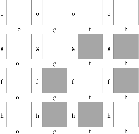
Figure 4: Distinct boundary sets in the $\hbox{\mbm Z}_{2}\times\hbox{\mbm Z}_{2}$

References

• [1] G. Aldazabal, L.E. Ibanez and F. Quevedo, JHEP 0002 (2000) 015;
G. Aldazabal, L.E. Ibanez, F. Quevedo and A. Uranga, JHEP 0102 (2001) 047;
I. Antoniadis, E. Dudas and A. Sagnotti, Phys. Lett. B464 (1999) 38;
I. Antoniadis, E. Kiritsis and N. Tomaras, Phys. Lett. B486 (2000) 186;
D. Bailin, G.V. Kraniotis and A. Love, Phys. Lett. B502 (2001) 209; Phys. Lett. B530 (2002) 202; hep-th/0210219
R. Blumenhagen, L. Goerlich, B. Kors and D. Lust, JHEP 0010 (2000) 006; Nucl. Phys. B616 (2001) 3;
R. Blumenhagen, V. Braun, B. Kors and D. Lust, JHEP 0207 (2002) 026;
Z. Kakushadze, G. Shiu, S. H. Henry Tye Nucl. Phys. B533 (1998) 25;
M. Cvetic, G. Shiu and A. Uranga, Nucl. Phys. B615 (2001) 3;
M. Cvetic. P. Langacker. G. Shiu hep-th/0206115;
L. E. Ibanez, R. Rabadan, A. M. Uranga Nucl. Phys. B542 (1999) 112; JHEP 0111 (2001) 002;
J. Ellis, P. Kanti, D. V. Nanapoulos, Nucl. Phys. B647 (2002) 235;
C. Kokorelis hep-th/0207234.
• [2] P. Horava and E. Witten, Nucl. Phys. B460 (1996) 506; Nucl. Phys. B475 (1996) 94.
• [3] R. Donagi, A. Lukas, B.A. Ovrut and D. Waldram, JHEP 9905 (1999) 018; JHEP 9906 (1999) 034;
R. Donagi, B.A. Ovrut, T. Pantev and D. Waldram, Class. Quant. Grav. 17 (2000) 1049; Adv. Theor. Math. Phys. 5 (2002) 93.
• [4] I. Antoniadis, G. D’Appollonio, E. Dudas and A. Sagnotti Nucl. Phys. B565 (2000) 123-156, hep-th/9907184.
• [5] A.E. Faraggi, R. Garavuso and J.M. Isidro, Nucl. Phys. B641 (2002) 111; hep-th/0209245; A.E. Faraggi and R.Garavuso, hep-th/0301147.
• [6] See e.g. T. Friedmann and E. Witten, hep-th/0211269, and references therein.
• [7] D.J. Gross, J.A. Harvey, J.A. Martinec and R. Rohm, Phys. Rev. Lett. 54 (1985) 502; Nucl. Phys. B256 (1986) 253.
• [8] M. Dine and N. Seiberg, Phys. Lett. B162 (1985) 299;
M. Dine and Y. Shirman, Phys. Rev. D63 (2001) 046005;
S.A. Abel and G. Servant, Nucl. Phys. B597 (2001) 3.
• [9] M. Berkooz and R.G. Leigh, Nucl. Phys. B483 (1997) 187;
R. Gopakumar and S. Mukhi, Nucl. Phys. B479 (1996) 260;
I. Antoniadis, G. D’Appollonio, E. Dudas and A. Sagnotti, Nucl. Phys. B565 (2000) 123;
J. Park, R. Rabadan and A.M. Uranga, Nucl. Phys. B570 (2000) 38;
M. Bianchi, J.F. Morales and G. Pradisi, Nucl. Phys. B573 (2000) 314;
M.R. Gaberdiel, JHEP 0011 (2000) 026.
• [10] I. Antoniadis, J.R. Ellis, J.S. Hagelin and D.V. Nanopoulos, Phys. Lett. B231 (1989) 65;
A.E. Faraggi, D.V. Nanopoulos and K. Yuan, Nucl. Phys. B335 (1990) 347;
I. Antoniadis, G.K. Leontaris, and J. Rizos, Phys. Lett. B245 (1990) 161;
A.E. Faraggi, Phys. Lett. B274 (1992) 47; Phys. Lett. B278 (1992) 131; Nucl. Phys. B387 (1992) 239; Nucl. Phys. B428 (1994) 111;
G.B. Cleaver et al, Nucl. Phys. B545 (1999) 47;
G.B. Cleaver, et al, Phys. Lett. B455 (1999) 135; Nucl. Phys. B620 (2002) 259; Phys. Rev. D63 (2001) 066001; Phys. Rev. D65 (2002) 106003; hep-ph/0301037.
• [11] I. Antoniadis, C. Bachas, and C. Kounnas, Nucl. Phys. B289 (1987) 87;
H. Kawai, D.C. Lewellen, and S.H.-H. Tye, Nucl. Phys. B288 (1987) 1.
• [12] A.E. Faraggi and D.V. Nanopoulos, Phys. Rev. D48 (1993) 3288;
A.E. Faraggi, Int. J. Mod. Phys. A14 (1999) 1663.
• [13] A.E. Faraggi, Phys. Lett. B326 (94) 62;
J. Ellis, A.E. Faraggi and D.V. Nanopoulos, Phys. Lett. B419 (1998) 123.
• [14] K. Narain, Phys. Lett. B169 (1986) 41;
K.S. Narain, M.H. Sarmadi and E. Witten, Nucl. Phys. B279 (1987) 369.
• [15] P. Berglund, J. Ellis, A.E. Faraggi, D.V. Nanopoulos and Z. Qiu, Phys. Lett. B433 (1998) 269; Int. J. Mod. Phys. A15 (2000) 1345..
• [16] C. Vafa and E. Witten, Nucl.Phys.Proc.Suppl. 46 (1996) 225;
C. Angelantonj, I. Antoniadis and K. Förger, Nucl. Phys. B555 (1999) 116.
• [17] A.E. Faraggi, Phys. Lett. B544 (2002) 207.
• [18] C. Angelantonj and A. Sagnotti, Phys. Rep. 371 (2002) 1.
• [19] I. Antoniadis, E. Dudas and A. Sagnotti, Nucl. Phys. B544 (1999) 469.
• [20] C. Angelantonj, Nucl. Phys. B566 (2000) 126.
• [21] G. Shiu and S.H. Henry Tye, Phys. Rev. D58 (1998) 086001.
• [22] A. Abouelsaood, C.G. Callan, C.R. Nappi and S.A. Yost, Nucl. Phys. B280 (1987) 599.