de Sitter Vacua in String Theory

Abstract

We outline the construction of metastable de Sitter vacua of type IIB string theory. Our starting point is highly warped IIB compactifications with nontrivial NS and RR three-form fluxes. By incorporating known corrections to the superpotential from Euclidean D-brane instantons or gaugino condensation, one can make models with all moduli fixed, yielding a supersymmetric AdS vacuum. Inclusion of a small number of ${\overline{D3}}$ branes in the resulting warped geometry allows one to uplift the AdS minimum and make it a metastable de Sitter ground state. The lifetime of our metastable de Sitter vacua is much greater than the cosmological timescale of $10^{10}$ years. We also prove, under certain conditions, that the lifetime of dS space in string theory will always be shorter than the recurrence time.

I Introduction

There has recently been a great deal of interest in finding de Sitter (dS) vacua of supergravity and string theory. This is motivated in part by the desire to construct possible models for late-time cosmology (since a small positive cosmological constant seems to be required by recent data data ), and in part by more conceptual worries that arise in the study of dS quantum gravity (as discussed, for instance, in conceptual ). The no-go theorem of maldanun guarantees that such solutions cannot be obtained in string or M-theory by using only the lowest order terms in the 10d or 11d supergravity action, but one expects that corrections to the leading order Lagrangian in the $g_{s}$ or $\alpha^{\prime}$ expansion or inclusion of extended sources (branes) should improve the situation. Indeed, a careful discussion of how such additional sources (which are present in string theory) invalidate the no-go theorem for warped backgrounds and allow one to find highly warped compactifications appears in GKP . Additional sources which violate the assumptions of the theorem were shown to yield dS vacua in ${\it noncritical}$ string theory in MSS .

Here, we use our knowledge of quantum corrections and extended objects in string theory to argue that there are dS solutions of ordinary critical string theory. Our basic strategy is to first freeze all the moduli present in the compactification, while preserving supersymmetry. We then add extra effects that break supersymmetry in a controlled way and lift the minimum of the potential to a positive value, yielding dS space. To illustrate the construction we work in the specific context of IIB string theory compactified on a Calabi-Yau (CY) manifold in the presence of flux. As described in GKP such constructions allow one to fix the complex structure moduli, but not the Kähler moduli of the compactification. In particular, to leading order in $\alpha^{\prime}$ and $g_{s}$, the Lagrangian possesses a no-scale structure which does not fix the overall volume (we shall assume that this is the ${\it only}$ Kähler modulus in the rest of this note; it is of course possible to construct explicit models which have this property). In order to achieve the first step of fixing all moduli, we therefore need to consider corrections which violate the no-scale structure. Here we focus on quantum non-perturbative corrections to the superpotential which are calculable and show that these can lead to supersymmetry preserving AdS vacua in which the volume modulus is fixed in a controlled manner.

Having frozen all moduli we then introduce supersymmetry breaking by adding a few ${\overline{D3}}$ branes in the compactification; this is a compactified version of the situation discussed in KPV . The addition of ${\overline{D3}}$ branes does not introduce additional moduli: their worldvolume scalars are frozen by a potential generated by the background fluxes KPV . Inclusion of anti-D3 branes in the absence of other corrections yields a run-away to infinite volume of the compact space (since the energy density in the ${\overline{D3}}$ branes generates a tadpole for the volume modulus). However, we show that in the presence of the quantum corrections we have described, in a sufficiently warped background the ${\overline{D3}}$ tension can be a small enough correction to lift the formerly AdS vacuum to positive cosmological constant, without destabilizing the minimum.

The extent of supersymmetry breaking and also the resulting cosmological constant of the dS minimum can be varied in our construction, within a range, in two ways. One may vary the number of ${\overline{D3}}$ branes which are introduced in the above manner, and one can also vary the warping in the compactification (by tuning the number of flux quanta through various cycles). It is important to note that this corresponds to a freedom to tune ${\it discrete}$ parameters, so while fine-tuning is possible, one should not expect to be able to tune to arbitrarily high precision. Since there is still a vacuum at very large radius with approximately zero energy (this is the Dine-Seiberg runaway vacuum dinesei ), any dS minimum is only a false vacuum; but it is only destabilized by tunneling effects, and we argue that the lifetimes one can achieve are extremely long. In addition, we argue that under the assumption that the potential between the dS minimum and the Dine-Seiberg vacuum at infinity is positive (which will be true in any simple examples, since a single dS maximum is the only intervening critical point), the lifetime of the dS minimum is ${\it always}$ shorter than the timescale for Poincaré recurrences discussed in Susskind .

While our emphasis in this paper is on dS vacua it is worth remarking that the first step of our construction, which freezes all moduli, is of interest in its own right (for another recent approach to this problem, see Acharya ; other recent ideas about fixing the volume modulus, while leaving other moduli unfixed, appear in john and references therein). In fact moduli stabilization has been an important open question in string theory and related phenomenology. We show that this can be achieved by putting together a few different effects, all of which are quite well understood by now. Preserving susy allows us to carry out this analysis with control. Once all moduli are frozen, susy breaking effects other than the introduction of ${\overline{D3}}$ branes alone can also be considered. Some of these, like the D3/D7 inflationary models of DasKal , or models with both branes and anti-branes bantib , are also of possible cosmological interest.

A more complete discussion of the possible cosmological toy models that one can construct using combinations of the ingredients described in this paper, in the spirit of KL , will appear in toappear .

We should note that there has been a great deal of interesting work on constructing dS solutions in supergravity and string theory. dS minima of 4d gauged supergravities which do not as yet have a known string theory embedding appeared in Fre ; Panda , while dS compactifications of gauged 6d supergravity appear in Quevedo . The work of MSS constructs dS vacua in supercritical string theory using many of the same ingredients which arise here. Finally, the importance of using fluxes in the cosmological context was stressed in BP , where however the problem of moduli stabilization was left as a black box (related ideas appeared in Feng ). Cosmology of the simplest flux compactifications, on the $T^{6}/Z_{2}$ orientifold DRS ; KST ; PolFrey (whose gauged supergravity description is worked out in Ferrara ), was recently investigated in Frey .

II Flux compactifications of IIB string theory, including corrections

In this section, we briefly describe the required knowledge of flux compactifications of type IIB string theory. In section IIA we describe the models of GKP , and in section IIB we enumerate various quantum corrections which can modify the superpotential and Kähler potential used in GKP . In section IIC, we show that incorporating the generic corrections can yield (supersymmetric) AdS minima with all moduli stabilized.

II.1 Calabi-Yau orientifolds with flux

We start with F-theory Vafa compactified on an elliptic CY fourfold $X$. The F-theory fourfold is a useful way of encoding the data of a solution of type IIB string theory; the base manifold $M$ of the fibration encodes the IIB geometry, while the variation of the complex structure $\tau$ of the elliptic fiber describes the profile of the IIB axio-dilaton. In such a model, one has a tadpole condition

$${\chi(X)\over 24}~{}=~{}N_{D3}+{1\over{2\kappa_{10}^{2}T_{3}}}\int_{M}H_{3}\wedge F_{3}~{}.$$ (1)

Here $T_{3}$ is the tension of a $D3$ brane, $N_{D3}$ is the net number of ($D3-{\overline{D3}}$) branes one has inserted filling the noncompact dimensions, and $H_{3}$, $F_{3}$ are the three-form fluxes in the IIB theory which arise in the NS and RR sector, respectively. As shown by Sen Sen , in the absence of flux, it is always possible to deform such an F-theory model to a locus in moduli space where it can be thought of as an orientifold of a IIB Calabi-Yau compactification. For this reason, we will use the language of IIB orientifolds, with $M$ being the Calabi-Yau threefold which is orientifolded. In this language, the term ${\chi(X)\over 24}$ counts the negative D3-brane charge coming from the $O3$ planes and the induced D3 charge on $D7$ branes, while the terms on the right-hand side count the net D3 charge from transverse branes and fluxes in the CY manifold. As in GKP , we will assume we are working with a model having only one Kähler modulus, so $h^{1,1}(M)=1$ ($h^{1,1}(X)=2$, and one modulus is frozen in taking the F-theory limit, where one shrinks the elliptic fiber). Such models can be explicitly constructed, by e.g. using the examples of CY fourfolds in fourlist or by explicitly constructing orientifolds of known CY threefolds with $h^{1,1}=1$.

In the presence of the nonzero fluxes, one generates a superpotential for the Calabi-Yau moduli, which follows from GVW (see also Taylor ; Klemm ) and is of the form

$$W~{}=~{}\int_{M}G_{3}\wedge\Omega$$ (2)

where $G_{3}=F_{3}-\tau H_{3}$, with $\tau$ the IIB axiodilaton. Combining this with the tree-level Kähler potential

$$K~{}=~{}-3\ln[-i(\rho-\bar{\rho})]-\ln[-i(\tau-\bar{\tau})]-\ln[-i\int_{M}\Omega\wedge{\overline{\Omega}}]$$ (3)

where $\rho$ is the single volume modulus ($\rho=b/\sqrt{2}+ie^{4u-\phi}$; our conventions are as in GKP ), and using the standard $N=1$ supergravity formula for the potential, one finds

$$V ~{}=~{}e^{K}\left(\sum_{a,b}g^{a\bar{b}}D_{a}W\overline{D_{b}W}-3|W|^{2}\right)\to$$ (4)

$$e^{K}(\sum_{i,j}g^{i\bar{j}}D_{i}W\overline{D_{j}W})$$

Here, $a,b$ runs over all moduli fields, while $i,j$ runs over all moduli fields except $\rho$; and we see that because $\rho$ does not appear in (2), it cancels out of the potential energy (4), leaving the positive semi-definite potential characteristic of no-scale models noscale .

One should use this potential as follows. Fix an integral choice of $H_{3},F_{3}$ in $H^{3}(M,{\bf Z})$; then, the potential (4) fixes the moduli at values where the resulting $G_{3}$ is imaginary self-dual (ISD). Supersymmetric solutions furthermore require $G_{3}$ to be type (2,1) (more generally, $G_{3}$ would have a (0,3) piece). Thus in supersymmetric solutions $W=0$ on the vacuum, while in the nonsupersymmetric solutions, $W=W_{0}$, a constant which is determined by the (0,3) piece of $G_{3}$. In generic solutions, the complex structure moduli of the F-theory fourfold (in IIB language, the complex structure moduli, the dilaton, and the moduli of D7 branes) are completely fixed, leaving only the volume modulus $\rho$. The scale of the masses $m$ for the moduli which are fixed is

$$m\sim{\alpha^{\prime}\over R^{3}}$$ (5)

where $R$ is the radius of the manifold ($\rm Im\,\rho$ scales like $R^{4}$). In this approximation, $R$ is unfixed. By tuning flux quanta, it is possible (at least in some cases) to fix $g_{s}$ at small values, though not arbitrarily small.

There is one last point we will need to use in section III. The fluxes (and any transverse branes) serve as sources for a warp factor. Therefore, such models with branes and flux are generically warped compactifications. In fact, as shown in GKP , following earlier work of Beckers ; Verlinde ; DRS ; Mayr ; Greene , it is possible to construct models with exponentially large warping. One can write the Einstein frame metric of the compactification as

$$ds_{10}^{2}~{}=~{}e^{2A(y)}\eta_{\mu\nu}dx^{\mu}dx^{\nu}+e^{-2A(y)}\tilde{g}_{mn}(y)dy^{m}dy^{n}$$ (6)

with $y$ coordinatizing the compact dimensions, and $\tilde{g}_{mn}$ the unwarped metric on $M$ (so in the orientifold limit, it is a Calabi-Yau metric). Then it is shown in GKP (by compactifying the Klebanov-Strassler solution KS ) that one can construct models parametrized by flux integers $M,K$ such that

$$e^{A_{min}}\sim\exp[-(2\pi K)/(3g_{s}M)]$$ (7)

with $e^{A}$ being of order one at generic points. This means in particular that with reasonably small flux quanta, one can generate exponentially large ratios of scales in such models.

In the following, we will assume that $g_{s}$ and the complex structure moduli have been fixed at the scale (5) by a suitable choice of flux, and concentrate on an effective field theory for the volume modulus $\rho$. This is self-consistent, in that the final mass for $\rho$ will be small compared to (5). One last comment. Light states could also arise from modes living in the throat region which experiences large warping. We assume here that any such excitations are gapped, as in KS . Then typically the $\rho$ modulus, which has a Planck scale suppressed mass, will be much lighter than these excitations and we can neglect them as well in the low energy theory.

II.2 Corrections to the no-scale models

Here, we write down two known sources of corrections to the no-scale models, both parametrize possible corrections to the superpotential (2). Then, in section IIC, we show that including either correction to the superpotential yields supersymmetric models with AdS vacua.

1) Witten has argued that in type IIB compactifications of this type, there can be corrections to the superpotential coming from Euclidean D3 branes witsup . This happens when the fourfold $X$ used for F-theory compactification admits divisors of arithmetic genus one, which project to four-cycles in the base $M$. In the presence of such instantons, there is a correction to the superpotential which at large volume yields a new term

$$W_{\rm inst}=T(z_{i})\exp(2\pi i\rho)$$ (8)

where $T(z_{i})$ is a complex structure dependent one-loop determinant, and the leading exponential dependence comes from the action of a Euclidean D3 brane wrapping a four-cycle in $M$. Since the $z_{i}$ and the dilaton are fixed by the fluxes at a scale (5), we can integrate them out and view (8) as simply providing a superpotential for the volume modulus.

2) In general models of this sort, one finds (at special loci in the complex structure moduli space) non-Abelian gauge groups arising from geometric singularities in $X$, or in type IIB language, from stacks of D7 branes wrapping 4-cycles in $M$. Assume that the fluxes have fixed one at a point in moduli space where this phenomenon occurs (examples appear in santrip , for instance). Consider a stack of $N_{c}$ coincident branes. The 4d gauge coupling of the $SU(N_{c})$ Yang-Mills theory on such wrapped branes (we ignore the decoupled $U(1)$ factor) satisfies

$${8\pi^{2}\over g_{YM}^{2}}=2\pi{R^{4}\over g_{s}}=2\pi\,{\rm Im\,\rho}~{}.$$ (9)

Since the complex structure moduli of $X$ are completely fixed, the D7 brane moduli (at least in cases where the 4-cycle being wrapped has vanishing $h^{1}$, which are easy to arrange) are also fixed. Therefore, any charged matter fields (which would create a Higgs branch for the D7 gauge theory) have also been given a mass at a high-scale; and the low-energy theory is pure $N=1$ supersymmetric $SU(N_{c})$ gauge theory. This theory undergoes gluino condensation, which results in a nonperturbative superpotential

$$W_{\rm gauge}=\Lambda_{N_{c}}^{3}=Ae^{2\pi i\rho\over N_{c}}$$ (10)

where $\Lambda_{N_{c}}$ is the dynamical scale of the gauge theory, and the coefficient $A$ is determined by the energy scale below which the the SQCD theory is valid (There are also threshold corrections in general, these contribute subleading effects.) We see that this leads to an exponential superpotential for $\rho$ similar to the one above (but with a fractional multiple of $\rho$ in the exponent, since the gaugino condensate looks like a fractional instanton effect in $W$).

So effects 1) and 2) have rather similar consequences for our analysis; we will simply assume that there is an exponential superpotential for $\rho$ at large volume. In our companion paper toappear , we investigate some interesting possibilities for cosmology if there are multiple non-Abelian gauge factors. Using the fourfolds in fourlist , it is easy to construct examples (with $h^{1,1}(X)=2$) which could yield gauge groups of total rank up to $\sim 30$. The results of kaplouis suggest that much larger ranks should be possible.

One important comment is in order before we proceed. Besides corrections to the superpotential of the kind discussed above, there are also corrections to the Kähler potential (see e.g. bbhl for a calculation of some leading corrections). In our analysis we will ensure that the volume modulus is stabilized at values which are parametrically large compared to the string scale. This makes our neglect of Kähler corrections self consistent.

II.3 Supersymmetric AdS Vacua

Here, we show that the corrections to the superpotential considered above can stabilize the volume modulus, leading to a susy preserving AdS minimum. We perform an analysis of the vacuum structure just keeping the tree-level Kähler potential

$$K=-3\ln[-i(\rho-\overline{\rho})]$$ (11)

and a superpotential

$$W=W_{0}+Ae^{ia\rho}~{}.$$ (12)

$W_{0}$ is a tree level contribution which arises from the fluxes. The exponential term arises from either of the two sources above, and the coefficient $a$ can be determined accordingly. In keeping with the fact that the complex structure moduli and the dilaton have received a mass (5), we have set them equal to their VEVs and consider only the low-energy theory of the volume modulus. To avoid the need to worry about additional open-string moduli, we assume the tadpole condition (1) has been solved by turning on only flux, i.e. with no additional $D3$ branes.

At a supersymmetric vacuum $D_{\rho}W=0$. We simplify things by setting the axion in the $\rho$ modulus to zero, and letting $\rho=i\sigma$. In addition we take $A,a$ and $W_{0}$ to be all real and $W_{0}$ negative. The minimum then lies at

$$DW=0\quad\rightarrow\quad W_{0}=-Ae^{-a\,\sigma_{cr}}(1+{2\over 3}\,a\,\sigma_{cr})$$ (13)

The potential, $V=e^{K}\left(G^{\rho\overline{\rho}}D_{\rho}W\overline{D_{\rho}W}-3|W|^{2}\right)$, at the minimum is negative and equal to

$$V_{\rm AdS}=(-3e^{K}W^{2})_{AdS}=-{a^{2}A^{2}e^{-2\,a\,\sigma_{cr}}\over 6\,\sigma_{cr}}$$ (14)

We see that we have stabilized the volume modulus while preserving supersymmetry. It is important to note that the AdS minimum is quite generic. Any corrections to the Kähler potential will still result in a susy minimum which solves (13).

A few comments are in order before we proceed. A controlled calculation requires that $\sigma\gg 1$, this ensures that the supergravity approximation is valid and the $\alpha^{\prime}$ corrections to the Kähler potential are under control. It also requires that $a\,\sigma>1$ so that the contribution to the superpotential from a single (fractional) instanton is reliable. Generically, if the fluxes break supersymmetry, $W_{0}\sim O(1)$, and these conditions will not be met. However it is reasonable to expect that by tuning fluxes one can arrange so that $W_{0}\ll 1$. In these circumstances we see from (13) that $a\,\sigma>1$. Taking $a<1$, one can then ensure that $\sigma\gg 1$, as required.

As an illustrative example we consider $W_{0}=-10^{-4}$, $A=1$, $a=0.1$. This results in a minimum at $\sigma_{cr}\sim 113$.

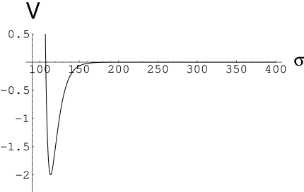
Figure 1: Potential (multiplied by $10^{15}$) for the case of exponential superpotential with $W_{0}=-10^{-4}$, $A=1$, $a=0.1$. There is an AdS minimum.

Another possibility to get a minimum at large volume is to consider a situation where the fluxes preserve susy, and the superpotential involves multiple exponential terms, i.e. “racetrack potentials” for the stabilization of $\rho$ racetrack . Such a superpotential could arise from multiple stacks of seven branes wrapping four cycles which cannot be deformed into each other in a susy preserving manner toappear . In this case by tuning the ranks of the gauge groups appropriately one can obtain a parametrically large value of $\sigma$ at the minimum.

Finally it is plausible that in some cases, there could be some other moduli which have not yet been fixed in this approximation (if, for instance, the fluxes were nongeneric and left some of the complex structure moduli of the Calabi-Yau manifold unfixed). Since the dilaton is already fixed by fluxes and the radial modulus is fixed due to non-perturbative exponential terms in the superpotential, one might find interesting and realistic cosmology driven by these other scalar fields from the compactified string theory. Here, however, we will neglect this possibility, and focus instead on another mechanism for uplifting the AdS vacuum to a dS vacuum.

III Constructing dS vacua

In this section, we uplift the supersymmetric AdS vacua of section IIC to yield dS vacua of string theory. In section IIIA, we describe the new ingredient: ${\overline{D3}}$ branes transverse to $M$. In section IIIB, we show that for reasonable choices of parameters, the inclusion of ${\overline{D3}}$ branes yields dS vacua.

III.1 $\overline{D3}$ branes in ISD fluxes

In the tadpole condition (1), there is a contribution from both localized $D3$ branes and from fluxes. To find AdS vacua with no moduli in the previous section, we assumed that the condition was saturated by turning on fluxes in the compact manifold. Now, we assume that in fact we turn on ${\it too~{}much}$ flux, so that (1) can only be satisfied by introducing one ${\overline{D3}}$ brane. In the flux background determining a solution of the sort described in section II, the $\overline{D3}$ does not have translational moduli; they are fixed by the ISD fluxes, which generate a potential for the worldvolume scalars. This kind of situation was studied in KPV .

Now, the tadpole is cancelled, but there is an extra bit of energy density from the “extra” flux and ${\overline{D3}}$ brane. In fact, as in equation (73) of KPV , one finds that the ${\overline{D3}}$ brane adds an additional energy:

$$\delta V=2{a_{0}^{4}T_{3}\over g_{s}^{4}}{1\over({\rm Im\,\rho})^{3}}$$ (15)

with $a_{0}$ the warp factor at the location of the ${\overline{D3}}$ brane. As described in KPV , in the presence of ISD fluxes of the sort characterizing the Klebanov-Strassler throat, any anti-D3 branes are driven to the end of the throat, where the warp factor is minimized. It follows from (7) that the value of $a_{0}$ is exponentially small, and hence in suitable models the inclusion of a ${\overline{D3}}$ adds to the potential an exponentially suppressed term. The prefactor of $2$ in (15) arises because the ambient five-form flux adds a repulsive energy equal to the tension for an ${\overline{D3}}$ brane, see maldnast (above equation (3.9)). Note also that we are considering solutions which meet the ISD condition, even in the presence of the additional flux required to insert the ${\overline{D3}}$ brane. There are corrections to (15) but these are quadratic in the number of ${\overline{D3}}$ that are added and are small.

The important point is that due to the warping the addition of the ${\overline{D3}}$ brane breaks supersymmetry by a very small amount. In general terms, we get a term in the potential which goes like

$$\delta V={8D\over(\rm Im\,\rho)^{3}}$$ (16)

(the factor of ${\rm 8}$ is added for later convenience). The coefficient $D$ depends on the number of ${\overline{D3}}$ branes and on the warp factor at the end of the throat. These parameters can be altered by discretely changing the total flux, and the fluxes which enter in (7), respectively. This allows us to vary the coefficient $D$ and the susy breaking in the system, while still keeping them small (More properly, since the flux can only be discretely tuned, $D$ can be varied but not with arbitrary precision). We will see that by tuning the choice of $D$ one can perturb the AdS vacua of IIC to produce dS vacua with a tunable cosmological constant. The vacua will clearly only be metastable, since all of the sources of energy we have introduced vanish as $\rm Im\,\rho\to\infty$.

III.2 Uplifting AdS vacua to dS vacua

We now add to the potential a term of the form $D/\sigma^{3}$, as explained above. For suitable choices of $D$, the AdS minimum will become a dS minimum, but the rest of the potential does not change too much. There is one new important feature, however: there is a dS maximum separating the dS minimum from the vanishing potential at infinity. The potential is:

$${V~{}=~{}{aAe^{-a\sigma}\over{2\sigma^{2}}}\left({1\over 3}\sigma aAe^{-a\sigma}+W_{0}+Ae^{-a\sigma}\right)}+{D\over\sigma^{3}}$$

By fine-tuning $D$, it is easy to have the dS minimum very close to zero. For the model $W_{0}=-10^{-4}$, $A=1$, $a=0.1$ $D=3\times 10^{-9}$ we find the potential (multiplied by $10^{15}$):

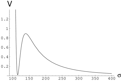
Figure 2: Potential (multiplied by $10^{15}$) for the case of exponential superpotential and including a $D\over\sigma^{3}$ correction with $D=3\times 10^{-9}$ which uplifts the AdS minimum to a dS minimum.

Note, if one does not require the minimum to be so close to zero, $D$ does not have to be fine-tuned so precisely. A dS minimum is obtained as long as $D$ lies within a range, eventually disappearing for large enough D. If one does fine tune to get the minimum very close to zero, the resulting potentials are quite steep around the dS minimum. In this circumstance, the new term basically uplifts the potential without changing the shape too much around the minimum, so the $\rho$ field acquires a surprisingly large mass (relative to the final value of the cosmological constant).

It is important to mention that the value of the volume modulus shifts only slightly in going from the AdS minimum to the new dS minimum. This means if the volume was large in the AdS minimum to begin with, it will continue to be large in the new dS minimum, guaranteeing that our approximations are valid.

If one wants to use this potential to describe the present stage of acceleration of the universe, one needs to fine-tune the value of the potential in dS minimum to be $V_{0}\sim 10^{-120}$ in units of Planck density. In principle, one could achieve it, e.g., by fine tuning $D$. However, the tuning we can really do by varying the fluxes etc. in the microscopic string theory is limited, though it may be possible to tune quite well if there are enough three-cycles in $M$.

IV How stable is the dS vacuum?

The radial modulus $\sigma=\rm Im\,\rho$ has a kinetic term ${3\over 4\sigma^{2}}(\partial\sigma)^{2}$ which follows from the Kähler potential (3). For cosmological purposes it is convenient to switch to the canonical variable $\varphi=\sqrt{3\over 2}\ln\sigma=\sqrt{3\over 2}\ln(\rm Im\,\rho)$, which has a kinetic term ${1\over 2}(\partial\varphi)^{2}$. In what follows we will use the field $\varphi$ and it should not be confused with the dilaton, $\phi$.

IV.1 General theory

The dS vacuum state $\varphi_{0}$ corresponding to the local minimum of the potential with $V_{0}>0$ is metastable. Therefore it may decay, and then the universe will roll towards large values of the field $\varphi$ and decompactify. Here we would like to address two important questions:

1) Do our dS vacua survive for a large number of Planck times? For instance, if we fine tune to get a small cosmological constant, is the dS vacuum sufficiently stable to survive during the $10^{10}$ years of the cosmological evolution? If the answer is positive, one can use the dS minimum for the phenomenological description of the current stage of acceleration (late-time inflation) of the universe.

2) Is the typical decay time of the dS vacuum longer or shorter than the recurrence time $t_{r}\sim e^{\bf S_{0}}$, where ${\bf S_{0}}={24\pi^{2}\over V_{0}}$ is the dS entropy Gibbons:1976ue ? If the decay time is longer than $t_{r}\sim e^{\bf S_{0}}$, one may need to address the issues about the consistency of the stringy description of dS space raised in conceptual ; MSS ; Susskind .

We will argue that the lifetime of the dS vacuum in our models is not too short and not too long: it is extremely large in Planck times (in particular, one can easily make models which live longer than the cosmological timescale $\sim 10^{10}$ years), and it is much shorter than the recurrence time $t_{r}\sim e^{\bf S_{0}}$.

In order to analyse this issue we will remember, following Coleman and De Luccia Coleman:1980aw , basic features of the tunneling theory taking into account gravitational effects.

To describe tunneling from a local minimum at $\varphi=\varphi_{0}$ one should consider an $O(4)$-invariant Euclidean spacetime with the metric

$$ds^{2}=d\tau^{2}+b^{2}(\tau)(d\psi^{2}+\sin^{2}\psi\,d\Omega_{2}^{2})\ .$$ (17)

The scalar field $\varphi$ and the Euclidean scale factor (three-sphere radius) $b(\tau)$ obey the equations of motion

$$\varphi^{\prime\prime}+3{b^{\prime}\over b}\varphi^{\prime}=V_{,\varphi},~{}~{}~{}~{}~{}b^{\prime\prime}=-{b\over 3}(\varphi^{\prime 2}+V)\ ,$$ (18)

where primes denote derivatives with respect to $\tau$. (We use the system of units $M_{p}=1$.)

These equations have several instanton solutions $(\varphi(\tau),\,b(\tau))$. The simplest of them are the $O(5)$ invariant four-spheres one obtains when the field $\varphi$ sits at one of the extrema of its potential, and $b(\tau)=H^{-1}\sin H\tau$. Here $H^{2}={V\over 3}$, and $V(\varphi)$ corresponds to one of the extrema. In our case, there are two trivial solutions of this type. One of them describes time-independent field corresponding to the minimum of the effective potential at $\varphi=\varphi_{0}$, with $V_{0}=V(\varphi_{0})$. Another one is related to the maximum of the potential at $\varphi=\varphi_{1}$, with $V_{1}=V(\varphi_{1})$.

Coleman-De Luccia (CDL) instantons are more complicated. They describe the field $\varphi(\tau)$ beginning in a vicinity of the false vacuum $\varphi_{0}$ at $\tau=0$, and reaching some constant value $\varphi_{f}>\varphi_{1}$ at $\tau=\tau_{f}$, where $b(\tau_{f})=0$. It is tempting to interpret CDL instantons as the tunneling trajectories interpolating between the different vacua of the theory. However, one should be careful with this interpretation because the trajectories $\varphi(\tau)$ for CDL instantons do not begin exactly in the metastable minimum $\varphi_{0}$ and do not end exactly in the absolute minimum of the effective potential. We will discuss this issue later.

According to Coleman:1980aw , the tunneling probability is given by

$$P(\varphi)=e^{-S(\varphi)+S_{0}},$$ (19)

where $S(\varphi)$ is the Euclidean action for the tunneling trajectory $(\varphi(\tau),\,b(\tau))$, and $S_{0}=S(\varphi_{0})$ is the Euclidean action for the initial configuration $\varphi=\varphi_{0}$. Note that $S(\varphi)$ in Eq. (19) for the tunneling probability is the integral over the whole instanton solution, rather that the integral over its half providing the tunneling amplitude.

The tunneling action is given by

$$S(\varphi)=\int d^{4}x\sqrt{g}\left(-{1\over 2}R+{1\over 2}(\partial\varphi)^{2}+V(\varphi)\right).$$ (20)

In $d=4$ the trace of the Einstein equation is $R=(\partial\varphi)^{2}+4V(\varphi)$. Therefore the total action can be represented by an integral of $V(\varphi)$:

$$S(\varphi)=-\int d^{4}x\sqrt{g}V(\varphi)=-{2\pi^{2}\int_{0}^{\tau_{f}}d\tau\,b^{3}(\tau)\,V(\varphi(\tau))}\ .$$ (21)

The Euclidean action calculated for the false vacuum dS solution $\varphi=\varphi_{0}$ is given by

$$S_{0}=-{24\pi^{2}\over V_{0}}<0\ .$$ (22)

Similarly, for the dS maximum $\varphi=\varphi_{1}$ one has $S_{1}=-{24\pi^{2}\over V_{1}}$.

This action for dS space $S_{0}$ has a simple sign-reversal relation to the entropy of de Sitter space ${\bf S_{0}}$:

$${\bf S_{0}}=-S_{0}=+{24\pi^{2}\over V_{0}}\ .$$ (23)

Therefore the decay time of the metastable dS vacuum $t_{\rm decay}\sim P^{-1}(\varphi)$ can be represented in the following way:

$$t_{\rm decay}=e^{S(\varphi)+\bf S_{0}}=t_{r}\ e^{S(\varphi)}\ .$$ (24)

The semiclassical approximation is applicable only for $|S(\varphi)|\gg 1$. Eq. (21) implies that for the tunneling through the barrier with $V(\varphi)>0$ (which is the case for the tunneling from dS space to Minkowski space in our model) the action $S(\varphi)$ is always negative, $S(\varphi)<0$. This means that the decay time of dS space to Minkowski space is exponentially smaller than the recurrence time $t_{r}$. The existence of the runaway vacuum at $\infty$ in field space with zero energy is a standard feature of all string theories dinesei . We conclude that the problems related to the decay time exceeding the recurrence time $t_{r}$ conceptual ; MSS ; Susskind will not appear in the simplest string theory models, where a single dS maximum will separate the dS minimum from $\infty$.

Now that we found the upper bound on the tunneling time, we will try to estimate the tunneling time in our model using some particular instanton solutions. In general, it is very difficult to find analytical solutions for the CDL instantons and calculate the tunneling probability. We will investigate this problem using two different approaches, which are, in a certain sense, opposite to each other: the thin-wall approximation and the no-wall approximation.

IV.2 Thin-wall approximation

Let us assume that one can describe the present stage of the acceleration of the universe by our model, so that $V_{0}\sim 10^{-120}$ in Planck units (more generally, the analysis of this section will work for $V_{0}$ very small compared to the starting AdS cosmological constant, which can be arranged by tuning). This is a hundred orders of magnitude smaller than the height of the barrier $V_{1}$ in our model. In Minkowski space, the condition $V_{0}\ll V_{1}$ usually means that the thin-wall approximation is applicable. Let us check whether one can use it in our case.

In application to our scenario (tunneling from dS space with vacuum energy $V_{0}>0$ to Minkowski space) one can represent the results of Coleman:1980aw in the following useful form:

$$P=\exp\left({-{{\bf S}(\varphi_{0})\over(1+(4V_{0}/3T^{2}))^{2}}}\right)\ .$$ (25)

Here $T$ is not temperature but tension of the bubble wall; in our case

$$T=\int_{\varphi_{0}}^{\infty}d\varphi\,\sqrt{2V(\varphi)}\ .$$ (26)

Eq. (25) confirms our general conclusion that the suppression of the tunneling is always smaller than $e^{-{{\bf S}(\varphi_{0})}}$, and the decay time is shorter than $t_{r}$.

There are two limiting cases of special interest: $V_{0}\gg T^{2}$ and $V_{0}\ll T^{2}$. The meaning of these two conditions becomes clear if we restore $M_{p}$ in these inequalities: $V_{0}M_{p}^{2}\gg T^{2}$ and $V_{0}M_{p}^{2}\ll T^{2}$. If we turn off the gravitational interactions ($M_{p}\to\infty$), one has $V_{0}M_{p}^{2}\gg T^{2}$, and we obtain the well known result for the tunneling in the thin-wall approximation in Minkowski space:

$$P=\exp\left({-{27\pi^{2}T^{4}\over 2V_{0}^{3}}}\right)\ .$$ (27)

From Eq. (26) one finds that $T\sim\Delta\varphi\sqrt{V_{1}}$, where $\Delta\varphi$ is the typical width of dS maximum. This means that $V_{0}\gg T^{2}$ (in units $M_{p}=1$), and one can ignore the gravitational effects in the thin-wall approximation only if

$${\Delta\phi}\ll\sqrt{V_{0}\over V_{1}}\ .$$ (28)

One can easily check that for our model this condition is not satisfied, so we must take gravitational effects into account and study an opposite limit $V_{0}\ll T^{2}$. Then in the first approximation one simply has

$$P\approx\exp\left({-{{\bf S}(\varphi_{0})}}\right)=\exp\left(-{24\pi^{2}\over V_{0}}\right)\sim\exp\left(-{10^{122}}\right)\ .$$ (29)

Thus, for all practical purposes our dS vacuum is completely stable.

On the other hand, if one expands Eq. (25) in powers of $V_{0}/T^{2}$, one finds

$$P\approx\exp\left({-{{\bf S}(\varphi_{0})}}\right)\times\exp\left({64\pi^{2}\over T^{2}}\right)\ .$$ (30)

For the sub-Planckian tension $T\ll 1$ one finds that the probability of the tunneling is exponentially larger than $P\approx\exp\left({-{{\bf S}(\varphi_{0})}}\right)$. The decay time of dS space due to CDL instantons $t^{\rm CDL}_{\rm decay}$ is much smaller than the recurrence time $t_{r}\sim\exp\left({-{{\bf S}(\varphi_{0})}}\right)$, in agreement with our general result:

$$t^{\rm CDL}_{\rm decay}\sim t_{r}\exp\left(-{64\pi^{2}\over T^{2}}\right)\ .$$ (31)

In the thin-wall approximation (for $V_{0}\ll T^{2}$) the radius of the bubble is $R_{B}=4/T$ Coleman:1980aw , whereas the thickness of the wall is approximately $\Delta R_{B}=T/V_{1}$. This means that the thin-wall approximation taking gravity into account is valid if $\Delta R_{B}\ll R_{B}$, i.e. $T^{2}\ll V_{1}$.

IV.3 “No-wall” approximation: Hawking-Moss instanton and stochastic approach to tunneling

Now we will return to the simplest instanton solutions, sitting at the dS minimum $\varphi=\varphi_{0}$ and the dS maximum $\varphi=\varphi_{1}$. According to Hawking and Moss (HM) Hawking:1981fz , they describe tunneling through the barrier, with the probability of tunneling suppressed as

$$P=e^{-S(\varphi_{1})+S(\varphi_{0}))}=\exp\left(-{24\pi^{2}\over V_{0}}+{24\pi^{2}\over V_{1}}\right)\ .$$ (32)

This result may seem rather controversial because the instanton solution $\varphi(\tau)=\varphi_{1}$ does not interpolate between the stable vacuum and the false vacuum.

In fact, as we already mentioned, the last problem appears for all CDL solutions as well. These solutions never begin exactly in the false vacuum, so how could they be considered interpolating solutions? This problem disappears in the thin-wall limit, but it shows up very clearly in numerical calculations going beyond the thin wall approximation.

There are several different ways in which one can address this issue. In GL it was noticed that instead of considering an exactly constant solution $\varphi=\varphi_{1}$ one may consider a configuration that coincides with this solution everywhere except a small vicinity of the endpoint at $\tau_{f}=\pi H^{-1}$. The action involves integration $\int d\tau\,b^{3}(\tau)L(g_{\mu\nu},\varphi)$. Since the scale factor $b(\tau)=H^{-1}\sin H\tau$ vanishes at $\tau_{f}=\pi H^{-1}$, one can make very strong modifications of the solution $\varphi=\varphi_{1}$ in a small vicinity of $\tau_{f}$ without changing the action in a significant way. If the action changes by less than $O(1)$, then each such configuration can be used for the description of tunneling despite the fact that it is not a true solution of classical equations of motion near $\tau_{f}$. This allows one to bend the solution $\varphi=\varphi_{1}$ (or the CDL solution) in such a way that it begins to interpolate between the different vacua.

One may also patch HM instantons and CDL instantons to each other in several different ways, which may provide their alternative interpretation and justify the results obtained by using CDL and HM instantons, see e.g. Linde:1998gs ; Bousso:1998vz ; Bousso:1998ed . More recently a possible interpretation of CDL and HM instantons was suggested in Banks:2002nm . Significant progress was achieved by Gen and Sasaki in the development of a consistent Hamiltonian approach to tunneling with gravity Gen:1999gi .

But these methods do not address another problem with the Hawking-Moss tunneling: Since the instanton $\varphi=\varphi_{1}$ is exactly homogeneous, it seems to describe a homogeneous tunneling in the whole universe, which is impossible. One can circumvent this problem by claiming that the whole universe is reduced to the interior of a single causal patch of size $H^{-1}$. However, this approach, which is often used for the description of eternal dS space (which does not decay), may be less useful in applications to inflationary cosmology since it loses information about the whole universe except for a small part of size $H^{-1}$.

The most intuitively transparent description of the (nearly) homogeneous tunneling was provided in Starobinsky:fx ; book ; Hardart ; LLM in the context of the stochastic approach to inflation.

One may consider quantum fluctuations of a light scalar field $\varphi$ with $m^{2}=V^{\prime\prime}\ll H^{2}=V/3$. During each time interval $\delta t=H^{-1}$ this scalar field experiences quantum jumps with the wavelength $\sim H^{-1}$ and with a typical amplitude $\delta\varphi=H/2\pi$. Then the wavelength of these fluctuations grows exponentially. As a result, quantum fluctuations lead to a local change of the amplitude of the field $\varphi$ which looks homogeneous on the horizon scale $H^{-1}$. From the point of view of a local observer, this process looks like a Brownian motion of the homogeneous scalar field. If the potential has a dS minimum at $\varphi_{0}$ with $m\ll H$, then eventually the probability distribution to find the field with the value $\varphi$ becomes time-independent: Starobinsky:fx ; book ; Hardart ; LLM

$$P(\varphi,\varphi_{0})\sim\exp\left({24\pi^{2}\over V(\varphi)}\right)\cdot\,\exp\left(-{24\pi^{2}\over V(\varphi_{0})}\right)\ .$$ (33)

This result was obtained without any considerations based on the Euclidean approach to quantum gravity. It provides a simple interpretation of the Hawking-Moss tunneling. During inflation, long wavelength perturbations of the scalar field freeze on top of each other and form complicated configurations, which, however, look almost homogeneous on the horizon scale $H^{-1}$. If originally the whole universe was in a state $\varphi_{0}$, the scalar field starts wandering around, and eventually it reaches the local maximum of the effective potential at $\varphi=\varphi_{1}$. According to (33), the probability of this event is suppressed by $\exp\left(-{24\pi^{2}\over V_{0}}+{24\pi^{2}\over V_{1}}\right)$. As soon as the field $\varphi$ reaches the top of the effective potential, it may fall down to another minimum, because it looks nearly homogeneous on a scale of horizon, and gradients of the field $\varphi$ are not strong enough to pull it back to $\varphi_{0}$. The probability of this process is given by the Hawking-Moss expression (32). However, this is not a homogeneous tunneling all over the universe, but rather a Brownian motion, which looks homogeneous on the scale $H^{-1}$ book .

One can take a logarithm of the probability distribution (33) and find that the entropy of the state with the field stochastically moving in the potential $V(\varphi)$ is given by

$${\bf S(\varphi)}={24\pi^{2}\over V(\varphi)}\ .$$ (34)

This is the simplest derivation of dS entropy that does not involve ambiguous Euclidean calculations. It is valid even for the states outside the dS minimum, as long as the condition $|m^{2}|\ll H^{2}$ (i.e. $|V^{\prime\prime}|\ll V$) remains valid.

This result allows one to obtain a simple interpretation of the HM tunneling, proposed in Linde:1998gs . Indeed, Eq. (32) has the standard thermodynamic form describing the probability of thermal fluctuations

$$P=e^{\bf\Delta S}=e^{\bf S(\varphi_{1})-\bf S(\varphi_{0})}\ .$$ (35)

A similar thermodynamic approach was recently developed in a series of papers by Susskind et al Susskind .

Since the entropy $S(\varphi_{1})=24\pi^{2}/V_{1}$ is positive, one finds another confirmation of our general result:

$$t^{\rm HM}_{\rm decay}=e^{-\bf S_{1}+\bf S_{0}}=t_{r}\ \exp\left(-{24\pi^{2}\over V_{1}}\right)\ll t_{r}\ .$$ (36)

On the other hand, in our case $S_{1}\ll S_{0}$, so in the first approximation one finds, as before, that $t^{\rm HM}_{\rm decay}\approx t_{r}\sim e^{10^{122}}$.

Note that the quasi-homogeneous HM tunneling and the CDL tunneling correspond to two different processes; depending on the potential, one of these processes may happen much faster than another. Let us compare the rate of the quasi-homogeneous HM tunneling with the rate of tunneling due to CDL instantons in the thin wall approximation for $T\ll 1$:

$${t^{\rm HM}_{\rm decay}\over t^{\rm CDL}_{\rm decay}}=\exp\left[8\pi^{2}\left({8\over T^{2}}-{3\over V_{1}}\right)\right]\ .$$ (37)

This shows that $t^{\rm HM}_{\rm decay}<t^{\rm CDL}_{\rm decay}$ (HM tunneling dominates) for $3T^{2}>8V_{1}$. Meanwhile, in the opposite case, $3T^{2}<8V_{1}$, the tunneling occurs due to CDL instantons. This is consistent with our estimate of validity of the thin wall approximation, $T^{2}\ll V_{1}$.

It is useful to represent this result in a different way. Let us use the estimate $T\sim\Delta\varphi\sqrt{V_{1}}$, where $\Delta\varphi$ is the typical width of dS maximum. This estimate implies that $3T^{2}>8V_{1}$ and $t^{\rm HM}_{\rm decay}<t^{\rm CDL}_{\rm decay}$ if $\Delta\varphi>1$, i.e. if the width of the maximum is much greater than the Planck mass. For the potentials with the nearly Minkowski minima this condition coincides with the inflationary slow-roll condition $|V^{\prime\prime}|<V$.

Thus we are coming to the conclusion that the HM tunneling, and the thermodynamic approach discussed above, are most efficient for the description of the tunneling in the inflationary universe, where their validity has been firmly established by the stochastic approach to inflation. On the other hand, in the situations where the potentials are very thin, $\Delta\phi\ll 1$, one should use the CDL instantons, and the thin-wall approximation is valid.

This result has a very simple interpretation. CDL instantons describe tunneling through the barrier. Meanwhile, HM instantons in the inflationary regime can be interpreted in terms of the Brownian motion, when the field slowly climbs to the top of the barrier due to accumulation of quantum fluctuations with the Hawking temperature $H/2\pi$. If the barrier is very wide, it is easier to climb the barrier rather that to tunnel through it. In this case the HM tunneling prevails and the stochastic/thermodynamic description of this process in terms of dS entropy is very useful. If the barrier is very thin, it is easier to tunnel, and CDL instantons are more efficient.

For the simple models with the parameters given in our paper one has $3T^{2}<8V_{1}$, and the tunneling occurs mainly due to CDL instantons. Even in this case the stochastic/thermodynamic approach may remain useful: If this approach is valid not only in the context of inflationary cosmology with $|V^{\prime\prime}|\ll V$ but also in the situations with $|V^{\prime\prime}|\gtrsim V$, it provides a simple upper bound on the decay time of dS space, $t_{\rm decay}<e^{\bf S(\varphi_{0})-\bf S(\varphi_{1})}$.

V Discussion

It has been a difficult problem to construct realistic cosmologies from string theory, as long as the moduli fields are not frozen. In this note, we have seen that it is possible to stabilize all moduli in a controlled manner in the general setting of compactifications with flux. This opens up a promising arena for the construction of string cosmologies.

More specifically, we have seen that it should be possible to construct metastable dS vacua in the general framework of GKP , by including anti-branes KPV and incorporating non-perturbative corrections to the superpotential from D3 instantons witsup or low-energy gauge dynamics. For cosmology, it might be more interesting to include a more complicated sector at the end of the warped throat. For instance, the D3/D7 inflationary models of DasKal , or models with both branes and anti-branes bantib , could be of interest in this context. It should also be possible to make similar constructions in the heterotic theory, perhaps using the models of bbdg as a starting point (and then incorporating a mechanism to stabilize the dilaton in a controlled manner).

It is worth summarizing why we believe the constructions in this paper are reliable. Our analysis was carried out in the framework of supergravity. There are two kinds of corrections to this analysis, in the $g_{s}$ and $\alpha^{\prime}$ expansions. By tuning the fluxes we have argued that both of these can be controlled. For example, it is reasonable to believe that $g_{s}$ can be stabilized at a value of order $g_{s}\sim 0.1$ and the volume $\sigma\gg 1$ (for the volume this was discussed in section II C). Note that for reliability we do not require that the dilaton and volume be made arbitrarily small or big; in fact this is not possible since the fluxes can only be tuned discretely. We only require that these moduli take appropriately small or big values, and this can be achieved, especially if $M$ has enough three-cycles, yielding many possible choices of flux background.

We were also able to prove, in section IV, that our dS minima are short lived compared to the timescale for Poincaré recurrences. This generalizes to any construction where the dS minimum is separated from the Dine-Seiberg run-away vacuum (which is ubiquitous in string theory) by a potential which remains non-negative; the simplest controlled examples in string theory will have this feature. One can also imagine more complicated shapes of the potential between the dS minimum and infinity, which include some intervening AdS critical points. It is natural to wonder if a more general statement can be obtained that would apply in these cases as well.

Finally, it would be interesting to discover string theory models which naturally incorporate both $>60$ e-foldings of early universe inflation, and a late-time cosmology in agreement with the most recent data data . (To show that it is possible to obtain a small enough value of the dS cosmological constant for late-time cosmology, one would have to demonstrate that an idea along the lines of BP can be implemented in this context.) Some further steps towards making more realistic cosmological toy-models inspired by string theory, in the same general framework as this note, will be presented in toappear .

It is a pleasure to thank I. Bena, A. Dabholkar, M. Dine, S. Gukov, M. Headrick, S. Hellerman, L. Kofman, A. Maloney, A. Sen, E. Silverstein, A. Strominger, L. Susskind, P. Tripathi, and H. Verlinde for useful discussions. This work was supported in part by NSF grant PHY-9870115. The work by A.L. was also supported by the Templeton Foundation grant No. 938-COS273. The work of S.K. was also supported by a David and Lucile Packard Foundation Fellowship for Science and Engineering, NSF grant PHY-0097915 and the DOE under contract DE-AC03-76SF00515. S.P.T. acknowledges the support of the DAE, the Swarnajayanti Fellowship, and most of all the people of India.

References

- (1) S. Perlmutter et al. [Supernova Cosmology Project Collaboration], “Measurements of Omega and Lambda from 42 High-Redshift Supernovae,” Astrophys. J. 517, 565 (1999) [astro-ph/9812133]; A. G. Riess et al. [Supernova Search Team Collaboration], “Observational Evidence from Supernovae for an Accelerating Universe and a Cosmological Constant,” Astron. J. 116, 1009 (1998) [astro-ph/9805201].
- (2) T. Banks, “Cosmological Breaking of Supersymmetry? Or Little Lambda goes back to the future 2,” [arXiv:hep-th/0007146]; S. Hellerman, N. Kaloper and L. Susskind, “String theory and quintessence,” JHEP 0106, 003 (2001) [arXiv:hep-th/0104180]; W. Fischler, A. Kashani-Poor, R. McNees and S. Paban, “The acceleration of the Universe: A challenge for string theory,” [arXiv:hep-th/0104181]; E. Witten, “Quantum Gravity in de Sitter Space,” [arXiv:hep-th/0106109]; A. Strominger, “The dS/CFT Correspondence,” JHEP 0110, 034 (2001) [hep-th/0106113].
- (3) J. Maldacena and C. Nunez, “Supergravity Description of Field Theories on Curved Manifolds and a No Go Theorem,” Int. J. Mod. Phys. A16, 822 (2001), [arXiv:hep-th/0007018]; G.W. Gibbons, “Aspects of Supergravity Theories,” in , eds. F. del Aguila, J.A. de Azcarraga and L.E. Ibanez (World Scientific 1985) pp.346-351; B. de Wit, D.J. Smit and N.D. Hari Dass, “Residual Supersymmetry of Compactified Supergravity,” Nucl. Phys. B283, 165 (1987).
- (4) S. B. Giddings, S. Kachru and J. Polchinski, “Hierarchies from fluxes in string compactifications,” Phys. Rev. D66, 106006 (2002) [arXiv:hep-th/0105097].
- (5) E. Silverstein, “(A)dS Backgrounds from Asymmetric Orientifolds,” [arXiv:hep-th/0106209]; A. Maloney, E. Silverstein and A. Strominger, “de Sitter Space in Noncritical String Theory,” [arXiv:hep-th/0205316].
- (6) S. Kachru, J. Pearson and H. Verlinde, “Brane/Flux Annihilation and the String Dual of a Non-Supersymmetric Field Theory,” JHEP 0206, 021 (2002) [arXiv:hep-th/0112197].
- (7) M. Dine and N. Seiberg, “Is the superstring weakly coupled?,” Phys. Lett. B162, 299 (1985).
- (8) L. Dyson, J. Lindesay and L. Susskind, “Is there really a de Sitter/CFT duality,” JHEP 0208, 045 (2002) [arXiv:hep-th/0202163]; L. Dyson, M. Kleban and L. Susskind, “Disturbing implications of a cosmological constant,” JHEP 0210, 011 (2002) [arXiv:hep-th/0208013]; N. Goheer, M. Kleban and L. Susskind, “The trouble with de Sitter space,” arXiv:hep-th/0212209.
- (9) B.S. Acharya, “A Moduli Fixing Mechanism in M-theory,” [arXiv:hep-th/0212294].
- (10) S. Hellerman, J. McGreevy and B. Williams, “Geometric Constructions of Non-geometric String Theories,” [arXiv:hep-th/0208174]; A. Dabholkar and C. Hull, “Duality Twists, Orbifolds and Fluxes,” [arXiv:hep-th/0210209].
- (11) K. Dasgupta, C. Herdeiro, S. Hirano and R. Kallosh, “D3/D7 Inflationary Model and M-theory,” Phys. Rev. D65, 126002 (2002) [arXiv:hep-th/0203019].
- (12) S. Alexander, “Inflation from D/Anti-D Brane Annihilation,” Phys. Rev. D65, 23507 (2002) [arXiv:hep-th/0105032]; G. Dvali, Q. Shafi and S. Solganik, “D-Brane Inflation,” [arXiv:hep-th/0105203]; C.P. Burgess, M. Majumdar, D. Nolte, F. Quevedo, G. Rajesh and R. Zhang, “The Inflationary Brane Anti-Brane Universe,” JHEP 0107, 047 (2001) [arXiv:hep-th/0105204].
- (13) R. Kallosh, A. Linde, S. Prokushkin and M. Shmakova, “Supergravity, Dark Energy and the Fate of the Universe,” [arXiv:hep-th/0208156].
- (14) S. Kachru, R. Kallosh, A. Linde and S. P. Trivedi, in preparation.
- (15) P. Fre, M. Trigiante and A. Van Proeyen, “Stable de Sitter Vacua from Supergravity,” [arXiv:hep-th/0205119].
- (16) M. de Roo, D.B. Westra and S. Panda, “de Sitter solutions in matter coupled supergravity,” [arXiv:hep-th/0212216].
- (17) Y. Aghababaie, C.P. Burgess, S.L. Parameswaran and F. Quevedo, “SUSY Breaking and Moduli Stabilization from Fluxes in Gauged 6d Supergravity,” [arXiv:hep-th/0212091].
- (18) R. Bousso and J. Polchinski, “Quantization of Four-Form Fluxes and Dynamical Neutralization of the Cosmological Constant,” JHEP 0006, 006 (2000), [arXiv:hep-th/0004134].
- (19) J. Feng, J. March-Russell, S. Sethi and F. Wilczek, “Saltatory Relaxation of the Cosmological Constant,” Nucl. Phys. 602, 307 (2001) [arXiv:hep-th/0005276].
- (20) K. Dasgupta, G. Rajesh and S. Sethi, “M-theory, Orientifolds and G-Flux,” JHEP 9908, 023 (1999), [arXiv:hep-th/9908088].
- (21) S. Kachru, M. Schulz and S. P. Trivedi, “Moduli Stabilization from Fluxes in a Simple IIB Orientifold,” [arXiv: hep-th/0201028].
- (22) A. Frey and J. Polchinski, “ Warped Compactifications,” Phys. Rev. D65, 126009 (2002) [arXiv:hep-th/0201029].
- (23) R. D’Auria, S. Ferrara and S. Vaula, “ gauged supergravity and a IIB orientifold with fluxes,” New J. Phys. 4, 71 (2002) [arXiv:hep-th/0206241].
- (24) A. Frey and A. Mazumdar, “Three-Form Induced Potentials, Dilaton Stabilization, and Running Moduli,” [arXiv:hep-th/0210254].
- (25) C. Vafa, “Evidence for F-theory,” Nucl. Phys. B469, 403 (1996) [arXiv:hep-th/9602022].
- (26) A. Sen, “Orientifold Limit of F-theory Vacua,” Phys. Rev. D55, 7345 (1997) [arXiv:hep-th/9702165].
- (27) A. Klemm, B. Lian, S.S. Roan and S.T. Yau, “Calabi-Yau Fourfolds for M-theory and F-theory Compactifications,” Nucl. Phys. 518, 515 (1998) [arXiv:hep-th/9701023].
- (28) S. Gukov, C. Vafa and E. Witten, “CFTs from Calabi-Yau Fourfolds,” Nucl. Phys. B584, 69 (2000) [arXiv:hep-th/9906070].
- (29) T. Taylor and C. Vafa, “RR flux on Calabi-Yau and partial supersymmetry breaking,” Phys. Lett. B474, 130 (2000) [arXiv:hep-th/9912152].
- (30) G. Curio, A. Klemm, D. Lüst and S. Theisen, “On the Vacuum Structure of Type II String Compactifications on Calabi-Yau Spaces with H Fluxes,” Nucl. Phys. B609, 3 (2001) [arXiv:hep-th/0012213].
- (31) E. Cremmer, S. Ferrara, C. Kounnas and D.V. Nanonpoulos, “Naturall vanishing cosmological constant in supergravity,” Phys. Lett. B133, 61 (1983); J. Ellis, A.B. Lahanas, D.V. Nanopoulos and K. Tamvakis, “No-scale Supersymmetric Standard Model,” Phys. Lett. B134, 429 (1984).
- (32) K. Becker and M. Becker, “M-theory on Eight Manifolds,” Nucl. Phys. B477, 155 (1996) [arXiv:hep-th/9605053].
- (33) H. Verlinde, “Holography and Compactification,” Nucl. Phys. B580, 264 (2000) [arXiv:hep-th/9906182]; C. Chan, P. Paul and H. Verlinde, “A Note on Warped String Compactification,” Nucl. Phys. B581, 156 (2000) [arXiv:hep-th/0003236].
- (34) P. Mayr, “On Supersymmetry Breaking in String Theory and its Realization in Brane Worlds,” Nucl. Phys. B593, 99 (2001) [arXiv:hep-th/9905221]; P. Mayr, “Stringy Brane Worlds and Exponential Hierarchies,” JHEP 0011, 013 (2000) [arXiv:hep-th/0006204].
- (35) B. Greene, K. Schalm and G. Shiu, “Warped Compactifications in M and F-theory,” Nucl. Phys. B584, 480 (2000) [arXiv:hep-th/0004103].
- (36) I.R. Klebanov and M.J. Strassler, “Supergravity and a confining gauge theory: duality cascades and SB-resolution of naked singularities,” JHEP 0008, 052 (2000) [arXiv:hep-th/0007191].
- (37) E. Witten, “Nonperturbative Superpotentials in String Theory,” Nucl. Phys. B474, 343 (1996) [arXiv:hep-th/9604030].
- (38) P. Tripathy and S. P. Trivedi, “Compactification with Flux on and Tori,” [arXiv:hep-th/0301139].
- (39) P. Candelas and H. Skarke, “F-theory, and Toric Geometry,” Phys. Lett. B413, 63 (1997) [arXiv:hep-th/9706226]; V. Kaplunovsky and J. Louis, “Phenomenological Aspects of F-theory,” Phys. Lett. B417, 45 (1998) [arXiv:hep-th/9708049].
- (40) K. Becker, M. Becker, M. Haack and J. Louis, “Supersymmetry Breaking and Alpha-Prime Corrections to Flux Induced Potentials,” JHEP 0206, 060 (2002), [arXiv:hep-th/0204254].
- (41) N.V. Krasnikov, “On Supersymmetry Breaking in Superstring Theories,” Phys. Lett. B193, 37 (1987); L. Dixon, “Supersymmetry Breaking in String Theory,” SLAC-PUB-5229 (1990).
- (42) J. Maldacena and H. Nastase, “The Supergravity Dual of a Theory with Dynamical Supersymmetry Breaking,” JHEP 0109, 024 (2001) [arXiv:hep-th/0105049].
- (43) G. W. Gibbons and S. W. Hawking, “Cosmological Event Horizons, Thermodynamics, And Particle Creation,” Phys. Rev. D 15, 2738 (1977); G. W. Gibbons and S. W. Hawking, “Action Integrals And Partition Functions In Quantum Gravity,” Phys. Rev. D 15, 2752 (1977).
- (44) S. R. Coleman and F. De Luccia, “Gravitational Effects On And Of Vacuum Decay,” Phys. Rev. D 21, 3305 (1980).
- (45) S. W. Hawking and I. G. Moss, “Supercooled Phase Transitions In The Very Early Universe,” Phys. Lett. B 110, 35 (1982).
- (46) A.S. Goncharov and A.D. Linde, “Tunneling in Expanding Universe: Euclidean and Hamiltonian Approaches,” Sov. J. Part. Nucl. 17, 369 (1986).
- (47) A. D. Linde, “Quantum creation of an open inflationary universe,” Phys. Rev. D 58, 083514 (1998) [arXiv:gr-qc/9802038].
- (48) R. Bousso and A. Chamblin, “Patching up the no-boundary proposal with virtual Euclidean wormholes,” Phys. Rev. D 59, 084004 (1999) [arXiv:gr-qc/9803047].
- (49) R. Bousso and A. D. Linde, “Quantum creation of a universe with Omega not = 1: Singular and non-singular instantons,” Phys. Rev. D 58, 083503 (1998) [arXiv:gr-qc/9803068].
- (50) T. Banks, “Heretics of the false vacuum: Gravitational effects on and of vacuum decay. II,” arXiv:hep-th/0211160.
- (51) U. Gen and M. Sasaki, “False vacuum decay with gravity in non-thin-wall limit,” Phys. Rev. D 61, 103508 (2000) [arXiv:gr-qc/9912096].
- (52) A. A. Starobinsky, “Stochastic De Sitter (Inflationary) Stage In The Early Universe,” in: Current Topics in Field Theory, Quantum Gravity and Strings, Lecture Notes in Physics, eds. H.J. de Vega and N. Sanchez (Springer, Heidelberg 1986) 206, p. 107.
- (53) A. D. Linde, “Particle Physics And Inflationary Cosmology,” (Harwood, Chur, Switzerland, 1990).
- (54) A. D. Linde, “Hard art of the universe creation (stochastic approach to tunneling and baby universe formation),” Nucl. Phys. B 372, 421 (1992) [arXiv:hep-th/9110037].
- (55) A. D. Linde, D. A. Linde and A. Mezhlumian, “From the Big Bang theory to the theory of a stationary universe,” Phys. Rev. D 49, 1783 (1994) [arXiv:gr-qc/9306035].
- (56) K. Becker, M. Becker, K. Dasgupta and P. Green, “Compactifications of Heterotic Theory on Non-Kähler Complex Manifolds: I,” [arXiv:hep-th/0301161].