Noncommutative Quantum Field Theories

Abstract

We start by reviewing the formulation of noncommutative quantum mechanics as a constrained system. Then, we address to the problem of field theories defined on a noncommutative space-time manifold. The Moyal product is introduced and the appearance of the UV/IR mechanism is exemplified. The emphasis is on finding and analyzing noncommutative quantum field theories which are renormalizable and free of nonintegrable infrared singularities. In this last connection we give a detailed discussion of the quantization of the noncommutative Wess-Zumino model as well as of its low energy behavior.

Chapter I: NONCOMMUTATIVE QUANTUM MECHANICS

I Introduction

This set of lectures is mainly concerned with the problem of obtaining renormalizable quantum field theories defined on a noncommutative space-time manifold. However, as a first step into this problem, we would like to pin point the main features of quantum mechanics in a noncommutative space. Our line of development is based on the fact that a noncommutative geometry for the position variables arises, in some cases, from the canonical quantization of a dynamical system exhibiting second class constraints[1].

To see how this come about we start by considering a nonsingular physical system whose configuration space is spanned by the coordinates $q_{j},j=1,2,...,N,$ and whose action ($S$) is

$$S[q]\,=\,\int dt\,L(q_{j},\dot{q}_{j})\,,$$ (1)

where $L$ is the Lagrangian and $\dot{q}_{j}$ denotes the derivative of $q_{j}$ with respect to time. The dynamics, in the Lagrangian formulation, is controlled by the Lagrange equations of motion $\frac{\delta S[q]}{\delta q_{j}(t)}=0$.

For the quantization of the system under analysis, we must first switch into the Hamiltonian formulation of the classical dynamics. To this end, we first introduce $p_{j}$, the momentum canonically conjugate to $q_{j}$, as

$$p_{j}\,\equiv\,\frac{\partial L}{\partial\dot{q_{j}}}\,.$$ (2)

The Hamiltonian ($H$) emerges from the Legendre transformation

$$H[q,p]\,\equiv\,p_{j}\,\dot{q}_{j}\,-\,L(q_{j},\dot{q}_{j})\,.$$ (3)

Here, and everywhere else, repeated indices are to be summed. From (1) and (3) follows that the action can also be cast as a functional of coordinates and momenta,

$$S[q,p]\,=\,\int dt\left[p_{j}\,\dot{q}_{j}\,-\,H(q_{j},p_{j})\right]\,.$$ (4)

The dynamics in the Hamiltonian formulation is determined by solving the Hamilton equations of motion

$$\frac{\delta S[q,p]}{\delta p_{j}(t)}\,=\,0\,\Longrightarrow\dot{q_{j}}\,=\,[q_{j},H]_{PB}\,,$$ (6)

$$\frac{\delta S[q,p]}{\delta q_{j}(t)}\,=\,0\,\Longrightarrow\dot{p_{j}}\,=\,[p_{j},H]_{PB}\,,$$ (7)

where PB denotes Poisson brackets.

Canonical quantization consists in replacing $q_{j}\rightarrow Q_{j}$, $p_{j}\rightarrow P_{j}$, where $Q_{j},j=1,2,...N$ and $P_{j},j=1,2,...N$ are self-adjoint operators obeying the equal-time commutation algebra $[Q_{j},Q_{k}]=0,[P_{j},P_{k}]=0,[Q_{j},P_{k}]=i\hbar\delta_{jk}$. This algebra is isomorphic to the PB algebra obeyed by the classical counterparts and is abstracted from it via the quantization rule

$$i\hbar\,[,]_{PB}\biggr{|}_{\begin{array}[]{c}q\rightarrow Q\\ p\rightarrow P\end{array}}\longrightarrow[,]\,.$$ (8)

When ordering problems are absent, the composite operator $H(Q_{j},P_{j})$ is directly abstracted from its classical analog $H(q_{j},p_{j})$.

As observed in Ref.[1], the description of the dynamics of a regular system is by no means unique. One may, for instance, enlarge the configuration space by adding the coordinates $v_{j},j=1,2,...N$ if, at the same time, one replaces the action in (1) by the first order action

$$S_{1}[q,v]\,=\,\int dt\,L_{1}(q_{j},v_{j})\,=\,\int dt\,\left[v_{j}\dot{q}_{j}\,-\,H(q_{j},v_{j})\right]\,.$$ (9)

The defining equations of the canonical conjugate momenta,

$$p_{j}\,\equiv\,\frac{\partial L_{1}}{\partial\dot{q_{j}}}\,=\,v_{j}\,,$$ (11)

$$\pi_{j}\,\equiv\,\frac{\partial L_{1}}{\partial\dot{v_{j}}}\,=\,0\,,$$ (12)

are not longer invertible but give rise to the primary constraints

$$G_{j}\,\equiv\,p_{j}\,-\,v_{j}\,\approx\,0\,,$$ (14)

$$T_{j}\,\equiv\,\pi_{j}\,\approx\,0\,,$$ (15)

which verify the PB algebra

$$\left[G_{j},G_{k}\right]_{PB}\,=\,0\,,$$ (17)

$$\left[G_{j},T_{k}\right]_{PB}\,=\,-\,\delta_{jk}\,,$$ (18)

$$\left[T_{j},T_{k}\right]_{PB}\,=\,0\,.$$ (19)

As for the canonical Hamiltonian it is found to read

$$H_{1}\,=\,H(q_{j},v_{j})\,.$$ (20)

Since the primary constraints are already second-class, the Dirac algorithm[2][3][4][5][6] does not yield secondary constraints. The Dirac brackets (DB) can be computed at once and one finds

$$\left[q_{j},q_{k}\right]_{DB}\,=\,0\,,$$ (22)

$$\left[q_{j},p_{k}\right]_{DB}\,=\,\delta_{jk}\,,$$ (23)

$$\left[p_{j},p_{k}\right]_{DB}\,=\,0\,.$$ (24)

The DB’s involving the remaining variables ($v_{j},\pi_{j}$) can easily be obtained from those in Eq.(I). Indeed, within the DB algebra the constraints hold as strong identities[2] and one can therefore replace, wherever needed, $v_{j}$ by $p_{j}$ and $\pi_{j}$ by $0$. Thus, the sector $v_{j},\pi_{j},j=1,2,...,N$ can be entirely eliminated and one is left with the so called physical phase space[3] ($\Gamma^{\ast}$), which is spanned by the variables $q_{j},p_{j},j=1,2,...,N$. Furthermore, for these last mentioned set of phase space variables the DB’s reduce to the corresponding PB’s[3], as confirmed by Eq.(I). Then, the equations of motion deriving from

$$\dot{q}_{j}\,=\,\left[q_{j},H_{1}\right]_{DB}\,,$$ (26)

$$\dot{p}_{j}\,=\,\left[q_{j},H_{1}\right]_{DB}\,,$$ (27)

are identical to those in Eq.(87). Both descriptions are in fact equivalent.

II A noncommutative version of a regular system

A noncommutative version of the system in Section I can be obtained modifying the action in (9) by the addition of a Chern-Simons like term as follows[1]

$$S_{N}[q,v]\,=\,\int dt\,L_{N}(q_{j},v_{j})\,=\,\int dt\,\left[v_{j}\dot{q}_{j}\,-\,H(q_{j},v_{j})\,+\,\dot{v}_{j}\theta_{jk}v_{k}\right]\,,$$ (28)

where $\|\theta\|$ is a nonsingular antisymmetric $N\times N$ matrix. One easily verifies that the primary constraints are now given by

$$G_{j}\,\equiv\,p_{j}\,-\,v_{j}\,\approx\,0\,,$$ (30)

$$T_{j}\,\equiv\,\pi_{j}\,-\,\theta_{jk}v_{k}\,\approx\,0\,,$$ (31)

while the constraint algebra is found to be

$$\left[G_{j},G_{k}\right]_{PB}\,=\,0\,,$$ (33)

$$\left[G_{j},T_{k}\right]_{PB}\,=\,-\,\delta_{jk}\,,$$ (34)

$$\left[T_{j},T_{k}\right]_{PB}\,=\,-\,\theta_{jk}\,.$$ (35)

In turns, this gives origin to the Dirac brackets

$$\left[q_{j},q_{k}\right]_{DB}\,=\,-2\,\theta_{jk}\,,$$ (37)

$$\left[q_{j},p_{k}\right]_{DB}\,=\,\delta_{jk}\,,$$ (38)

$$\left[p_{j},p_{k}\right]_{DB}\,=\,0\,,$$ (39)

which together with the canonical Hamiltonian

$$H_{N}\,=\,H(q_{j},v_{j})\,,$$ (40)

lead to the equation of motions

$$\dot{q}_{j}\,=\,\left[q_{j},H_{N}\right]_{DB}\,=\,\frac{\partial H}{\partial p_{j}}\,-\,2\,\theta_{jk}\,\frac{\partial H}{\partial q_{k}}\,,$$ (42)

$$\dot{p}_{j}\,=\,\left[q_{j},H_{N}\right]_{DB}\,=\,-\,\frac{\partial H}{\partial q_{j}}\,.$$ (43)

As before, we have used the constraints to eliminate from the game the sector $v_{j},\pi_{j},j=1,2,...,N$. However, we can not refer to $q_{j},p_{j},j=1,2,...,N$ as to the physical phase space coordinates because their DB’s (see Eq.(II)) differ from the corresponding PB’s. To find the physical phase space coordinates we follow Ref.[1] and introduce

$$\tilde{q}_{j}\,\equiv\,q_{j}\,-\,\theta_{jk}\,p_{k}\,,$$ (45)

$$\tilde{p}_{j}\,\equiv\,p_{j}\,,$$ (46)

which fulfill, as desired,

$$\left[\tilde{q}_{j},\tilde{q}_{k}\right]_{DB}\,=\,\left[\tilde{q}_{j},\tilde{q}_{k}\right]_{PB}\,=\,0\,,$$ (48)

$$\left[\tilde{q}_{j},\tilde{p}_{k}\right]_{DB}\,=\,\left[\tilde{q}_{j},\tilde{p}_{k}\right]_{PB}\,=\,\delta_{jk}\,,$$ (49)

$$\left[\tilde{p}_{j},\tilde{p}_{k}\right]_{DB}\,=\,\left[\tilde{p}_{j},\tilde{p}_{k}\right]_{PB}\,=\,0\,.$$ (50)

Quantization now follows along standard lines: $\tilde{q}_{j}\rightarrow\tilde{Q}_{j}$, $\tilde{p}_{j}\rightarrow\tilde{P}_{j}$, where $\tilde{Q}_{j},j=1,2,...N$ and $\tilde{P}_{j},j=1,2,...N$ are self-adjoint operators obeying the equal-time commutation algebra $[\tilde{Q}_{j},\tilde{Q}_{k}]=0,[\tilde{P}_{j},\tilde{P}_{k}]=0,[\tilde{Q}_{j},\tilde{P}_{k}]=i\hbar\delta_{jk}$. As for the Hamiltonian the classical-quantum correspondence yields

$$H(q_{j},p_{j})\,\longrightarrow\,H(\tilde{Q}_{j}+\theta_{jk}\tilde{P}_{k},\tilde{P}_{j})\,.$$ (51)

For instance, if the classical Hamiltonian reads

$$H(q_{j},p_{j})\,=\,\frac{p_{j}p_{j}}{2m}\,+\,V(q_{j})\,,$$ (52)

the corresponding quantum mechanical Hamiltonian will be given by

$$H(\tilde{Q}_{j}+\theta_{jk}\tilde{P}_{k},\tilde{P}_{j})\,=\,\frac{\tilde{P}_{j}\tilde{P}_{j}}{2m}\,+\,V(\tilde{Q}_{j}+\theta_{jk}\tilde{P}_{k})\,.$$ (53)

In the position representation $\{|\tilde{q}_{1},...,\tilde{q}_{j},...,\tilde{q}_{N}>\}$, where $\tilde{P}_{j}\rightarrow-i\hbar\partial/\partial\tilde{q}_{j}$, the development of the system in time is controlled by the wave equation

$$-\,\frac{\hbar^{2}}{2m}\,\nabla_{\tilde{q}}^{2}\,\Psi(\tilde{q},t)\,+\,V\left(\tilde{q}_{j}-i\hbar\theta_{jk}\frac{\partial}{\partial\tilde{q}_{k}}\right)\,\Psi(\tilde{q},t)\,=\,i\hbar\frac{\partial\,\Psi(\tilde{q},t)}{\partial t}\,.$$ (54)

Now, the second term in the left hand side of Eq.(54) can be written as

$$V(\tilde{q})\,\left[exp\left(-i\hbar\,\overleftarrow{\frac{\partial}{\partial\tilde{q}}_{j}}\,\theta_{jk}\,\overrightarrow{\frac{\partial}{\partial\tilde{q}}_{k}}\right)\right]\,\Psi(\tilde{q},t)\,.$$ (55)

To see how this come about we first notice that[7]

$$V(\tilde{q})\,\left[exp\left(-i\hbar\,\overleftarrow{\frac{\partial}{\partial\tilde{q}}_{j}}\,\theta_{jk}\,\overrightarrow{\frac{\partial}{\partial\tilde{q}}_{k}}\right)\right]\,\Psi(\tilde{q},t)\,$$ (56)

$$=\sum_{n=0}^{\infty}\,\frac{(-i\hbar)^{n}}{n!}\,\left[\frac{\partial}{\partial\tilde{q}}_{j_{1}}...\frac{\partial}{\partial\tilde{q}}_{j_{n}}\,V(\tilde{q})\right]\,\theta_{j_{1}k_{1}}...\theta_{j_{n}k_{n}}\,\left[\frac{\partial}{\partial\tilde{q}}_{k_{1}}...\frac{\partial}{\partial\tilde{q}}_{k_{n}}\,\Psi(\tilde{q},t)\right]$$ (57)

$$=\sum_{n=0}^{\infty}\,\frac{1}{n!}\,\left[\frac{\partial}{\partial\tilde{q}}_{j_{1}}...\frac{\partial}{\partial\tilde{q}}_{j_{n}}\,V(\tilde{q})\right]\,\theta_{j_{1}k_{1}}...\theta_{j_{n}k_{n}}\,\left[\tilde{P}_{k_{1}}...\tilde{P}_{k_{n}}\Psi(\tilde{q},t)\right]\,.$$ (58)

Then, we explore the Fourier tranform of $V(\tilde{q})$ to write,

$$\left[\frac{\partial}{\partial\tilde{q}}_{j_{1}}...\frac{\partial}{\partial\tilde{q}}_{j_{n}}\,V(\tilde{q})\right]\,=\,\left(\frac{i}{\hbar}\right)^{n}\,\int\,\frac{d^{N}\tilde{k}}{(2\pi\hbar)^{\frac{N}{2}}}\,\tilde{k}_{j_{1}}...\tilde{k}_{j_{n}}\,e^{\frac{i}{\hbar}\,\tilde{q}\cdot\tilde{k}}\,V(\tilde{k})\,.$$ (59)

By going back with (59) into (56) one obtains

$$V(\tilde{q})\,\left[exp\left(-i\hbar\,\overleftarrow{\frac{\partial}{\partial\tilde{q}}_{j}}\,\theta_{jk}\,\overrightarrow{\frac{\partial}{\partial\tilde{q}}_{k}}\right)\right]\,\Psi(\tilde{q},t)$$ (60)

$$=\left\{\int\,\frac{d^{N}\tilde{k}}{(2\pi\hbar)^{\frac{N}{2}}}\,e^{\frac{i}{\hbar}\,\tilde{k}_{j}\cdot[\tilde{q}_{j}+\theta_{jk}\,\tilde{P}_{k}]}\,V(\tilde{k})\right\}\,\,\Psi(\tilde{q},t)\,=\,V\left(\tilde{q}_{j}-i\hbar\theta_{jk}\frac{\partial}{\partial\tilde{q}_{k}}\right)\,\Psi(\tilde{q},t)\,,$$ (61)

as proposed

On the other hand, Eq.(55) is the Moyal product[8] $V(\tilde{q})\,\ast\,\Psi(\tilde{q},t)$, which is algebraically isomorphic to the product of composite operators $V(Q)\,\Psi(Q,t)$ defined on the manifold $[Q_{j},Q_{k}]=-2i\hbar\,\theta_{jk}\,\neq\,0$. Hence, we are effectively implementing quantum mechanics in a noncommutative manifold. Needless to say, these last set of commutation relations represents the translation into the quantum regime of (37). The fact that

$$V(\tilde{q})\,\ast\,\Psi(\tilde{q},t)=V\left(\tilde{q}_{j}-i\hbar\theta_{jk}\frac{\partial}{\partial\tilde{q}_{k}}\right)\,\Psi(\tilde{q},t)\,,$$ (62)

was already recognized in[9]. The differences between a general noncommutative quantum mechanical system and its commutative counterpart have been stressed in [10].

III An example: The noncommutative two-dimensional harmonic oscillator

Quantum mechanics in a noncommutative plane has been considered in Ref.[11]. We shall restrict here to study the noncommutative two-dimensional harmonic oscillator of mass $M$ and frequency $\omega$. Therefore, the dynamics of the system is determined, according to (53), by the Hamiltonian operator ($H$)

$$H\,=\,\frac{1}{2M}\,\left[\tilde{P}_{j}\tilde{P}_{j}\,+\,M^{2}\omega^{2}\,\left(\tilde{Q}_{j}+\theta\varepsilon_{jk}\tilde{P}_{k}\right)\left(\tilde{Q}_{j}+\theta\varepsilon_{jl}\tilde{P}_{l}\right)\right]\,\equiv\,\left(1\,+\,M^{2}\omega^{2}\theta^{2}\right)\,H_{\theta}\,,$$ (63)

where

$$H_{\theta}\,=\,\frac{1}{2M}\,\left(\tilde{P}_{j}\tilde{P}_{j}\,+\,M^{2}\omega^{2}_{\theta}\,\tilde{Q}_{j}\,\tilde{Q}_{j}\,+\,2\,\theta\,M^{2}\,\omega^{2}_{\theta}\,\varepsilon_{jk}\,\tilde{Q}_{j}\tilde{P}_{k}\right)\,$$ (64)

and

$$\omega^{2}_{\theta}\,\equiv\,\frac{\omega^{2}}{\left(1\,+\,M^{2}\omega^{2}\,\theta^{2}\right)}\,.$$ (65)

Presently, the antisymmetric matrix $\|\theta\|$ has been chosen to be

$$\theta_{jk}\,=\,\theta\,\varepsilon_{jk}\,,$$ (66)

where $\varepsilon_{jk}$ is the two-dimensional fully antisymmetric Levi-Civita tensor, ($\varepsilon_{12}=+1$) verifying $\varepsilon_{jk}\varepsilon_{kl}=-\delta_{jl}$, and $\theta$ is a constant. This election for $\|\theta\|$ preserves rotational invariance.

We introduce next the creation ($a^{\dagger}_{j}$) and anhilation operators ($a_{j}$) obeying the commutator algebra

$$\left[a_{j}\,,\,a_{k}\right]\,=\,0\,,$$ (68)

$$\left[a^{\dagger}_{j}\,,\,a^{\dagger}_{k}\right]\,=\,0\,,$$ (69)

$$\left[a_{j}\,,\,a^{\dagger}_{k}\right]\,=\,\delta_{jk}\,,$$ (70)

in terms of which $\tilde{Q}_{j}$, $\tilde{P}_{j}$ can be written

$$\tilde{Q}_{j}\,=\,\frac{1}{\sqrt{2}}\,\left(\frac{\hbar}{M\omega_{\theta}}\right)^{\frac{1}{2}}\left(a^{\dagger}_{j}\,+\,a_{j}\right)\,,$$ (72)

$$\tilde{P}_{j}\,=\,\frac{1}{\sqrt{2}}\,\left(\hbar M\omega_{\theta}\right)^{\frac{1}{2}}\left(a^{\dagger}_{j}\,-\,a_{j}\right)\,.$$ (73)

After replacing (III) into (64) one obtains

$$H_{\theta}\,=\,\hbar\omega_{\theta}\,\left(N\,+\,I\,+\,2\theta M\omega_{\theta}\,J_{2}\right)\,,$$ (74)

where

$$N\,\equiv\,a^{\dagger}_{j}\,a_{j}\,,$$ (76)

$$J_{2}\,\equiv\,\frac{1}{2\hbar}\,L\,=\,\frac{1}{2\hbar}\,\varepsilon_{jk}\,\tilde{Q}_{j}\tilde{P}_{k}\,=\,-\,\frac{i}{2}\,a^{\dagger}_{j}\varepsilon_{jk}a_{k}\,,$$ (77)

$L$ is the angular momentum operator and $I$ is the identity operator.

In the sequel, it will prove useful to recognize that the system under analysis possesses, as well as its commutative couterpart, the $SU(2)$ symmetry whose generators ($J_{1}$, $J_{2}$, $J_{3}$) and Casimir operator ($J^{2}$) are

$$J_{1}\,=\,\frac{1}{2}\,\left(a^{\dagger}_{2}\,a_{1}\,+\,a^{\dagger}_{1}\,a_{2}\right)\,,$$ (79)

$$J_{2}\,=\,-\,\frac{i}{2}\,a^{\dagger}_{j}\varepsilon_{jk}a_{k}\,=\,\frac{i}{2}\,\left(a^{\dagger}_{2}\,a_{1}\,-\,a^{\dagger}_{1}\,a_{2}\right),$$ (80)

$$J_{3}\,=\,\frac{1}{2}\,\left(a^{\dagger}_{1}\,a_{1}\,-\,a^{\dagger}_{2}\,a_{2}\right)\,,$$ (81)

$$J^{2}\,=\,J_{k}J_{k}\,=\,\frac{N}{2}\,\left(\frac{N}{2}+1\right)\,.$$ (82)

It is straightforward to verify that (III) implies $[J_{k},J_{l}]=i\varepsilon_{klm}J_{m}$ and $[J^{2},J_{k}]=0$, as it must be. Since $[N,J_{k}]=0$, it follows from (74) that the energy eigenvalue problem reads

$$H_{\theta}|j,m>\,=\,\hbar\omega_{\theta}\,\left(n\,+\,1\,+\,2\theta\,m\,M\,\omega_{\theta}\right)\,|j,m>\,,$$ (83)

where $|j,m>$ are the common eigenvectors of $J^{2}$ and $J_{2}$. They are labeled by the eigenvalues of $J^{2}$ and $J_{2}$, named $j$ and $m$, respectively. As is well known,

$$j=0,1/2,1,3/2,...\,,$$ (85)

$$-j\leq m\leq j\,,$$ (86)

while

$$n\,=\,2\,j\,.$$ (87)

In the commutative case ($\theta=0$) the degeneracy of the $n$th energy level is $2j+1=n+1$. The degeneracy is lifted by the noncommutativity.

The construction of the states $\{|j,m>\}$ by acting with creation operators on a certain vacuum state goes through the standard procedure. One starts by introducing new creation ($A^{\dagger}_{\pm}$) and anhilation ($A_{\pm}$) operators defined as

$$A_{\pm}\,\equiv\,\frac{1}{\sqrt{2}}\,\left(a_{1}\,\mp\,ia_{2}\right)\,,$$ (89)

$$A^{\dagger}_{\pm}\,\equiv\,\frac{1}{\sqrt{2}}\,\left(a^{\dagger}_{1}\,\pm\,ia^{\dagger}_{2}\right)\,,$$ (90)

which fulfill the commutator algebra

$$\left[A_{\alpha}\,,\,A_{\beta}\right]\,=0\,,$$ (92)

$$\left[A^{\dagger}_{\alpha}\,,\,A^{\dagger}_{\beta}\right]\,=0\,,$$ (93)

$$\left[A_{\alpha}\,,\,A^{\dagger}_{\beta}\right]\,=\delta_{\alpha\beta}\,,$$ (94)

where $\alpha$ and $\beta$ are $+$ or $-$. Then, it turns out that[12]

$$|n_{+},n_{-}>\,=\,\frac{1}{\sqrt{n_{+}!}\sqrt{n_{-}!}}\,\left(A_{+}^{\dagger}\right)^{n_{+}}\,\left(A_{-}^{\dagger}\right)^{n_{-}}\,|0,0>\,,$$ (95)

are, for $n_{\pm}$ semipositive definite integers and $A_{\pm}|0,0>=0$, a complete and normalizable set of common eigenstates of the Hermitean operators

$$N_{+}\,\equiv\,A_{+}^{\dagger}A_{+}\,,$$ (97)

$$N_{-}\,\equiv\,A_{-}^{\dagger}A_{-}\,.$$ (98)

Since by construction $[N_{+},N_{-}]=0$ and, furthermore,

$$N\,=\,N_{+}\,+\,N_{-}\,,$$ (100)

$$J_{2}\,=\,\frac{1}{2}\,\left(N_{+}\,-\,N_{-}\right)\,,$$ (101)

one concludes that the common eigenstates of energy and angular momentum can also be denoted by $|n_{+},n_{-}>$. The relationships among the labels follow from (87) and (III)

$$2j\,=\,n_{+}\,+\,n_{-}\,,$$ (103)

$$2m\,=\,n_{+}\,-\,n_{-}\,.$$ (104)

Of course, instead of (95) we may write[11]

$$|j,m>\,=\,\frac{1}{\sqrt{(j+m)!}\sqrt{(j-m)!}}\,\left(A_{+}^{\dagger}\right)^{(j+m)}\,\left(A_{-}^{\dagger}\right)^{(j-m)}\,|0,0>\,.$$ (105)

It is easy to convince oneself that the effective Lagrangian ($L_{eff}$) giving origin to the Hamiltonian in Eq.(63) reads

$$L_{eff}\,=\,\frac{1}{2}M\dot{\tilde{q}_{j}}\dot{\tilde{q}_{j}}\,-\,M^{2}\omega^{2}\theta\tilde{q}_{j}\varepsilon_{jk}\dot{\tilde{q}_{k}}\,-\,\frac{M\omega^{2}}{2}\,{\tilde{q}_{j}}{\tilde{q}_{j}}\,.$$ (106)

The second term in the right hand side of Eq.(106) describes the interaction of an electrically charged particle (charge $e$) with a constant magnetic field ($B$). The components of the corresponding vector potential ($\vec{A}$) can be read off from (106),

$$A_{j}\,=\,\frac{M^{2}\omega^{2}\theta c}{e}\,\varepsilon_{jk}\,\tilde{q}_{k}\,,$$ (107)

and, hence, the magnetic field turns out to be

$$B\,=\,\vec{\nabla}\times\vec{A}\,=\,-2\,\frac{M^{2}\omega^{2}\theta c}{e}\,=\,constant\,,$$ (108)

where $c$ denotes the speed of light in vacuum. Thus, the noncommutative two-dimensional harmonic oscillator maps into the Landau problem[13].

The thermodynamic functions associated with the noncommutative two-dimensional harmonic oscillator are also of interest. Consider this system in thermodynamic equilibrium with a heat reservoir at temperature $T$. Let us first calculate the partition function $Z(\mu)$,

$$Z_{\theta}(\mu)\,=\,Tr\,e^{-\mu H}\,,$$ (109)

where $\mu=1/kT$ and $k$ is the Boltzmann constant. From Eqs.(63), (65), (83) and (III) follows that the energy eigenvalue $E_{\theta}(n_{+},n_{-})$, labeled by $n_{+}$, $n_{-}$, can be cast as

$$E_{\theta}(n_{+},n_{-})\,=\,\hbar\omega\,\sqrt{\left(1+M^{2}\omega^{2}\theta^{2}\right)}\,\left[\left(1+M\omega\theta\right)n_{+}\,+\,\left(1-M\omega\theta\right)n_{-}\,+\,1\right]\,.$$ (110)

Then, the trace in Eq.(109) is readily find to be

$$Z_{\theta}(\mu)\,=\,e^{-y_{\theta}}\,\left(\sum_{n_{+}=0}^{\infty}\,e^{-y_{\theta}s_{\theta}^{+}n_{+}}\right)\,\left(\sum_{n_{-}=0}^{\infty}\,e^{-y_{\theta}s_{\theta}^{-}n_{-}}\right)\,,$$ (111)

where

$$y_{\theta}\,\equiv\,\mu\hbar\omega_{\theta}\,\left(1+M^{2}\omega^{2}\theta^{2}\right)\,,$$ (113)

$$s_{\theta}^{\pm}\,\equiv\,1\,\pm\,M\omega_{\theta}\theta\,.$$ (114)

Both sums, in this last equation, can be expressed in terms of known functions. For instance[14]

$$\sum_{n_{+}=0}^{\infty}\,e^{-y_{\theta}s_{\theta}^{+}n_{+}}\,=\,\frac{1}{2}\,e^{\frac{y_{\theta}s_{\theta}^{+}}{2}}\,\frac{1}{\sinh\left(\frac{y_{\theta}s_{\theta}^{+}}{2}\right)}\,.$$ (115)

Hence[11],

$$Z_{\theta}(\mu)\,=\,\frac{1}{4\,\sinh\left(\frac{y_{\theta}s_{\theta}^{+}}{2}\right)\,\sinh\left(\frac{y_{\theta}s_{\theta}^{-}}{2}\right)}\,.$$ (116)

One is now in position of computing several interesting quantities. However, we shall restrict, for the present time, to evaluate the mean energy ($<E_{\theta}>$) of the noncommutative quantized oscillator,

$$<E_{\theta}>\,=\,-\,\frac{\partial\left(\ln Z_{\theta}(\mu)\right)}{\partial\mu}\biggr{|}_{\mu=\frac{1}{kT}}\,.$$ (117)

After some algebra one arrives at

$$<E_{\theta}>\,=\,\frac{\hbar\omega_{\theta}}{2}\,\left[\frac{1}{s_{\theta}^{-}}\,\coth\left(\frac{y_{\theta}s_{\theta}^{+}}{2}\right)\,+\,\frac{1}{s_{\theta}^{+}}\,\coth\left(\frac{y_{\theta}s_{\theta}^{-}}{2}\right)\right]\,,$$ (118)

which in the commutative limit reproduces, as it must, Planck’s formula,

$$<E_{\theta=0}>\,=\,\hbar\omega\,\coth\left(\frac{\hbar\omega}{2kT}\right)\,.$$ (119)

To study another limiting situations it will prove convenient to cast $<E_{\theta}>$ in the following form

$$<E_{\theta}>\, = \,\hbar\omega\left\{\sqrt{1+z^{2}}\right.$$ (121)

$$\left.+\,\frac{\sqrt{1+z^{2}}\,+\,z}{\exp\left[\frac{\hbar\omega}{kT}\left(\sqrt{1+z^{2}}\,+\,z\right)\right]-1}\,+\,\frac{\sqrt{1+z^{2}}\,-\,z}{\exp\left[\frac{\hbar\omega}{kT}\left(\sqrt{1+z^{2}}\,-\,z\right)\right]-1}\right\}\,,$$

where $z$ is the dimensionless variable

$$z\,\equiv\,M\omega\theta\,.$$ (122)

1) Assume $\omega$ and $z$ fixed, while $T$ varies. Then,

$$\lim_{\hbar\omega\ll kT}<E_{\theta}>\longrightarrow 2\,k\,T\,,$$ (123)

implying that the noncommutativity does not alter the high temperature limit. Alternatively, at the other end of the scale temperature one finds that

$$\lim_{\hbar\omega\gg kT}<E_{\theta}>\longrightarrow\hbar\omega\,\sqrt{1+z^{2}}\,,$$ (124)

which, as expected, coincides with the energy eigenvalue in Eq.(110) for $n_{+}=n_{-}=0$.

2) Assume $\omega$, $M$, and $T$ fixed, while $\theta$ varies. In this case $z$ is just proportional to $\theta$, the proportionality constant ($M\omega$) being positive. Let us now investigate the limit of infinite noncommutativity specified by $\theta\longrightarrow+\infty\Longrightarrow z\longrightarrow+\infty$. At this limit, the behavior of those terms in (121) containing an exponential factor in the denominator is quite different. In fact,

$$\lim_{z\rightarrow+\infty}\,\frac{\sqrt{1+z^{2}}\,+\,z}{\exp\left[\frac{\hbar\omega}{kT}\left(\sqrt{1+z^{2}}\,+\,z\right)\right]-1}\,\longrightarrow\,0\,,$$ (126)

$$\lim_{z\rightarrow+\infty}\,\frac{\sqrt{1+z^{2}}\,-\,z}{\exp\left[\frac{\hbar\omega}{kT}\left(\sqrt{1+z^{2}}\,-\,z\right)\right]-1}\,\longrightarrow\,\frac{kT}{\hbar\omega}\,.$$ (127)

As can easily be seen, the situation is exactly reversed if $\theta\longrightarrow-\infty\Longrightarrow z\longrightarrow-\infty$. For both of these cases Eq.(121) collapses into

$$\lim_{|\theta|\rightarrow+\infty}<E_{\theta}>\longrightarrow\hbar\omega\left(M\omega|\theta|\,+\,\frac{kT}{\hbar\omega}\right)\,\longrightarrow\,\hbar\omega^{2}M|\theta|\,.$$ (128)

So, things look similar to the high temperature limit in the commutative case with a temperature given by

$$\frac{\hbar\omega^{2}M}{k}\,|\theta|\,.$$ (129)

Chapter II: THE MOYAL PRODUCT. COMPUTATION OF VERTICES. THE UV/IR MECHANISM

IV Introduction

In this Chapter we start by summarizing the main mathematical tools and results needed for studying field theories defined on a noncommutative space-time manifold. Then, we work out explicitly the problem of finding the Feynman rules for certain noncommutative field theories. At the end, we study the ultraviolet-infrared (UV/IR) mixing mechanism, which is the distinctive mark of noncommutative field theories.

The first paper on quantum field theories formulated in a noncommutative space-time manifold was published in 1947[15], although the idea that a noncommtative space-time manifold might provide a solution for the problem of UV divergences seems to have been suggested long before[16]. The subject was abandoned, due the the success of renormalization theory, and its revival is rather recent and related to string theory. Indeed, the noncommutative Yang-Mills theory arises as a limit of string theory[17] and was extracted by Seiberg and Witten[18] starting from the open string in the presence of a magnetic ($B$) field.

It has been stressed[19] that this last mentioned system can be quantized by following stricly the Dirac quantization procedure[2], much as we did in Chapter I in connection with nonrelativistic systems. We shall, nevertheles, omit the details here and refer the reader to the original paper[19]. More details on this and related subjects can be found in the already existing review articles[20, 21, 22, 23].

V The Moyal product

Our starting point will then be the introduction of a $d$-dimensional noncommutative space-time. This is effectively done by declaring that time and position are not longer c-numbers but self-adjoint operators ($q^{\mu},\mu=0,1,...,d-1$) defined in a Hilbert space and obeying the commutation algebra[8]

$$\left[q^{\mu}\,,\,q^{\nu}\right]\,=\,i\,\Theta^{\mu\nu}\,,$$ (130)

where the $\Theta^{\mu\nu}$’s are the elements of a real numerical $d\times d$ antisymetric matrix ($\|\Theta\|$) which, obviously, commutes with the $q$’s. One introduces next the operator $T(k)$

$$T(k)\,\equiv\,e^{i\,k_{\mu}\,q^{\mu}}\,,$$ (131)

where the $k$’s are c-numbers. The self-adjointness of the $q$’s implies that

$$T^{\dagger}(k)\,=\,T(-k)\,,$$ (132)

while $\left[q^{\mu}\,,\,\Theta^{\nu\rho}\right]=0$ leads to

$$T(k)\,T(k^{\prime})\,=\,T(k+k^{\prime})\,e^{-\frac{i}{2}\,k_{\mu}k^{\prime}_{\nu}\,\Theta^{\mu\nu}}\,.$$ (133)

Furthermore,

$$trT(k)\,=\,\left(2\pi\right)^{d}\,\prod_{\mu=0}^{d-1}\,\delta\left(k_{\mu}\right)\,,$$ (134)

where the trace is taken with respect to a basis in representation space[8].

We now follow Weyl[24] and associate to a classical field $\phi(x)$ the operator $\Phi$ according to the rule

$$\Phi\,=\,\frac{1}{(2\pi)^{d}}\,\int\,dx\,dk\,T(k)\,e^{ik_{\mu}x^{\mu}}\,\phi(x)\,=\,\frac{1}{(2\pi)^{d}}\,\int\,dk\,T(k)\,\tilde{\phi}(k)\,,$$ (135)

where $dx\equiv d^{d}x$, $dk\equiv d^{d}k$, and $\tilde{\phi}(k)$,

$$\tilde{\phi}(k)\,\equiv\,\int\,dx\,e^{ik_{\mu}x^{\mu}}\,\phi(x)\,,$$ (136)

is the Fourier transform of $\phi(x)$. The inverse mapping, $\Phi\longrightarrow\phi(x)$, is readily obtained by taking advantage of (134). It reads

$$\phi(x)\,=\,\int\,\frac{dk}{(2\pi)^{d}}\,e^{-ik_{\mu}x^{\mu}}\,tr\left[\Phi T^{\dagger}(k)\right]\,.$$ (137)

In the sequel, the Moyal product is introduced as

$$\phi_{1}(x)\ast\phi_{2}(x)\,=\,\int\,\frac{dk}{(2\pi)^{d}}\,e^{-ik_{\mu}x^{\mu}}\,tr\left[\Phi_{1}\Phi_{2}T^{\dagger}(k)\right]\,,$$ (138)

and, on general grounds,

$$\phi_{1}(x)\ast\phi_{2}(x)\ast...\ast\phi_{n}(x)\,=\,\int\,\frac{dk}{(2\pi)^{d}}\,e^{-ik_{\mu}x^{\mu}}\,tr\left[\Phi_{1}\Phi_{2}...\Phi_{n}T^{\dagger}(k)\right]\,.$$ (139)

After noticing that $T^{\dagger}(0)=I$ (see (131)) one concludes that

$$\int\,dx\,\phi_{1}(x)\ast\phi_{2}(x)\ast...\ast\phi_{n}(x)\,=\,tr\left[\Phi_{1}\Phi_{2}...\Phi_{n}\right]\,.$$ (140)

Namely, the integral of the Moyal product turns out to be invariant under cyclical permutations of the fields.

We shall be needing an alternative form of the Moyal product which exhibits, among other things, its highly nonlocal nature. The use of $(\ref{II-6})$ together with the defining properties of the operator $T(k)$ enables one to find, after some algebra,

$$tr\left[\Phi_{1}\Phi_{2}T^{\dagger}(k)\right]\,=\,\int\,\frac{dk_{1}}{(2\pi)^{d}}\,\int\frac{dk_{2}}{(2\pi)^{d}}\,\tilde{\phi(k_{1})}\,\tilde{\phi(k_{2})}\,tr\left[T(k_{1})T(k_{2})T^{\dagger}(k)\right]$$ (141)

$$=\,\int\,\frac{dk_{1}}{(2\pi)^{d}}\,\int\frac{dk_{2}}{(2\pi)^{d}}\,\tilde{\phi(k_{1})}\,\tilde{\phi(k_{2})}\,e^{-\frac{i}{2}k^{\mu}_{1}k^{\nu}_{2}\Theta_{\mu\nu}}\,(2\pi)^{d}\,\delta(k_{1}+k_{2}-k)\,,$$ (142)

where, unless otherwise specified, $\delta(k)=\prod_{\mu=0}^{d}\,\delta\left(k_{\mu}\right)$. We use next the Fourier antitransform to replace, in the last term of the equality (141), $\tilde{\phi(k)}$ in terms of $\phi(x)$. Once this has been done, we go with the resulting expression into (138). After some algebraic rearrangements one arrives at the desired expression

$$\phi_{1}(x)\ast\phi_{2}(x)\,=\,\phi_{1}(x)\,exp\left(\frac{i}{2}\,\overleftarrow{\frac{\partial}{\partial x^{\mu}}}\,\Theta^{\mu\nu}\,\overrightarrow{\frac{\partial}{\partial x^{\nu}}}\right)\,\phi_{2}(x)$$ (143)

$$=\,\sum_{n=0}^{\infty}\,\left(\frac{i}{2}\right)^{n}\,\frac{1}{n!}\,\left[\partial_{\mu_{1}}\partial_{\mu_{2}}...\partial_{\mu_{n}}\,\phi_{1}(x)\right]\,\Theta^{\mu_{1}\nu_{1}}\Theta^{\mu_{2}\nu_{2}}...\Theta^{\mu_{n}\nu_{n}}\,\left[\partial_{\nu_{1}}\partial_{\nu_{2}}...\partial_{\nu_{n}}\,\phi_{2}(x)\right]\,,$$ (144)

which explicitly displays the nonlocality of the Moyal product. Also, as a by product, one finds that

$$\int\,dx\,\phi_{1}(x)\ast\phi_{2}(x)\,=\,\int\,dx\,\phi_{1}(x)\,\phi_{2}(x)\,,$$ (145)

where we have assumed that all surface terms vanish. In words, under the integral sign the Moyal product of two fields reduces to the ordinary product.

Consider now the problem of quantizing a noncommutative field theory within the perturbative approach. The first step into this direction consists in determining the corresponding Feynman rules. We shall only be dealing with field theories whose action, in the commutative counterpart, is composed of kinetic terms that are quadratic in the fields, plus interaction terms that are polinomials in the fields of degree higher than two. In the noncommutative situation all ordinary field products are replaced by the corresponding Moyal products. However, according to (145), this replacement does not affect the kinetic terms which, in turns, implies that the propagators remain as in the commutative case. Only the vertices are modified by the noncommutativity. Our next task will, then, be to complete the determination of the Feynman rules by explicitly finding, in momentum space, the expressions for the vertices of some theories of interest.

VI Computation of vertices

To this end we must start by evaluating the right hand side of (140). According to (135) we have that

$$tr\left[\Phi_{1}\Phi_{2}...\Phi_{n}\right]\, = \,\int\,\left(\prod_{j=1}^{n}dx_{j}\right)\,\left\{\int\,\left(\prod_{j=1}^{n}\frac{dk_{j}}{(2\pi)^{d}}\right)\,e^{ik_{\mu}^{j}x^{\mu}_{j}}\,tr\left[T(k_{1})T(k_{2})...T(k_{n})\right]\right\}$$ (147)

$$\times\phi(x_{1})\phi(x_{2})...\phi(x_{n})\,.$$

For the evaluation of the trace, in the right hand side of (147), we merely need to explore the algebra obeyed by the $T$’s. One obtains

$$tr\left[T(k_{1})T(k_{2})...T(k_{n})\right]\,=\,\exp\left(-\frac{i}{2}\sum_{i<j}^{n}\,k_{\mu}^{i}k_{\nu}^{j}\,\Theta^{\mu\nu}\right)\,(2\pi)^{d}\,\delta(k_{1}+k_{2}+...+k_{n})\,.$$ (148)

Hence, from (148), (147), and (140) one arrives at

$$\int\,dx\,\phi_{1}(x)\ast\phi_{2}(x)\ast...\ast\phi_{n}(x)\,=\,\int\,\left(\prod_{j=1}^{n}dx_{j}\right)\,V(x_{1},x_{2},...,x_{n})\,\phi(x_{1})\phi(x_{2})...\phi(x_{n})\,,$$ (149)

where we have introduced the definition

$$V(x_{1},x_{2},...,x_{n})\, \equiv \,\int\,\left[\prod_{j=1}^{n}\frac{dk_{j}}{(2\pi)^{d}}\right]\,e^{ik_{\mu}^{j}x^{\mu}_{j}}\,\exp\left(-\frac{i}{2}\sum_{i<j=1}^{n}\,k_{\mu}^{i}k_{\nu}^{j}\,\Theta^{\mu\nu}\right)$$ (150)

$$\times \,(2\pi)^{d}\,\delta(k_{1}+k_{2}+...+k_{n})\,.$$ (151)

We may, if we wish, express the right hand side of (149) in terms of Fourier transforms. One easily finds that

$$\int\,dx\,\phi_{1}(x)\ast\phi_{2}(x)...\ast\phi_{n}(x)\,=\,\int\,\left[\prod_{j=1}^{n}\frac{dk_{j}}{(2\pi)^{d}}\right]\,\tilde{V}(k_{1},k_{2},...,k_{n})\,\tilde{\phi}(k_{1})\tilde{\phi}(k_{2})...\tilde{\phi}(k_{n})\,,$$ (152)

where

$$\tilde{V}(k_{1},k_{2},...,k_{n})\,\equiv\,\exp\left(-\frac{i}{2}\sum_{i<j=1}^{n}\,k_{\mu}^{i}k_{\nu}^{j}\,\Theta^{\mu\nu}\right)\,(2\pi)^{d}\,\delta(k_{1}+k_{2}+...+k_{n})\,.$$ (153)

Observe that in the commutative case ($\Theta^{\mu\nu}=0$) the scalar vertex reduces, as it must, to

$$\tilde{V}(k_{1},k_{2},...,k_{n})\,=\,(2\pi)^{d}\,\delta(k_{1}+k_{2}+...+k_{n})\,.$$ (154)

We analyze next some specific examples.

1) The interaction Lagrangian is

$${\cal L}_{I}\,=\,g\,\phi_{1}(x)\ast\phi_{2}(x)\ast\phi_{3}(x)\,.$$ (155)

Here, $\phi_{1}$, $\phi_{2}$, and $\phi_{3}$ are three different scalar fields whereas and $g$ is a coupling constant. To find the vertex we shall start by looking for the lowest order perturbative contribution to the three-point connected Green function $<0|T(\phi_{1}(x_{1})\phi_{2}(x_{2})\phi_{3}(x_{3})\,\hat{S})|0>$, where $\hat{S}$ is the scattering operator and $T$ designates the chronological ordering operator. According to the rules of quantum field theory such contribution is given by $<0|T(\phi_{1}(x_{1})\phi_{2}(x_{2})\phi_{3}(x_{3})\,\hat{S}_{1})|0>$, where

$$\hat{S}_{1}\, = \,i\,\int d^{d}x\,{\cal L}_{I}\,=\,i\,g\,\int d^{d}x\,\phi_{1}(x)\ast\phi_{2}(x)\ast\phi_{3}(x)$$ (156)

$$= \,i\,g\,\int\,d^{d}x_{1}\,d^{d}x_{2}\,d^{d}x_{3}\,V(x_{1},x_{2},x_{3})\,\phi_{1}(x_{1})\phi_{2}(x_{2})\phi_{3}(x_{3})\,.$$ (157)

Clearly, we have used (149) for arriving at the last term in the equality (156). Having reached this point we invoke Wick’s theorem to find

$$\int\,\left(\prod_{j=1}^{3}dx_{j}\right)\,e^{ip^{1}_{\mu}x_{1}^{\mu}+ip^{2}_{\mu}x_{2}^{\mu}+ip^{3}_{\mu}x_{3}^{\mu}}\,<0|T(\phi_{1}(x_{1})\phi_{2}(x_{2})\phi_{3}(x_{3})\,\hat{S}_{1})|0>$$ (158)

$$= i\,g\,\tilde{G}_{1}(p_{1})\,\tilde{G}_{2}(p_{2})\,\tilde{G}_{3}(p_{3})\,\int\,\left(\prod_{j=1}^{3}dx_{j}\right)\,V(x_{1},x_{2},x_{3})\,e^{ip^{1}_{\mu}x_{1}^{\mu}+ip^{2}_{\mu}x_{2}^{\mu}+ip^{3}_{\mu}x_{3}^{\mu}}\,.$$ (159)

Notice that in the right hand side of this last equation we already have the Fourier transform of the connected three-point function we were looking for. Also, we have introduced the Fourier transforms ($\tilde{G}_{j}(p_{j}),j=1,2,3$) of the two-point functions $<0|T(\phi_{j}(x_{j})\phi_{j}(y_{j}))|0>$ which are assumed to be nonsingular. The expression for the vertex arises after amputating these two-point functions and, therefore, reads

$$i\,g\,\int\,\left(\prod_{j=1}^{3}dx_{j}\right)\,V(x_{1},x_{2},x_{3})\,e^{ip^{1}_{\mu}x_{1}^{\mu}+ip^{2}_{\mu}x_{2}^{\mu}+ip^{3}_{\mu}x_{3}^{\mu}}\,,$$ (160)

which after taking into account (150) goes into

$$i\,g\,\exp\left(-\frac{i}{2}\sum_{i<j=1}^{3}\,p_{\mu}^{i}p_{\nu}^{j}\,\Theta^{\mu\nu}\right)\,(2\pi)^{d}\,\delta(p_{1}+p_{2}+p_{3})\,.$$ (161)

The presence of the delta function, securing conservation of linear four-momentum at the vertex, together with the antisymmetric character of $\|\Theta\|$ allows to rewrite (161) in the following final form

$$i\,g\,(2\pi)^{d}\,\delta(p_{1}+p_{2}+p_{3})\,e^{-i\left(p_{1}\wedge p_{2}\right)}\,,$$ (162)

where

$$p_{1}\wedge p_{2}\,=\,\frac{1}{2}\,p_{\mu}^{1}\,p_{\nu}^{2}\,\Theta^{\mu\nu}\,.$$ (163)

2) The interaction Lagrangian is

$${\cal L}_{I}\,=\,\frac{g}{2}\,\phi_{1}(x)\ast\phi_{1}(x)\ast\phi_{2}(x)\,.$$ (164)

This time Wick’s theorem lead us to

$$\int\,\left(\prod_{j=1}^{3}dx_{j}\right)\,e^{ip^{1}_{\mu}x_{1}^{\mu}+ip^{2}_{\mu}x_{2}^{\mu}+ip^{3}_{\mu}x_{3}^{\mu}}\,<0|T(\phi_{1}(x_{1})\phi_{1}(x_{2})\phi_{2}(x_{3})\,\hat{S}_{1})|0>$$ (165)

$$= \,i\,\frac{g}{2}\,\tilde{G}_{1}(p_{1})\,\tilde{G}_{1}(p_{2})\,\tilde{G}_{2}(p_{3})$$ (166)

$$\times \,\int\,\left(\prod_{j=1}^{3}dx_{j}\right)\,V(x_{1},x_{2},x_{3})\,\left(e^{ip^{1}_{\mu}x_{1}^{\mu}+ip^{2}_{\mu}x_{2}^{\mu}+ip^{3}_{\mu}x_{3}^{\mu}}\,+\,e^{ip^{1}_{\mu}x_{2}^{\mu}+ip^{2}_{\mu}x_{1}^{\mu}+ip^{3}_{\mu}x_{3}^{\mu}}\right).$$ (167)

After the truncation of the two-point functions the following expression for the vertex emerges

$$i\,\frac{g}{2}\,\int\,\left(\prod_{j=1}^{3}dx_{j}\right)\,V(x_{1},x_{2},x_{3})\,\left(e^{ip^{1}_{\mu}x_{1}^{\mu}+ip^{2}_{\mu}x_{2}^{\mu}+ip^{3}_{\mu}x_{3}^{\mu}}\,+\,e^{ip^{1}_{\mu}x_{2}^{\mu}+ip^{2}_{\mu}x_{1}^{\mu}+ip^{3}_{\mu}x_{3}^{\mu}}\right),$$ (168)

which by taking into account (150) and after some algebraic manipulations can be put into the final form

$$i\,g\,(2\pi)^{d}\,\delta(p_{1}+p_{2}+p_{3})\,\cos\left(p_{1}\wedge p_{2}\right)\,.$$ (169)

3) The interaction Lagrangian is taken to be

$${\cal L}_{I}\,=\,\frac{g}{4!}\,\phi(x)\ast\phi(x)\ast\phi(x)\,\ast\phi(x).$$ (170)

In turns, Wick’s theorem leads to

$$\int\,\left(\prod_{j=1}^{4}dx_{j}\right)\,e^{ip^{1}_{\mu}x_{1}^{\mu}+ip^{2}_{\mu}x_{2}^{\mu}+ip^{3}_{\mu}x_{3}^{\mu}\,+\,ip^{4}_{\mu}x_{4}^{\mu}}\,<0|T(\phi(x_{1})\phi(x_{2})\phi(x_{3})\phi(x_{4})\,\hat{S}_{1})|0>$$ (171)

$$= \,i\,\frac{g}{4!}\,\tilde{G}(p_{1})\,\tilde{G}(p_{2})\,\tilde{G}(p_{3})\,\tilde{G}(p_{4})$$ (172)

$$\times \,\int\,\left(\prod_{j=1}^{4}dx_{j}\right)\,V(x_{1},x_{2},x_{3},x_{4})\,\sum_{P}\,e^{\left(ip^{1}_{\mu}x_{\alpha_{1}}^{\mu}+ip^{2}_{\mu}x_{\alpha_{2}}^{\mu}+ip^{3}_{\mu}x_{\alpha_{3}}^{\mu}\,+\,ip^{4}_{\mu}x_{\alpha_{4}}^{\mu}\right)}\,,$$ (173)

where $\sum_{P}$ extends over all permutations of $\alpha_{1}$, $\alpha_{2}$, $\alpha_{3}$, and $\alpha_{4}$. Then, one goes through the usual steps: a) amputate the two-point functions, b) use Eq.(150), and c) carry out appropriate algebraic rearrangements, to find

$$\frac{ig}{3}\,(2\pi)^{d}\,\delta(p_{1}+p_{2}+p_{3}+p_{4})\,\left[\cos\left(p_{1}\wedge p_{2}+p_{1}\wedge p_{3}+p_{2}\wedge p_{3}\right)\right.$$ (174)

$$\left.+\,\cos\left(p_{1}\wedge p_{2}+p_{1}\wedge p_{3}-p_{2}\wedge p_{3}\right)\,+\,\cos\left(p_{1}\wedge p_{2}-p_{1}\wedge p_{3}-p_{2}\wedge p_{3}\right)\right]\,.$$ (175)

The procedure for going from a given interaction to the corresponding vertex should by now be clear. For the next two bosonic interactions we restrict ourselves to quote the final form of the corresponding vertices.

4) For the Lagrangian density

$${\cal L}_{I}\,=\,\frac{g}{4}\,\phi_{1}(x)\ast\phi_{1}(x)\ast\phi_{2}(x)\,\ast\phi_{2}(x)\,,$$ (176)

the associated vertex reads

$$i\,g\,(2\pi)^{d}\,\delta(p_{1}+p_{2}+p_{3}+p_{4})\,\cos\left(p_{1}\wedge p_{2}\right)\,\cos\left(p_{3}\wedge p_{4}\right)\,.$$ (177)

5) On the other hand, for

$${\cal L}_{I}\,=\,\frac{g}{4}\,\phi_{1}(x)\ast\phi_{2}(x)\ast\phi_{1}(x)\,\ast\phi_{2}(x)\,,$$ (178)

one obtains as vertex

$$i\,g\,(2\pi)^{d}\,\delta(p_{1}+p_{2}+p_{3}+p_{4})\,\cos\left(p_{1}\wedge p_{2}\,+\,p_{3}\wedge p_{4}\right)\,.$$ (179)

The last two examples will be concerned with fermions.

6) Let $\psi_{1}(x)$ and $\psi_{2}(x)$ be Dirac fermion fields and assume that

$${\cal L}_{I}\,=\,\frac{g}{4}\,\bar{\psi}_{1}(x)\ast\bar{\psi}_{1}(x)\ast\psi_{2}(x)\ast\psi_{2}(x)\,.$$ (180)

To obtain the corresponding vertex we start by looking for the four-point connected Green function $<0|T\left(\psi_{1}(x_{1})\psi_{1}(x_{2})\bar{\psi}_{2}(x_{3})\bar{\psi}_{2}(x_{4})\hat{S}_{1}\right)|0>$, where the lowest order non-trivial contribution to the $\hat{S}$ operator is presently given by

$$\hat{S}_{1}\, = \,i\,\int d^{d}x\,{\cal L}_{I}\,=\,i\,\frac{g}{4}\,\int d^{d}x\,\bar{\psi}_{1}(x)\ast\bar{\psi}_{1}(x)\ast\psi_{2}(x)\ast\psi_{2}(x)$$ (181)

$$= \,i\,\frac{g}{4}\,\int\,d^{d}x_{1}\,d^{d}x_{2}\,d^{d}x_{3}\,d^{d}x_{4}\,V(x_{1},x_{2},x_{3},x_{4})\,\bar{\psi}_{1}(x_{1})\bar{\psi}_{1}(x_{2})\psi_{2}(x_{3})\psi_{2}(x_{4})\,,$$ (182)

where Eq.(149) has again been invoked but now involving fermionic fields. As in the bosonic case, we employ Wick’s theorem and obtain

$$\int\left(\prod_{j=1}^{4}dx_{j}\right)\,e^{ip^{1}_{\mu}x_{1}^{\mu}+ip^{2}_{\mu}x_{2}^{\mu}+ip^{3}_{\mu}x_{3}^{\mu}+ip^{4}_{\mu}x_{4}^{\mu}}\,<0|T\left(\psi_{1}(x_{1})\psi_{1}(x_{2})\bar{\psi}_{2}(x_{3})\bar{\psi}_{2}(x_{4})\hat{S}_{1}\right)|0>$$ (183)

$$=i\,\frac{g}{4}\,S_{1}(p_{1})\,S_{1}(p_{2})\,S_{2}(-p_{3})\,S_{2}(-p_{4})\int\left(\prod_{j=1}^{4}dx_{j}\right)\,V(x_{1},x_{2},x_{3},x_{4})\,\left(e^{ip^{1}_{\mu}x_{1}^{\mu}+ip^{2}_{\mu}x_{2}^{\mu}+ip^{3}_{\mu}x_{3}^{\mu}+ip^{4}_{\mu}x_{4}^{\mu}}\right.$$ (184)

$$\left.-\,e^{ip^{1}_{\mu}x_{1}^{\mu}+ip^{2}_{\mu}x_{2}^{\mu}+ip^{3}_{\mu}x_{4}^{\mu}+ip^{4}_{\mu}x_{3}^{\mu}}\,-\,e^{ip^{1}_{\mu}x_{2}^{\mu}+ip^{2}_{\mu}x_{1}^{\mu}+ip^{3}_{\mu}x_{3}^{\mu}+ip^{4}_{\mu}x_{4}^{\mu}}\,+\,e^{ip^{1}_{\mu}x_{2}^{\mu}+ip^{2}_{\mu}x_{1}^{\mu}+ip^{3}_{\mu}x_{4}^{\mu}+ip^{4}_{\mu}x_{3}^{\mu}}\right)\,,$$ (185)

where $S_{1}(p)$ and $S_{2}(p)$ denote the free propagators, in momentum space, of the respective fermionic species. After using Eq.(150) one finds for the truncated four-point connected Green function the expression

$$-\,i\,g\,(2\pi)^{d}\,\delta(p_{1}+p_{2}+p_{3}+p_{4})\,\sin(p_{1}\wedge p_{2})\,\sin(p_{3}\wedge p_{4})\,.$$ (186)

7) We left as an exercise for the reader to show that the vertex associated with the interaction Lagrangian

$${\cal L}_{I}\,=\,\frac{g}{4}\,\bar{\psi}_{1}(x)\ast\psi_{2}(x)\ast\bar{\psi}_{1}(x)\ast\psi_{2}(x)\,,$$ (187)

is

$$g\,(2\pi)^{d}\,\delta(p_{1}+p_{2}+p_{3}+p_{4})\,\sin(p_{1}\wedge p_{2}\,+\,p_{3}\wedge p_{4})\,.$$ (188)

VII THE UV/IR mechanism

As a testing example of our previous calculations and with the purpose of illustrating about the UV/IR mechanism, we shall study in this Section some aspects of the $\phi^{4}$ theory formulated in a noncommutative four-dimensional space. The corresponding Lagrangian reads

$${\cal L}\,=\,\frac{1}{2}\,\partial_{\mu}\phi\,\partial^{\mu}\phi\,-\,\frac{1}{2}\,m^{2}\,\phi^{2}\,+\,{\cal L}_{I}(\phi)\,,$$ (189)

where (observe the change of $g$ by $-g$ with respect to (170))

$${\cal L}_{I}(\phi)\,=\,-\,\frac{g}{4!}\,\phi(x)\ast\phi(x)\ast\phi(x)\,\ast\phi(x).$$ (190)

The Feynman rules for this model are:

a) scalar field propagator $\Delta_{F}(p)$:

$$\Delta_{F}(p)\,=\,\frac{i}{p^{2}-m^{2}+i\epsilon}\,,$$ (191)

b) quartic vertex (obtained from (174) after replacing $g$ by $-g$):

$$\frac{-ig}{3}\,(2\pi)^{4}\,\delta(p_{1}+p_{2}+p_{3}+p_{4})\,\left[\cos\left(p_{1}\wedge p_{2}+p_{1}\wedge p_{3}+p_{2}\wedge p_{3}\right)\right.$$ (192)

$$\left.+\,\cos\left(p_{1}\wedge p_{2}+p_{1}\wedge p_{3}-p_{2}\wedge p_{3}\right)\,+\,\cos\left(p_{1}\wedge p_{2}-p_{1}\wedge p_{3}-p_{2}\wedge p_{3}\right)\right]\,.$$ (193)

We shall be looking for the lowest order perturbative correction ($\Sigma(p)$) to the two-point one particle irreducible (1PI) function ($\tilde{\Gamma}^{(2)}(p)$). As is well known,

$$\tilde{\Gamma}^{(2)}(p)\,=\,p^{2}-m^{2}-\Sigma(p)\,,$$ (194)

where, up to the order $g$, $-i\Sigma(p)$ is only contributed by the tadpole diagram depicted in Fig.1, i.e.,

$$-i\Sigma(p)\,=\,-\frac{ig}{3}\,\int\,\frac{d^{4}k}{(2\pi)^{4}}\,\frac{i}{k^{2}-m^{2}+i\epsilon}\,-\,\frac{ig}{6}\,\int\,\frac{d^{4}k}{(2\pi)^{4}}\,\frac{i}{k^{2}-m^{2}+i\epsilon}\,e^{2ik\wedge p}\,.$$ (195)

For arriving at Eq.(195) we first eliminated from (192) the overall factor $(2\pi)^{4}\,\delta(p_{1}+p_{2}+p_{3}+p_{4})$ and, then, took into account that for the one loop correction to the two-point function the correct combinatoric factor is $4.3/4!=1/2$ instead of one[25]. The momenta were chosen as indicated in Fig.1, i.e., $p_{3}=-p_{4}=k$ and $p_{1}=-p_{2}=p$. Correspondingly, the bracket in Eq.(192) collapses into

$$\left[2\,+\,\cos\left(2k\wedge p\right)\right].$$ (196)

Finally, parity arguments allowed the replacement of $\cos\left(2k\wedge p\right)$ by $\exp(2ik\wedge p)$.

The first term in the right hand side of Eq.(195) is the so called planar contribution ($-i\Sigma(p)_{P}$ )and its analytic expression is, up to a numerical factor, that of $-i\Sigma(p)$ in the commutative case. The second term, to be referred to as the nonplanar contribution ($-i\Sigma(p)_{NP}$ ), contains an oscillatory factor which improves its UV behavior. The reason for the designation of a Feynman graph as being planar or nonplanar is easily understood if one uses the double line notation. If there are no crossing of lines the graph is said to be planar and nonplanar otherwise[26].

Power counting tell us that $\Sigma(p)_{P}$ is quadratically divergent. By using dimensional regularization one obtains

$$\Sigma(p)_{P}\,=\,-\,\frac{gm^{2}}{48\pi^{2}}\,\left[\frac{1}{\epsilon}\,+\,\psi(2)\,-\,\ln\left(\frac{m^{2}}{4\pi\mu^{2}}\right)\,+\,O(\epsilon)\right]\,.$$ (197)

Here, $\epsilon\equiv 2-d/2$, $\mu$ is the mass scale introduced by the regularization and $\psi(x)=d\Gamma(x)/dx$. As for the nonplanar part we find the finite result

$$\Sigma(p)_{NP}\,=\,\frac{g\,m^{2}}{24\pi^{2}}\,\sqrt{\frac{1}{m^{2}\,p\circ p}}\,K_{1}\left(\sqrt{m^{2}\,p\circ p}\right)\,,$$ (198)

where $K_{1}$ is the modified Bessel function and

$$p\circ p\,\equiv\,p_{\mu}\,\left(\Theta^{2}\right)^{\mu\nu}\,p_{\nu}\,.$$ (199)

By going back with (197) and (198) into (194) and after mass renormalization we end up with

$$\tilde{\Gamma}_{R}^{(2)}(p)\,=\,p^{2}-m_{R}^{2}-\,\frac{g\,m_{R}^{2}}{24\pi^{2}}\,\sqrt{\frac{1}{m_{R}^{2}\,p\circ p}}\,K_{1}\left(\sqrt{m_{R}^{2}\,p\circ p}\right)\,,$$ (200)

where $\tilde{\Gamma}_{R}^{(2)}(p)$ denotes the corresponding renormalized 1PI two-point function. One can verify that the renormalized mass ($m_{R}$) is given in terms of the unrenormalized mass ($m$) as follows

$$m_{R}^{2}\,=\,m^{2}\,\left\{1\,-\,\frac{g}{48\pi^{2}}\,\left[\frac{1}{\epsilon}\,+\,\psi(2)\,-\,\ln\left(\frac{m^{2}}{4\pi\mu^{2}}\right)\right]\right\}\,.$$ (201)

It remains to be analized the infrared behavior of $\tilde{\Gamma}_{R}^{(2)}(p)$. As is known[14]

$$\lim_{p\circ p\rightarrow 0}\sqrt{\frac{1}{m_{R}^{2}\,p\circ p}}\,K_{1}\left(\sqrt{m_{R}^{2}\,p\circ p}\right)\,\longrightarrow\,\frac{1}{m_{R}^{2}\,p\circ p}\,+\,\frac{1}{2}\,\ln\left(\frac{\sqrt{m_{R}^{2}\,p\circ p}}{2}\right)\,,$$ (202)

revealing the presence of quadratic and logarithmic infrared divergences. To summarize, in the commutative situation $\Sigma(p)$ is UV divergent but is not afflicted by IR singularities. On the other hand, if noncommutativity is present a piece of $\Sigma(p)$ becomes IR divergent, irrespective of the fact that the theory only contains massive excitations. This is the UV/IR mixing mechanism[26] to which we make reference in the opening paragraphs of the present Chapter. The insertion of $\Sigma(p)$ in higher order loops, as indicated in Fig.2, produces a harmful IR singularity which may invalidate the perturbative expansion[26]. The noncommutative $\phi^{4}$ model has been analyzed in Ref.[27] and shown to be renromalizable up to two-loops in spite of the presence of UV/IR mixing. This has been extended to all orders of perturbation theory within the context of the Wilsonian renormalization group[28] in which a cutoff is introduced and no IR singularities appear.

A good estrategy in seeking for renormalizable noncommutative field theories is to look for models exhibiting, at most, logarithmic UV divergences in their commutative counterparts; then, the UV/IR mixing mechanism only produces harmless IR singularities. This is the case for $\phi^{3}$ in four dimensions[23] and, as we shall see in the forthcoming chapter, also for the noncommutative supersymmetric Wess-Zumino model in four dimensional space-time[29, 30]. In three dimensional space-time we are aware of at least two noncommutative renormalizable models: the supersymmetric $O(N)$ nonlinear sigma model[31] and the $O(N)$ supersymmetric linear sigma model in the limit $N\rightarrow\infty$[32]. For nonsupersymmetric gauge theories the UV/IR mechanism breaks down the perturbative expansion[33, 34, 35, 36, 37, 38, 39, 40]. One may, however, entertain the hope that supersymmetric gauge theories are still renormalizable and free of nonintegrable infrared singularities[33, 41, 42, 43, 44]

We close this chapter with a few comments concerning unitarity, causality, symmetries and the spin-statistic connection in noncommutative quantum field theories.

For simplicity, the functional approach is the preferred framework for quantizing noncommutative field theories. It has been shown, within this approach, that field theories with space-time noncommutativity ($\Theta^{0i}\neq 0$) do not have a unitary S-matrix[45]. However, recently[46] it was claimed that the just mentioned violation of unitarity reflects an improper definition of chronological products. This may well be the case since quantum field theory on the noncommutative space-time is equivalent to a nonlocal theory. Owing to the nonlocality the various equivalent formulations of quantum field theories on Minkowski space are not longer equivalent on noncommutative spaces.

Furthermore, nonvanishing space-time noncommutativity also leads to a violation of causality, as shown in Ref.[47] and confirmed in Ref.[48] for the noncommutative supersymmetric four-dimensional Wess-Zumino model.

Last but not least, the presence of a constant matrix ($\Theta^{\mu\nu}$) breaks Lorentz invariance as well as the discrete symmetries, parity (${\hat{P}}$), time reversal (${\hat{T}}$) and charge conjugation (${\hat{C}}$), although ${\hat{P}}{\hat{C}}{\hat{T}}$ symmetry is preserved irrespective of the form of $\Theta^{\mu\nu}$[49, 50]. In the case of only space-space noncommutativity ($\Theta^{0i}=0$) the parity of a noncommutative field theory is the same as for its commutative counterpart but time reversal and charge conjugation are broken.

As for the spin-statistics theorem, it holds for theories with space-space noncommutativity. Up to our knowledge, no definite statement can be made in the cases of space-time and light-like ($\Theta^{\mu\nu}\Theta_{\mu\nu}=0$) noncommutativity[49].

Chapter III: THE NONCOMMUTATIVE WESS-ZUMINO MODEL

VIII Introduction

This Chapter is mainly based in Refs.[29, 48]. We shall first show that the noncommutative Wess-Zumino model in four dimensions is a consistent quantum field theory in the sense of being ultraviolet renormalizable and free of the dangerous UV/IR mixing at any arbitrary order of perturbation theory. Afterwards, the non-local effects produced by the noncommutativity are illustrated by studying the low energy behavior of the Wess-Zumino model.

In four dimensional Minkowski space-time the Wess-Zumino model is defined by the Lagrangian density[51]

$${\cal L} = \frac{1}{2}A(-\partial^{2})A+\frac{1}{2}B(-\partial^{2})B+\frac{1}{2}\overline{\psi}(i\not\!\partial-m)\psi+\frac{1}{2}F^{2}+\frac{1}{2}G^{2}+mFA+mGB+$$ (203)

$$g(FA^{2}-FB^{2}+2GAB-\overline{\psi}\psi A-i\overline{\psi}\gamma_{5}\psi B)\,,$$ (204)

where $A$ is a scalar field, $B$ is a pseudo scalar field, $\psi$ is a Majorana spinor field and $F$ and $G$ are, respectively, scalar and pseudoscalar auxiliary fields. By extending the above model to a noncommutative space one is led to the Lagrangian density

$${\cal L}={\cal L}_{0}\,+\,{\cal L}_{m}\,+\,{\cal L}_{g}\,,$$ (205)

where

$${\cal L}_{0}\,=\,\frac{1}{2}A(-\partial^{2})A+\frac{1}{2}B(-\partial^{2})B+i\frac{1}{2}\overline{\psi}\not\!\partial\psi+\frac{1}{2}F^{2}+\frac{1}{2}G^{2}\,,$$ (207)

$${\cal L}_{m}\,=\,mFA+mGB-\frac{m}{2}\overline{\psi}\psi\,,$$ (208)

$${\cal L}_{g}\,=\,g(F\star A\star A-F\star B\star B+G\star A\star B+G\star B\star A-\overline{\psi}\star\psi\star A-\overline{\psi}\star i\gamma_{5}\psi\star B)\,.$$ (209)

The Lagrangian (205) was also written using the superspace formalism in [39, 52]. However, we will work with components fields in order to trace the effects of noncommutativity in the divergent Feynman integrals. In order to evade causality and unitarity problems[45] and to preserve parity[49] we shall assume from now on that $\Theta_{0i}=0$.

It should also be noticed that there is only one possible extension of the cubic term $2GAB$, to the noncommutative case, which preserves supersymmetry. The elimination of the auxiliary fields through their corresponding equations of motion turns the bilinear terms in the Lagrangian Eq.(205) into the standard mass terms. On the other hand, the cubic terms produce quartic interactions which, in terms of a complex field $\phi=A+iB$, can be cast as $\phi^{*}\star\phi^{*}\star\phi\star\phi$. This potential belongs to a class of non-renormalizable potentials, as discussed in [53]. As it will be shown below, supersymmetry saves the day turning the theory into a renormalizable one.

The propagators for the $A$ and $F$ fields are (see Fig.3)

$$\Delta_{AA}(p) = \Delta(p)\equiv\frac{i}{p^{2}-m^{2}+i\epsilon}\,,$$ (211)

$$\Delta_{FF}(p) = p^{2}\Delta(p)\,,$$ (212)

$$\Delta_{AF}(p) = \Delta_{FA}(p)=-m\Delta(p)\,,$$ (213)

whereas the propagators involving the $B$ and $G$ fields have identical expression (i.e., they are obtained by replacing $A$ by $B$ and $F$ by $G$). For the $\psi$ field we have

$$S(p)=\frac{i}{\not\!p-m}\,.$$ (214)

The analytical expressions associated to the vertices are:

$$FA^{2}\quad{\mbox{vextex:}} \quad ig\cos(p_{1}\wedge p_{2})\,,$$ (216)

$$FB^{2}\quad{\mbox{vextex:}} \quad-ig\cos(p_{1}\wedge p_{2})\,,$$ (217)

$$GAB\quad{\mbox{vertex:}} \quad 2ig\cos(p_{1}\wedge p_{2})\,,$$ (218)

$$\overline{\psi}\psi A\quad{\mbox{vertex:}} \quad-ig\cos(p_{1}\wedge p_{2})\,,$$ (219)

$$\overline{\psi}\psi B\quad{\mbox{vertex:}} \quad-ig\gamma_{5}\cos(p_{1}\wedge p_{2})\,.$$ (220)

Due to the oscillating factors provided by the cosines some of the integrals constructed with the above rules will be finite but in general divergences will survive, the degree of superficial divergence for a generic 1PI graph $\gamma$ being

$$d(\gamma)=4-I_{AF}-I_{BF}-N_{A}-N_{B}-2N_{F}-2N_{G}-\frac{3}{2}N_{\psi}\,,$$ (221)

where $N_{\cal O}$ denotes the number of external lines associated to the field ${\cal O}$ and $I_{AF}$ and $I_{BF}$ are the numbers of internal lines associated to the indicated mixed propagators.

IX Ward identities

By following the strategy developed in Ref.[54], to prove the renormalizability of the commutative Wess-Zumino model, we first look for the Ward identities deriving from the fact that ${\cal L}_{0}$, ${\cal L}_{m}$, and ${\cal L}_{g}$, which enter in the action

$${\cal S}[{\cal O}]\,\equiv\,\int d^{4}x\,{\cal L({\cal O})}\,,$$ (222)

are separately invariant under the supersymmetry transformation

$$\delta A\,=\,\bar{\alpha}\,\psi\,,$$ (224)

$$\delta B\,=\,-\,i\,\bar{\alpha}\,\gamma_{5}\,\psi\,,$$ (225)

$$\delta\psi\,=\,-\,i\,\not\!\partial(A-i\gamma_{5}B)\,\alpha\,+\,(F-i\gamma_{5}\,G)\,\alpha\,,$$ (226)

$$\delta F\,=\,-\,i\,\bar{\alpha}\,\not\!\partial\psi\,,$$ (227)

$$\delta G\,=\,-\,\bar{\alpha}\,\gamma_{5}\,\not\!\partial\psi\,,$$ (228)

where $\alpha$ is a constant totally anticommuting Majorana spinor. Since supersymmetry transformations are linear in the fields they are not affected by the replacement of ordinary field products by Moyal ones. Moreover, the proof of invariance of ${\cal S}[{\cal O}]$ under (IX) is based on the observation that

$$\delta\left(A\ast B\right)\,=\,\delta A\ast B\,+\,A\ast\delta B\,.$$ (229)

We introduce next external sources for all fields ($J_{{\cal O}}$). In the presence of external sources the action is modified as follows

$${\cal S}[{\cal O},J_{\cal O}]\,=\,{\cal S}[{\cal O}]\,+\,\int d^{4}x\,\left(J_{A}\,A\,+\,J_{B}\,B\,+\,J_{F}\,F\,+\,J_{G}\,G\,+\,\bar{\eta}\psi\right)\,.$$ (230)

We shall designate by $Z[J_{\cal{O}}]$ the generating functional of Green functions, i.e.,

$$Z[J_{\cal{O}}]\,=\,\int\,\left[D{\cal{O}}\right]\,e^{{\cal S}[{\cal O},J_{\cal O}]}\,.$$ (231)

The generating functional $Z[J_{\cal{O}}]$ is insensitive to a change of dummy integration variables in the right hand side of (231). In particular, we are interested in ${\cal O}\rightarrow{\cal O}+\delta{\cal O}$ with $\delta{\cal O}$ given by (IX). This change of integration variables leaves $S[{\cal O}]$ invariant and its corresponding Jacobian is just a constant. By retaining terms up to the first order in $\delta{\cal O}$ one finds that

$$\int\,\left[D{\cal{O}}\right]\,e^{{\cal S}[{\cal O},J_{\cal O}]}\,\int\,d^{4}x\,\sum_{{\cal O}}\,J_{\cal O}\,\delta{\cal O}\,=\,0\,.$$ (232)

Let us assume next that the external sources transform according to

$$\delta J_{A}\,=\,-i\,\left(\partial_{\mu}\bar{\eta}\right)\,\gamma^{\mu}\,\alpha\,,$$ (234)

$$\delta J_{B}\,=\,-\,\left(\partial_{\mu}\bar{\eta}\right)\,\gamma^{\mu}\,\gamma_{5}\,\alpha\,,$$ (235)

$$\delta J_{F}\,=\,-\bar{\eta}\alpha\,,$$ (236)

$$\delta J_{G}\,=\,i\,\bar{\eta}\,\gamma_{5}\,\alpha\,,$$ (237)

$$\delta\eta\,=\,\partial_{\mu}\left(iJ_{F}-\gamma_{5}J_{G}\right)\,\gamma^{\mu}\,\alpha\,-\,\left(J_{A}-i\gamma_{5}J_{B}\right)\alpha\,.$$ (238)

It is an easy task to verify that the simultaneous transformation of fields and sources according to (IX) and (IX), respectively, leaves ${\cal S}[{\cal O},J_{\cal O}]$ invariant. In other words, it amounts to

$$\delta\left(\sum_{{\cal O}}\,J_{\cal O}\,{\cal O}\right)\,=\,0\,.$$ (239)

By going back with (239) into (232) one obtains

$$-\,\int\,\left[D{\cal{O}}\right]\,e^{{\cal S}[{\cal O},J_{\cal O}]}\,\int\,d^{4}x\,\sum_{{\cal O}}\,(\delta J_{\cal O})\,{\cal O}\,=\,0\,,$$ (240)

or, equivalently,

$$\frac{\delta Z}{\delta J_{A}}\,(\partial_{\mu}\bar{\eta})\,\gamma^{\mu}\,-\,i\,\frac{\delta Z}{\delta J_{B}}\,(\partial_{\mu}\bar{\eta})\,\gamma^{\mu}\,\gamma_{5}\,-\,i\,\frac{\delta Z}{\delta J_{F}}\,\bar{\eta}\,-\,\frac{\delta Z}{\delta J_{G}}\,\bar{\eta}\,\gamma_{5}$$ (241)

$$+\,i\,\frac{\delta Z}{\delta\eta}\,\left[\gamma^{\mu}\,\partial_{\mu}\left(iJ_{F}+\gamma_{5}J_{G}\right)\,-\,\left(J_{A}-i\gamma_{5}J_{B}\right)\right]\,=\,0\,,$$ (242)

which gives origin to a family of Ward identities. We shall always assume that UV divergent integrals have been regularized in such a way that these Ward identities are preserved. The precise form of the regularization is irrelevant, as far as it obeys the usual additive rules employed in the calculation of Feynman diagrams.

It is more useful to express the Ward Identities in terms of one-particle irreducible Green functions (vertex functions). To this end we first introduce the generating functional of connected Green functions $W[J_{\cal O}]$ by means of

$$W[J_{\cal O}]\,=\,-\,i\,\ln Z[J_{\cal O}]\,.$$ (243)

Then, the generating functional of vertex functions ($\Gamma[R_{\cal O}]$) is defined as

$$\Gamma[R_{\cal O}]\,\equiv\,W[J_{\cal O}]\,-\,\int d^{4}x\,\left(J_{A}R_{A}\,+\,J_{B}R_{B}\,+\,J_{F}R_{F}\,+\,J_{G}R_{G}\,+\,\bar{\eta}R_{\psi}\right)\,,$$ (244)

where

$$R_{\phi}(x)\,\equiv\,\frac{\delta W[J_{\cal O}]}{\delta J_{\phi}(x)}\,,$$ (246)

$$R_{\psi}(x)\,\equiv\,\,\frac{\delta W[J_{\cal O}]}{\delta\bar{\eta}(x)}\,,$$ (247)

$$J_{\phi}(x)\,\equiv\,-\,\frac{\delta\Gamma[R_{\cal O}]}{\delta R_{\phi}(x)}\,,$$ (248)

$$\bar{\eta}(x)\,\equiv\,-\,\frac{\delta\Gamma[R_{\cal O}]}{\delta R_{\psi}(x)}\,.$$ (249)

Here, $R_{\phi}$ ($J_{\phi}$) designates the subsets of scalar and pseudoscalar fields (sources). By replacing (IX) into (241) one arrives to

$$-\,i\,R_{\psi}\,\frac{\delta\Gamma}{\delta R_{A}}\,-\,\gamma_{5}\,R_{\psi}\,\frac{\delta\Gamma}{\delta R_{B}}\,-\,\gamma^{\mu}\,\left(\partial_{\mu}R_{\psi}\right)\,\frac{\delta\Gamma}{\delta R_{F}}\,+\,i\,\gamma_{5}\,\gamma^{\mu}\,\left(\partial_{\mu}R_{\psi}\right)\,\frac{\delta\Gamma}{\delta R_{G}}$$ (250)

$$-\left(iR_{F}\,+\,\gamma_{5}\,R_{G}\,-\,\partial_{\mu}R_{A}\,\gamma^{\mu}\,+\,i\,\partial_{\mu}R_{B}\,\gamma_{5}\,\gamma^{\mu}\,\right)\,\frac{\delta\Gamma}{\delta{\bar{R}}_{\psi}}\,=\,0\,,$$ (251)

which is the desired expression.

We introduce next regularization dependent supersymmetric invariant counterterms which make all Green functions finite, even after the regularization is removed. The renormalized theory is obtained by assigning prescribed values to the primitively divergent vertex functions at some subtraction point that we choose to be the origin in momentum space. It is a consequence of the Ward identities (241) and (250) that all the tadpoles vanish and, therefore, we do not need to introduce counterterms linear in the fields.

On the other hand, power counting (see Eq.(221)) tells us that we shall need, in principle, ten parameters for the two-point functions, seven for the three-point and three for the four-point functions. Once arbitrary values are assigned to these quantities, we can remove the regulator and obtain a finite answer. The key point is, however, that this assignment can be done in agreement with the Ward identities and, hence, preserving the supersymmetry at the level of the renormalized quantities. For the details we refer the reader to Ref.[54]. The main outcomes are that no counterterms of the form $A^{2}$, $B^{2}$, $A^{3}$, $AB^{2}$, $A^{4}$, $A^{2}B^{2}$ and $B^{4}$ are needed. At most a common wave function, coupling constant and mass renormalizations are required. We shall see in the next section how all this work at the one-loop level.

X The one-loop approximation

One may verify that, at the one-loop level, all the tadpoles contributions add up to zero. This confirms the outcomes obtained in the previous Section by exploring the Ward identities.

Let us now examine the contributions to the self-energy of the $A$ field. The corresponding graphs are those shown in Fig.4$a$-4$e$. In that figure diagrams $a$,$b$ and $c$ are quadratically divergent whereas graphs $d$ and $e$ are logarithmically divergent. We shall first prove that the quadratic divergences are canceled. In fact, we have that

$$\Gamma_{{\mbox{4}}a-c}(AA) = -g^{2}\int\frac{d^{4}k}{(2\pi)^{4}}\cos^{2}(k\wedge p)\{4k^{2}+4k^{2}-2{\rm Tr}[(\not\!k+\not\!p+m)(\not\!k+m)]\}$$ (252)

$$\times\Delta(k+p)\Delta(k)\,,$$ (253)

where the terms in curly brackets correspond to the graphs $a$, $b$ and $c$, respectively. After calculating the trace we obtain

$$\Gamma_{{\mbox{4}}a-c}(AA)=8g^{2}\int\frac{d^{4}k}{(2\pi)^{4}}(p\cdot k+m^{2})\cos^{2}(k\wedge p)\Delta(k)\Delta(k+p)\,.$$ (254)

This last integral is, at most, linearly divergent. However, the would be linearly divergent term vanishes by symmetric integration thus leaving us with an integral which is, at most, logarithmically divergent. Adding to Eq.(254) the contribution of the graphs 2$d$ and 2$e$ one arrives at

$$\Gamma_{{\mbox{4}}a-e}(AA)=8g^{2}\int\frac{d^{4}k}{(2\pi)^{4}}\cos^{2}(p\wedge k)(p\cdot k)\Delta(k)\Delta(k+p)\,.$$ (255)

To isolate the divergent contribution to $\Gamma_{{\mbox{2}}a-e}(AA)$ we Taylor expand the coefficient of $\cos^{2}(p\wedge k)$ with respect to the variable $p$ around $p=0$, namely,

$$8g^{2}\int\frac{d^{4}k}{(2\pi)^{4}}\cos^{2}(p\wedge k)t^{(1)}(p)\left[(p\cdot k)\Delta(k)\Delta(k+p)\right]\Bigr{.}|_{p=0}$$ (256)

$$= 16g^{2}\int\frac{d^{4}k}{(2\pi)^{4}}\cos^{2}(p\wedge k)\frac{(p\cdot k)^{2}}{(k^{2}-m^{2})^{3}}\,,$$ (257)

where $t^{(r)}(p)$ denotes the Taylor operator of order $r$. Since $\cos^{2}(k\wedge p)=(1+\cos(2k\wedge p))/2$ the divergent part of (256) is found to read

$$\Gamma_{Div}(AA)=2g^{2}p^{2}\int\frac{d^{4}k}{(2\pi)^{4}}\frac{1}{(k^{2}-m^{2})^{2}}\equiv iI_{\xi}g^{2}p^{2}\,,$$ (258)

where the subscript $\xi$ remind us that all integrals are regularized through the procedure indicated in [54]. In the commutative Wess-Zumino model this divergence occurs with a weight twice of the above. As usual, it is eliminated by the wave function renormalization $A=Z^{1/2}A_{r}$, where $A_{r}$ denotes the renormalized $A$ field. Indeed, it is easily checked that with the choice $Z=1-I_{\xi}g^{2}$ the contribution (258) is canceled.

We turn next into analyzing the term containing $\cos(2k\wedge p)$ in (256). For small values of $p$ it behaves as $p^{2}\ln(p^{2}/m^{2})$. Thus, in contradistinction to the nonsupersymmetric $\phi^{4}_{4}$ case [26], there is no infrared pole and the function actually vanishes at $p=0$.

One may check that at one-loop the $B$ field self-energy is the same as the self-energy for the $A$ field, i. e., $\Gamma(BB)=\Gamma(AA)$. Therefore the divergent part of $\Gamma(BB)$ will be eliminated if we perform the same wave function renormalization as we did for the $A$ field, $B=Z^{1/2}B_{r}$. We also found that the mixed two point Green functions do not have one-loop radiative corrections, $\Gamma(AF)=\Gamma(BG)=0$.

The one-loop corrections to the two point of the auxiliary field $F$ are depicted in Fig.5. The two graphs give identical contributions leading to the result

$$\Gamma(FF)=-4g^{2}\int\frac{d^{4}k}{(2\pi)^{4}}\cos^{2}(k\wedge p)\Delta(k)\Delta(k+p)\,,$$ (259)

whose divergent part is

$$\Gamma_{Div}(FF)=2g^{2}\int\frac{d^{4}k}{(2\pi)^{4}}\frac{1}{(k^{2}-m^{2})^{2}}=iI_{\xi}g^{2}\,,$$ (260)

involving the same divergent integral of the two point functions of the basic fields. It can be controlled by the field renormalization $F=Z^{1/2}F_{r}$, as in the case of $A$ and $B$. Analogous reasoning applied to the auxiliary field $G$ leads to the conclusion that $G=Z^{1/2}G_{r}$. However, things are different as far as the term containing $\cos(2k\wedge p)$ is concerned. It diverges as $\ln(p^{2}/m^{2})$ as $p$ goes to zero. Nevertheless, this is a harmless singularity in the sense that its multiple insertions in higher order diagrams do not produce the difficulties pointed out in [26].

Let us now consider the corrections to the self-energy of the spinor field $\psi$ which are shown in Fig.6. The two contributing graphs give

$$\Gamma(\psi\overline{\psi}) = 4g^{2}\int\frac{d^{4}k}{(2\pi)^{4}}\cos^{2}(k\wedge p)\Delta(k)\Delta(k+p)[(\not\!k+m)-\gamma_{5}(\not\!k+m)\gamma_{5}]$$ (261)

$$= 8g^{2}\int\frac{d^{4}k}{(2\pi)^{4}}\cos^{2}(k\wedge p)\not\!k\,\Delta(k)\Delta(k+p)\,,$$ (262)

so that for the divergent part we get $\Gamma_{Div}(\psi\overline{\psi})=ig^{2}\not\!\!p\,I_{\xi}$ leading to the conclusion that the spinor field presents the same wave function renormalization of the bosonic fields, i. e., $\psi=Z^{1/2}\psi_{r}$. As for the term containing $\cos(2k\wedge p)$ it behaves as $\not\!p\ln(p^{2}/m^{2})$ and therefore vanishes as $p$ goes to zero.

The one-loop superficially (logarithmically) divergent graphs contributing to the three point function of the $A$ field are shown in Fig.7. The sum of the amplitudes corresponding to the graphs Fig.7$a$ and Fig.7$b$ is

$$\Gamma_{7a+7b}(AAA) = 96ig^{3}m\int\frac{d^{4}k}{(2\pi)^{4}}(k-p_{2})^{2}\Delta(k)\Delta(k+p_{3})\Delta(k-p_{2})\cos(k\wedge p_{1}+p_{3}\wedge p_{1})$$ (263)

$$\times\cos(p_{2}\wedge k)\cos(p_{3}\wedge k)\,,$$ (264)

while its divergent part is found to read

$$\Gamma_{7a+7b\,\,Div}(AAA)=24ig^{3}m\cos(p_{3}\wedge p_{1})\int\frac{d^{4}k}{(2\pi)^{4}}(k)^{2}(\Delta(k))^{3}.$$ (265)

The divergent part of the graph 7$c$, nonetheless, gives a similar contribution but with a minus sign so that the two divergent parts add up to zero. Thus, up to one-loop the three point function $\Gamma(AAA)$ turns out to be finite. Notice that a nonvanishing result would spoil the renormalizability of the model. The analysis of $\Gamma(ABB)$ follows along similar lines and with identical conclusions. Furthermore, it is not difficult to convince oneself that $\Gamma(FAA)$, $\Gamma(FBB)$ and $\Gamma(GAB)$ are indeed finite.

As for $\Gamma(A\psi\overline{\psi})$ we notice that superficially divergent contributions arise from the diagrams depicted in Figs. 8$a$ and 8$b$. In particular, diagram Fig.8$a$ yields

$$\Gamma_{8a}(A\psi\overline{\psi}) = 8ig^{3}\int\frac{d^{4}k}{(2\pi)^{4}}\Delta(k)\Delta(p_{2}+k)\Delta(k-p_{1})(\not\!p_{2}+\not\!k+m)(\not\!k-\not\!p_{1}+m)$$ (266)

$$\times\cos(k\wedge p_{3}-p_{1}\wedge p_{3})\cos(k\wedge p_{1})\cos(k\wedge p_{2})\,,$$ (267)

while 8$b$ gives

$$\Gamma_{8b}(A\psi\overline{\psi}) = -8ig^{3}\int\frac{d^{4}k}{(2\pi)^{4}}\Delta(k)\Delta(p_{2}+k)\Delta(k-p_{1})\gamma_{5}(\not\!p_{2}+\not\!k+m)(\not\!k-\not\!p_{1}+m)\gamma_{5}$$ (268)

$$\times\cos(k\wedge p_{3}-p_{1}\wedge p_{3})\cos(k\wedge p_{1})\cos(k\wedge p_{2})\,,$$ (269)

so that the sum of the two contributions is also finite. The same applies for $\Gamma(B\psi\overline{\psi})$.

We therefore arrive at another important result, namely, that there is no vertex renormalization at the one loop level. This parallels the result of the commutative Wess-Zumino model.

To complete the one-loop analysis we must examine the four point functions. Some of the divergent diagrams contributing to $\Gamma(AAAA)$ are depicted in Fig.9$a-c$. The analytical expression associated with the graph Fig.9$a$ is

$$\Gamma_{9a}(AAAA) = 16g^{4}\int\frac{d^{4}k}{(2\pi)^{4}}k^{2}\Delta(k)\Delta(k+p_{1})(k+p_{1}+p_{3})^{2}\Delta(k+p_{1}+p_{3})\Delta(p_{2}-k)$$ (270)

$$\times\cos(k\wedge p_{1})\cos(k\wedge p_{2})\cos[(k+p_{1})\wedge p_{3}]\cos[(k-p_{2})\wedge p_{4}].$$ (271)

There are five more diagrams of this type, which are obtained by permuting the external momenta $p_{2}\,\,,p_{3}$ and $p_{4}$ while keeping $p_{1}$ fixed. Since we are interested in the (logarithmic) divergence associated with this diagram, we set all the external momenta to zero in the propagators but not in the arguments of the cosines. This yields

$$\Gamma_{9a\,\,Div}(AAAA) = 16g^{4}\int\frac{d^{4}k}{(2\pi)^{4}}(k^{2})^{2}(\Delta(k))^{4}$$ (272)

$$\times\cos(k\wedge p_{1})\cos(k\wedge p_{2})\cos[(k+p_{1})\wedge p_{3}]\cos[(k-p_{2})\wedge p_{4}]\,.$$ (273)

Adopting the same procedure for the other five graphs we notice that the corresponding contributions are pairwise equal. The final result is therefore

$$\Gamma_{Div}(AAAA)=32g^{4}\int\frac{d^{4}k}{(2\pi)^{4}}(k^{2})^{2}(\Delta(k))^{4}\cos(k\wedge p_{1})$$ (274)

$$\times[\cos(k\wedge p_{2})\cos[(k+p_{1})\wedge p_{3}]\cos[(k-p_{2})\wedge p_{4}]+p_{3}\leftrightarrow p_{4}+p_{2}\leftrightarrow p_{4}]\,.$$ (275)

There is another group of six diagrams, Fig.9$b$, which are obtained from the preceding ones by replacing the propagators of $A$ and $F$ fields by the propagator of the $B$ and $G$ fields, respectively. The net effect of adding these contributions is, therefore, just to double the numerical factor in the right hand side of the above formula.

Besides the two groups of graphs just mentioned, there are another six graphs with internal fermionic lines. A representative of this group has been drawn in Fig.9$c$. It is straightforward to verify that because of the additional minus sign due to the fermionic loop, there is a complete cancellation with the other contributions described previously. The other four point functions may be analyzed similarly with the same result that no quartic counterterms are needed.

XI Absence of mass and coupling constant renormalization to all orders of perturbation theory

In the previous section we proved that up to one loop the noncommutative Wess-Zumino model is renormalizable and only requires a common wave function renormalization. Here, we shall prove that no mass and coupling constant counterterms are needed at any finite order of perturbation theory. As in the commutative case, our proof relies heavily on the Ward identities.

After some straightforward algebra one can show that

$$\int d^{4}y\frac{\delta}{\delta{\cal O}(y)}\int d^{4}x\,\underbrace{{\cal O}(x)\star{\cal O}(x)\star\ldots\star{\cal O}(x)}_{n\rm\;factors}=n\int d^{4}x\,\underbrace{{\cal O}(x)\star{\cal O}(x)\star\ldots\star{\cal O}(x)}_{n-1\rm\;factors}\,,$$ (276)

which, in turns, enables one to find

$$\int\,d^{4}y\,\frac{\delta}{\delta A(y)}\,\int\,d^{4}x\,{\cal L}_{g}\,=\,g\,\int\,d^{4}y\,\left[2\,F(y)A(y)\,+\,2\,G(y)\,B(y)2\,-\,\bar{\psi}(y)\psi(y)\right]\,,$$ (277)

where (209) has been used. Therefore,

$$\frac{\partial}{\partial m}\,\int\,d^{4}x\,{\cal L}_{m}(x)\,=\,\frac{1}{2g}\,\int\,d^{4}y\,\frac{\delta}{\delta A(y)}\,,$$ (278)

as can be seen by using (208). At the level of the generating functional $W[J_{\cal O}]$, this, together with $<F>=0$, implies that

$$\frac{\partial\phantom{a}}{\partial m}W[J_{\cal O}]=-\frac{m}{2g}\int\frac{\delta W[J_{\cal O}]}{\delta J_{F}(y)}d^{4}y-\frac{iW[J_{\cal O}]}{2g}\int J_{A}(y)d^{4}y\,,$$ (279)

which looks formally identical to the corresponding relation in the commutative case[54]. We emphasize that the relationship above holds for unrenormalized but regularized connected Green functions.

In terms of the 1PI generating functional $\Gamma[R_{\cal O}]$ the identity (279) becomes

$$\frac{\partial}{\partial m}\Gamma[R_{\cal O}]=-\frac{m}{2g}\int R_{F}(y)d^{4}y+\frac{1}{2g}\int\frac{\delta\Gamma[R_{\cal O}]}{\delta R_{A}(y)}d^{4}y\,.$$ (280)

By taking the functional derivative with respect to $R_{F}$ and then putting all $R$’s equal to zero we obtain

$$m=\Gamma(FA)\Bigl{|}_{p^{2}=0}=Z^{-1}\Gamma_{r}(FA)\Bigl{|}_{p^{2}=0}\,,$$ (281)

where $\Gamma_{r}(AF)$ is the renormalized 1PI Green function of the indicated fields. We take as normalization conditions those specified in [54]. Specifically, $\Gamma_{r}(FA)\Bigl{|}_{p^{2}=0}=m_{r}$, where $m_{r}$ is taken to be the renormalized mass. Hence, $m_{r}=Zm$ implying that there is no additive mass renormalization. Through similar steps one also finds that $g_{r}=Z^{3/2}g$, where $g_{r}$ is the renormalized coupling constant. This implies the absence of coupling constant counterterms.

We stress the fact that, by exploiting the Ward identities, we have succeeded in generalizing to all orders of perturbation theory the one loop result concerned with the absence of counterterms different from those already present in the original Lagrangian.

XII The low energy limit of the noncommutative Wess-Zumino model

Noncommutative field theories present many unusual properties. Their non-local character gives rise to to a mixing of UV and IR divergences which may spoil the renormalizability of the model. The only four dimensional noncommutative field theory known at present is the Wess-Zumino model. Hence, we have at our disposal an appropriate model for studying the non-local effects produced by the noncommutativity. To carry out this study we shall consider the NC Wess-Zumino model and determine, at the tree level, the non-relativistic potentials mediating the fermion-fermion and boson-boson scattering along the lines of[55, 56].

We first concentrate on the elastic scattering of two Majorana fermions. We shall designate by $p_{1},p_{2}$ ($p^{\prime}_{1},p^{\prime}_{2}$) and by $\epsilon_{1},\epsilon_{2}$ ($\epsilon^{\prime}_{1},\epsilon^{\prime}_{2}$) the four momenta and z-spin components of the incoming (outgoing) particles, respectively. The Feynman graphs contributing to this process, in the lowest order of perturbation theory, are those depicted in Fig.10 while the associated amplitude is given by $R=-i(2\pi)^{4}\delta^{(4)}(p^{\prime}_{1}+p^{\prime}_{2}-p_{1}-p_{2})\,T$, where $T=T_{a}+T_{b}+T_{c}$ and

$$T_{a}\, = \,K\,\cos(p^{\prime}_{1}\wedge p_{1})\,\cos(p^{\prime}_{2}\wedge p_{2})\,\frac{\left(F_{a}-F_{a}^{5}\right)}{{\cal D}_{a}}\,,$$ (283)

$$T_{b}\, = \,-\,K\,\cos(p^{\prime}_{1}\wedge p_{2})\,\cos(p^{\prime}_{2}\wedge p_{1})\,\frac{\left(F_{b}-F_{b}^{5}\right)}{{\cal D}_{b}}\,,$$ (284)

$$T_{c}\, = \,K\,\cos(p^{\prime}_{1}\wedge p^{\prime}_{2})\,\cos(p_{1}\wedge p_{2})\,\frac{\left(F_{c}-F_{c}^{5}\right)}{{\cal D}_{c}}\,.$$ (285)

The correspondence between the sets of graphs $a,b,c$, in Fig.10, and the partial amplitudes $T_{a},T_{b},T_{c}$ is self explanatory. Furthermore,

$$F_{a}\equiv\left[{\bar{u}}(\vec{p}\,^{\prime}_{1},\epsilon^{\prime}_{1})u(\vec{p}_{1},\epsilon_{1})\right]\left[{\bar{u}}(\vec{p}\,^{\prime}_{2},\epsilon^{\prime}_{2})u(\vec{p}_{2},\epsilon_{2})\right]\,,$$ (287)

$$F_{a}^{5}\equiv\left[{\bar{u}}(\vec{p}\,^{\prime}_{1},\epsilon^{\prime}_{1})\gamma^{5}u(\vec{p}_{1},\epsilon_{1})\right]\left[{\bar{u}}(\vec{p}\,^{\prime}_{2},\epsilon^{\prime}_{2})\gamma^{5}u(\vec{p}_{2},\epsilon_{2})\right]\,,$$ (288)

$${\cal D}_{a}\equiv\left(p^{\prime}_{1}-p_{1}\right)^{2}\,-\,m^{2}\,+\,i\epsilon\,,$$ (289)

$$F_{b}\equiv\left[{\bar{u}}(\vec{p}\,^{\prime}_{1},\epsilon^{\prime}_{1})u(\vec{p}_{2},\epsilon_{2})\right]\left[{\bar{u}}(\vec{p}\,^{\prime}_{2},\epsilon^{\prime}_{2})u(\vec{p}_{1},\epsilon_{1})\right]\,,$$ (290)

$$F_{b}^{5}\equiv\left[{\bar{u}}(\vec{p}\,^{\prime}_{1},\epsilon^{\prime}_{1})\gamma^{5}u(\vec{p}_{2},\epsilon_{2})\right]\left[{\bar{u}}(\vec{p}\,^{\prime}_{2},\epsilon^{\prime}_{2})\gamma^{5}u(\vec{p}_{1},\epsilon_{1})\right]\,,$$ (291)

$${\cal D}_{b}\equiv\left(p^{\prime}_{1}-p_{2}\right)^{2}\,-\,m^{2}\,+\,i\epsilon\,,$$ (292)

$$F_{c}\equiv\left[{\bar{u}}(\vec{p}\,^{\prime}_{1},\epsilon^{\prime}_{1})v(\vec{p}\,^{\prime}_{2},\epsilon^{\prime}_{2})\right]\left[{\bar{v}}(\vec{p}_{2},\epsilon_{2})u(\vec{p}_{1},\epsilon_{1})\right]\,,$$ (293)

$$F_{c}^{5}\equiv\left[{\bar{u}}(\vec{p}\,^{\prime}_{1},\epsilon^{\prime}_{1})\gamma^{5}v(\vec{p}\,^{\prime}_{2},\epsilon^{\prime}_{2})\right]\left[{\bar{v}}(\vec{p}_{2},\epsilon_{2})\gamma^{5}u(\vec{p}_{1},\epsilon_{1})\right]\,,$$ (294)

$${\cal D}_{c}\equiv\left(p_{1}+p_{2}\right)^{2}\,-\,m^{2}\,+\,i\epsilon\,,$$ (295)

$$K\,=\,\frac{1}{\pi^{2}}\,\frac{g^{2}}{(2\pi)^{4}}\,\frac{m^{2}}{\sqrt{\omega(\vec{p}\,^{\prime}_{1})\omega(\vec{p}\,^{\prime}_{2})\omega(\vec{p}_{1})\omega(\vec{p}_{2})}}\,,$$ (296)

and $\omega(\vec{p})\equiv{\sqrt{\vec{p}^{\,2}+m^{2}}}$. Here, the $u$’s and the $v$’s are, respectively, complete sets of positive and negative energy solutions of the free Dirac equation. Besides orthogonality and completeness conditions they also obey

$$C\,{\bar{u}}^{T}(\vec{p},\epsilon)\,=\,v(\vec{p},\epsilon)\,,$$ (298)

$$C\,{\bar{v}}^{T}(\vec{p},\epsilon)\,=\,u(\vec{p},\epsilon)\,,$$ (299)

where $C\equiv i\gamma^{2}\gamma^{0}$ is the charge conjugation matrix and ${\bar{u}}^{T}$ (${\bar{v}}^{T}$) denotes the transpose of ${\bar{u}}$ (${\bar{v}}$). Explicit expressions for these solutions can be found in Ref.[57].

Now, Majorana particles and antiparticles are identical and, unlike the case for Dirac fermions, all diagrams in Fig.1 contribute to the elastic scattering amplitude of two Majorana quanta. Then, before going further on, we must verify that the spin-statistics connection is at work. As expected, $T_{a}+T_{b}$ undergoes an overall change of sign when the quantum numbers of the particles in the outgoing (or in the incoming) channel are exchanged (see Eqs. (XII) and (XII)). As for $T_{c}$, we notice that

$${\bar{u}}(p,\epsilon)v(p^{\prime},\epsilon^{\prime})\,=\,-\,{\bar{u}}(p^{\prime},\epsilon^{\prime})v(p,\epsilon)\,,$$ (301)

$${\bar{u}}(p,\epsilon)\gamma^{5}v(p^{\prime},\epsilon^{\prime})\,=\,-\,{\bar{u}}(p^{\prime},\epsilon^{\prime})\gamma^{5}v(p,\epsilon)\,,$$ (302)

are just direct consequences of Eq.(XII). Thus, $T_{c}$, alone, also changes sign under the exchange of the outgoing (or incoming) particles and, therefore, $T_{a}+T_{b}+T_{c}$ is antisymmetric.

The main purpose in this section is to disentangle the relevant features of the low energy regime of the noncommutative Wess-Zumino model model. Since noncommutativity breaks Lorentz invariance, we must carry out this task in an specific frame of reference that we choose to be the center of mass (CM) frame. Here, the two body kinematics becomes simpler because one has that $p_{1}=(\omega,\vec{p})$, $p_{2}=(\omega,-\vec{p})$, $p^{\prime}_{1}=(\omega,\vec{p}\,^{\prime})$, $p^{\prime}_{2}=(\omega,-\vec{p}\,^{\prime})$, $|\vec{p}\,^{\prime}|=|\vec{p}\,|$, and $\omega=\omega(\vec{p})$. This facilitates the calculation of all terms of the form

$$\left[\frac{m}{\pi\omega(\vec{p})}\right]^{2}\,\frac{\left(F-F^{5}\right)}{{\cal D}},$$ (303)

in Eqs.(XII). By disregarding all contributions of order $(|\vec{p}\,|/m)^{2}$ and higher, and after some algebra one arrives at

$$T^{L}_{a}\, = \,-\frac{1}{(2\pi)^{4}}\,\left(\frac{g}{\pi\,m}\right)^{2}\,\delta_{\epsilon^{\prime}_{1}\epsilon_{1}}\,\delta_{\epsilon^{\prime}_{2}\epsilon_{2}}\,\left[\frac{1}{2}\cos\left(m\Theta_{0j}k^{j}\right)\,+\,\frac{1}{2}\cos\left(p^{i}\Theta_{ij}k^{j}\right)\right]\,,$$ (305)

$$T^{L}_{b}\, = \,\,\frac{1}{(2\pi)^{4}}\,\left(\frac{g}{\pi\,m}\right)^{2}\,\delta_{\epsilon^{\prime}_{1}\epsilon_{2}}\,\delta_{\epsilon^{\prime}_{2}\epsilon_{1}}\,\left[\frac{1}{2}\cos\left(m\Theta_{0j}k^{\prime}\,{}^{j}\right)\,+\,\frac{1}{2}\cos\left(p^{i}\Theta_{ij}k^{\prime}\,{}^{j}\right)\right]\,,$$ (306)

$$T^{L}_{c}\, = \,\,\frac{1}{3(2\pi)^{4}}\,\left(\frac{g}{\pi\,m}\right)^{2}\,\left\{\delta_{\epsilon^{\prime}_{1}\epsilon_{1}}\,\delta_{\epsilon^{\prime}_{2}\epsilon_{2}}\,\cos\left(m\Theta_{0j}p^{j}\right)\cos\left[m\Theta_{0j}\left(p^{j}-k^{j}\right)\right]\right.$$ (308)

$$\left.-\,\delta_{\epsilon^{\prime}_{1}\epsilon_{2}}\,\delta_{\epsilon^{\prime}_{2}\epsilon_{1}}\,\cos\left(m\Theta_{0j}p^{j}\right)\cos\left[m\Theta_{0j}\left(p^{j}-k^{\prime}\,{}^{j}\right)\right]\right\}\,,$$

where $k^{j}\equiv p^{j}-p^{\prime}\,{}^{j}$ ($k^{\prime}\,{}^{j}\equiv p^{j}+p^{\prime}\,{}^{j}$) denotes the momentum transferred in the direct (exchange) scattering while the superscript $L$ signalizes that the above expressions only hold true for the low energy regime. It is worth mentioning that the dominant contributions to $T^{L}_{a}$ and $T^{L}_{b}$ are made by those diagrams in Fig.10$a$ and Fig.10$b$ not containing the vertices $i\gamma^{5}$, while, on the other hand, the dominant contribution to $T^{L}_{c}$ comes from the diagram in Fig.10$c$ with vertices $i\gamma^{5}$. Clearly, $T^{L}_{a}+T^{L}_{b}+T^{L}_{c}$ is antisymmetric under the exchange $\epsilon_{1}^{\prime}\leftrightarrow\epsilon^{\prime}_{2}$, $\vec{p}\,^{\prime}\rightarrow-\vec{p}\,^{\prime}$ ($k^{j}\leftrightarrow k^{\prime}\,{}^{j}$), as it must be. Also notice that, in the CM frame of reference, only the cosine factors introduced by the space-time noncommutativity are present in $T^{L}_{c}$.

We look next for the elastic scattering amplitude involving two $A$-field quanta. The diagrams contributing to this process, in the lowest order of perturbation theory, are depicted in Fig.11. The corresponding (symmetric) amplitude, already written in the CM frame of reference, can be cast as ${\bar{R}}=-i(2\pi)^{4}\delta^{(4)}(p^{\prime}_{1}+p^{\prime}_{2}-p_{1}-p_{2})\,{\bar{T}}$, where ${\bar{T}}={\bar{T}}_{a}+{\bar{T}}_{b}+{\bar{T}}_{c}$ and

$${\bar{T}}_{a}\, = \,\,\frac{g^{2}}{(2\pi)^{4}}\,\left(\frac{1}{2\pi\omega(\vec{p})}\right)^{2}\,\left[\frac{1}{2}\cos\left(m\Theta_{0j}k^{j}\right)\,+\,\frac{1}{2}\cos\left(p^{i}\Theta_{ij}k^{j}\right)\right]\,\frac{1}{\bar{\cal D}}_{a}\,,$$ (310)

$${\bar{T}}_{b}\, = \,\,\frac{g^{2}}{(2\pi)^{4}}\,\left(\frac{1}{2\pi\omega(\vec{p})}\right)^{2}\,\left[\frac{1}{2}\cos\left(m\Theta_{0j}k^{\prime}\,{}^{j}\right)\,+\,\frac{1}{2}\cos\left(p^{i}\Theta_{ij}k^{\prime}\,{}^{j}\right)\right]\,\frac{1}{\bar{\cal D}}_{b},$$ (311)

$${\bar{T}}_{c}\, = \,\,\frac{g^{2}}{2(2\pi)^{4}}\,\left(\frac{1}{2\pi\omega(\vec{p})}\right)^{2}\,\left\{\cos\left(m\Theta_{0j}p^{j}\right)\cos\left[m\Theta_{0j}\left(p^{j}-k^{j}\right)\right]\right.$$ (313)

$$\left.+\cos\left(m\Theta_{0j}p^{j}\right)\cos\left[m\Theta_{0j}\left(p^{j}-k^{\prime}\,{}^{j}\right)\right]\right\}\,\frac{1}{\bar{\cal D}}_{c}\,.$$

As far as the low energy limit is concerned, the main difference between the fermionic and bosonic scattering processes rests, roughly speaking, on the structure of the propagators mediating the interaction. Indeed, the propagators involved in the fermionic amplitude are those of the fields $A$ and $B$ given at Eq.(211), namely,

$\displaystyle\Delta_{AA}(p)\,=\,\Delta_{BB}(p)\,=\,i\,{\cal D}^{-1}(p)\,=\,\frac{i}{p^{2}-m^{2}+i\epsilon}\,,$

which, in all the three cases (a, b, and c), yield a nonvanishing contribution at low energies (see Eqs.(289), (292) and (295)). On the other hand, the propagator involved in the bosonic amplitude is that of the $F$-field given at (212), i.e.,

$\displaystyle\Delta_{FF}\,=\,i\,{\bar{\cal D}}^{-1}(p)\,=\,i\,\frac{p^{2}}{p^{2}-m^{2}+i\epsilon}\,,$

which in turns implies that

$${\bar{\cal D}}_{a}^{-1}\,=\,\frac{2\,\biggl{|}\frac{\vec{p}}{m}\biggr{|}^{2}\,\left(1-\cos\theta\right)}{1+2\,\biggl{|}\frac{\vec{p}}{m}\biggr{|}^{2}\,\left(1-\cos\theta\right)}\,=\,{\cal O}\left(\biggl{|}\frac{\vec{p}}{m}\biggr{|}^{2}\right),$$ (315)

$${\bar{\cal D}}_{b}^{-1}\,=\,\frac{2\,\biggl{|}\frac{\vec{p}}{m}\biggr{|}^{2}\,\left(1+\cos\theta\right)}{1+2\,\biggl{|}\frac{\vec{p}}{m}\biggr{|}^{2}\,\left(1+\cos\theta\right)}\,=\,{\cal O}\left(\biggl{|}\frac{\vec{p}}{m}\biggr{|}^{2}\right)\,,$$ (316)

$${\bar{\cal D}}_{c}^{-1}\,=\,\frac{4\,+\,4\,\biggl{|}\frac{\vec{p}}{m}\biggr{|}^{2}\,}{3+4\,\biggl{|}\frac{\vec{p}}{m}\biggr{|}^{2}}\,=\,\frac{4}{3}\,\left[1+{\cal O}\left(\biggl{|}\frac{\vec{p}}{m}\biggr{|}^{2}\right)\right]\,.$$ (317)

Therefore, at the limit where all the contributions of order $(|\vec{p}\,|/m)^{2}$ become neglectable, the amplitudes ${\bar{T}}_{a}$ and ${\bar{T}}_{b}$ vanish whereas ${\bar{T}}_{c}$ survives and is found to read

$${\bar{T}}^{L}_{c}=\frac{1}{6(2\pi)^{4}}\left(\frac{g}{\pi m}\right)^{2}\cos\left(m\Theta_{0j}p^{j}\right)\left\{\cos\left[m\Theta_{0j}\left(p^{j}-k^{j}\right)\right]+\cos\left[m\Theta_{0j}\left(p^{j}-k^{\prime}\,{}^{j}\right)\right]\right\}.$$ (318)

We shall next start thinking of the amplitudes in Eqs.(XII) and (318) as of scattering amplitudes deriving from a set of potentials. These potentials are defined as the Fourier transforms, with respect to the transferred momentum ($\vec{k}$), of the respective direct scattering amplitudes. This is due to the fact that the use, in nonrelativistic quantum mechanics, of antisymmetric wave functions for fermions and of symmetric wave functions for bosons automatically takes care of the contributions due to exchange scattering[55]. Whenever the amplitudes depend only on $\vec{k}$ the corresponding Fourier transforms will be local, depending only on a relative coordinate $\vec{r}$. However, if, as it happens here, the amplitudes depend not only on $\vec{k}$ but also on the initial momentum of the scattered particle $(\vec{p})$, the Fourier transforms will be a function of both $\vec{r}$ and $\vec{p}$. As the momentum and position operators do not commute the construction of potential operators from these Fourier transforms may be jeopardized by ordering problems. In that situation, we will proceed as follows: In the Fourier transforms of the amplitudes we promote the relative coordinate and momentum to noncommuting canonical conjugated variables and then solve possible ordering ambiguities by requiring hermiticity of the resulting expression. A posteriori, we shall verify that this is in fact an effective potential in the sense that its momentum space matrix elements correctly reproduce the scattering amplitudes that we had at the very start of this construction.

We are, therefore, led to introduce

$$\delta_{\epsilon^{\prime}_{1}\epsilon_{1}}\,\delta_{\epsilon^{\prime}_{2}\epsilon_{2}}\,{\cal M}^{F}(\vec{k},\vec{p})\,\equiv\,T_{a}^{L}(\vec{k},\vec{p})\,+\,T_{c,dir}^{L}(\vec{k},\vec{p})$$ (319)

and

$${\cal M}^{B}(\vec{k},\vec{p})\,\equiv\,{\bar{T}}_{c,dir}^{L}(\vec{k},\vec{p})\,,$$ (320)

in terms of which the desired Fourier transforms ($V^{F}$ and $V^{B}$) are given by

$$V^{F,B}({\vec{r}},\vec{p})\,=\,(2\pi)^{3}\,\int d^{3}k\,{\cal M}^{F,B}(\vec{k},\vec{p})\,e^{i\vec{k}\cdot{\vec{r}}}\,.$$ (321)

In the equations above, the superscripts $F$ and $B$ identify, respectively, the fermionic and bosonic amplitudes and Fourier transforms. Also, the subscript $dir$ specifies that only the direct pieces of the amplitudes $T_{c}^{L}$ and ${\bar{T}}_{c}^{L}$ enter in the calculation of the respective ${\cal M}$. Once $V^{F,B}({\vec{r}},\vec{p})$ have been found one has to look for their corresponding quantum operators, ${\hat{V}}^{F,B}\,({\vec{R}},{\vec{P}})$, by performing the replacements ${\vec{r}}\rightarrow{\vec{R}},{\vec{p}}\rightarrow{\vec{P}}$, where $\vec{R}$ and $\vec{P}$ are the Cartesian position and momentum operators obeying, by assumption, the canonical commutation relations $\left[R^{j},R^{l}\right]=\left[P^{j},P^{l}\right]=0$ and $\left[R^{j},P^{l}\right]=i\,\delta^{jl}$. By putting all this together one is led to the Hermitean forms

$${\hat{V}}^{F}({\vec{R}},{\vec{P}})\, = \,-\,\left(\frac{g}{m}\right)^{2}\,\int\frac{d^{3}k}{(2\pi)^{3}}\left(e^{ik^{l}R^{l}}\,e^{ik^{l}\Theta_{lj}P^{j}}+e^{ik^{l}R^{l}}\,e^{-ik^{l}\Theta_{lj}P^{j}}\right)$$ (322)

$$- \,\frac{2}{3}\left(\frac{g}{m}\right)^{2}\,\left[\delta^{(3)}\left({\vec{R}}+m{\vec{\Theta}}\right)\,+\,\delta^{(3)}\left({\vec{R}}-m{\vec{\Theta}}\right)\right]$$ (323)

$$+ \,\frac{1}{3}\left(\frac{g}{m}\right)^{2}\,\left[\,\delta^{(3)}\left({\vec{R}}-m{\vec{\Theta}}\right)\,e^{-2im{\vec{\Theta}}\cdot{\vec{P}}}\,+\,e^{2im{\vec{\Theta}}\cdot{\vec{P}}}\,\delta^{(3)}\left({\vec{R}}-m{\vec{\Theta}}\right)\right]\,,$$ (324)

$${\hat{V}}^{B}({\vec{R}},{\vec{P}})\, = \,\frac{1}{6}\left(\frac{g}{m}\right)^{2}\,\left[\delta^{(3)}\left({\vec{R}}+m{\vec{\Theta}}\right)\,+\,\delta^{(3)}\left({\vec{R}}-m{\vec{\Theta}}\right)\right]$$ (325)

$$+ \,\frac{1}{6}\left(\frac{g}{m}\right)^{2}\,\left[\delta^{(3)}\left({\vec{R}}-m{\vec{\Theta}}\right)\,e^{-2im{\vec{\Theta}}\cdot{\vec{P}}}\,+\,e^{2im{\vec{\Theta}}\cdot{\vec{P}}}\,\delta^{(3)}\left({\vec{R}}-m{\vec{\Theta}}\right)\right]\,,$$ (326)

where ${\vec{\Theta}}\equiv\{\Theta^{0j},j=1,2,3\}$. Notice that the magnetic components of $\Theta_{\mu\nu}$, namely $\Theta_{ij}$, only contribute to ${\hat{V}}^{F}$ and that such contribution is free of ordering ambiguities, since

$$\left[k^{l}R^{l}\,,\,k^{m}\Theta_{mj}P^{j}\right]\,=\,i\,k^{l}\,k^{m}\,\Theta_{mj}\,\delta^{lj}\,=\,0\,,$$ (327)

in view of the antisymmetry of $\Theta_{mj}$. On the other hand, the contributions to ${\hat{V}}^{F}$ and ${\hat{V}}^{B}$ originating in the electric components of $\Theta_{\mu\nu}$, namely $\Theta_{0j}$, are afflicted by ordering ambiguities. The relevant point is that there exist a preferred ordering that makes ${\hat{V}}^{F}$ and ${\hat{V}}^{B}$ both Hermitean, for arbitrary $\Theta_{\mu\nu}$. Equivalent forms to those presented in Eqs.(322) and (325) can be obtained by using

$$\delta^{(3)}\left({\vec{R}}-m{\vec{\Theta}}\right)\,\exp\left(-2im{\vec{\Theta}}\cdot{\vec{P}}\right)\,=\,\exp\left(-2im{\vec{\Theta}}\cdot{\vec{P}}\right)\,\delta^{(3)}\left({\vec{R}}+m{\vec{\Theta}}\right)\,.$$ (328)

We shall shortly verify that the matrix elements of the operators (322) and (325) agree with the original scattering amplitudes. Before that, however, we want to make some observations about physical aspects of these operators.

We will consider, separately, the cases of space/space ($\Theta_{0j}=0$) and space-time ($\Theta_{ij}=0$) noncommutativity. Hence, we first set $\Theta_{0j}=0$ in Eqs.(322) and (325). As can be seen, the potential ${\hat{V}}^{B}$, mediating the interaction of two $A$ quanta, remains as in the commutative case, i.e., proportional to a delta function of the relative distance between them. The same conclusion applies, of course, to the elastic scattering of two $B$ quanta. In short, taking the nonrelativistic limit also implies in wiping out all the modifications induced by the space/space noncommutativity on the bosonic scattering amplitudes. On the contrary, Majorana fermions are sensitive to the presence of space/space noncommutativity. Indeed, from Eq.(322) follows that ${\hat{V}}^{F}$ can be split into planar (${\hat{V}}^{F}_{P}$) and nonplanar (${\hat{V}}^{F}_{NP}$) parts depending on whether or not they depend on $\Theta_{ij}$, i.e.,

$${\hat{V}}^{F}({\vec{R}},{\vec{P})}\,=\,{\hat{V}}^{F}_{P}(\vec{R},{\vec{P}})\,+\,{\hat{V}}^{F}_{NP}(\vec{R},{\vec{P}})\,,$$ (329)

with

$${\hat{V}}^{F}_{P}(\vec{R})\, = \,-\,\frac{{2}}{3}\,\left(\frac{g}{m}\right)^{2}\,\delta^{(3)}(\vec{R})\,,$$ (331)

$${\hat{V}}^{F}_{NP}(\vec{R},\vec{P})\, = \,-\,\left(\frac{g}{m}\right)^{2}\int\,\frac{d^{3}k}{(2\pi)^{3}}\left[\exp\left(ik^{l}R^{l}\right)\,\exp\left(ik^{l}\Theta_{lj}P^{j}\right)\right.$$ (333)

$$\left.+\exp\left(ik^{l}R^{l}\right)\,\exp\left(-ik^{l}\Theta_{lj}P^{j}\right)\right]\,.$$

For further use in the Schrödinger equation, we shall be needing the position representation of ${\hat{V}^{F}}\left(\vec{R},\vec{P}\right)$. From (331) one easily sees that $<\vec{r}\,|{\hat{V}^{F}}_{P}|\vec{r}\,^{\prime}>=-{2}/3\,(g/m)^{2}\,\delta^{(3)}(\vec{r})\,\delta^{(3)}(\vec{r}-\vec{r}\,^{\prime})$. On the other hand, for the computation of $<\vec{r}\,|{\hat{V}^{F}}_{NP}|\vec{r}\,^{\prime}>$ it will prove convenient to introduce the realization of $\Theta_{ij}$ in terms of the magnetic field $\vec{B}$, i.e.,

$$\Theta_{ij}\,=\,-\,\epsilon_{ijk}\,B^{k}\,,$$ (334)

where $\epsilon_{ijk}$ is the fully antisymmetric Levi-Civita tensor ($\epsilon^{123}=+1$). After straightforward calculations one arrives at

$$<\vec{r}\,|{\hat{V}^{F}}_{NP}|\vec{r}\,^{\prime}>\,=\,-\frac{2}{(2\pi)^{2}}\,\left(\frac{g}{m}\right)^{2}\,\frac{1}{B^{2}}\,\delta^{(1)}({\vec{r}}_{\parallel})\,\delta^{(1)}({\vec{r}}_{\parallel}-{\vec{r}}\,^{\prime}_{\parallel})\,\cos\left[\frac{\left({\vec{r}}_{\perp}\times{\vec{r}}\,^{\prime}_{\perp}\right)\cdot{\vec{B}}}{B^{2}}\right]\,.$$ (335)

Here, ${\vec{r}}_{\parallel}$ (${\vec{r}}_{\perp}$) denotes the component of ${\vec{r}}$ parallel (perpendicular) to ${\vec{B}}$, i.e., ${\vec{r}}_{\parallel}=({\vec{r}}\cdot{\vec{B}}){\vec{B}}/B^{2}$ (${\vec{r}}_{\perp}=-({\vec{r}}\times{\vec{B}})\times{\vec{B}}/B^{2}$). We remark that the momentum space matrix element

$$<\vec{p}\,^{\prime}|{\hat{V}}^{F}_{NP}|\vec{p}>\,=\,\int d^{3}r\int d^{3}r^{\prime}<\vec{p}\,^{\prime}|{\vec{r}}><{\vec{r}}\,|{\hat{V}}^{F}_{NP}|{\vec{r}}\,^{\prime}><{\vec{r}}\,^{\prime}|\vec{p}>$$ (336)

$$= \,-\,\frac{1}{(2\pi)^{3}}\,\left(\frac{g}{mB}\right)^{2}\,\int d^{2}r_{\perp}\,\exp\left(-i{\vec{p}}\,^{\prime}_{\perp}\cdot{\vec{r}}_{\perp}\right)$$ (337)

$$\times \left\{\delta^{(2)}\left[{\vec{p}}_{\perp}-\left({\vec{r}}_{\perp}\times\frac{{\vec{B}}}{B^{2}}\right)\right]\,+\,\delta^{(2)}\left[{\vec{p}}_{\perp}+\left({\vec{r}}_{\perp}\times\frac{{\vec{B}}}{B^{2}}\right)\right]\right\}$$ (338)

$$= -\,\frac{1}{4\pi^{3}}\,\left(\frac{g}{m}\right)^{2}\,\cos\left[\left({\vec{p}}_{\perp}\times{\vec{p}}\,^{\prime}_{\perp}\right)\cdot{\vec{B}}\right]$$ (339)

agrees with the last term in (305), as it should. We also observe that the interaction only takes place at ${\vec{r}}_{\perp}=\pm{\vec{B}}\times{\vec{p}}_{\perp}$. This implies that ${\vec{r}}_{\perp}$ must also be orthogonal to ${\vec{p}}_{\perp}$. Hence, in the case of space/space noncommutativity fermions may be pictured as rods oriented perpendicular to the direction of the incoming momentum. Furthermore, the right hand side of this last equation vanishes if either ${\vec{p}}_{\perp}\times{\vec{p}}\,^{\prime}_{\perp}=0$, or $\left({\vec{p}}_{\perp}\times{\vec{p}}\,^{\prime}_{\perp}\right)\cdot{\vec{B}}=0$, or $\vec{p}=\vec{p}_{\parallel}$, or $\vec{p}\,^{\prime}=\vec{p}\,^{\prime}_{\parallel}$.

In the Born approximation, the fermion-fermion elastic scattering amplitude ($f^{F}({\vec{p}}\,^{\prime},{\vec{p}})$) can be computed at once, since $f^{F}({\vec{p}}\,^{\prime},{\vec{p}})=-4\pi^{2}m<\vec{p}\,^{\prime}|{\hat{V}}^{F}|\vec{p}>$. In turns, the corresponding outgoing scattering state ($\Phi^{F(+)}_{\vec{p}}(\vec{r})$) is found to behave asymptotically ($r\rightarrow\infty$) as follows

$$e^{-iEt}\,\Phi^{F(+)}_{\vec{p}}(\vec{r})\,\sim\,\left(\frac{1}{2\pi}\right)^{\frac{3}{2}}\left[e^{-i\left(Et-\vec{p}\cdot{\vec{r}}\right)}\,+\,\frac{e^{-i\left(Et-pr\right)}}{r}\,f^{F}({\vec{p}}\,^{\prime},{\vec{p}})\right]$$ (340)

$$\sim \left(\frac{1}{2\pi}\right)^{\frac{3}{2}}\left\{e^{-i\left(Et-\vec{p}\cdot{\vec{r}}\,\right)}+\,\frac{g^{2}}{3\pi m}\frac{e^{-i(Et-pr)}}{r}\right.$$ (342)

$$\left.+\frac{g^{2}}{2\pi m}\,\left[\frac{e^{-i\left[Et-\left(\vec{p}_{\perp}\times\vec{p}\,^{\prime}_{\perp}\right)\cdot{\vec{B}}-pr\right]}}{r}\,+\,\frac{e^{-i\left[Et+\left(\vec{p}_{\perp}\times\vec{p}\,^{\prime}_{\perp}\right)\cdot{\vec{B}}-pr\right]}}{r}\right]\right\}\,,$$

where $E=\vec{p}^{2}/2m$ is the energy of the incoming particle. The right hand side of Eq.(340) contains three scattered waves. The one induced by the planar part of the potential (${\hat{V}}^{F}_{P}$) presents no time delay. The other two originate in the nonplanar part of the potential (${\hat{V}}^{F}_{NP}$) and exhibit time delays of opposite signs and proportional to $\left(\vec{p}_{\perp}\times\vec{p}\,^{\prime}_{\perp}\right)\cdot{\vec{B}}$. For instance, for ${\vec{B}}$ and ${\vec{p}}$ along the positive Cartesian semiaxis $x^{1}$ and $x^{3}$, respectively, one has that $\left(\vec{p}_{\perp}\times\vec{p}\,^{\prime}_{\perp}\right)\cdot{\vec{B}}\,=\,-2mEB\sin\theta\sin\phi$, were, $\theta$ and $\phi$ are the scattering and azimuthal angles, respectively. The $\phi$-dependence reflects the breaking of rotational invariance.

We set next $\Theta_{ij}=0$, in Eqs(322) and (325), and turn into analyzing the case of space-time noncommutativity. The effective potentials are now

$${\hat{\tilde{V}}}^{F}({\vec{R}},{\vec{P}})\, = \,-\,\frac{2}{3}\left(\frac{g}{m}\right)^{2}\,\left[\delta^{(3)}\left({\vec{R}}+m{\vec{\Theta}}\right)\,+\,\delta^{(3)}\left({\vec{R}}-m{\vec{\Theta}}\right)\right]$$ (343)

$$+ \,\frac{1}{3}\left(\frac{g}{m}\right)^{2}\,\left[\,\delta^{(3)}\left({\vec{R}}-m{\vec{\Theta}}\right)\,e^{-2im{\vec{\Theta}}\cdot{\vec{P}}}\,+\,e^{2im{\vec{\Theta}}\cdot{\vec{P}}}\,\delta^{(3)}\left({\vec{R}}-m{\vec{\Theta}}\right)\right]\,,$$ (344)

$${\hat{\tilde{V}}}^{B}({\vec{R}},{\vec{P}})\, = \,\frac{1}{6}\left(\frac{g}{m}\right)^{2}\,\left[\delta^{(3)}\left({\vec{R}}+m{\vec{\Theta}}\right)\,+\,\delta^{(3)}\left({\vec{R}}-m{\vec{\Theta}}\right)\right]$$ (345)

$$+ \,\frac{1}{6}\left(\frac{g}{m}\right)^{2}\,\left[\delta^{(3)}\left({\vec{R}}-m{\vec{\Theta}}\right)\,e^{-i2m{\vec{\Theta}}\cdot{\vec{P}}}\,+\,e^{i2m{\vec{\Theta}}\cdot{\vec{P}}}\,\delta^{(3)}\left({\vec{R}}-m{\vec{\Theta}}\right)\right]\,,$$ (346)

where the slight change in notation (${\hat{V}}\rightarrow{\hat{\tilde{V}}}$) is for avoiding confusion with the previous case. As before, we look first for the fermionic and bosonic elastic scattering amplitudes and then construct the asymptotic expressions for the corresponding scattering states. Analogously to (336) and (340) we find that

$$<\vec{p}\,^{\prime}|{\hat{\tilde{V}}}^{F}_{NP}|\vec{p}> = -\frac{1}{12\pi^{3}}\,\left(\frac{g}{m}\right)^{2}\left\{2\cos\left[m{\vec{\Theta}}\cdot\left(\vec{p}-\vec{p}\,^{\prime}\right)\right]\,-\,\cos\left[m{\vec{\Theta}}\cdot\left(\vec{p}+\vec{p}\,^{\prime}\right)\right]\right\}\,$$ (347)

and

$$e^{-iEt}\,{\tilde{\Phi}}_{\vec{p}}^{F(+)}{(\vec{r})}\, = \,\left(\frac{1}{2\pi}\right)^{\frac{3}{2}}\left\{e^{-i\left(Et-\vec{p}\cdot{\vec{r}}\right)}\right.$$ (350)

$$\left.+\,\frac{g^{2}}{3m\pi r}\,\left[{e^{-i\left[Et-m{\vec{\Theta}}\cdot\left(\vec{p}-\vec{p}\,^{\prime}\right)-pr\right]}}\,+\,{e^{-i\left[Et+m{\vec{\Theta}}\cdot\left(\vec{p}-\vec{p}\,^{\prime}\right)-pr\right]}}\right]\right.$$

$$\left.-\,\frac{g^{2}}{6m\pi r}\,\left[{e^{-i\left[Et-m{\vec{\Theta}}\cdot\left(\vec{p}+\vec{p}\,^{\prime}\right)-pr\right]}}\,+\,{e^{-i\left[Et+m{\vec{\Theta}}\cdot\left(\vec{p}+\vec{p}\,^{\prime}\right)-pr\right]}}\right]\right\}\,.$$

in accordance with the low energy limit of the relativistic calculations. As for the bosons, the potential in Eq.(345) leads to

$$<\vec{p}\,^{\prime}|{\hat{\tilde{V}}}^{B}_{NP}|\vec{p}>\, = \frac{1}{24\pi^{3}}\,\left(\frac{g}{m}\right)^{2}\,\,\left\{\cos\left[m{\vec{\Theta}}\cdot\left(\vec{p}-\vec{p}\,^{\prime}\right)\right]\,+\,\cos\left[m{\vec{\Theta}}\cdot\left(\vec{p}+\vec{p}\,^{\prime}\right)\right]\right\}\,$$ (351)

and

$$e^{-iEt}\,{\tilde{\Phi}}_{\vec{p}}^{B(+)}{(\vec{r})}\, = \,\left(\frac{1}{2\pi}\right)^{\frac{3}{2}}\Bigl{\{}e^{-i\left(Et-\vec{p}\cdot{\vec{r}}\right)}\Bigr{.}$$ (354)

$$\left.-\,\frac{g^{2}}{12m\pi r}\,\left[{e^{-i\left[Et-m{\vec{\Theta}}\cdot\left(\vec{p}-\vec{p}\,^{\prime}\right)-pr\right]}}\,+\,{e^{-i\left[Et+m{\vec{\Theta}}\cdot\left(\vec{p}-\vec{p}\,^{\prime}\right)-pr\right]}}\right.\right.$$

$$\left.\left.+\,{e^{-i\left[Et-m{\vec{\Theta}}\cdot\left(\vec{p}+\vec{p}\,^{\prime}\right)-pr\right]}}\,+\,{e^{-i\left[Et+m{\vec{\Theta}}\cdot\left(\vec{p}+\vec{p}\,^{\prime}\right)-pr\right]}}\right]\right\}\,.$$

We stress that, presently, the interaction only takes place at ${\vec{r}}=\pm(\vec{p}-\vec{p}\,^{\prime})/m^{2}$ and ${\vec{r}}=\pm(\vec{p}+\vec{p}\,^{\prime})/m^{2}$ (see Eqs.(347) and (351)). As consequence, particles in the forward and backward directions behave as rigid rods oriented along the direction of the incoming momentum $\vec{p}$. Furthermore, each scattering state (see Eqs.(350) and (354)) describes four scattered waves. Two of these waves are advanced, in the sense that the corresponding time delay is negative, analogously to what was found in [47].

XIII Acknowledgments

This work was partially supported by Conselho Nacional de Desenvolvimento Científico e Tecnológico (CNPq) and by PRONEX under contract CNPq 66.2002/1998-99.

FIG. 1.: One–loop contributions to $\tilde{\Gamma}^{(2)}(p)$. The slash denotes amputed lines

FIG. 2.: Insertion of $\Sigma(p)$ in higher order diagrams.

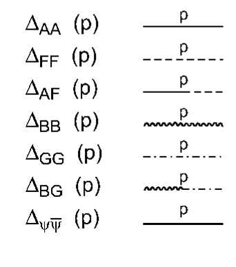
FIG. 3.: Graphical representation for the propagators.

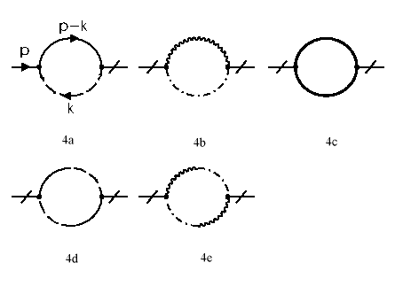
FIG. 4.: One–loop contributions to the self-energy of the $A$ field.

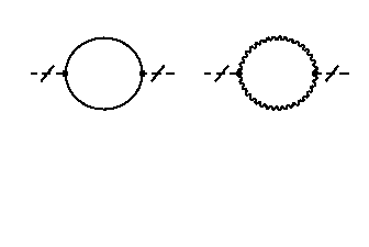
FIG. 5.: One–loop corrections to the two point function of the auxiliary field $F$.

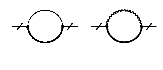
FIG. 6.: One–loop contributions to the self-energy of the spinor field $\psi$.

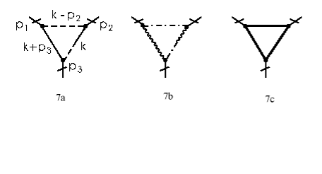
FIG. 7.: Divergent graphs contributing to the three point function of the $A$ field.

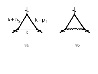
FIG. 8.: One–loop contributions to the three point function $\Gamma(A\overline{\psi}\psi)$

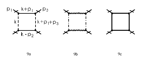
FIG. 9.: Divergent graphs contributing to the four point function of the $A$ field.

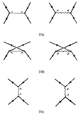
FIG. 10.: Lowest order graphs contributing to the scattering of two Majorana spinors.

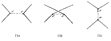
FIG. 11.: Lowest order graphs contributing to the scattering of two $A$-quanta.