Casimir effect in Domain Wall formation

Abstract

The Casimir forces on two parallel plates in conformally flat de Sitter background due to conformally coupled massless scalar field satisfying mixed boundary conditions on the plates is investigated. In the general case of mixed boundary conditions formulae are derived for the vacuum expectation values of the energy-momentum tensor and vacuum forces acting on boundaries. Different cosmological constants are assumed for the space between and outside of the plates to have general results applicable to the case of domain wall formations in the early universe.

1 Introduction

The Casimir effect is one of the most interesting manifestations of nontrivial properties of the vacuum state in quantum field theory [1,2]. Since its first prediction by Casimir in 1948[2] this effect has been investigated for different fields having different boundary geometries[3-5]. The Casimir effect can be viewed as the polarization of vacuum by boundary conditions or geometry. Therefore, vacuum polarization induced by a gravitational field is also considered as Casimir effect.
In the context of hot big bang cosmology, the unified theories of the fundamental interactions predict that the universe passes through a sequence of phase transitions. These phase transitions can give rise to domain structures determined by the topology of the manifold $M$ of degenerate vacuua [6, 7, 8]. If $M$ is disconnected, i.e. if $\pi(M)$ is nontrivial, then one can pass from one ordered phase to the other only by going through a domain wall. If $M$ has two connected components, e.g. if there is only a discrete reflection symmetry with $\pi_{0}(M)=Z_{2}$, then there will be just two ordered phase separated by a domain wall. In the domain wall formation models, in the early universe, the space-time changes from de Sitter to the geometry induced by the presence of a domain wall. In [9] the effects of particle production and vacuum polarization attendant to the domain wall formation have been studied. Casimir stress for parallel plates in the background of static domain wall in four and two dimensions is calculated in [10, 11]. Spherical bubbles immersed in different de Sitter spaces in- and out-side is calculated in [12, 13].
Our aim is to calculate the Casimir stress on two parallel plates with constant comoving distance having different vacuums between and outside, i.e. with false/true vacuum between/outside. Our model may be used to study the effect of the Casimir force on the dynamics of the domain wall formation appearing in the simplest Goldston model. In this model potential of the scalar field has two equal minima corresponding to degenerate vacuua. Therefore, scalar field maps points at spatial infinity in physical space nontrivially into the vacuum manifold [14]. Domain walls occur at the boundary between these regions of space. One may assume that the outer regions of parallel plates are in $\Lambda_{out}$ vacuum corresponding to degenerate vacuua in domain wall configuration. Previously this method has been used in [15] to drive the vacuum stress on parallel plates for scalar field with Dirichlet boundary condition in de Sitter space. For Neumann or more general mixed boundary conditions we need to have the Casimir energy-momentum tensor for the flat spacetime counterpart in the case of the Robin boundary conditions with coefficients related to the metric components of the brane-world geometry and the boundary mass terms. The Casimir effect for the general Robin boundary conditions on background of the Minkowski spacetime was investigated in Ref. [16] for flat boundaries. Here we use the results of Ref. [16] to generate vacuum energy–momentum tensor for the plane symmetric conformally flat backgrounds. Also this method has been used in [17] to derive the vacuum characteristics of the Casimir configuration on background of conformally flat brane-world geometries for massless scalar field with Robin boundary condition on plates.
In section two we calculate the stress on two parallel plates with Robin boundary conditions. The case of different de Sitter vacuua between and outside of the plates, is considered in section three. The last section conclude and summarize the results.

2 Vacuum expectation values for the energy-momentum tensor

We will consider a conformally coupled massless scalar field $\varphi(x)$ satisfying the equation

$$\left(\nabla_{\mu}\nabla^{\mu}+\frac{1}{6}R\right)\varphi(x)=0,$$ (1)

on background of a de Sitter space-time. In Eq. (1) $\nabla_{\mu}$ is the operator of the covariant derivative, and $R$ is the Ricci scalar for the de Sitter space.

$$R=\frac{12}{\alpha^{2}},$$ (2)

To make the maximum use of the flat space calculation we use the de Sitter metric in the conformally flat form:

$$ds^{2}=\frac{\alpha^{2}}{\eta^{2}}[d\eta^{2}-\sum_{\imath=1}^{3}(dx^{\imath})^{2}],$$ (3)

where $\eta$ is the conformal time:

$$\infty<\eta<0.$$ (4)

The relation between parameter $\alpha$ and cosmological constant $\Lambda$ is given by

$$\alpha^{2}=\frac{3}{\Lambda}.$$ (5)

We will assume that the field satisfies the mixed boundary condition

$$\left(a_{j}+b_{j}n^{\mu}\nabla_{\mu}\right)\varphi(x)=0,\quad z=z_{j},\quad j=1,2$$ (6)

on the plate $z=z_{1}$ and $z=z_{2}$, $z_{1}<z_{2}$, $n^{\mu}$ is the normal to these surfaces, $n_{\mu}n^{\mu}=-1$, and $a_{j}$, $b_{j}$ are constants. The results in the following will depend on the ratio of these coefficients only. However, to keep the transition to the Dirichlet and Neumann cases transparent we will use the form (6). For the case of plane boundaries under consideration introducing a new coordinate $y$ in accordance with

$$dy=\frac{\alpha}{\eta}dz$$ (7)

conditions (6) take the form

$$\left(a_{j}+(-1)^{j-1}b_{j}\frac{\eta}{\alpha}\partial_{z}\right)\varphi(x)=\left(a_{j}+(-1)^{j-1}b_{j}\partial_{y}\right)\varphi(x)=0,\quad y=y_{j},\quad j=1,2.$$ (8)

Note that the Dirichlet and Neumann boundary conditions are obtained from Eq. (6) as special cases corresponding to $(a_{j},b_{j})=(1,0)$ and $(a_{j},b_{j})=(0,1)$ respectively. The Robin boundary condition may be interpreted as the boundary condition on a thick plate [18]. Rewriting Eq.(8) in the following form

$$\varphi(x)=-(-1)^{j-1}\frac{b_{j}}{a_{j}}\partial y\varphi(x),$$ (9)

where $\frac{a_{j}}{b_{j}}$, having the dimension of a length, may be called skin-depth parameter. This is similar to the case of penetration of an electromagnetic field into a real metal, where the tangential component of the electric field is proportional to the skin-depth parameter.
Our main interest in the present paper is to investigate the vacuum expectation values (VEV’s) of the energy–momentum tensor for the field $\varphi(x)$ in the region $z_{1}<z<z_{2}$. The presence of boundaries modifies the spectrum of the zero–point fluctuations compared to the case without boundaries. This results in the shift in the VEV’s of the physical quantities, such as vacuum energy density and stresses. This is the well known Casimir effect. It can be shown that for a conformally coupled scalar by using field equation (1) the expression for the energy–momentum tensor can be presented in the form

$$T_{\mu\nu}=\nabla_{\mu}\varphi\nabla_{\nu}\varphi-\frac{1}{6}\left[\frac{g_{\mu\nu}}{2}\nabla_{\rho}\nabla^{\rho}+\nabla_{\mu}\nabla_{\nu}+R_{\mu\nu}\right]\varphi^{2},$$ (10)

where $R_{\mu\nu}$ is the Ricci tensor. The quantization of a scalar filed on background of metric Eq.(3) is standard. Let $\{\varphi_{\alpha}(x),\varphi_{\alpha}^{\ast}(x)\}$ be a complete set of orthonormalized positive and negative frequency solutions to the field equation (1), obying boundary condition (6). By expanding the field operator over these eigenfunctions, using the standard commutation rules and the definition of the vacuum state for the vacuum expectation values of the energy-momentum tensor one obtains

$$\langle 0|T_{\mu\nu}(x)|0\rangle=\sum_{\alpha}T_{\mu\nu}\{\varphi{{}_{\alpha},\varphi_{\alpha}^{\ast}\}},$$ (11)

where $|0\rangle$ is the amplitude for the corresponding vacuum state, and the bilinear form $T_{\mu\nu}\{{\varphi,\psi\}}$ on the right is determined by the classical energy-momentum tensor (10). In the problem under consideration we have a conformally trivial situation: conformally invariant field on background of the conformally flat spacetime. Instead of evaluating Eq. (11) directly on background of the curved metric, the vacuum expectation values can be obtained from the corresponding flat spacetime results for a scalar field $\bar{\varphi}$ by using the conformal properties of the problem under consideration. Under the conformal transformation $g_{\mu\nu}=\Omega^{2}\eta_{\mu\nu}$ the $\bar{\varphi}$ field will change by the rule

$$\varphi(x)=\Omega^{-1}\bar{\varphi}(x),$$ (12)

where for metric Eq.(3) the conformal factor is given by $\Omega=\frac{\alpha}{\eta}$. The boundary conditions for the field $\bar{\varphi}(x)$ we will write in form similar to Eq. (8)

$$\left(\bar{a}_{j}+(-1)^{j-1}\bar{b}_{j}\partial_{z}\right)\bar{\varphi}=0,\quad z=z_{j},\quad j=1,2,$$ (13)

with constant Robin coefficients $\bar{a}_{j}$ and $\bar{b}_{j}$. Comparing to the boundary conditions (6) and taking into account transformation rule (12) we obtain the following relations between the corresponding Robin coefficients

$$\bar{a}_{j}=a_{j}-(-1)^{j-1}\frac{b_{j}}{\alpha},\quad\bar{b}_{j}=b_{j}\frac{\eta}{\alpha}$$ (14)

Note that as Dirichlet boundary conditions are conformally invariant the Dirichlet scalar in the curved bulk corresponds to the Dirichlet scalar in a flat spacetime. However, for the case of Neumann scalar the flat spacetime counterpart is a Robin scalar with $\bar{a}_{j}=(-1)^{j-1}\frac{1}{\eta}$ and $\bar{b}_{j}=1$. The Casimir effect with boundary conditions (13) on two parallel plates on background of the Minkowski spacetime is investigated in Ref. [16] for a scalar field with a general conformal coupling parameter. In the case of a conformally coupled scalar the corresponding regularized VEV’s for the energy-momentum tensor are uniform in the region between the plates and have the form

$$\langle\bar{T}_{\nu}^{\mu}\left[\eta_{\alpha\beta}\right]\rangle_{{\rm ren}}=-\frac{J_{3}(B_{1},B_{2})}{8\pi^{3/2}a^{4}\Gamma(5/2)}{\rm diag}(1,1,1,-3),\quad z_{1}<z<z_{2},$$ (15)

where

$$J_{3}(B_{1},B_{2})={\rm p.v.}\int_{0}^{\infty}\frac{t^{3}dt}{\frac{(B_{1}t-1)(B_{2}t-1)}{(B_{1}t+1)(B_{2}t+1)}e^{2t}-1},$$ (16)

and we use the notations

$$B_{j}=\frac{\bar{b}_{j}}{\bar{a}_{j}a},\quad j=1,2,\quad a=z_{2}-z_{1}.$$ (17)

For the Dirichlet scalar $B_{1}=B_{2}=0$ and one has $J_{D}(0,0)=2^{-4}\Gamma(4)\zeta_{R}(4)$, with the Riemann zeta function $\zeta_{R}(s)$. Note that in the regions $z<z_{1}$ and $z>z_{2}$ the Casimir densities vanish [10, 16]:

$$\langle\bar{T}_{\nu}^{\mu}\left[\eta_{\alpha\beta}\right]\rangle_{{\rm ren}}=0,\quad z<z_{1},z>z_{2}.$$ (18)

This can be also obtained directly from Eq. (15) taking the limits $z_{1}\rightarrow-\infty$ or $z_{2}\rightarrow+\infty$. The values of the coefficients $B_{1}$ and $B_{2}$ for which the denominator in the subintegrand of Eq. (15) has zeros are specified in [16]. The vacuum energy-momentum tensor on de Sitter space Eq.(3) is obtained by the standard transformation law between conformally related problems (see, for instance, [19]) and has the form

$$\langle T_{\nu}^{\mu}\left[g_{\alpha\beta}\right]\rangle_{{\rm ren}}=\langle T_{\nu}^{\mu}\left[g_{\alpha\beta}\right]\rangle_{{\rm ren}}^{(0)}+\langle T_{\nu}^{\mu}\left[g_{\alpha\beta}\right]\rangle_{{\rm ren}}^{(b)}.$$ (19)

Here the first term on the right is the vacuum energy–momentum tensor for the situation without boundaries (gravitational part), and the second one is due to the presence of boundaries. As the quantum field is conformally coupled and the background spacetime is conformally flat the gravitational part of the energy–momentum tensor is completely determined by the trace anomaly and is related to the divergent part of the corresponding effective action by the relation [19]

$$\langle T_{\nu}^{\mu}\left[g_{\alpha\beta}\right]\rangle_{{\rm ren}}^{(0)}=2g^{\mu\sigma}(x)\frac{\delta}{\delta g^{\nu\sigma}(x)}W_{{\rm div}}[g_{\alpha\beta}].$$ (20)

The boundary part in Eq. (19) is related to the corresponding flat spacetime counterpart (15),(18) by the relation [19]

$$\langle T_{\nu}^{\mu}\left[g_{\alpha\beta}\right]\rangle_{{\rm ren}}^{(b)}=\frac{1}{\sqrt{|g|}}\langle\bar{T}_{\nu}^{\mu}\left[\eta_{\alpha\beta}\right]\rangle_{{\rm ren}}.$$ (21)

By taking into account Eq. (15) from here we obtain

$$\langle T_{\nu}^{\mu}\left[g_{\alpha\beta}\right]\rangle_{{\rm ren}}^{(b)}=-\frac{\eta^{4}J_{3}(B_{1},B_{2})}{8\pi^{3/2}a^{4}\Gamma(5/2)\alpha^{4}}{\rm diag}(1,1,1,-3),$$ (22)

for $z_{1}<z<z_{2}$, and

$$\langle T_{\nu}^{\mu}\left[g_{\alpha\beta}\right]\rangle_{{\rm ren}}^{(b)}=0,\;{\rm for}\;z<z_{1},z>z_{2}.$$ (23)

In Eq. (22) the constants $B_{j}$ are related to the Robin coefficients in boundary condition (6) by formulae (17),(14) and are functions on $z_{j}$. In particular, for Neumann boundary conditions $B^{(N)}_{j}=(-1)^{j-1}\eta/a$.

The first term in Eq.(18) is the vacuum polarization due to the gravitational field, without any boundary conditions, which can be rewritten as following

$$\langle T_{\nu}^{\mu}\left[g_{\alpha\beta}\right]\rangle_{{\rm ren}}^{(0)}=-\frac{1}{2880}[\frac{1}{6}\tilde{H}^{(1)\mu}_{\nu}-\tilde{H}^{(3)\mu}_{\nu}]$$ (24)

The functions $H^{(1,3)\mu}_{\nu}$ are some combinations of curvature tensor components (see [19]). For massless scalar field in de Sitter space, the term is given by [19, 20]

$$-\frac{1}{2880}[\frac{1}{6}\tilde{H}^{(1)\mu}_{\nu}-\tilde{H}^{(3)\mu}_{\nu}]=\frac{1}{960\pi^{2}\alpha^{4}}\delta^{\mu}_{\nu}.$$ (25)

The gravitational part of the pressure according to Eq.(25) is equal to

$$P_{g}=-<T^{1}_{1}>=\frac{-1}{960\pi^{2}\alpha^{4}}.$$ (26)

This is the same from both sides of the plates, and hence leads to zero effective force. Therefore the effective force acting on the plates are given only by the boundary part of the vacuum pressure , $p_{b}=-\langle T_{3}^{3}\left[g_{\alpha\beta}\right]\rangle_{{\rm ren}}^{(b)}$, taken at the point $z=z_{j}$:

$$p_{bj}(z_{1},z_{2})=-\frac{\eta^{4}J_{3}(B_{1},B_{2})}{4\alpha^{4}\pi^{3/2}a^{4}\Gamma(3/2)}=-\frac{\eta^{4}\Lambda^{2}J_{3}(B_{1},B_{2})}{36\pi^{3/2}a^{4}\Gamma(3/2)}.$$ (27)

This corresponds to the attractive/repulsive force between the plates if $p_{bj}</>0$. The equilibrium points for the plates correspond to the zero values of Eq. (27): $p_{bj}=0$. These points are zeros of the function $J_{3}(B_{1},B_{2})$ defined by Eq. (16) and are the same for both plates.

3 Parallel plates with different cosmological constants between and out-side

Now, assume there are different vacuua between and out-side of the plates, corresponding to $\alpha_{betw}$ and $\alpha_{out}$ in the metric Eq.(3). As we have seen in the last section, the vacuum pressure due to the boundary is only non-vanishing between the plates. Therefore, we have for the pressure due to the boundary

$$p_{bj}(z_{1},z_{2})=-\frac{\eta^{4}J_{3}(B_{1},B_{2})}{4\alpha_{betw}^{4}\pi^{3/2}a^{4}\Gamma(3/2)}=-\frac{\eta^{4}\Lambda_{betw}^{2}J_{3}(B_{1},B_{2})}{36\pi^{3/2}a^{4}\Gamma(3/2)}.$$ (28)

Now, the effective pressure created by gravitational part Eq.(25), is different for different part of the space-time:

$$P^{betw}_{g}=-<T^{1}_{1}>_{betw}=\frac{-1}{960\pi^{2}\alpha_{betw}^{4}}=\frac{-\Lambda_{betw}^{2}}{9}\frac{1}{960\pi^{2}},$$ (29)

$$P^{out}_{g}=-<T^{1}_{1}>_{out}=\frac{-1}{960\pi^{2}\alpha_{out}^{4}}=\frac{-\Lambda_{out}^{2}}{9}\frac{1}{960\pi^{2}}.$$ (30)

Therefore, the gravitational pressure acting on the plates is given by

$$P_{g}=P^{betw}_{g}-P^{out}_{g}=\frac{-1}{9\times 960\pi^{2}}(\Lambda_{betw}^{2}-\Lambda_{out}^{2}).$$ (31)

The total pressure acting on the plates, $P$, is then given by

$$P=P_{g}+P_{b}=\frac{-1}{9\times 960\pi^{2}}(\Lambda_{betw}^{2}-\Lambda_{out}^{2})-\frac{\eta^{4}\Lambda_{betw}^{2}J_{3}(B_{1},B_{2})}{36\pi^{3/2}a^{4}\Gamma(3/2)}.$$ (32)

In figures $1,2$, I have plotted the vacuum boundary pressure (second summand in Eq.(32)) acting per unit surface of the plates as functions of $a_{p}/\tilde{B_{2}}$ where $a_{p}=a\alpha_{betw}/\eta$ is the proper distance between the plates, which is given by

$$a_{p}=\int_{z_{1}}^{z_{2}}\sqrt{-g_{33}}dz=a\alpha_{betw}/\eta$$ (33)

and, $\tilde{B_{i}}=B_{i}/a_{p}$ (note that $\tilde{B_{i}}$ do not depend on $\eta$ and $a$). Fig1 for $\tilde{B_{1}}=0$ and fig2 for $\tilde{B_{1}}=\tilde{B_{2}}$. The first case is also presented in paper by Saharian and Romeo [16].

As a result we have an example for the stabilization of the distance between the plates due to the vacuum boundary pressures. But in this case total pressure may be negative or positive. To see the different possible cases, let us first assume a false vacuum between the plates, and true vacuum out-side, i.e. $\Lambda_{betw}>\Lambda_{out}$, then the gravitational part is negative, $p_{g}<0$, depending to the boundary part pressure the following cases can be occur

$$P_{b}>0,\hskip 14.22636ptP_{b}>|p_{g}|\Rightarrow p>0,$$ (34)

$$P_{b}>0,\hskip 14.22636ptP_{b}=|p_{g}|\Rightarrow p=0,$$ (35)

$$P_{b}>0,\hskip 14.22636ptP_{b}<|p_{g}|\Rightarrow p<0,$$ (36)

$$P_{b}=0\Rightarrow p<0,\hskip 28.45274ptP_{b}<0\Rightarrow p<0.$$ (37)

For the case of true vacuum between the plates and false vacuum out-side, i.e. $\Lambda_{betw}<\Lambda_{out}$, the gravitational pressure is positive $p_{g}>0$. In this case the following possibility can be occur

$$P_{b}<0,\hskip 14.22636pt|P_{b}|<p_{g}\Rightarrow p>0,$$ (38)

$$P_{b}<0,\hskip 14.22636pt|P_{b}|>p_{g}\Rightarrow p<0,$$ (39)

$$P_{b}<0,\hskip 14.22636pt|P_{b}|=p_{g}\Rightarrow p=0,$$ (40)

$$P_{b}>0,\Rightarrow p>0,\hskip 28.45274ptP_{b}=0\Rightarrow p>0.$$ (41)

As one can see in Eqs.(35, 40) the boundary part and gravitational part pressure cancel each other out, in this case the plates are fixed and we have stable equilibrium points. In the cases with $p</>0$, the initial attraction /repulsion of the parallel plates may be stopped or not depending on the detail of the dynamics.

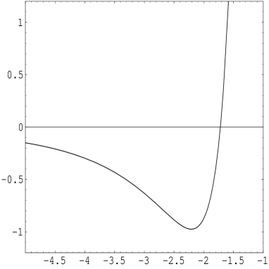
Figure 1: Boundary part of pressure as a function on $a_{p}/\tilde{B_{2}}$ , when $\tilde{B_{1}}=0$.

Figure 2: Boundary part of pressure as a function on $a_{p}/\tilde{B_{2}}$ , when $\tilde{B_{1}}=\tilde{B_{2}}$.

4 Conclusion

In the present paper we have investigated the Casimir effect for a conformally coupled massless scalar field confined in the region between two parallel plate with constant comoving distance on background of the conformally-flat de Sitter spacetimes. The general case of the mixed(Robin) boundary conditions is considered. The vacuum expectation values of the energy-momentum tensor are derived from the corresponding flat spacetime results by using the conformal properties of the problem. In the region between the plates the boundary induced part for the vacuum energy-momentum tensor is given by Eq.(22), and the corresponding vacuum forces acting per unit surface of the plates have the form Eq. (27). These forces vanish at the zeros of the function $J_{3}(B_{1},B_{2})$.The vacuum polarization due to the gravitational field, without any boundary conditions is given by Eq.(25), the corresponding gravitational pressure part has the form Eq.(26), which is the same from both sides of the plates, and hence leads to zero effective force. Further we consider different cosmological constants for the space between and outside of the plates, in this case the effective pressure created by gravitational part is different for different part of the space-time and add to the boundary part pressure. Our calculation shows that the detail dynamics of the plates depends on different parameters and all cases of attraction and repulsion may appear. The result may be of interest in the case of formation of the cosmic domain walls in early universe, where the wall orthogonal to the $z-$axis is described by the function $\Phi_{i}(z)$ interpolating between two different minima at $z\rightarrow\pm\infty$ [14].

References

- [1] G. Plunien, B. Mueller, W. Greiner, Phys. Rep. 134, 87(1986).
- [2] H. B. G. Casimir, proc. K. Ned. Akad. Wet. 51, 793(1948).
- [3] E. Elizalde, S. D. Odintsov, A. Romeo, A. A. Bytsenko and S. Zerbini, zeta regularization techniques with applications(World Scientific, Singapore, 1994).
- [4] E. Elizalde, Ten physical applications of spectral zeta functions, lecture notes in physics, (Springer-Verlage, Berlin, 1995).
- [5] V. M. Mostepanenko and N. N. Trunov. The Casimir effect and its applications. (Oxford Science Publications New York, 1997).
- [6] Ya. B. Zel’dovich, I. Yu. Kobzarev and L. B. Okun, Sov. Phys. JETP 40, 1 (1975).
- [7] T. W. B. Kibble, J. Phys. A9, 1387 (1976).
- [8] A. Vilenkin, Phys. Reports 121, 263 (1985).
- [9] P. R. Anderson, W. A. Hiscock and R. Holman, Phys. Rev. D41, 3604(1990).
- [10] M. R. Setare and A. A. Saharian. Int. J. Mod. Phys. A16, 1463(2001).
- [11] M. R. Setare and A. H. Rezaeian. Mod. Phys. Lett. A15, 2159(2000).
- [12] M. R. Setare and R. Mansouri. Class. Quant. Grav. 18 (2001) 2331.
- [13] M. R. Setare .Class. Quant. Grav. 18 (2001) 4823-4830.
- [14] A. Vilenkin and E. P. S. Shellard. COSMIC STRINGS AND OTHER TOPOLOGICAL DEFFECTS,(Cambridge University Press, 1994).
- [15] M. R. Setare and R. Mansouri. Class. Quant. Grav. 18 (2001),2659.
- [16] A. Romeo and A. A. Saharian, J. Phys. bf A35 (2002) 1297-1320.
- [17] A. A. Saharian, M. R. Setare, Phys. Lett. B552, 119, (2003).
- [18] S. L. Lebedev, Vacuum energy and Casimir force in a presence of skin-depth dependent bondary condition,hep-th/0003229.
- [19] N. D. Birrell and P. C. W. Davies, Quantum fields in curved space,( Chambridge University press, 1986).
- [20] J. S. Dowker, R. Critchley, Phys. Rev. D13, 3224 (1976).