Cosmological perturbations and the transition from contraction to expansion

Abstract

We investigate both analytically and numerically the evolution of scalar perturbations generated in models which exhibit a smooth transition from a contracting to an expanding Friedmann universe. If the perturbation equations are formulated as second order equations for either the Bardeen potential $\Psi$ or the curvature perturbation on uniform comoving hypersurfaces $\zeta$, at best one of them can stay regular during the transition. We find that the resulting spectral index in the late radiation dominated universe depends on which of these two variables passes regularly through the transition. The results can be parametrized by the exponent $q$ defining the rate of contraction of the universe, or equivalently through the equation of state $w=(2-q)/3q$ of the background fluid. For $q\geqslant-\frac{1}{2}$ we find that there are no stable cases where both $\Psi$ and $\zeta$ are regular during the transition. In particular, for $0<q\ll 1$, we find that the resulting spectral index is close to scale invariant if $\Psi$ is regular, whereas it has a steep blue behavior if $\zeta$ is regular. We also show that as long as $q\leqslant 1$, perturbations remain small during contraction in the sense that there exists a gauge in which all the metric and matter perturbation variables are small. This work has important implications for the current debate concerning the nature of perturbations evolving through a collapsing regime into an expanding one: it shows that if in the ekpyrotic model, where $0<q\ll 1$, the Bardeen potential passes regularly through the transition, this leads to a nearly scale invariant spectrum with $n=1-2q$, whereas in the case of dilaton-driven string cosmology we have the opposite situation. There it is assumed that $\zeta$ passes regularly through the transition, leading to a very blue spectrum of highly suppressed perturbations.

I Introduction

Recently, it has been argued that a slowly contracting universe which transits smoothly over to an expanding radiation dominated era may lead to a scale invariant spectrum of adiabatic density fluctuations Khoury:2001zk ; Durrer:2002jn ; Peter:2002cn ; Khoury:2001wf . There has been quite an intense debate on the question of whether the resulting spectrum after the transition to the radiation era indeed is scale invariant or whether it has a steep blue spectrum with $n\simeq 3$. The latter result has been advocated mainly by Brandenberger:2001bs ; Lyth:2001pf ; Hwang:2001ga . Gratton et al. have now gone further arguing that the ekpyrotic or cyclic scenario is the only robust case where a scale-invariant spectra can be found (along with inflation for the case of an expanding universe) Gratton:2003pe .

If the equations of motion governing the transition for the background and the perturbations were known, this problem could be solved by integrating them numerically. However it is likely that the evolution in this high curvature regime will contain full string theory and we do not even know whether the variables of the low energy theory are appropriate for the description of this regime. One possibility which has been studied in the past is the inclusion of first order corrections in the string scale $\alpha^{\prime}$ and/or the coupling constant $g_{s}$ (see, e.g. Antoniadis:1994jc ; Brustein:1998cv ; Foffa:1999dv ; Cartier:1999vk ). In this context it has been shown that, within a certain range of coefficients for the terms added to the tree level Lagrangian, one can exit from the high curvature regime and enter into a radiation dominated phase Cartier:1999vk . In Cartier:2001is the corrections of the perturbation equations have been derived and have been solved for dilaton-driven string cosmology. Lately, Tsujikawa et al. Tsujikawa:2002qc have used these equations to study the ekpyrotic model Khoury:2001wf ; Khoury:2001zk . Even though they have followed the perturbations through a regularized transition, we will argue that their method invariably leads to $n\simeq 3$ and does not allow for a decision whether a blue, $n\simeq 3$ or a scale-invariant, $n\simeq 1$ spectrum of perturbations is obtained. In this paper we first study a general transition which satisfies relatively mild criteria and we formulate conditions for the transition which lead to either of the two spectral indices. We can decide under which conditions either the spectral index $n=1$ as advocated by Durrer and Vernizzi Durrer:2002jn or $n=3$ put forward in Finelli:2001sr and others is obtained in the ekpyrotic model. This model is a special case of the more general class of contracting universes discussed here.

The rest of this paper is organized as follows: In Sec. II we present the aspects of cosmological perturbation theory needed in this paper. We then discuss the transition from a contracting to an expanding phase emphasizing the differences between such a transition and that associated with the transition between a conventional inflationary phase to radiation. We also formulate the problem encountered when inferring the perturbation spectrum after the transition from the one before the transition. In Sec. III we study the behavior of perturbations during a transition and find that the resulting spectral index depends on mutually excluding, simple regularity conditions for the transition, which we formulate in detail.

In Sec. IV we study numerical toy models for the transition where we exemplify the general results obtained in the previous section and analyze the stability of the numerically obtained spectral indices. Then we formulate our regularity condition as a theorem and we study the amplitude of perturbations. In Sec. V we comment on the findings in previous work and we summarize our results.

II Background and perturbations in simple contracting and expanding universes

In this section we repeat the basic equations for the Friedmann background and adiabatic first order perturbations. We then discuss initial conditions for perturbations in a contracting universe and explain how a different spectral index is obtained depending on the perturbation variable used for the transition.

II.1 The background

We consider a Friedmann universe with negligible spatial curvature, which is first contracting for $-\infty<\eta<-\eta_{s}$ and hence its (spacetime) curvature is growing. The variable $\eta$ denotes conformal time and $\eta_{s}>0$ is the moment when we enter a high-curvature regime. We call this period the “pre-big-bang phase”. At $\eta\sim-\eta_{s}$ corrections coming from some underlying theory, which reduces to general relativity when the curvature is sufficiently small, become important and we assume that they regularize the geometry and lead to an expanding universe at $\eta>\eta_{s}$. We also assume that radiation is produced during the transition so that for $\eta>\eta_{s}$ (the “post-big-bang” phase) the universe can be described as a radiation dominated Friedmann universe. In the pre- and post-big-bang phases, $|\eta|\gg\eta_{s}$, we have

$${\cal H}^{2} = \frac{\kappa^{2}}{3}\rho a^{2}~{},$$ (1)

$${\cal H}^{\prime} = -{\kappa^{2}\over 6}(\rho+3P)a^{2}=-{\cal H}^{2}\frac{1+3w}{2}~{},$$ (2)

where the equation of state of the background fluid is $w=P/\rho$ and $\kappa^{2}=8\pi G=2/M_{P}^{2}$. $M_{P}=1/\sqrt{4\pi G}=3.4\times 10^{18}$ GeV is the reduced Planck mass. ${\cal H}=a^{\prime}/a=\dot{a}=Ha$ is the comoving Hubble parameter. A prime denotes a derivative with respect to conformal time $\eta$, whereas a dot denotes a derivative with respect to physical time $t$, defined by $dt=ad\eta$. We shall also use

$$w^{\prime}=3(w-c_{s}^{2})(1+w){\cal H}\quad\mbox{ where }\quad c_{s}^{2}=\left(\frac{dP}{d\rho}\right)_{\scriptsize{\textrm{ad}}}$$ (3)

is the adiabatic sound speed (if $\rho\neq$ const, $c_{s}^{2}=P^{\prime}/\rho^{\prime}$). We will be especially interested in phases during which $P/\rho=w=$ const. Then $c_{s}^{2}=$ const $=w$ and the scale factor evolves like a power law,

$$a=\left|\frac{\eta}{\eta_{s}}\right|^{q}~{},\qquad q=\frac{2}{1+3w}~{}.$$ (4)

An inflationary phase, defined by $1+3w<0$, is thus realized when $q<0$. During the radiation dominated post-big-bang phase $w=1/3$, hence $q=1$.

We will consider a scalar field dominated pre-big-bang phase. During this phase we have

$$\rho={\varphi^{\prime 2}\over 2a^{2}}+V(\varphi)~{},\qquad P={\varphi^{\prime 2}\over 2a^{2}}-V(\varphi)~{},$$ (5)

so that

$$w+1={{\varphi^{\prime}}^{2}\over 3{\cal H}^{2}}~{}.$$ (6)

For a scalar field, $w$ is constant only for the following possibilities:

$$w=\left\{\begin{array}[]{lll}1&\mbox{ if }&V=0~{},\\ -1&\mbox{ if }&\varphi^{\prime}=0~{},\\ \lambda^{2}/3-1&\mbox{ if }&V=V_{0}\exp(-\lambda\varphi)~{},\quad V_{0}\neq 0~{},\end{array}\right.$$ (7)

and, correspondingly,

$$q=\left\{\begin{array}[]{lll}1/2&\mbox{ if }&V=0~{},\\ -1&\mbox{ if }&\varphi^{\prime}=0~{},\\ \frac{2}{\lambda^{2}-2}&\mbox{ if }&V=V_{0}\exp(-\lambda\varphi)~{},\quad V_{0}\neq 0~{}.\end{array}\right.$$ (8)

II.2 Perturbations

We now discuss perturbation theory in a Friedmann universe (neglecting spatial curvature, $K=0$) with a scalar field or a perfect fluid, like radiation.

We first consider the linear perturbation equation for the Bardeen potential (see, e.g. Mukhanov:1992tc ; Durrer:1993db ):

$$\Psi^{\prime\prime}+3{\cal H}(1+c_{s}^{2})\Psi^{\prime}+\left[2{\cal H}^{\prime}+(1+3c_{s}^{2}){\cal H}^{2}-\Upsilon\Delta\right]\Psi=0~{}.$$ (9)

This equation is valid for adiabatic perturbations of a fluid, with $\Upsilon=c_{s}^{2}$, or for a simple scalar field, with $\Upsilon=1$ (see, e.g. Mukhanov:1992tc ).

If we define the canonical variable

$$u={M_{P}a\over\sqrt{{\cal H}^{2}-{\cal H}^{\prime}}}\Psi~{},$$ (10)

$u$ satisfies the equation Mukhanov:1992tc

$$u^{\prime\prime}+(\Upsilon k^{2}-\theta^{\prime\prime}/\theta)u=0~{},$$ (11)

for

$$\begin{array}[]{lcl}&&\theta=\theta_{1}={{\cal H}\over a\sqrt{{2\over 3}({\cal H}^{2}-{\cal H}^{\prime})}}~{},\\ \mbox{or}&&\\ &&\theta=\theta_{2}=\theta_{1}\int{d\eta\over\theta_{1}^{2}}~{}.\end{array}$$ (12)

If we restrict ourselves to the case $w=c_{s}^{2}=$ const, the mass term in Eq. (9), namely, $2{\cal H}^{\prime}+(1+3c_{s}^{2}){\cal H}^{2}$, vanishes by the use of the background Einstein equations (1) and (2). For these backgrounds which have $a\propto|\eta|^{q}$, where $q$ is given in Eq. (4), we find

$$\Psi^{\prime\prime}+2{\cal H}{1+q\over q}\Psi^{\prime}+\Upsilon k^{2}\Psi=0~{}.$$ (13)

The $u$ equation then simply becomes a Bessel differential equation,

$$u^{\prime\prime}+\left(\Upsilon k^{2}-{q(q+1)\over\eta^{2}}\right)u=0~{}.$$ (14)

The correct normalization to the incoming vacuum at $\eta\to-\infty$ determines the initial conditions such that (see, e.g. Durrer:2002jn )

$$u={\sqrt{\pi|k\eta|}\over k^{3/2}}H_{\mu}^{(2)}(k\eta)~{},$$ (15)

with $\mu=q+1/2$. Here $H_{\mu}^{(2)}$ denotes the Hankel function of the second kind and of order $\mu$. At “late times” when $|k\eta|\ll 1$ but still $\eta\ll-\eta_{s}$ we may neglect the $k^{2}$ term in Eq. (14) and find the super-Hubble scale solution

$$u=A_{-}\left|\frac{\eta}{\eta_{s}}\right|^{-q}+B_{-}\left|\frac{\eta}{\eta_{s}}\right|^{1+q}=u_{A}+u_{B}~{}.$$ (16)

The coefficients $A_{-}$ and $B_{-}$ are determined by the initial solution (15),

$$A_{-}\simeq k^{-3/2}(k\eta_{s})^{-q}~{},\quad B_{-}\simeq k^{-3/2}(k\eta_{s})^{1+q}~{},$$ (17)

hence they have the spectra Durrer:2002jn

$$P_{A_{-}} = |A_{-}|^{2}k^{3}\simeq(k\eta_{s})^{-2q}\propto k^{n_{A_{-}}-1}~{},\quad~{}n_{A_{-}}=1-2q~{},$$ (18)

$$P_{B_{-}} = |B_{-}|^{2}k^{3}\simeq(k\eta_{s})^{2+2q}\propto k^{n_{B_{-}}-1}~{},\quad n_{B_{-}}=3+2q~{}.$$ (19)

Furthermore, $|u_{B}/u_{A}|\simeq|k\eta|^{1+2q}$. Hence for $q>-1/2$, the $A$ mode, $u_{A}$, dominates at late time over the $B$ mode, $u_{B}$.

Another perturbation variable often used is the curvature perturbation on uniform comoving hypersurfaces Lyth:1985aa

$$\zeta={{\cal H}\Psi^{\prime}+{\cal H}^{2}\Psi\over{\cal H}^{2}-{\cal H}^{\prime}}+\Psi~{}.$$ (20)

A simple substitution using Eq. (9) and the background equations yields

$$\zeta^{\prime}=-k^{2}{\Upsilon{\cal H}\over{\cal H}^{2}-{\cal H}^{\prime}}\Psi~{},$$ (21)

hence on super-Hubble scales, $|k/{\cal H}|\ll 1$, this variable is conserved. For ordinary inflationary models, it is therefore usually sufficient to compute $\zeta$ at the time of the Hubble radius crossing during inflation to obtain its value in the radiation dominated era. Furthermore, since during radiation $\zeta=(3/2)\Psi$, this simply gives the Bardeen potential.

The evolution of $\zeta$ is closely related to the canonical variable $v$ defined by

$$v=-{M_{P}a\sqrt{{\cal H}^{2}-{\cal H}^{\prime}}\over\sqrt{\Upsilon}{\cal H}}\zeta~{}.$$ (22)

This variable satisfies the equation Mukhanov:1992tc

$$v^{\prime\prime}+(\Upsilon k^{2}-z^{\prime\prime}/z)v=0~{},$$ (23)

where

$$\begin{array}[]{lcl}&&z=z_{1}={a\sqrt{{\cal H}^{2}-{\cal H}^{\prime}}\over\sqrt{\Upsilon}{\cal H}}~{},\\ \mbox{or}&&\\ &&z_{2}=z_{1}\int{d\eta\over z_{1}^{2}}~{}.\end{array}$$ (24)

Note that the relation between $v$ and $\zeta$ is $v=-M_{P}z_{1}\zeta$. Equation (23) is invariant under the “duality” $z_{1}\to z_{2}$, in the same way as Eq. (11) is invariant under $\theta_{1}\to\theta_{2}$.

In Mukhanov:1992tc it is shown that $v$ appears in the perturbed action as a canonical scalar variable. Hence on sub-Hubble scales, $|k/{\cal H}|\gg 1$, it satisfies the initial condition $v_{in}=\exp(-ik\eta)/\sqrt{k}$.

As before, we now concentrate on the case $w=c_{s}^{2}=$ const, with the scale factor given in Eq. (4). Then

$$z_{1}\propto a\quad\mbox{ and }\quad v={\rm const}\times M_{P}a\zeta~{},$$ (25)

and the constant of order unity depends on $q$ and $\Upsilon$.

During the pre-big-bang phase Eq. (23) then also becomes a Bessel differential equation,

$$v^{\prime\prime}+\left(k^{2}-{q(q-1)\over\eta^{2}}\right)v=0~{}.$$ (26)

We have set $\Upsilon=1$ throughout the evolution, which should be fine as we are considering mainly super-Hubble terms, which satisfy $k^{2}\Upsilon\ll z^{\prime\prime}/z$ during the transition. We have confirmed in numerical simulations that allowing $\Upsilon$ to vary during the evolution does not affect the key results we present which concern the spectral index.

The solution with the correct initial conditions is

$$v={\sqrt{\pi|k\eta|}\over k^{1/2}}H_{\nu}^{(2)}(k\eta)~{},$$ (27)

with $\nu=1/2-q$. At “late times” when $|k\eta|\ll 1$ but still $\eta\ll-\eta_{s}$ we may neglect the $k^{2}$ term in Eq. (26) and find the super-Hubble scale solution

$$v=C_{-}\left|\frac{\eta}{\eta_{s}}\right|^{1-q}+D_{-}\left|\frac{\eta}{\eta_{s}}\right|^{q}=v_{C}+v_{D}~{}.$$ (28)

The coefficients $C_{-}$ and $D_{-}$ are determined by the initial solution (27),

$$C_{-}\simeq(k\eta_{s})^{\nu}\eta_{s}^{1/2}~{},\quad D_{-}\simeq(k\eta_{s})^{-\nu}\eta_{s}^{1/2}~{}.$$ (29)

The spectra obtained depend on the value of $q$. One finds Durrer:2002jn

$$P_{C_{-}} = |C_{-}|^{2}k^{3}\simeq(k\eta_{s})^{4-2q}\eta_{s}^{-2}\propto k^{n_{C_{-}}-1}~{},\quad\,n_{C_{-}}=5-2q~{},$$ (30)

$$P_{D_{-}} = |D_{-}|^{2}k^{3}\simeq(k\eta_{s})^{2+2q}\eta_{s}^{-2}\propto k^{n_{D_{-}}-1}~{},\quad n_{D_{-}}=3+2q~{}.$$ (31)

Here $|v_{C}/v_{D}|\simeq|k\eta|^{1-2q}$, hence the $D$ mode dominates for $q<1/2$, while the $C$ mode dominates for $q>1/2$. Finally we want to note that $u$ and $v$ are related via

$$v = {-\theta_{1}\over\sqrt{\Upsilon}}(u/\theta_{1})^{\prime}~{},$$ (32)

$$u = {z_{1}\over k^{2}\sqrt{\Upsilon}}(v/z_{1})^{\prime}~{}.$$ (33)

It is interesting to note that from the lowest order approximations for $u$ and $v$ given in Eqs. (16), (28) the equivalences (32) and (33) of $u$ and $v$ cannot be recovered. Only when we go to the next order in the term proportional to $\theta_{1}$ or $z_{1}$, respectively (or when using the full Bessel function solution) does the above equivalence give $u_{A}\longleftrightarrow v_{C}$ and $u_{B}\longleftrightarrow v_{D}$ along with

$$n_{A}+4=n_{C}~{},\qquad n_{B}=n_{D}~{}.$$ (34)

II.3 The problem of a transition from contraction to expansion

Let us first consider the case where $q$ is in the interval $-1/2\leqslant q\leqslant 1/2$. Even though $q<0$ does not represent a contracting phase, no difference of the following arguments arises from letting $q$ decrease until $-1/2$ (usual inflation has $q\,\raise 1.72218pt\hbox{$>$}\kern-6.99997pt\lower 2.6694pt\hbox{$\sim$}\,-1$).

Comparing the amplitudes of the modes of $u$ and $v$, we see that at the transition to the expansion phase, $|\eta|\sim\eta_{s}$, we have $u_{A}\gg u_{B}$ and $v_{D}\gg v_{C}$ for cosmologically interesting scales with $k\sim 1/\eta_{0}\sim 10^{-30}/\eta_{P}$. Here $\eta_{0}$ denotes the value of conformal time today and $\eta_{P}=M_{P}^{-1}$. Naively, we therefore expect that immediately after the transition

$$u\simeq A_{-}\quad\mbox{and}\quad v\simeq D_{-}\quad\mbox{ for }\quad-1/2\leqslant q\leqslant 1/2~{}.$$ (35)

Since in the radiation dominated era $u\propto\eta^{2}$ and $v\propto\eta$ on super-Hubble scales, we expect during the radiation phase

$$u\simeq A_{-}(\eta/\eta_{s})^{2}\quad\mbox{ and }\quad v\simeq D_{-}(\eta/\eta_{s})\quad\mbox{ for }\quad k\eta\ll 1~{}.$$ (36)

From the relations of $u$ and $\Psi$ as well as $v$ and $\zeta$ during the radiation dominated phase, this gives

$$\Psi\simeq\sqrt{2}~{}A_{-}/(\eta_{s}M_{P})\quad\mbox{ and }\quad\zeta\simeq D_{-}/M_{P}~{}.$$ (37)

For $q\neq-1/2$, this naive result is clearly in contradiction with the fact that during the radiation dominated era $\Psi$ and $\zeta$ differ only by a constant since, according to Eqs. (18) and (31), $\Psi$ would have the spectral index $n_{\Psi}=n_{A_{-}}=1-2q$ while $\zeta$ would have the spectral index $n_{\zeta}=n_{D_{-}}=3+2q$.

For $q\leqslant-1/2$ the $B$ mode of $u$, $u_{B}$ dominates (for $q=-1/2$, $u_{A}$ and $u_{B}$ are of the same order) and we expect $\Psi$ to have the spectrum $n_{\Psi}=n_{B_{-}}=3+2q=n_{D_{-}}=n_{\zeta}$, hence we obtain the same spectrum as $\zeta$ in the radiation era, so that there is no contradiction.

For $q>1/2$ the $C$ mode of $v$, $v_{C}$ dominates and hence $\zeta$ actually has the spectrum $n_{\zeta}=n_{C_{-}}=5-2q$, which is in even worse disagreement with the naively expected spectrum for $\Psi$. This contradictory situation is shown on the right hand panel of Fig. 1. Since for ordinary inflation $q\sim-1$, this problem has never been realized when studying usual inflation.

The simplest possibility which could resolve the issue is to note that the decaying mode of $u$ ($q>-1/2$) during the pre-big-bang phase, $u_{B}$, has the same spectrum as $v_{D}$. Hence if the $u$-growing mode during the pre-big-bang phase is entirely converted into the decaying mode after the transition and therefore cannot be seen late in the post-big-bang era, we expect the spectrum $n=3+2q$ in the radiation era. This argument has been put forward in Brandenberger:2001bs , where the authors have shown that this is exactly what happens if the transition is defined by a vanishing jump in the metric and the second fundamental form on the constant energy hypersurface. Similar arguments have also been presented in Lyth:2001pf ; Hwang:2001ga . They led these authors to the conclusion that the correct spectrum, evaluated sufficiently long after the pre $\to$ post transition so that the decaying mode has died away, is $n=n_{\Psi}=n_{\zeta}=3+2q$. If this is correct the spectrum of the ekpyrotic model is very blue and in contradiction to the observed close-to-scale invariant spectrum. The same argument for the original pre-big-bang model of Veneziano Veneziano:1991ek ; Gasperini:2002bn , where the scalar field potential vanishes and hence $q=1/2$, led to the conclusion that the dilaton perturbation spectrum is very blue with $n=4$ Brustein:1995kn ; Deruelle:1995kd .

In Durrer:2002jn this argument has been criticized for two main reasons. First, the background second fundamental form given by ${\cal H}/a$ has to jump, even to change sign, in a transition from contraction to expansion. It then seems quite unnatural to require its perturbation to vanish. Second, if the matching conditions are posed on an only slightly different hypersurface, the naively expected spectral index, $n_{\Psi}=1-2q$ is obtained. This ’‘instability” of the index $n_{\Psi}=3+2q$ will also be illustrated in Sec. IV with numerical studies of a simple toy model.

The above argument cannot be used if $q>1/2$ because $u$ has no mode with spectral index $5-2q$. In this case, agreement can only be achieved if the dominant contribution to $v$, $v_{D}$, is also transferred entirely into the decaying mode so that late after the transition $v$ and hence $\zeta$ still have the spectral index $n_{D_{-}}=3+2q$. However, this is not possible: As one easily concludes, e.g. from Brandenberger:2001bs or Lyth:2001pf , a transition on the constant energy hypersurface, where the growing mode of $u$ is transferred completely into the decaying mode, preserves $\zeta$, hence $\zeta$ has the same spectrum after the transition as before, $n_{\zeta}=5-2q$ which does not agree with the spectrum of $\Psi$ which in this case is $n_{\Psi}=3+2q$.

Hence if the transition is such that both $\Psi$ and $\zeta$ correspond after the transition to one of their modes before the transition, the obtained spectral index must be $n=3+2q$. As we have shown, this cannot happen for $q>1/2$ if the transition is “simple”, i.e. does not modify the spectrum of either $\Psi$ or $\zeta$.

If the spectral index after the transition is $n=1-2q$ as promoted in Durrer:2002jn for $q>-1/2$, the variable $\zeta$ makes a $k$-dependent jump at the transition. If $n=5-2q$ is obtained as in Finelli:2001sr , $\Psi$ makes a $k$-dependent jump. Furthermore, if $n=3+2q$ is obtained for $q>-1/2$, the growing mode of $\Psi$ before the transition has to be converted entirely into the decaying mode. For $q>1/2$ also this no longer helps resolve the problem, and one of the two variables $\zeta$ or $\Psi$ must be modified in a $k$-dependent way during the transition.

III General solutions of the perturbation equations through the transition

Having explained the problem, but before discussing possible resolutions, let us collect some generic facts about a transition from contraction to expansion. Clearly, to have such a transition ${\cal H}$, ${\cal H}^{\prime}$ and $\dot{H}=({\cal H}/a)^{\prime}/a=({\cal H}^{\prime}-{\cal H}^{2})/a^{2}$ have to change sign. Within the framework of general relativity (neglecting spatial curvature) this requires $\rho+P<0$ and therefore cannot be achieved with a scalar field (with standard kinetic term). If a positive spatial curvature is added, the scalar field initial condition can be fine tuned such that close to the collapse the curvature term dominates over the scalar field contributions, and a transition from contraction to expansion can be achieved with a standard scalar field Page:1984 .

In this section we want to discuss the problem outlined above without specifying any details of the transition. For this, we first discuss the linear second order differential equation

$$x^{\prime\prime}+\left(k^{2}-V_{x}\right)x=0~{},\qquad V_{x}={s^{\prime\prime}\over s}~{},$$ (38)

which we have encountered in the previous section. Here the variables $(x,s)$ stand for either $(u,\theta)$ or $(v,z)$. The factor $\Upsilon$ in front of the $k^{2}$ term is disregarded since it is irrelevant for our considerations which mainly concern super-Hubble scales. We notice that Eq. (38) is invariant under the duality transformation $s=s_{1}\to s_{1}\int d\eta/s_{1}^{2}\equiv s_{2}$. If $s$ is a power law, $s_{1}=\left|\eta/\eta_{s}\right|^{\gamma}$, we can set $s_{2}=\left|\eta/\eta_{s}\right|^{1-\gamma}$. The duality property of Eq. (38) has been discussed in Wands:1998yp . If $s$ and $1/s$ are bounded in the interval $[\eta_{in},\eta]$, so that

$$\infty>C=\max_{\{\eta_{in}\leqslant\eta_{1}\leqslant\eta\}}\Big{(}s(\eta_{1})^{2},1/s(\eta_{1})^{2}\Big{)}~{},$$ (39)

this equation has the general solution Brustein:1998kq ; Gasperini:2002bn

$$x=s\Big{[}\alpha{\rm Tcos}(s,k)+\beta{\rm Tsin}(s,k)\Big{]}~{},$$ (40)

where ${\rm Tcos}$ and ${\rm Tsin}$ are defined by

$${\rm Tcos}(s,k) \equiv 1-k^{2}\int_{\eta_{in}}^{\eta}{d\eta_{1}\over s^{2}(\eta_{1})}\int_{\eta_{in}}^{\eta_{1}}d\eta_{2}s^{2}(\eta_{2})$$ (41)

$$+k^{4}\int_{\eta_{in}}^{\eta}{d\eta_{1}\over s^{2}(\eta_{1})}\int_{\eta_{in}}^{\eta_{1}}d\eta_{2}s^{2}(\eta_{2})\int_{\eta_{in}}^{\eta_{2}}{d\eta_{3}\over s^{2}(\eta_{3})}\int_{\eta_{in}}^{\eta_{3}}d\eta_{4}s^{2}(\eta_{4})-k^{6}\cdots\quad,$$

$${\rm Tsin}(s,k) \equiv k\int_{\eta_{in}}^{\eta}{d\eta_{1}\over s^{2}(\eta_{1})}$$ (42)

$$-k^{3}\int_{\eta_{in}}^{\eta}{d\eta_{1}\over s^{2}(\eta_{1})}\int_{\eta_{in}}^{\eta_{1}}d\eta_{2}s^{2}(\eta_{2})\int_{\eta_{in}}^{\eta_{2}}{d\eta_{3}\over s^{2}(\eta_{3})}+k^{5}\cdots\quad.$$

When expressing a given solution in terms of ${\rm Tcos}$ and ${\rm Tsin}$ the coefficients $\alpha$ and $\beta$ will depend on the initial value $\eta_{in}$ chosen. But as long as $s$ and $1/s$ are bounded, the sums (41) and (42) always converge since the terms in this sum are bounded, e.g. by the terms in the series expansion for $\cos\left[Ck(\eta-\eta_{in})\right]$ and $\sin\left[Ck(\eta-\eta_{in})\right]$, respectively. Here $C$ is the bound from Eq. (39) above.

To relate this solution with the results of Sec. II.3, we choose $\eta_{in}$ such that $k|\eta_{in}|\ll 1$, but $\eta_{in}\ll-\eta_{s}$. If $s$ obeys a simple power law, $s=|\eta/\eta_{s}|^{\gamma}$, hence $s^{\prime\prime}/s=\gamma(\gamma-1)/\eta^{2}$, we obtain to lowest order

$${\rm Tcos}(s,k)=1~{},$$ (43)

and

$${\rm Tsin}(s,k)={k\eta_{s}\over 1-2\gamma}\left[\left|\frac{\eta_{in}}{\eta_{s}}\right|^{1-2\gamma}-\left|\frac{\eta}{\eta_{s}}\right|^{1-2\gamma}\right]~{},$$ (44)

so that

$$x=\left[\alpha+{\beta k\eta_{s}\over 1-2\gamma}\left|\frac{\eta_{in}}{\eta_{s}}\right|^{1-2\gamma}\right]\left|\frac{\eta}{\eta_{s}}\right|^{\gamma}-\beta{k\eta_{s}\over 1-2\gamma}\left|\frac{\eta}{\eta_{s}}\right|^{1-\gamma}~{}.$$ (45)

(For $\gamma=1/2$ the powers in the ${\rm Tsin}$ integral becomes a logarithm, but we shall neglect this logarithmic correction here.) There are several facts to note at this point:

• Only two of the three parameters $\eta_{in},\alpha,\beta$ which determine the initial conditions are independent.

• As in Eqs. (12), (24), two pump fields $s_{1}$ and $s_{2}$ yield the same potential $V_{x}$ in Eq. (38). If $\eta_{in}$ is chosen such that the contributions to the integrals from the lower boundary can be neglected, changing $s$ from $s_{1}$ to $s_{2}$ transforms ${\rm Tcos}$ into $k^{-1}{\rm Tsin}$ and ${\rm Tsin}$ into $k{\rm Tcos}$.

• If $s\propto\eta^{\gamma}$ is a pure power law and again the contributions from the lower boundary can be neglected, ${\rm Tcos}\propto\sqrt{k|\eta|}J_{\nu}(|k\eta|)$ and ${\rm Tsin}\propto\sqrt{k|\eta|}Y_{-\nu}(|k\eta|)$, where $\nu=\gamma-1/2$ and $J,~{}Y$ are Bessel functions.

We now define

$$y\equiv\frac{s}{k^{2}}\left(x/s\right)^{\prime}~{}.$$ (46)

Using Eq. (38), we find

$$\pmatrix{y\cr y^{\prime}}=-\frac{1}{k^{2}}\pmatrix{\frac{s^{\prime}}{s}&-1\cr k^{2}-\left(\frac{s^{\prime}}{s}\right)^{2}&\frac{s^{\prime}}{s}}\pmatrix{x\cr x^{\prime}}~{},$$ (47)

which we can invert to obtain

$$\pmatrix{x\cr x^{\prime}}=-\pmatrix{\frac{s^{\prime}}{s}&1\cr-k^{2}+\left(\frac{s^{\prime}}{s}\right)^{2}&\frac{s^{\prime}}{s}}\pmatrix{y\cr y^{\prime}}~{}.$$ (48)

Using the latter and Eq. (38), the evolution equation for the variable $y$ can be derived

$$y^{\prime\prime}+\left[\frac{s^{\prime\prime}}{s}-2\left(\frac{s^{\prime}}{s}\right)^{2}\right]y+k^{2}y=0~{}.$$ (49)

Let us now introduce

$$r\equiv s^{-1}\left[c_{1}+c_{2}\int^{\eta}{s}^{2}d\tilde{\eta}\right]~{},$$ (50)

so that

$$r^{\prime}=-\frac{{s}^{\prime}}{s}r+c_{2}{s}~{},\qquad r^{\prime\prime}=-\left[\frac{{s}^{\prime\prime}}{{s}}-2\left(\frac{{s}^{\prime}}{s}\right)^{2}\right]r~{}.$$ (51)

Equation (49) then takes the simple form

$$y^{\prime\prime}+\left(k^{2}-{V}_{y}\right)y=0~{},\qquad{V}_{y}\equiv\frac{r^{\prime\prime}}{r}~{}.$$ (52)

Note that the $y$ equation obtained from a given $x$ equation depends on our choice of $s$. Since $s_{1}^{\prime\prime}/s_{1}=s_{2}^{\prime\prime}/s_{2}$ but $s_{1}^{\prime}/s_{1}\neq s_{2}^{\prime}/s_{2}$, $V_{y}=-s^{\prime\prime}/s+2(s^{\prime}/s)^{2}$ depends on this choice. Such a “dual variable” $y$ can also be found if $k^{2}$ is modified into $\Upsilon(\eta)k^{2}$, the expressions just become somewhat more complicated. Choosing $x=v$ and $s=z_{1}$, Eqs. (47), (48) just reproduce the relations (32), (33) where $y=u$ and $r=\theta$. During a power law evolution of the scale factor, we have $z_{1}=\left|\eta/\eta_{s}\right|^{q}$, $z_{2}=\left|\eta/\eta_{s}\right|^{1-q}$, $\theta_{1}=\left|\eta/\eta_{s}\right|^{-q}$ and $\theta_{2}=\left|\eta/\eta_{s}\right|^{1+q}.$

As we have seen in the previous section, on large scales, $|k\eta|\ll 1$, the general solution of Eq. (38) is to lowest order of the form

$$x={\cal A}\left|\frac{\eta}{\eta_{s}}\right|^{\gamma}+{\cal B}\left|\frac{\eta}{\eta_{s}}\right|^{1-\gamma}+{\cal O}(|k\eta|^{2})~{},$$ (53)

where one obtains from Eq. (45)

$$\alpha = {\cal A}+{\cal B}\left|\frac{\eta_{in}}{\eta_{s}}\right|^{1-2\gamma}~{},$$ (54)

$$\beta = -{{\cal B}(1-2\gamma)\over k\eta_{s}}~{}.$$ (55)

To discuss what might happen during a transition we now assume that for a given $s=s_{1}$ or $s_{2}$ the solution (40) can be continued through the transition to the radiation era, the only effect of the transition being a modification of $s$ which interpolates from

$$s=|\eta/\eta_{s}|^{\gamma_{-}}\quad\mbox{ for }\quad\eta\ll-\eta_{s}~{},$$ (56)

to

$$s=|\eta/\eta_{s}|^{\gamma_{+}}\quad\mbox{ for }\quad\eta\gg\eta_{s}~{},$$ (57)

without passing through zero. At some time $\eta_{s}\ll\eta\ll 1/k$ in the radiation era, we still can approximate the ${\rm Tcos}$ and ${\rm Tsin}$ integrals by the first term in their series expansion (41,42). Integrating the first term in Eq. (42), we obtain

$$x = \left[\alpha+{\beta k\eta_{s}\over 1-2\gamma_{-}}\left(\Delta_{T}-{2-2\gamma_{-}-2\gamma_{+}\over 1-2\gamma_{+}}+\left|\frac{\eta_{in}}{\eta_{s}}\right|^{1-2\gamma_{-}}\right)\right]\left({\eta\over\eta_{s}}\right)^{\gamma_{+}}$$ (58)

$$+{\beta k\eta_{s}\over 1-2\gamma_{+}}\left({\eta\over\eta_{s}}\right)^{1-\gamma_{+}}~{}.$$

Here

$$\Delta_{T}={1-2\gamma_{-}\over\eta_{s}}\int_{-\eta_{s}}^{\eta_{s}}s^{-2}d\tilde{\eta}$$ (59)

comes from the contribution to the integral during the transition. We always assume that the free normalization of $s$ is chosen such that $s(-\eta_{s})=1$. The dimensionless, $k$-independent constant $\Delta_{T}$ is then the only quantity that incorporates our ignorance of the true form of the transition. Although its typical order of magnitude is ${\cal O}(\Delta_{T})={\cal O}(1)$, we will mention explicit limits on $\Delta_{T}$ as we go along. With the above expressions for $\alpha$ and $\beta$ we have

$$x=\left[{\cal A}-{\cal B}\left(\Delta_{T}-{2-2\gamma_{-}-2\gamma_{+}\over 1-2\gamma_{+}}\right)\right]\left({\eta\over\eta_{s}}\right)^{\gamma_{+}}-{\cal B}{1-2\gamma_{-}\over 1-2\gamma_{+}}\left({\eta\over\eta_{s}}\right)^{1-\gamma_{+}}~{},$$ (60)

which is independent of $\eta_{in}$ as it should be.

In what follows we will study eight different cases and compute the resulting spectra. For the first four cases we shall assume that $u$ remains regular throughout. Recalling the notation that $\theta_{-}$ refers to the collapsing phase and $\theta_{+}$ to the expanding phase in Eqs. (11), (12), we shall consider the following possibilities: $\theta_{1-}=|\eta/\eta_{s}|^{-q}$ goes over smoothly into $\theta_{1+}=(\eta/\eta_{s})^{-1}$ (case 1); $\theta_{1-}$ goes over smoothly into $\theta_{2+}=(\eta/\eta_{s})^{2}$ (case 2); $\theta_{2-}=|\eta/\eta_{s}|^{1+q}$ goes over smoothly into $\theta_{1+}$ (case 3) and $\theta_{2-}$ goes over smoothly into $\theta_{2+}$ (case 4). We shall then study the equivalent cases for $v$ with $\theta$ replaced by $z$ in Eqs. (23), (24). We are mainly interested in a contracting pre-big-bang phase, $q>0$, but the results derived here are valid also for $-1/2<q$.

Case 1:   $\gamma_{-}=-q$, $\gamma_{+}=-1$.
Here we have ${\cal A}=A_{-}$ and ${\cal B}=B_{-}$, hence

$$u \simeq k^{-3/2}\left\{\left[(k\eta_{s})^{-q}-(k\eta_{s})^{1+q}\left(\Delta_{T}-{2(2+q)\over 3}\right)\right]\left({\eta\over\eta_{s}}\right)^{-1}\right.$$ (61)

$$\quad\quad\quad\left.~{}-{1+2q\over 3}(k\eta_{s})^{1+q}\left({\eta\over\eta_{s}}\right)^{2}\right\}~{}.$$

If $\Delta_{T}$ is of order unity, or more precisely if

$$\Delta_{T}~{}\,\raise 1.72218pt\hbox{$<$}\kern-8.00003pt\lower 2.6694pt\hbox{$\sim$}\,~{}(k\eta_{s})^{-(1+2q)}~{},$$ (62)

the resulting spectrum as well as the amplitude does not depend on $\Delta_{T}$ and we have

$$|u|^{2}k^{3}\simeq\left\{\begin{array}[]{lcl}(k\eta_{s})^{-2q}\left({\eta\over\eta_{s}}\right)^{-2}&\mbox{ for }k<k_{u}(\eta){}&n=1-2q~{},\\ \left({1+2q\over 3}\right)^{2}(k\eta_{s})^{2+2q}\left({\eta\over\eta_{s}}\right)^{4}&\mbox{ for }k>k_{u}(\eta){}&n=3+2q~{},\end{array}\right.$$ (63)

where

$$k_{u}(\eta)\simeq\eta^{-1}\left({\eta\over\eta_{s}}\right)^{(2q-2)/(2q+1)}$$ (64)

is the wave number where we see a kink in the spectrum. For a value of $q$ in the regime of our primary interest, $-1/2<q<1$, the exponent $(2q-2)/(2q+1)$ is negative and $k_{u}(\eta)\ll\eta^{-1}$ especially at late times, $\eta\gg\eta_{s}$. Hence, in this case the spectral index relevant for the observed anisotropies in the cosmic microwave background (CMB) is $n=3+2q$, a steep blue spectrum. In reaching this conclusion, we have used the fact that in the radiation era,

$$\Psi \simeq {\sqrt{2}\eta_{s}\over M_{P}\eta^{2}}u~{},$$ (65)

$$|\Psi|^{2}k^{3} \simeq \left({M_{s}\over M_{P}}\right)^{2}(k\eta_{s})^{2+2q}~{}\mbox{ for }k>k_{u}(\eta)~{},\quad n=3+2q~{},$$ (66)

where we have introduced the transition mass scale, $M_{s}=\eta_{s}^{-1}$. For transitions from contraction to expansion, $q>0$, the amplitude of these fluctuations is therefore far too low to be of any relevance for cosmologically interesting scales, $k\simeq\eta_{0}^{-1}$. (Furthermore, the spectral index $n=3+2q$ is not consistent with observations.)

Case 2:   $\gamma_{-}=-q$, $\gamma_{+}=2$.
Since $\gamma_{-}$ is the same as in case 1, $\cal A$ and $\cal B$ remain unchanged. From Eq. (60), we find

$$u \simeq k^{-3/2}\left\{\left[(k\eta_{s})^{-q}-(k\eta_{s})^{1+q}\left(\Delta_{T}-{2(1-q)\over 3}\right)\right]\left({\eta\over\eta_{s}}\right)^{2}\right.$$ (67)

$$\quad\quad\quad\left.~{}+{1+2q\over 3}(k\eta_{s})^{1+q}\left({\eta\over\eta_{s}}\right)^{-1}\right\}~{},$$

so that

$$|u|^{2}k^{3} \simeq (k\eta_{s})^{-2q}\left({\eta\over\eta_{s}}\right)^{4},$$ (68)

$$|\Psi|^{2}k^{3} \simeq \left({M_{s}\over M_{P}}\right)^{2}(k\eta_{s})^{-2q}~{},\quad n=1-2q~{}.$$ (69)

For this result to apply, the condition on $\Delta_{T}$, Eq. (62) must be satisfied. If this case is realized and if $0<q\ll 1$, a scale invariant spectrum will be obtained. Its amplitude is determined by the transition scale which should be about 5 orders of magnitude below the Planck scale.

Case 3:   $\gamma_{-}=1+q$, $\gamma_{+}=-1$.
According to Eqs. (53) and (16), we now have ${\cal A}=B_{-}$ and ${\cal B}=A_{-}$. This leads to

$$u \simeq k^{-3/2}\left\{\left[(k\eta_{s})^{1+q}-(k\eta_{s})^{-q}\left(\Delta_{T}-{2(1-q)\over 3}\right)\right]\left({\eta\over\eta_{s}}\right)^{-1}\right.$$ (70)

$$\quad\quad\quad\left.~{}+{1+2q\over 3}(k\eta_{s})^{-q}\left({\eta\over\eta_{s}}\right)^{2}\right\}~{}.$$

We thus obtain

$$|u|^{2}k^{3} \simeq (k\eta_{s})^{-2q}\left({\eta\over\eta_{s}}\right)^{4}~{},$$ (71)

$$|\Psi|^{2}k^{3} \simeq \left({M_{s}\over M_{P}}\right)^{2}(k\eta_{s})^{-2q}~{},\quad n=1-2q~{},$$ (72)

as in case 2. Here this spectrum is obtained without any condition on $\Delta_{T}$ having to be satisfied, although for the correct amplitude to be obtained, we need $\Delta_{T}\,\raise 1.72218pt\hbox{$<$}\kern-8.00003pt\lower 2.6694pt\hbox{$\sim$}\,(\eta/\eta_{s})^{3}/3$.

Case 4:   $\gamma_{-}=1+q$, $\gamma_{+}=2$.
Again, we have we have ${\cal A}=B_{-}$ and ${\cal B}=A_{-}$ and so we obtain

$$u \simeq k^{-3/2}\left\{\left[(k\eta_{s})^{1+q}-(k\eta_{s})^{-q}\left(\Delta_{T}-{2(2+q)\over 3}\right)\right]\left({\eta\over\eta_{s}}\right)^{2}\right.$$ (73)

$$\quad\quad\quad\left.~{}-{1+2q\over 3}(k\eta_{s})^{-q}\left({\eta\over\eta_{s}}\right)^{-1}\right\}~{},$$

with

$$|u|^{2}k^{3} \simeq (k\eta_{s})^{-2q}\left(\Delta_{T}-{2(2+q)\over 3}\right)^{2}\left({\eta\over\eta_{s}}\right)^{4}~{},$$ (74)

$$|\Psi|^{2}k^{3} \simeq \left({M_{s}\over M_{P}}\right)^{2}(k\eta_{s})^{-2q}\left(\Delta_{T}-{2(2+q)\over 3}\right)^{2}~{},\quad n=1-2q~{}.$$ (75)

Again, we obtain a scale invariant spectrum if $q\ll 1$, but in this case the amplitude depends on the details of the transition given by $\Delta_{T}$.

We now repeat this analysis considering the alternative variable $v$ with ’pump field’ $s=z_{1}$ or $z_{2}$.

Case 1:   $\gamma_{-}=q$, $\gamma_{+}=1$.
According to Eqs. (53) to (55) we have ${\cal A}=D_{-}$ and ${\cal B}=C_{-}$, leading to

$$v = \sqrt{\eta_{s}}\left\{\left[(k\eta_{s})^{q-1/2}-(k\eta_{s})^{1/2-q}\left(\Delta_{T}-2q\right)\right]\left({\eta\over\eta_{s}}\right)+(1-2q)(k\eta_{s})^{1/2-q}\right\}~{},$$ (76)

$$|v|^{2}k^{3} \simeq \left\{\begin{array}[]{ll}\eta_{s}^{-2}(k\eta_{s})^{2+2q}\left({\eta\over\eta_{s}}\right)^{2}&\mbox{ for }q\leqslant 1/2~{},\\ \eta_{s}^{-2}(k\eta_{s})^{4-2q}\left(\Delta_{T}-2q\right)^{2}\left({\eta\over\eta_{s}}\right)^{2}&\mbox{ for }q>1/2~{},\end{array}\right.$$ (79)

$$|\zeta|^{2}k^{3} \simeq \left\{\begin{array}[]{ll}\left({M_{s}\over M_{P}}\right)^{2}(k\eta_{s})^{2+2q},&n=3+2q~{}\mbox{ if }~{}q\leqslant 1/2~{},\\ \left({M_{s}\over M_{P}}\right)^{2}(k\eta_{s})^{4-2q}\left(\Delta_{T}-2q\right)^{2},&n=5-2q~{}\mbox{ if }~{}q>1/2~{}.\end{array}\right.$$ (82)

If $q<1/2$ we must require $\Delta_{T}\,\raise 1.72218pt\hbox{$<$}\kern-8.00003pt\lower 2.6694pt\hbox{$\sim$}\,(k\eta_{s})^{2q-1}$ for our result to apply. Note also that the amplitude of the spectrum depends on the details of the transition given by $\Delta_{T}$ when $q>1/2$.

Case 2:   $\gamma_{-}=q$, $\gamma_{+}=0$.
Again, we have ${\cal A}=D_{-}$ and ${\cal B}=C_{-}$, which yields

$$v = \sqrt{\eta_{s}}\left\{\left[(k\eta_{s})^{q-1/2}-(k\eta_{s})^{1/2-q}\left(\Delta_{T}-2+2q\right)\right]-(1-2q)(k\eta_{s})^{1/2-q}\left({\eta\over\eta_{s}}\right)\right\}~{},$$ (83)

$$|v|^{2}k^{3} \simeq \left\{\begin{array}[]{ll}\eta_{s}^{-2}(k\eta_{s})^{4-2q}\left({\eta\over\eta_{s}}\right)^{2}&\mbox{ if }~{}q>1/2~{}\mbox{ or }~{}k>k_{v_{1}}(\eta)~{},\\ \eta_{s}^{-2}(k\eta_{s})^{2+2q}&\mbox{ if }~{}q\leqslant 1/2~{}\mbox{ and }~{}k<k_{v_{1}}(\eta)~{},\end{array}\right.$$ (86)

$$|\zeta|^{2}k^{3} \simeq \left\{\begin{array}[]{ll}\left({M_{s}\over M_{P}}\right)^{2}(k\eta_{s})^{4-2q}~{},&n=5-2q~{}\mbox{ if }~{}q>1/2~{}\mbox{ or }~{}k>k_{v_{1}}~{},\\ \left({M_{s}\over M_{P}}\right)^{2}(k\eta_{s})^{2+2q}\left({\eta\over\eta_{s}}\right)^{-2}~{},&n=3+2q~{}\mbox{ if }~{}q\leqslant 1/2~{}\mbox{ and }~{}k<k_{v_{1}}~{}.\end{array}\right.$$ (89)

For the result to apply when $q>1/2$ it requires $\Delta_{T}<\eta/\eta_{s}$. As in Case 1 of the $u$ field, there is a kink in the spectrum with the wave number of the kink for the case $q\leqslant 1/2$ being

$$k_{v_{1}}(\eta)=\eta^{-1}\left({\eta\over\eta_{s}}\right)^{-2q/(1-2q)}~{},$$ (90)

which is always smaller than the Hubble radius, $\eta^{-1}$, for the relevant values of $q$, $0<q<1/2$. Only for very small values of $q$, this kink in the spectrum lies very close to the Hubble radius and is not visible.

Case 3:   $\gamma_{-}=1-q$, $\gamma_{+}=1$.
Here we have ${\cal A}=C_{-}$ and ${\cal B}=D_{-}$, hence

$$v = \sqrt{\eta_{s}}\left\{\left((k\eta_{s})^{1/2-q}-(k\eta_{s})^{q-1/2}[\Delta_{T}-2+2q]\right)\left({\eta\over\eta_{s}}\right)-(k\eta_{s})^{q-1/2}(1-2q)\right\}~{},$$ (91)

$$|v|^{2}k^{3} \simeq \left\{\begin{array}[]{ll}\eta_{s}^{-2}(k\eta_{s})^{4-2q}\left({\eta\over\eta_{s}}\right)^{2}&\mbox{ if }~{}q>1/2~{},\\ \eta_{s}^{-2}(k\eta_{s})^{2+2q}\left({\eta\over\eta_{s}}\right)^{2}[\Delta_{T}-2+2q]^{2}&\mbox{ if }~{}q\leqslant 1/2~{},\end{array}\right.$$ (94)

$$|\zeta|^{2}k^{3} \simeq \left\{\begin{array}[]{ll}\left({M_{s}\over M_{P}}\right)^{2}(k\eta_{s})^{4-2q}~{},&n=5-2q~{}\mbox{ if }~{}q>1/2~{},\\ \left({M_{s}\over M_{P}}\right)^{2}(k\eta_{s})^{2+2q}[\Delta_{T}-2+2q]^{2}~{},&n=3+2q~{}\mbox{ if }~{}q\leqslant 1/2~{}.\end{array}\right.$$ (97)

For $q>1/2$ the amplitude of the resulting fluctuations does not depend on the details of the transition while it does depend on it for $q\leqslant 1/2$.

Case 4:   $\gamma_{-}=1-q$, $\gamma_{+}=0$.
Here again we have ${\cal A}=C_{-}$ and ${\cal B}=D_{-}$, so that

$$v = \sqrt{\eta_{s}}\left\{(k\eta_{s})^{1/2-q}-(k\eta_{s})^{q-1/2}[\Delta_{T}-2q]+(1-2q)(k\eta_{s})^{q-1/2}\left({\eta\over\eta_{s}}\right)\right\}~{},$$ (98)

$$|v|^{2}k^{3} \simeq \left\{\begin{array}[]{ll}\eta_{s}^{-2}(k\eta_{s})^{4-2q}&\mbox{ if }~{}q>1/2~{}\mbox{ and }~{}k<k_{v_{2}}~{},\\ \eta_{s}^{-2}(k\eta_{s})^{2+2q}\left({\eta\over\eta_{s}}\right)^{2}&\mbox{ if }~{}q\leqslant 1/2~{}\mbox{ or }~{}k<k_{v_{2}}~{},\end{array}\right.$$ (101)

$$|\zeta|^{2}k^{3} \simeq \left\{\begin{array}[]{ll}\left({M_{s}\over M_{P}}\right)^{2}(k\eta_{s})^{4-2q}\left({\eta\over\eta_{s}}\right)^{-2},&n=5-2q~{}\mbox{ if }~{}q>1/2\mbox{ and }k<k_{v_{2}}~{},\\ \left({M_{s}\over M_{P}}\right)^{2}(k\eta_{s})^{2+2q}~{},&n=3+2q~{}\mbox{ if }~{}q\leqslant 1/2\mbox{ or }k<k_{v_{2}}~{},\end{array}\right.$$ (104)

where here

$$k_{v_{2}}(\eta)\simeq\eta^{-1}\left({\eta\over\eta_{s}}\right)^{(2-2q)/(1-2q)}~{}.$$ (105)

For $1/2<q<1$ and $k_{v_{2}}<\eta^{-1}$, a kink from $n=3+2q$ to the final spectrum $n=5-2q$ is present in the spectral distribution.

In Tables 1–3 we summarize the results of our analysis:

The spectral index for a transition with regular $u$ and $q>-1/2$

case	$\gamma_{-}$	$\gamma_{+}$	kink?	stable?	ampl. depends	$n$
					on transition?
1	$-q$	$-1$	yes	no	no	$3+2q$
2	$-q$	$2$	no	yes	no	$1-2q$
3	$1+q$	$-1$	no	yes	no	$1-2q$
4	$1+q$	$2$	no	yes	yes	$1-2q$

Table 1: Here we summarize the post-big-bang spectral indices as a function of the pre- and post-big-bang exponent of the pump field, if $u$ is regular through the transition. The mild requirement on the transition ($\Delta_{T}$) for this to hold is mentioned in the text.

The spectral index for a transition with regular $v$ and $q\leqslant 1/2$

case	$\gamma_{-}$	$\gamma_{+}$	kink?	stable?	ampl. depends	$n$
					on transition?
1	$q$	$1$	no	yes	no	$3+2q$
2	$q$	$0$	yes	no	no	$5-2q$
3	$1-q$	$1$	no	yes	yes	$3+2q$
4	$1-q$	$0$	no	yes	no	$3+2q$

Table 2: Here we summarizes the post-big-bang spectral indices as a function of the pre- and post-big-bang exponent of the pump field, if $v$ is regular through the big bang and $q\leqslant 1/2$. The logarithmic corrections at $q=1/2$ are neglected. The mild requirement on the transition ($\Delta_{T}$) for this to hold is mentioned in the text.

The spectral index for a transition with regular $v$ and $q>1/2$

case	$\gamma_{-}$	$\gamma_{+}$	kink?	stable?	ampl. depends	$n$
					on transition?
1	$q$	$1$	no	yes	yes	$5-2q$
2	$q$	$0$	no	yes	no	$5-2q$
3	$1-q$	$1$	no	yes	no	$5-2q$
4	$1-q$	$0$	yes	no	no	$3+2q$

Table 3: Here we summarizes the post-big-bang spectral indices as a function of the pre- and post-big-bang exponent of the pump field, if $v$ is regular through the big bang and $q>1/2$. The mild requirement on the transition ($\Delta_{T}$) for this to hold is mentioned in the text.

From Eqs. (10) and (13) it is clear that during the radiation dominated era, inside the Hubble radius, $k\eta\gg 1$, the Bardeen potential oscillates and its amplitude decays like $1/\eta^{2}$, whereas during the matter dominated era, the Bardeen potential remains constant also inside the Hubble radius. Therefore, a change in the spectral index close to the Hubble radius crossing is not visible for scales which cross the Hubble radius in the radiation dominated era. This remark concerns mainly the kink in case 2 of Table 2.

A kink in the spectral distribution arises only in the unlikely situation where the growing mode of the pre-big-bang phase is fully converted into the decaying mode after the transition, and one has to wait a sufficiently long time $[\sim\eta(k)]$ for the decaying mode to decay and the final growing mode to dominate. It is only in such a situation that the final spectral index does not correspond to the naive expectation from the pre-big-bang phase. Finally, we note that a kink is always associated with an instability of the spectrum. The issue of stability will be discussed in Sec. IV where we model the regular behavior of $u$ and $v$ through simple toy models. There we shall see that a slight modification in the transition can change the spectral index $n=3+2q$ into $n=1-2q$ if $u$ passes through the transition regularly and $5-2q$ into $3+2q$ if $v$ is regular and $q\leqslant 1/2$, correspondingly $3+2q$ into $5-2q$ if $v$ is regular and $q>1/2$.

This brings us to one of the key results of this paper, a prediction of the spectral index arising from different conditions on $q$ and the regularity of the $u$ and $v$ fields:

$$n=\left\{\begin{array}[]{lcl}1-2q&\mbox{ if }&q>-1/2~{}\mbox{ and $u$ is regular and stable},\\ 3+2q&\mbox{ if }&q\leqslant 1/2~{}\mbox{ and $v$ is regular and stable},\\ 5-2q&\mbox{ if }&q>1/2~{}\mbox{ and $v$ is regular and stable},\\ 3+2q&\mbox{ if }&q\leqslant-1/2.\end{array}\right.$$ (106)

We have not treated explicitly the simple case $q<-1/2$ above, but this can be done exactly along the same lines as the other cases. From Eq. (106), we see that a scale-invariant spectrum is obtained for $q\simeq 1$ (standard inflation), or if $u$ is regular and $0<q\ll 1$, or if $v$ is regular and $q=2$. For this latter case, however, we shall see in Sec. V.2 that perturbations grow large during the contracting phase and therefore linear perturbation theory breaks down. Furthermore, such a collapsing universe with $q=2$ has been shown to be unstable Heard:2002dr .

Clearly, in a transition from contraction to expansion, it cannot be that both $u$ and $v$ are regular and stable if $q>-1/2$. Only in an inflationary transition with $q\leqslant-1/2$ do we find $n=3+2q$ for both $u$ and $v$. In this case it is expected that both variables transit in a regular stable fashion from inflation to the radiation era. The resulting spectral index does not depend on the variable with which the calculation is performed. The situation for arbitrary values of $q$ is shown in Fig. 1.

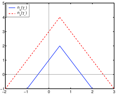
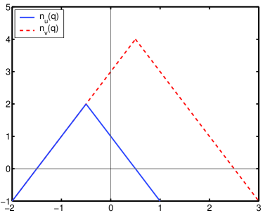
Figure 1: Here we illustrate the dominant spectral indices $n_{u}$ (solid) and $n_{v}$ (dashed) on super-Hubble scales which are obtained after a “stable”, regular transition of the corresponding variable to the radiation era at sufficiently late time. This is also the resulting spectral index for the Bardeen potential on cosmologically relevant scales. The left panel shows the indices as a function of $\gamma_{-}$, the exponent of the pump field during the pre-big-bang phase. The right panel shows them as a function of $q$, the exponent of the contraction (expansion) law before the big bang. We have used $\gamma_{u_{-}}=-q$ and $\gamma_{v_{-}}=q$.

IV Fast toy model transitions

In earlier work Cartier:1999vk ; Cartier:2001is ; Tsujikawa:2002qc a transition from contraction to expansion was achieved via a combination of first order corrections in the string scale $\alpha^{\prime}$ and/or the string coupling $g_{s}$. In Cartier:2001is a modified perturbation equation for $v$ was derived using this framework, and a spectral index $n=3+2q$ was obtained. This yields $n=4$ for the case dilaton-driven string cosmology Cartier:2001is where $q=1/2$, and $n=3$ for the ekpyrotic model Tsujikawa:2002qc where $q\sim 0$. However, although calculations have been performed with $v$, it remains to be shown that $u$ cannot pass through the transition regularly (to first order). Unfortunately, even though the perturbation equations of Cartier:2001is are very complicated, they are probably not realistic. It is clear that at a time where first order corrections become important, higher order corrections are likely to be relevant and the real behavior of the perturbations might differ significantly from the results obtained in the work cited above. In this sense, pre-big-bang models including first order corrections are only toy models.

In this section we confirm our generic findings concerning the spectral index associated with the relevant $u$ and $v$ fields by numerically solving a simple toy model. We do not insist on a physically well motivated transition. Rather we artificially define a regular scale factor so that it agrees with a contracting Friedmann universe with contraction exponent $q$ at $\eta\ll-\eta_{s}$ and with a radiation dominated universe at $\eta\gg\eta_{s}$. In the region in between, the scale factor smoothly evolves between contraction and expansion.

IV.1 The background

For the exact form of the regularized background scale factor we choose

$$a(\eta) = \left[\left(\eta/\eta_{s}\right)^{2}+\epsilon\right]^{\tilde{q}/2}~{},$$ (107)

$$\tilde{q}(\eta) = q\iota+(1-\iota)~{},$$ (108)

$$\iota(\eta) = 1/2-{1\over\pi}{\rm arctg}(\eta/\eta_{s})~{},$$ (109)

where $0<\epsilon\ll 1$. The function $\iota(\eta)$ could be replaced by any $C^{\infty}$ function which quickly interpolates between $1$ for $\eta\ll-\eta_{s}$ to $0$ for $\eta\gg\eta_{s}$. Clearly, this universe contracts like $|\eta|^{q}$ for $\eta\ll-\eta_{s}$ and expands like a radiation dominated universe $a\propto\eta$ for $\eta\gg\eta_{s}$. Furthermore, $a$, ${\cal H}$, ${\cal H}^{\prime}$ and ${\cal H}^{2}-{\cal H}^{\prime}$ are all regular, even analytic in the vicinity of the transition, $\eta=0$. The behavior of the relevant background quantities for our model are shown in Fig. 2.

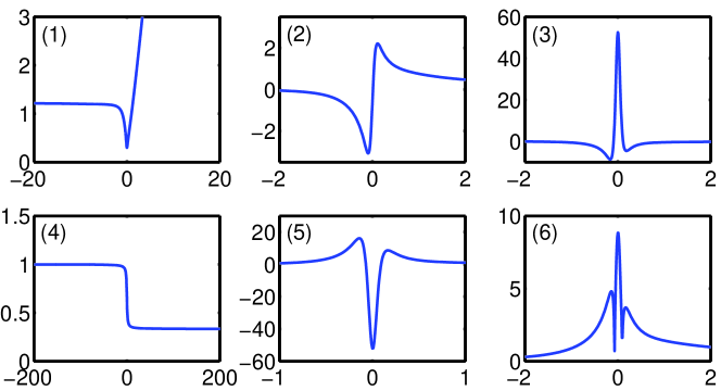
Figure 2: This figure illustrates the evolution of various background quantities scaled in such a way that they are dimensionless (i.e., invariant under a change in $\eta_{s}$). As functions of $\eta/\eta_{s}$, they are (1) the scale factor $a(\eta)$, (2) the Hubble rate ${\cal H}\eta_{s}$ and (3) its first time derivative ${\cal H}^{\prime}\eta_{s}^{2}$. On the bottom line, they are (4) the pre-factor of the comoving wave number $\Upsilon$, (5) the potential of the perturbation variable $u$, i.e., $V_{u}\eta_{s}^{2}=\left({\cal H}^{2}-{\cal H}^{\prime}\right)\eta_{s}^{2}$ and (6) its rescaled square root $\sqrt{|V_{u}|/\Upsilon}~{}\eta_{s}$. The parameters used for these figures are $\epsilon=10^{-2}$ and $q=5\cdot 10^{-2}$.

IV.2 A regular transition in the perturbation variable $u$

We first consider a regular transition for $u$. In the regime where the scale factor is a simple power law, $|\eta|\gg\eta_{s}$, the $u$ equation is given by Eq. (14). During this regime, the $u$ potential is simply $V_{u}=q(q+1)/\eta^{2}$. In order to regularize this potential during the transition, we impose $V_{u}=\theta^{\prime\prime}/\theta$ throughout, where

$$\theta(\eta) = \left[\left(\eta/\eta_{s}\right)^{2}+\epsilon\right]^{\tilde{\gamma}/2}~{},$$ (110)

$$\tilde{\gamma}(\eta) = \iota\gamma_{-}+(1-\iota)\gamma_{+}~{}.$$ (111)

This ensures us that the pump field $\theta(\eta)$ remains regular during the whole evolution and reduces to the power law asymptotic regimes, $\theta\to|\eta/\eta_{s}|^{\gamma_{-}}$ for $\eta\ll-\eta_{s}$ and $\theta\to(\eta/\eta_{s})^{\gamma_{+}}$ for $\eta\gg\eta_{s}$.

The prefactor of the comoving wave number is $\Upsilon=1$ during the scalar field dominated pre-big-bang phase and $\Upsilon=c_{s}^{2}=1/3$ in the radiation dominated era. We regularize $\Upsilon$ during the transition via

$$\Upsilon(\eta)={1\over 3}\left(2\iota+1\right)~{}.$$ (112)

It is worth mentioning at this point that the results we have obtained appear to be quite insensitive to how $\Upsilon(\eta)$ is modelled. To choose the pump field of case 1 of Sec. II.2, $\theta=\theta_{1}$, requires $\gamma_{-}=-q$ and $\gamma_{+}=-1$. Similarly, setting $\theta=\theta_{2}$ corresponds to case 4, with $\gamma_{-}=1+q$ and $\gamma_{+}=2$. To obtain also the cases 2 and 3 we need $\theta$ to interpolate from $\theta_{1}$ to $\theta_{2}$ (case 2) and from $\theta_{2}$ to $\theta_{1}$ (case 3), respectively. We can achieve these behaviors using our fast interpolating function $\iota(\eta)$ given in Eq. (109). The four cases are then obtained by the following choices:

$$\tilde{\gamma}(\eta)=\left\{\begin{array}[]{rccrcr}\iota(1-q)-1&\mbox{ (case 1: }&\theta_{1}\to\theta_{1}~{},{}&-q&\to&-1)~{},\\ -\iota(2+q)+2&\mbox{ (case 2: }&\theta_{1}\to\theta_{2}~{},{}&-q&\to&2)~{},\\ \iota(2+q)-1&\mbox{ (case 3: }&\theta_{2}\to\theta_{1}~{},{}&1+q&\to&-1)~{},\\ \iota(q-1)+2&\mbox{ (case 4: }&\theta_{2}\to\theta_{2}~{},{}&1+q&\to&2)~{}.\end{array}\right.$$ (113)

It is easy to verify that the given functional forms have the correct asymptotic behavior. Furthermore, they are clearly regular throughout. The numerical results for the $u$-spectra are shown in Figs. 3 to 6. The wave number $k$ is given in units of the maximum amplified wave number defined by

$$k_{m}=\max(\sqrt{|V_{u}|/\Upsilon})~{},$$ (114)

which is of the order of $\eta_{s}^{-1}$. More precisely we have

$$k_{m}\simeq\left\{\begin{array}[]{r}8.9~{}\eta_{s}^{-1}~{}\mbox{ in case 1~{},}\\ 12.2~{}\eta_{s}^{-1}~{}\mbox{ in case 2~{},}\\ 3.7~{}\eta_{s}^{-1}~{}\mbox{ in case 3~{},}\\ 15.1~{}\eta_{s}^{-1}~{}\mbox{ in case 4~{}.}\end{array}\right.$$ (115)

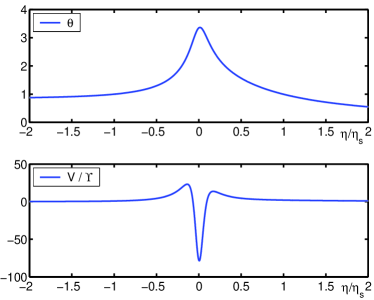
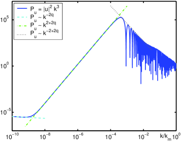
Figure 3: Case 1, $\theta_{1}\to\theta_{1}$, using $\tilde{\gamma}(\eta)=\iota(1-q)-1$. The $u$ potential (left) and spectrum, $P_{u}=|u|^{2}k^{3}$ (right) are shown for $q=5\cdot 10^{-2}$ and $\epsilon=10^{-2}$.

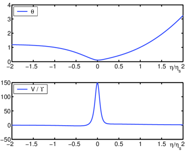
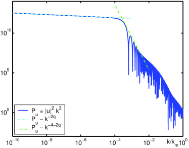
Figure 4: Case 2, $\theta_{1}\to\theta_{2}$, using $\tilde{\gamma}(\eta)=-\iota(2+q)+2$. The $u$ potential (left) and spectrum, $P_{u}=|u|^{2}k^{3}$ (right) are shown for $q=5\cdot 10^{-2}$ and $\epsilon=10^{-2}$.

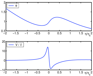
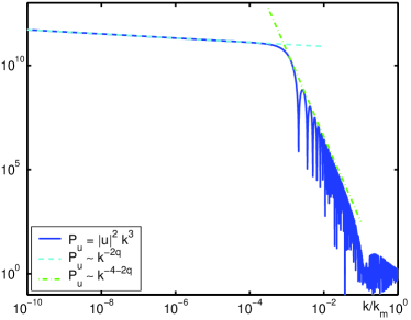
Figure 5: Case 3, $\theta_{2}\to\theta_{1}$, using $\tilde{\gamma}(\eta)=\iota(2+q)-1$. The $u$ potential (left) and spectrum, $P_{u}=|u|^{2}k^{3}$ (right) are shown for $q=5\cdot 10^{-2}$ and $\epsilon=10^{-2}$.

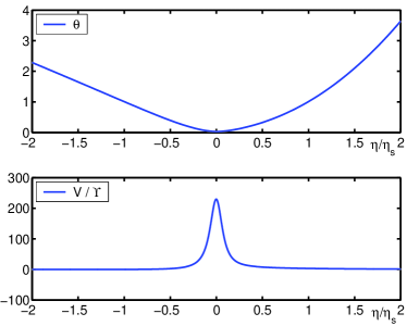
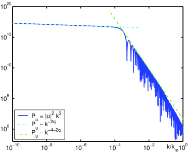
Figure 6: Case 4, $\theta_{2}\to\theta_{2}$, using $\tilde{\gamma}(\eta)=\iota(q-1)+2$. The $u$ potential (left) and spectrum, $P_{u}=|u|^{2}k^{3}$ (right) are shown for $q=5\cdot 10^{-2}$ and $\epsilon=10^{-2}$.

It is very encouraging that the numerical simulations produce a spectra with precisely the shape predicted analytically in the previous section. The spectra are evaluated at $\eta=\eta_{end}=10^{3}\eta_{s}$. As an example, we see that the kink predicted for case 1 is there in the figure and is found at the correct position,

$$k_{u}=\eta^{-1}\left({\eta\over\eta_{s}}\right)^{(2q-2)/(2q+1)}\simeq 8\times 10^{-9}\eta_{s}^{-1}\simeq 10^{-9}k_{m}~{}.$$ (116)

One also sees that the spectrum has the correct sub-Hubble radius slope, $n_{sub}=n-4$ for scales $k>10^{-3}\eta_{s}^{-1}$ which have already entered the Hubble radius at $\eta_{end}$.

It is interesting to note that the cases 2 and 3 have roughly the same amplitude while the amplitude of case 4, which we expect to depend on the transition, is much higher.

It is important to investigate the stability of the spectral index $n=3+2q$ of case 1. To do this we have slightly modified the potential for this case in the following way:

1. For $\eta/\eta_{s}\in[-0.5,0.5]$, $V_{u}\to V_{u}+10^{-1}$,  [(1) in Fig. 7].

2. For $\eta/\eta_{s}\in[-0.5,0.5]$, $V_{u}\to V_{u}+10^{-3}$,  [(2) in Fig. 7].

3. For $\eta/\eta_{s}\in[-0.1,0.1]$, $V_{u}\to V_{u}+10^{-3}$,  [(3) in Fig. 7].

The result is shown in Fig 7. The plain curve represents the original case, $V_{u}=\theta_{1}^{\prime\prime}/\theta_{1}$. Adding a tiny constant $[\sim{\cal O}(10^{-3})]$ to this potential during about a tenth of the duration of the transition [curve (3)] already modifies significantly the amplification on super-Hubble scales and the final spectral index becomes $n=1-2q$. Analyzing the growing and decaying modes separately, we have seen that, due to the perturbation of the potential, a tiny portion of the growing mode during the pre-big-bang phase is converted into the growing mode during the radiation era. This is already sufficient for the latter to inherit the naively expected spectrum $n=1-2q$ like the other cases. The later we evaluate the spectrum the more pronounced becomes the difference from the “pure case 1” spectrum. We expect that at very late times, hence very large scales, extremely small differences from the pure case 1 potential will have lead to a scale invariant spectrum. We have also tested smooth modifications of the potential, like $V_{u}\to V_{u}+10^{-3}\exp[-10^{2}(\eta/\eta_{s})^{2}]$. They also lead to the same result. The spectra of the cases 2 to 4, however, are stable under small modifications of the corresponding potential.

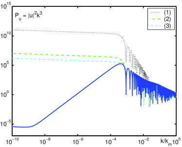
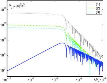
Figure 7: We draw the spectral distribution ${\cal P}_{u}=|u|^{2}k^{3}$ evaluated at $\eta/\eta_{s}=10^{3}$ (left) and $\eta/\eta_{s}=10^{5}$ (right) for $V_{u}$ of case 1 and the small modifications of the potential detailed in the text. Although modifying the potential during the transition may change $k_{m}$, we kept the same original value of $k_{m}$ for all spectra.

Finally, in Fig. 8 we show the corresponding spectra for dilaton-driven cosmology. The only difference to the previous simulations is that we set $q=1/2$ in this model which, in the Einstein frame, is a contracting universe with a scalar field with vanishing potential. Again we obtain precisely the spectra expected according to the arguments of the previous section.

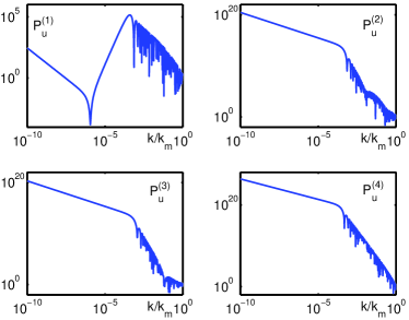
Figure 8: We illustrate the spectral distribution ${\cal P}_{u}^{(i)}=|u|^{2}k^{3}$ (case $i=1-4$) as a function of the rescaled comoving wave number $k/k_{m}$ The parameters for the simulations are $\epsilon=10^{-2}$, $q=0.5$ and the spectral distributions are evaluated in the radiation era $\eta/\eta_{s}=10^{3}$.

IV.3 A regular transition in the perturbation variable $v$

In this section we repeat the analysis presented above for the case of a regular equation for the variable $v$. Since the procedure is very close to the one presented above, we can be brief here. We again assume that there exists a regular potential $V_{v}$ such that

$$v^{\prime\prime}+(k^{2}\Upsilon-V_{v})v=0~{}.$$ (117)

In the case of a pure power law scale factor, $a=|\eta/\eta_{s}|^{q}$, we have $V_{v}=q(q-1)/\eta^{2}=z^{\prime\prime}/z$ where $z$ is either $z_{1}=a$ or $z_{2}=a\int a^{-2}d\eta$. To regularize the $v$ equation during the transition era we use our interpolation functions $\iota$, $\tilde{\gamma}$ and $\Upsilon$ [see Eqs. (109), (111) and (112), respectively] and impose

$$z(\eta)=\left[\left(\eta/\eta_{s}\right)^{2}+\epsilon\right]^{\tilde{\gamma}/2}~{}.$$ (118)

To reproduce the four cases for $v$, we make the following choices:

$$\tilde{\gamma}(\eta)=\left\{\begin{array}[]{rccrcr}\iota(q-1)+1&\mbox{ (case 1: }&z_{1}\to z_{1},&q&\to&1)~{},\\ \iota q&\mbox{ (case 2: }&z_{1}\to z_{2},&q&\to&0)~{},\\ -\iota q+1&\mbox{ (case 3: }&z_{2}\to z_{1},&1-q&\to&1)~{},\\ \iota(1-q)&\mbox{ (case 4: }&z_{2}\to z_{2},&1-q&\to&0)~{}.\end{array}\right.$$ (119)

The resulting spectra are shown in Fig. 9.

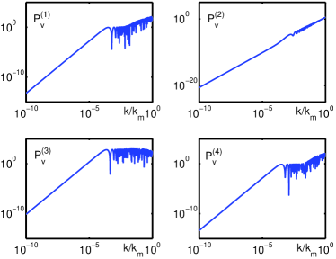
Figure 9: We illustrate the spectral distribution ${\cal P}_{v}^{(i)}=|v|^{2}k^{3}$ (case $i=1-4$) as a function of the rescaled comoving wave number $k/k_{m}$. The parameters for the simulations are $\epsilon=10^{-2}$, $q=5\cdot 10^{-2}$ and the spectral distributions are evaluated in the radiation era at $\eta/\eta_{s}=10^{3}$.

Again the spectra are in very good agreement with those obtained with our theoretical arguments. This gives us confidence that we really understand what is going on. During the radiation era $v$ grows like $\eta$ on super-Hubble scales. Inside the Hubble radius the amplitude of $v$ remains constant and it begins to oscillate. Neglecting the oscillations, we therefore expect for the cases 1, 3 and 4

$$P_{v}\propto k^{2+2q}(\eta_{s}/\eta+k\eta)^{-2},$$ (120)

leading to the observed flat spectrum inside the Hubble radius. The spectrum of case 2 turns from $P_{v}\propto k^{4-2q}$ to $P_{v}\propto k^{2-2q}$ inside the Hubble radius. For $k\,\raise 1.72218pt\hbox{$>$}\kern-6.99997pt\lower 2.6694pt\hbox{$\sim$}\,10^{-3}k_{m}$ the spectrum is not very reliable, since it is influenced by the details of the transition. The kink in the spectral distribution expected for case $2$ is not well visible since $q=5\cdot 10^{-2}$ is very small (see the argument on the previous section). We have repeated this case for a larger value, $q=0.3$, where the kink can now be seen, as illustrated in Fig. 10. Finally, note that case 2 for $v$ is unstable in the same sense as case 1 for $u$ and therefore probably irrelevant.

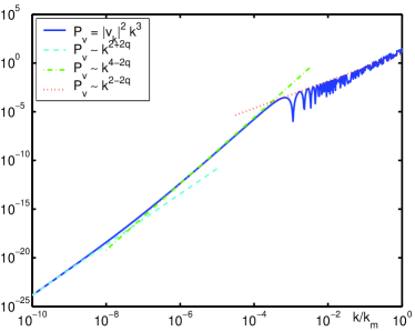
Figure 10: We illustrate the spectral distribution ${\cal P}_{v}=|v|^{2}k^{3}$ of case 2 as a function of the rescaled comoving wave number $k/k_{m}$. The parameters for the simulations are $\epsilon=10^{-2}$, $q=0.3$ and the spectral distribution is evaluated in the radiation era at $\eta/\eta_{s}=10^{3}$. We confront our predictions for the spectral slopes: above and below the kink at $k_{v_{1}}/k_{m}\sim 10^{-8}-10^{-7}$, the decaying mode is still dominant on scales $k\leqslant k_{v_{1}}$.

V Discussion

V.1 Which variable, $u$ or $v$?

We have shown that during a contracting (or inflationary for $q<0$) phase where the scale factor evolves according to a power law, $a\propto|\eta|^{q}$ with $q>-1/2$, the variables $u$ and $v$ acquire a spectral index

$$P_{u}\propto k^{-2q}~{},\quad~{}n_{u}=1-2q~{},$$ (121)

$$P_{v}\propto k^{2+2q}~{},\quad n_{v}=3+2q\quad\mbox{ if }q\leqslant 1/2~{},$$ (122)

$$P_{v}\propto k^{4-2q}~{},\quad n_{v}=5-2q\quad\mbox{ if }q\geqslant 1/2~{}.$$ (123)

We have also shown that, if the corresponding variable transits regularly into the radiation era, the spectrum is inherited in this era. But, during the radiation era and on large scales ($k\eta\ll 1$) $u$ and $v$ are simply related to $\Psi$, via [see Eqs. (10), (20) and (22)]

$$\Psi=\left({M_{s}\over M_{P}}\right)\sqrt{2}a^{-2}u=-{\sqrt{6}\over 9}M_{P}^{-1}a^{-1}v~{},$$ (124)

which therefore has the same spectrum as both $u$ and $v$. The only possible resolution of this contradiction is that either $u$ or $v$ is not regular at the transition and makes a strongly $k$-dependent jump. But which one?

We do not know the general answer to this question. It is quite likely to be model dependent. Nevertheless, we are able to prove the following statement.

Theorem. If the perturbed metric remains regular during the transition and if its evolution can be described by a second order differential equation for the Bardeen potential $\Psi$, then a regular $u$-variable which satisfies an equation of the form (11) can be found.

Proof. If the metric perturbations are regular, the Bardeen potential which is in general given by (see, e.g. Durrer:1993db )

$$\Psi=A+k^{-1}{\cal H}(B-k^{-1}H_{T}^{\prime})+k^{-1}(B-k^{-1}H_{T}^{\prime})^{\prime}~{},$$ (125)

is regular too. Here (scalar) metric perturbations are parametrized with the four variables $A$, $B$, $H_{L}$ and $H_{T}$ via

$$ds^{2} = \left[-(1+2A)d\eta^{2}-i2B\hat{k}_{j}dx^{j}d\eta+\Big{\{}\Big{(}1+2H_{L}-\frac{2}{3}H_{T}\Big{)}\delta_{jm}\right.$$ (126)

$$\quad\left.+2H_{T}\hat{k}_{j}\hat{k}_{m}\Big{\}}dx^{j}dx^{m}\right]a^{2}e^{-i{\bf k\cdot x}}~{},$$

and $\hat{k}_{j}=k_{j}/k$.

During a period governed by general relativity (and in the absence of anisotropic stresses) the Bardeen potential satisfies an equation of the form

$$\Psi^{\prime\prime}+f(\eta)\Psi^{\prime}+\left[\Upsilon(\eta)k^{2}-g(\eta)\right]\Psi=0~{},$$ (127)

where $f$, $g$ and $\Upsilon$ are smooth functions. If the scale factor obeys a simple power law evolution, $a\propto|\eta|^{q}$, we have $f=2(1+q)/\eta$ and $g=0$. If $f$ and $g$ remain smooth during the transition, we can define

$$u=\exp\left({1\over 2}\int fd\eta\right)\Psi~{}.$$ (128)

As one easily verifies, this variable satisfies

$$u^{\prime\prime}+(\Upsilon k^{2}-V_{u})u=0$$ (129)

with

$$V_{u}=g+{1\over 2}f^{\prime}+{1\over 4}f^{2}~{}.$$ (130)

$V_{u}$ is well defined, smooth and bounded in any finite interval, so that the differential equation

$$\theta^{\prime\prime}=V_{u}\theta$$ (131)

has two well-defined solutions $\theta_{1}$ and $\theta_{2}$ which are the pump fields. Up to an irrelevant constant the so-defined variable $u$ coincides with the well known $u$ given in Eq. (11) in the asymptotic past $\eta\ll-\eta_{s}$ and in the asymptotic future $\eta\gg\eta_{s}$. Hence it is our regularized variable $u$. $\Box$

On the other hand, if $\zeta$ passes via a regular second order equation through the transition, the same theorem leads to a regular $v$-equation and hence to a spectral index $n=3+2q$ for $q\leqslant 1/2$.

This shows again that it is not possible for both $\Psi$ and $\zeta$ to pass through the transition regularly (if $-1/2<q$). This is consistent with the expressions Eq. (20) or Eq. (21) which relate $\zeta$ and $\Psi$. If these equations are also valid during the transition, $\zeta$ necessarily diverges if $\Psi$ is regular and vice versa since ${\cal H}$ and ${\cal H}^{\prime}-{\cal H}^{2}=aH^{\prime}$ have to pass through zero in a transition from contraction to expansion (see also Fig. 2). Of course these relations will in general be modified during the transition, but according to our results the modifications should be such that one of the two variables has to develop a singularity if the other is regular.

V.2 Amplitude of the perturbations

During contraction the Bardeen potential grows like $\Psi\propto|\eta|^{-(1+2q)}$ on super-Hubble scales. One actually has

$$|\Psi|^{2}k^{3}\simeq\left({M_{s}\over M_{P}}\right)^{2}\left|\frac{\eta}{\eta_{s}}\right|^{-(2+4q)}(k\eta_{s})^{-2q}\quad\mbox{ for }q\geqslant-1/2~{}.$$ (132)

Hence $\Psi$ may become much larger than $1$ for $k\ll 1/\eta_{s}$ and $|\eta|\sim\eta_{s}$. Does this imply that perturbation theory breaks down during the contraction phase? We show now that this is not the case for $q\leqslant 1$. First let us note that a quantity relevant to measure the deviation of the geometry from Friedmann is, for example, the Weyl curvature whose background component vanishes. It is well known (see, e.g. Durrer:1993db ) that the ratio between a typical component of the Weyl tensor to a typical component of the background Riemann tensor is given by $|C/R|\simeq(k\eta)^{2}\Psi$. The geometrical deviation away from Friedmann is thus of the order of

$$|C/R|^{2}k^{3}\simeq\left({M_{s}\over M_{P}}\right)^{2}\left|\frac{\eta}{\eta_{s}}\right|^{-4q}(k\eta_{s})^{2-2q}(k\eta)^{2}~{},$$ (133)

which is always much smaller than $1$ on super-Hubble scales for $-1/2\leqslant q\leqslant 1$ and $|\eta|\,\raise 1.72218pt\hbox{$>$}\kern-6.99997pt\lower 2.6694pt\hbox{$\sim$}\,\eta_{s}$. Only in a contracting universe with $q>1$ do the perturbations become large and hence perturbation theory becomes invalid.

To ensure that perturbations truly remain small, it is necessary to find a gauge in which all the metric perturbations are small. We show now that this is so in the off-diagonal gauge which also has been used in Brustein:1995kn for dilaton-driven string cosmology. This gauge is defined by $H_{T}=H_{L}=0$. According to Eq. (125), the Bardeen potential is then given by

$$\Psi=A+k^{-1}({\cal H}B+B^{\prime})~{}.$$ (134)

The $(ij)$ Einstein equation implies (see e.g. Durrer:1993db )

$$\Psi=A+k^{-1}({\cal H}B+B^{\prime})=-k^{-1}{\cal H}B~{}.$$ (135)

Before the transition, the Bardeen potential is given by

$$\Psi={\sqrt{{\cal H}^{2}-{\cal H}^{\prime}}\over M_{P}a}u=\sqrt{q(q+1)}\left({M_{s}\over M_{P}}\right)\left|{\eta_{s}\over\eta}\right|^{1+q}u~{}.$$ (136)

On super-Hubble scales this gives for $q>-1/2$, using Eq. (16),

$$|\Psi| \simeq \sqrt{q(q+1)}\left({M_{s}\over M_{P}}\right)k^{-3/2}(k\eta_{s})^{-q}\left|{\eta_{s}\over\eta}\right|^{1+2q}\big{[}1+{\cal O}(|k\eta|^{\sigma})\big{]}$$ (137)

with $$\sigma=\min(2q+1,2).$$

The exponent $\sigma>0$ (for $q>-1/2$) of the first correction to the dominant term can be obtained by expanding the Hankel function solution given in Eqs. (15,10). With Eq. (135) we then obtain

$$B \simeq \sqrt{q+1\over q}\left({M_{s}\over M_{P}}\right)k^{-3/2}(k\eta_{s})^{1-q}\left|{\eta_{s}\over\eta}\right|^{2q}\left[1+{\cal O}\left(|k\eta|^{\sigma}\right)\right]~{},$$ (138)

$$k^{3}|B|^{2} \simeq \left({M_{s}\over M_{P}}\right)^{2}|k\eta|^{2-2q}\left|{\eta_{s}\over\eta}\right|^{2+2q}~{},$$ (139)

which remains small on super horizon scales, $|k\eta|<1$ during the entire contraction phase, $\eta\leqslant-\eta_{s}$, for $q\leqslant 1$ . From $A=-k^{-1}(2{\cal H}B+B^{\prime})$ and Eq. (138) we find that ${\cal O}(A)={\cal O}(|k\eta|^{\sigma-1}B)$, hence

$$k^{3}|A|^{2}\simeq\left({M_{s}\over M_{P}}\right)^{2}|k\eta|^{2\sigma-2q}\left|{\eta_{s}\over\eta}\right|^{2+2q}~{}.$$ (140)

Inserting the value of $\sigma$ given above this becomes

$$k^{3}|A|^{2}\simeq\left\{\begin{array}[]{ll}\left({M_{s}\over M_{P}}\right)^{2}|k\eta|^{2+2q}\left|{\eta_{s}\over\eta}\right|^{2+2q}&\mbox{ for }-1/2<q\leqslant 1/2~{},\\ \left({M_{s}\over M_{P}}\right)^{2}|k\eta|^{4-2q}\left|{\eta_{s}\over\eta}\right|^{2+2q}&\mbox{ for }1/2\leqslant q~{}.\\ \end{array}\right.$$ (141)

With $B$ also $A$ remains small on super-Hubble scales as long as $q\leqslant 1$ (actually $A$ remains small even for $1<q\leqslant 2$). In this treatment we have neglected the logarithm corrections which are present for $q=1/2$. Note that it is highly non-trivial that $A$ remains small. This is due to the fact that $B\propto a^{-2}(1+{\cal O}|k\eta|^{\sigma})$ and hence the lowest order contribution to $A$ cancels.

Since the generic form of the perturbed Einstein equations is ${\cal O}[h+(k\eta)h+(k\eta)^{2}h]={\cal O}(\Delta)$ where $h$ and $\Delta$ are typical metric and matter perturbation variables, respectively (see, e.g. Durrer:1993db ), the matter perturbation variables in this gauge are also small on super-Hubble scales. More precisely we find from the perturbed Einstein equations in the off-diagonal gauge

$$\delta = -{9\over 2}A+{3\over 2}(k/{\cal H})B\simeq{\cal O}(A)~{},$$ (142)

$$\xi = {2k\over 3{\cal H}(1+w)}A+B\simeq B~{},$$ (143)

$$\pi_{L} = {2\over 3w}\left[{\cal H}^{-1}A^{\prime}+{\cal H}^{-2}(2{\cal H}^{\prime}+{\cal H}^{2})A\right]\simeq{\cal O}(A)~{}.$$ (144)

Here $\delta$ and $\pi_{L}$ are the density and pressure perturbations, respectively, and $i(\rho+P)\hat{k}_{j}\xi$ is the scalar perturbation of the energy flux, $T^{0}_{j}$. To obtain the above results we have used the fact that $a\propto|\eta|^{q}$ obeys a simple power law and $B\propto|\eta|^{-2q}$ as well as $A\propto|\eta|^{\max(0,1-2q)}$.

Our result that the perturbations remain small hold as long as $\eta<-\eta_{s}$, which is the epoch when we expect higher order curvature corrections to become important. Typically we would expect this to be around the Planck scale. After that, what will happen depends on the specific model considered.

VI Conclusion

In this work we have analyzed the behavior of scalar perturbations in a transition from a contracting to an expanding Friedmann universe. We have shown that, if the perturbation equation during the transition can be formulated as second order equations for either $\Psi$ or $\zeta$, regular variables $u$ or $v$, respectively, can be found. The resulting spectral index in the late radiation dominated universe depends on which of these two variables passes regularly, and there are no stable cases where both $u$ and $v$ (equivalently $\Psi$ and $\zeta$), are regular during the transition.

The resulting spectral index $n$ is given by

$$n=\left\{\begin{array}[]{ll}1-2q&\mbox{if $\Psi$ is regular},\\ 3+2q&\mbox{if $\zeta$ is regular and $q\leqslant 1/2$},\\ 5-2q&\mbox{if $\zeta$ is regular and $q>1/2$}.\end{array}\right.$$ (145)

Our numerical results for the spectral index obtained from a simple toy model are in perfect agreement with the more general arguments of Sec. III.

This result remains valid in an inflationary universe with $-1/2<q<0$, but has never raised any attention since such models cannot produce the observed scale invariant spectrum and require $w<-1$. For $q<-1/2$ both variables $u$ and $v$ lead to the same spectral index $n=3+2q$. Therefore, this problem has not been noticed in works on standard inflationary models where $q\simeq-1$.

We have also shown that, as long as $q\leqslant 1$, and we are in a regime where corrections to the equations of motion can be ignored, perturbations remain small during contraction in the sense that there exists a gauge in which all the metric and matter perturbation variables are small.

We have also argued that the $v$ equation derived from string corrections in Cartier:2001is has to be considered as a toy model, since higher order corrections cannot be neglected in this case.

Our findings explain that all the literature based on the variable $v$ predicts $n=3+2q$, see especially Refs. Cartier:2001is and Tsujikawa:2002qc , while when mainly working with $u$ one finds that the spectral index $n=3+2q$ is highly unstable and one typically expects $n=1-2q$.

This work has the following important implications.

• If it can be shown that in the ekpyrotic model Khoury:2001wf ; Khoury:2001zk where $0<q\ll 1$ the Bardeen potential passes regularly through the transition, this model leads to a nearly scale invariant spectrum with $n=1-2q$.

• In dilaton-driven string cosmology we have the opposite situation. There, $q=1/2$ and it has generically been assumed that $\zeta$ passes regularly through the transition. This has been shown to be true to first order in $\alpha^{\prime}$ in Cartier:2001is . Then the spectral index is $n=3+2q=4$ leading to a very blue spectrum of highly suppressed perturbation Brustein:1995kn . In this case, a scale invariant spectrum of adiabatic perturbations of the axion field can be obtained via the “curvaton mechanism” Bozza:2002fp . If, however, $\Psi$ would be regular, a red spectrum with $n=1-2q$ is obtained. This would mean a fatal blow for dilaton-driven string cosmology, since the perturbations then become very large in the radiation dominated era: Since the Bardeen potential is large at the end of the pre-big-bang phase and since $|C/R|\simeq(k\eta)^{2}|\Psi|\simeq|\Psi|$ at Hubble crossing, the Weyl tensor becomes larger than the background Riemann tensor at Hubble crossing. Even though the Weyl tensor has constant amplitude on super-Hubble scales, the decay of the Riemann tensor during expansion leads to a huge increase in the ratio $|C/R|$. This problem only affects red spectra, since for blue spectra $|C/R|$ at Hubble crossing is always smaller than $|\Psi(k_{\max})|\simeq|C/R|$ evaluated at $\eta=-\eta_{s}$ for $k=k_{\max}$.

Even though we cannot establish from first principles in this work which spectrum dilaton-driven string cosmology or the ekpyrotic model have, we nevertheless have formulated sufficient (but maybe not necessary) conditions on the transition which would allow such a decision.

References

- (1) J. Khoury, B. A. Ovrut, P. J. Steinhardt, and N. Turok, Phys. Rev. D 66, 046005 (2002), [hep-th/0109050].
- (2) R. Durrer and F. Vernizzi, Phys. Rev. D 66, 083503 (2002), [hep-ph/0203275].
- (3) P. Peter and N. Pinto-Neto, Phys. Rev. D 66, 063509 (2002), [hep-th/0203013].
- (4) J. Khoury, B. A. Ovrut, P. J. Steinhardt, and N. Turok, Phys. Rev. D 64, 123522 (2001), [hep-th/0103239].
- (5) R. Brandenberger and F. Finelli, JHEP 11, 056 (2001), [hep-th/0109004].
- (6) D. H. Lyth, Phys. Lett. B 524, 1 (2002), [hep-ph/0106153].
- (7) J.-c. Hwang, Phys. Rev. D 65, 063514 (2002), [astro-ph/0109045].
- (8) S. Gratton, J. Khoury, P. J. Steinhardt, and N. Turok, (2003), [astro-ph/0301395].
- (9) I. Antoniadis, J. Rizos, and K. Tamvakis, Nucl. Phys. B415, 497 (1994), [hep-th/9305025].
- (10) R. Brustein and R. Madden, Phys. Rev. D 57, 712 (1998), [hep-th/9708046].
- (11) S. Foffa, M. Maggiore, and R. Sturani, Nucl. Phys. B552, 395 (1999), [hep-th/9903008].
- (12) C. Cartier, E. J. Copeland, and R. Madden, JHEP 01, 035 (2000), [hep-th/9910169].
- (13) C. Cartier, J. C. Hwang, and E. J. Copeland, Phys. Rev. D 64, 103504 (2001), [astro-ph/0106197].
- (14) S. Tsujikawa, R. Brandenberger, and F. Finelli, Phys. Rev. D 66, 083513 (2002), [hep-th/0207228].
- (15) F. Finelli and R. Brandenberger, Phys. Rev. D 65, 103522 (2002), [hep-th/0112249].
- (16) V. F. Mukhanov, H. A. Feldman, and R. H. Brandenberger, Phys. Rept. 215, 203 (1992).
- (17) R. Durrer, Fund. Cos. Phys. 15, 209 (1994), [astro-ph/9311041].
- (18) D. H. Lyth, Phys. Rev. D 31, 1792 (1985).
- (19) G. Veneziano, Phys. Lett. B 265, 287 (1991), [CERN-TH.6077/91].
- (20) M. Gasperini and G. Veneziano, Phys. Rep. 373, 1 (2003), [hep-th/0207130].
- (21) R. Brustein, M. Gasperini, M. Giovannini, V. F. Mukhanov, and G. Veneziano, Phys. Rev. D 51, 6744 (1995), [hep-th/9501066].
- (22) N. Deruelle and V. F. Mukhanov, Phys. Rev. D 52, 5549 (1995), [gr-qc/9503050].
- (23) D. N. Page, Class. Quantum Grav. 1, 417 (1984).
- (24) D. Wands, Phys. Rev. D 60, 023507 (1999), [gr-qc/9809062].
- (25) R. Brustein, M. Gasperini, and G. Veneziano, Phys. Lett. B 431, 277 (1998), [hep-th/9803018].
- (26) I. P. C. Heard and D. Wands, Class. Quant. Grav. 19, 5435 (2002), [gr-qc/0206085].
- (27) V. Bozza, M. Gasperini, M. Giovannini, and G. Veneziano, Phys. Lett. B 543, 14 (2002), [hep-ph/0206131].