Color Reflection Invariance and Monopole Condensation in QCD

Abstract:

We review the quantum instability of the Savvidy-Nielsen-Olesen (SNO) vacuum of the one-loop effective action of $SU(2)$ QCD, and point out a critical defect in the calculation of the functional determinant of the gluon loop in the SNO effective action. We prove that the gauge invariance, in particular the color reflection invariance, exclude the unstable tachyonic modes from the gluon loop integral. This guarantees the stability of the magnetic condensation in QCD.

1 Introduction

The confinement problem in quantum chromodynamics (QCD) is probably one of the most challenging problems in theoretical physics. It has long been argued that the confinement in QCD can be triggered by the monopole condensation [1, 2]. Indeed, if one assumes monopole condensation, one can easily argue that the ensuing dual Meissner effect could guarantee the confinement of color [1, 2, 3]. But it has been extremely difficult to prove the monopole condensation in QCD. Although the monopole condensation has been established in a supersymmetric QCD [4], a satisfactory theoretical proof of the desired monopole condensation in the conventional QCD has remained elusive.

A natural way to establish the monopole condensation in QCD is to demonstrate that the quantum fluctuation triggers a phase transition through the dimensional transmutation known as the Coleman-Weinberg mechanism [5], by generating a non-trivial vacuum which can be identified as a monopole condensation. Coleman and Weinberg have demonstrated that the quantum effect could trigger a phase transition in massless scalar QED with a quartic self-interaction of scalar electrons, by showing that the one-loop effective action generates a condensation of scalar electrons which defines a non-trivial new vacuum. To prove the monopole condensation, one need to demonstrate such a phase transition in QCD. There have been many attempts to do so with the one-loop effective action of QCD using the background field method [6, 7, 8]. Savvidy has first calculated the effective action of $SU(2)$ QCD in the presence of an ad hoc color magnetic background, and has almost “proved” the magnetic condensation in QCD. In particular, he showed that the quantum effective potential obtained from the real part of the one-loop effective action has the minimum at a non-vanishing magnetic background [6]. This is exactly what everybody was looking for. Unfortunately, this calculation was repeated by Nielsen and Olesen, who showed that the magnetic background generates an extra imaginary part in the effective action which induces the pair-creation of the gluons and thus destablizes the magnetic condensation [7]. This instability of the “Savvidy-Nielsen-Olesen (SNO) vacuum” has never been seriously challenged, and destroyed the hope to establish the monopole condensation in QCD with the effective action [8].

A few years ago, however, there has been a new attempt to calculate the one-loop effective action of QCD with a gauge independent separation of the non-Abelian monopole background from the quantum field [9]. Remarkably, in this calculation the effective action has been shown to produce no imaginary part in the presence of the monopole background, but a negative imaginary part in the presence of the pure color electric background. This implies that in QCD the non-Abelian monopole background produces a stable monopole condensation, but the color electric background becomes unstable by generating a pair annhilation of the valence gluon at one-loop level. The new result sharply contradicts with the earlier results, in particular on the stability of the monopole condensation. This has resurrected the old controversy on the stability of monopole condensation.

To resolve the controversy it is important to understand the origin of the instability of the SNO vacuum. It is well-known that the energy of a charged vector field moving around a constant magnetic field depends on the spin orientation of the vector field, and when the spin is anti-parallel to the magnetic field, the zeroth Landau level has a negative energy. Because of this the functional determinant of the gluon loop in the SNO magnetic background necessarily contains negative eigenvalues which create a severe infra-red divergence in the effective action [7]. And, when one regularizes this divergence with the $\zeta$-function regularization, one obtains the well-known imaginary component in the effective action which destablizes the magnetic condensation. This shows that the instability of the SNO vacuum originates from the the negative eigenvalues of the functional determinant. Since the existence of the negative eigenvalues is so obvious, the instability of the SNO vacuum has become the prevailing view which nobody has dared to challenge [7, 8].

This popular view, however, is not without defect. To see this notice that the eigenfuctions corresponding to the negative eigenvalues describes the tachyons which violate the causality and thus become unphysical. This implies that one should exclude these tachyons in the calculation of the effective action. But the standard $\zeta$-function regularization fails to remove the contribution of the tachyonic eigenstates because it is insensitive to causality. On the other hand, if we adopt the infra-red regularization which respects the causality, the resulting effective action no longer has the imaginary part [9]. But since the $\zeta$-function regularization has worked so well in quantum field theory, there seems no compelling reason why it should not work in QCD. So we need an independent argument which can support the stability of the magnetic condensation in QCD.

One way to check the stability of the magnetic condensation is to calculate the imaginary part of the one-loop effective action with a perturbative method. This idea was first proposed by Schanbacher, but has never been taken seriously till recently [10]. This is understandable because the monopole condesnation is supposed to be a non-perturbative effect, and it is highly unlikely that one can calculate a non-perturbative effect with a perturbative method. The massless gauge theories, however, have a very unique feature that the imaginary part of the one-loop effective action is propotional to $g^{2}$, where $g$ is the coupling constant. This is true in both QCD [7, 8] and massless QED [11, 12]. This enables us to calculate the imaginary part of the effective action with a perturbative method. Remarkably the recent perturbative calculation has confirmed that the effective action should have no imaginary part in the magnetic background [13]. This might sound surprising but could really have been expected, because the perturbative calculation is based on the causality which naturally excludes the contribution of tachyonic eigenstates in the calculation of the effective action.

The perturbative confirmation of the infra-red regularization by causality should settle the controversy on the stability of the monopole condensation. But this does not settle the controversy completely. There are more questions to be answered. The perturbative calculation does tell that the tachyonic modes should be excluded in the calculation of the effective action, because they violate the causality. If so, they should have been excluded in the calculation of the functional determinant. Unfortunately the perturbative calculation does not tell exactly what went wrong in the earlier calculation of the SNO effective action. In particular, it does not tell why one could not exclude the tachyonic modes in the calculation of the functional determinant. Considering the fact that the monopole condensation is such an important issue for the confinement in QCD, one can not easily dismiss the instability of the SNO vacuum before one figures out exactly how one can remove them from the functional determinant. Since both the infra-red regularization by causality and the perturbative calculation are based on the causality principle, it would be more convincing if one could show this with an independent principle.

Fortunately we do have an independent principle, the principle of gauge invariance, which allows us to demonstrate this. The SNO vacuum is not gauge invariant, and the instability of the SNO vacuum has been attributed to this defect. To cure this defect Nielsen and Olesen have introduced “the Copenhagen vacuum” which is made of gauge invariant combination of blockwise randomly oriented color magnetic fields, and suggested that such a gauge invariant vacuum could generate a stable magnetic condensation [7]. But this Copenhagen vacuum, although conceptually appealing, has not been so useful to prove the monopole condensation.

The purpose of this paper is to show that a proper implementation of the gauge invariance in the calculation of the functional determinant of the gluon loop excludes the unstable tachyonic modes, and thus naturally restore the stability of the magnetic background. This suggests that it is the incorrect calculation of the functional determinant, not the $\zeta$-function regularization, which causes the instability of the SNO vacuum. This means that tachyons should not have been there in the first place. They were there to create a mirage, not physical states. In the absence of the tachyons, of course, there is no instability of the SNO vacuum. This vindicates the $\zeta$-function regularization. It is simply too honest to correct the incorrect calculation of the functional determinant.

In the old approach Savvidy starts from an ad hoc magnetic background which is not gauge invariant [6, 7]. Because of this the functional determinant of the gluon loop contains the tachyonic eigenstates when the gluon spin is anti-parallel to the magnetic field, which in turn develops an imaginary part in the effective action and destabilizes the SNO vacuum. In the following, however, we show that the spin polarization of the gluon is not a gauge independent concept. The reason is that one can change the direction of the magnetic field with a simple gauge transformation, so that the spin flip of the gluon corresponds to a gauge transformation. This means that the gauge invariant part of the functional determinant should not contain any negative eigenvalue. This tells that, if we impose the gauge invariance properly, the instability of the SNO background should disappear.

In our approach we start from a gauge invariant non-Abelian monopole background from the beginning [9, 13]. This precludes the tachyonic eigenstates to enter in the calculation of the effective action. In this paper we show that a natural way to make the monopole background gauge invariant is to impose the color reflection invariance to the vacuum, and show how this color reflection invariance removes the contribution of tachyonic modes in the functional determinant of the gluon loop. In fact we show that this gauge invariant calculation produces exactly the same effective action we obtain with the infra-red regularization by causality.

The paper is organized as follows. In Section II we review the background field method to calculate the quantum effective action of QCD. In Section III we rederive the old SNO effective action, and discuss how the $\zeta$-function regularization creates the instability of the SNO vacuum. In Section IV we discuss the gauge independent separation of the monopole background from the quantum fluctuation, and compare the monopole background with the gauge dependent SNO background. In Section V we review the infra-red regularization by causality, and show how the infra-red regularization by causality generates a stable monopole condensation in QCD. In Section VI we briefly discuss the perturbative calculation of the imaginary part of the QCD effective action, and show how the perturbative calculation endorses the the infra-red regularization by causality. In Section VII we review the color reflection invarince in QCD, and show how the reflection invarince excludes the tachyonic modes from the functional determinant of the gluon loop and assures the stability of the monopole condensation. In Section VIII we discuss the physical meaning of our analysis, in particular the color reflection invarince, in connection with the confinement in QCD.

2 Background Field Method: A Review

In this section we review the background field method [14, 15] to obtain the one-loop effective action of QCD, and derive the integral expression of the QCD effective action. For simplicity we will concentrate on $SU(2)$ QCD in this paper.

To obtain the one-loop effective action one must first divide the gauge potential $\vec{A}_{\mu}$ into two parts, the slow-varying classical background $\vec{B}_{\mu}$ and the fluctuating quantum part $\vec{Q}_{\mu}$,

$$\vec{A}_{\mu}=\vec{B}_{\mu}+\vec{Q}_{\mu},$$ (1)

and integrate out the quantum part with a functional integration. To do this remember that (1) allows two types of gauge transformations, the background gauge transformation described by

$$\delta\vec{B}_{\mu}=\displaystyle\frac{1}{g}\bar{D}_{\mu}\vec{\alpha},~{}~{}~{}~{}~{}\delta\vec{Q}_{\mu}=-\vec{\alpha}\times\vec{Q}_{\mu},$$

$$\bar{D}_{\mu}=\partial_{\mu}+g\vec{B}_{\mu}\times,$$ (2)

and the physical gauge transformation described by

$$\delta\vec{B}_{\mu}=0,~{}~{}~{}~{}~{}\delta\vec{Q}_{\mu}=\displaystyle\frac{1}{g}D_{\mu}\vec{\alpha},$$ (3)

where $\vec{\alpha}$ is an infinitesimal gauge parameter. Notice that both (2) and (3) satisfy

$$\delta\vec{A}_{\mu}=\displaystyle\frac{1}{g}D_{\mu}\vec{\alpha}.$$ (4)

To integrate out the quantum field one may impose the following gauge condition to the quantum fields,

$$\vec{F}=\bar{D}_{\mu}\vec{Q}_{\mu}=0,$$

$${\cal L}_{gf}=-\displaystyle\frac{1}{2\xi}(\bar{D}_{\mu}\vec{Q}_{\mu})^{2}.$$ (5)

The corresponding Faddeev-Popov determinant is given by

$$M^{ab}_{FP}=\displaystyle\frac{\delta F^{a}}{\delta\alpha^{b}}=(\bar{D}_{\mu}D_{\mu})^{ab}.$$ (6)

With this gauge fixing the effective action takes the following form,

$$\exp~{}\Big{[}iS_{eff}(\vec{B}_{\mu})\Big{]}=\displaystyle\frac{}{}\int{\cal D}\vec{Q}_{\mu}{\cal D}\vec{c}~{}{\cal D}\vec{c}^{~{}*}\exp\Big{\{}~{}i\displaystyle\frac{}{}\int\Big{[}-\displaystyle\frac{1}{4}\vec{G}_{\mu\nu}^{2}-\displaystyle\frac{1}{4}(\bar{D}_{\mu}\vec{Q}_{\nu}-\bar{D}_{\nu}\vec{Q}_{\mu})^{2}$$

$$-\displaystyle\frac{g}{2}\vec{G}_{\mu\nu}\cdot(\vec{Q}_{\mu}\times\vec{Q}_{\nu})-\displaystyle\frac{g^{2}}{4}(\vec{Q}_{\mu}\times\vec{Q}_{\nu})^{2}+\vec{c}^{~{}*}\bar{D}_{\mu}D_{\mu}\vec{c}-\frac{1}{2\xi}(\bar{D}_{\mu}\vec{Q}_{\mu})^{2}\Big{]}d^{4}x\Big{\}},$$ (7)

where $\vec{c}$ and ${\vec{c}}^{~{}*}$ are the ghost fields. Notice that the effective action (7) is explicitly invariant under the background gauge transformation (2) which involves only $\vec{B}_{\mu}$, if we add the following gauge transformation of the ghost fields to (2),

$$\delta\vec{c}=-\alpha\times\vec{c},~{}~{}~{}~{}~{}\delta\vec{c}^{~{}*}=-\alpha\times\vec{c}^{~{}*}.$$ (8)

This guarantees the gauge invariance of the resulting effective action.

The gluon loop and the ghost loop integrals give the following functional deteminants (at one-loop level)

$${\rm Det}^{-\frac{1}{2}}K_{\mu\nu}^{ab}={\rm Det}^{-\frac{1}{2}}\Big{(}-g_{\mu\nu}\bar{D}^{2}_{ab}-2g\epsilon_{abc}G_{\mu\nu}^{c}\Big{)},$$

$${\rm Det}M_{ab}={\rm Det}\Big{(}-\bar{D}^{2}_{ab}\Big{)},$$ (9)

from which one has

$$\Delta S=\displaystyle\frac{i}{2}\ln{\rm Det}K-i\ln{\rm Det}M.$$ (10)

So the correct calculation of the determinants becomes crucial for us to obtain the effective action.

3 SNO Effective Action: A Review

Savvidy, and Nielsen and Olesen have chosen a covariantly constant color magnetic field as the classical background in their calculation of the effective action [6, 7, 8]

$$\vec{B}_{\mu}=\bar{B}_{\mu}\hat{n}_{0}=\displaystyle\frac{1}{2}\bar{H}_{\mu\nu}x_{\nu}\hat{n}_{0},~{}~{}~{}~{}~{}\vec{G}_{\mu\nu}=\bar{H}_{\mu\nu}\hat{n}_{0},$$

$$\bar{D}_{\mu}\vec{G}_{\mu\nu}=0,$$ (11)

where $\bar{H}_{\mu\nu}$ is a constant magnetic field and $\hat{n}_{0}$ is a constant unit isovector ($\hat{n}_{0}^{2}=1$). With the background, one can calculate the functional determinant (9). The calculation of the determinant amounts to the calculation of the eigenvalues of the determinant. Nielsen and Olesen have pointed out that this reduces to the calculation of the energy eigenvalues of a massless charged vector field $X_{\mu}$ in a constant external magnetic field $\bar{H}_{\mu\nu}$ [7],

$$E^{2}X_{\mu}=[-\bar{D}^{2}g_{\mu\nu}+\bar{D}_{\mu}\bar{D}_{\nu}+2ig\bar{H}_{\mu\nu}]X_{\nu}=0,$$

$$\bar{D}_{\mu}=\partial_{\mu}+ig\bar{B}_{\mu}.$$ (12)

Suppose the magnetic field is in $z$-direction. Then this has the well-known eigenvalues

$$E^{2}=2gH(n+\displaystyle\frac{1}{2})+k^{2}\pm 2gH,$$

$$H=\bar{H}_{12},$$ (13)

where $k$ is the momentum of the eigen-function in $z$-direction (the direction of the background magnetic field). Notice that the $\pm$ signature correspond to the spin $S_{3}=\pm 1$ of the charged vector field (in the direction of the magnetic field). So, when $n=0$, the eigen-functions with $S_{3}=-1$ have an imaginary energy when $k^{2}<gH$, and thus becomes tachyons which violate the causality. The eigenvalues of the functional determinant is shown in Fig. 1.

Figure 1: The eigenvalues of the functional determinant of the gluon loop. When the gluon spin is anti-parallel to the magnetic field ($S_{3}=-1$), the ground state (with $n=0$) becomes tachyonic when $k^{2}<gH$. Notice, however, that under the color reflection of ${\hat{n}}_{0}$ to $-{\hat{n}}_{0}$, the magnetic field changes its direction while the gluon spin remains the same. This means that the spin polarization direction of gluon with respect to the magnetic field is a gauge artifact, which tells that the gauge invariant functional determinant should not include the tachyonic state.

An important point here is that $\hat{n}_{0}$ can be rotated to $-\hat{n}_{0}$ by a gauge transformation. This means that one can change the direction of the magnetic field by a gauge transformation. And obviously the gauge transformation does not affect the gluon spin. This means that one can change the spin polarization direction of the gluon with respect to the magnetic field by a gauge transformation. But notice that the eigenstates with $S_{3}=-1$ changes to the eigenstates with $S_{3}=+1$ (and vise versa) under the gauge transformation. This tells that the eigenstates with $S_{3}=-1$ and $n=0$ are not invariant under the gauge transformation. This point will become very important when we make a gauge invariant calculation of the functional determinant in Section VII.

From (13) one obtains

$$\Delta S=i\ln{\rm Det}\Big{[}(-\bar{D}^{2}+2gH)(-\bar{D}^{2}-2gH)\Big{]},$$ (14)

and the integral expression of the effective action

$$\Delta{\cal L}=\displaystyle\frac{}{}\lim_{\epsilon\rightarrow 0}\displaystyle\frac{1}{16\pi^{2}}\int_{0}^{\infty}\displaystyle\frac{dt}{t^{2-\epsilon}}\displaystyle\frac{gH\mu^{2}}{\sinh(gHt/\mu^{2})}$$

$$\times\Big{[}\exp(-2gHt/\mu^{2})+\exp(+2gHt/\mu^{2})\Big{]},$$ (15)

where $\mu^{2}$ is a dimensional parameter.

The effective action has a severe infra-red divergence, and to perform the integral one has to regularize it first. Let us consider the popular $\zeta$-function regularization first. From the definition of the generalized $\zeta$-function [16]

$$\zeta(s,\lambda)=\displaystyle\frac{}{}\sum_{n=0}^{\infty}\displaystyle\frac{1}{(n+\lambda)^{s}}=\displaystyle\frac{1}{\Gamma(s)}\int_{0}^{\infty}\displaystyle\frac{x^{s-1}\exp(-\lambda x)}{1-\exp(-x)}dx,$$ (16)

we have

$$\Delta{\cal L}=\displaystyle\frac{}{}\lim_{\epsilon\rightarrow 0}\displaystyle\frac{\mu^{2}}{16\pi^{2}}\int_{0}^{\infty}\displaystyle\frac{dt}{t^{2-\epsilon}}\displaystyle\frac{gH}{\sinh(gHt/\mu^{2})}\Big{[}\exp(-2gHt/\mu^{2})+\exp(+2gHt/\mu^{2})\Big{]}$$

$$=\displaystyle\frac{}{}\lim_{\epsilon\rightarrow 0}\displaystyle\frac{\mu^{2}}{8\pi^{2}}gH\int_{0}^{\infty}\displaystyle\frac{dt}{t^{2-\epsilon}}\displaystyle\frac{\exp(-3gHt/\mu^{2})+\exp(+gHt/\mu^{2})}{1-\exp(-2gHt/\mu^{2})}$$

$$=\displaystyle\frac{}{}\lim_{\epsilon\rightarrow 0}\displaystyle\frac{(gH)^{2}}{4\pi^{2}}(\displaystyle\frac{2gH}{\mu^{2}})^{-\epsilon}\Gamma(\epsilon-1)\Big{[}\zeta(\epsilon-1,\displaystyle\frac{3}{2})+\zeta(\epsilon-1,-\displaystyle\frac{1}{2})\Big{]}$$

$$=\displaystyle\frac{}{}\lim_{\epsilon\rightarrow 0}\displaystyle\frac{(gH)^{2}}{4\pi^{2}}(1-\epsilon\ln\displaystyle\frac{2gH}{\mu^{2}})\big{(}\displaystyle\frac{1}{\epsilon}-\gamma+1\big{)}\Big{[}\big{(}\zeta(-1,\displaystyle\frac{3}{2})+\zeta(-1,-\displaystyle\frac{1}{2})\big{)}$$

$$+\epsilon\big{(}\zeta^{\prime}(-1,\displaystyle\frac{3}{2})+\zeta^{\prime}(-1,-\displaystyle\frac{1}{2})\big{)}\Big{]}$$

$$=\displaystyle\frac{11g^{2}}{48\pi^{2}}H^{2}\big{(}\displaystyle\frac{1}{\epsilon}-\gamma+1-\ln\displaystyle\frac{2gH}{\mu^{2}}\big{)}-\displaystyle\frac{g^{2}}{4\pi^{2}}H^{2}\big{(}2\zeta^{\prime}(-1,\displaystyle\frac{3}{2})-i\displaystyle\frac{\pi}{2}\big{)},$$ (17)

where $\zeta^{\prime}=\displaystyle\frac{d\zeta}{ds}(s,\lambda)$, and we have used the fact [16]

$$\zeta(-1,\displaystyle\frac{3}{2})=\zeta(-1,-\displaystyle\frac{1}{2})=-\displaystyle\frac{11}{24},~{}~{}~{}~{}~{}\zeta^{\prime}(-1,-\displaystyle\frac{1}{2})=\zeta^{\prime}(-1,\displaystyle\frac{3}{2})-i\displaystyle\frac{\pi}{2}.$$

So, with the ultra-violet regularization by modified minimal subtraction we arrive at the SNO effective action [6, 7, 8]

$${\cal L}_{eff}=-\displaystyle\frac{H^{2}}{2}-\displaystyle\frac{11g^{2}}{48\pi^{2}}H^{2}(\ln\displaystyle\frac{gH}{\mu^{2}}-c)+i\displaystyle\frac{g^{2}}{8\pi}H^{2},$$

$$c=1-\ln 2-\displaystyle\frac{24}{11}\zeta^{\prime}(-1,\frac{3}{2})=0.94556....$$ (18)

This contains the well-known imaginary part which destablizes the SNO vacuum. Observe that the imaginary part comes from the infra-red divergence which originates from the tachyonic eigenstates.

4 Monopole Background

Notice that the SNO background (11) is not gauge invariant. More seriously the separation of the SNO background from the quantum fluctuation is not gauge independent. So one is not sure whether the SNO effective action is gauge independent. This is a serious defect. To cure this defect we choose the monopole background given by [2, 3]

$$\vec{B}_{\mu}=\vec{C}_{\mu},~{}~{}~{}~{}~{}\vec{G}_{\mu\nu}=\vec{H}_{\mu\nu},$$

$$\vec{C}_{\mu}=-\displaystyle\frac{1}{g}\hat{n}\times\partial_{\mu}\hat{n},$$

$$\vec{H}_{\mu\nu}=\partial_{\mu}\vec{C}_{\nu}-\partial_{\nu}\vec{C}_{\mu}+g\vec{C}_{\mu}\times\vec{C}_{\nu}=-\displaystyle\frac{1}{g}\partial_{\mu}\hat{n}\times\partial_{\nu}\hat{n},$$ (19)

where $\hat{n}$ is a unit isovector ($\hat{n}^{2}=1$) which selects the color charge direction everywhere in space-time. The advantage of (19) over (11) is that in (11) one can not tell the origin of the magnetic background, whereas in (19) one can tell for sure that it comes exclusively from the non-Abelian monopole. More importantly, here the monopole background provides a gauge independent separation of the classical background from the quantum fluctuation.

To see this consider the gauge-independent decomposition of the gauge potential into the binding gluon $\hat{A}_{\mu}$ and the valence gluon ${\vec{X}}_{\mu}$ [2, 3],

$$\vec{A}_{\mu}=A_{\mu}\hat{n}-\displaystyle\frac{1}{g}\hat{n}\times\partial_{\mu}\hat{n}+{\vec{X}}_{\mu}=\hat{A}_{\mu}+{\vec{X}}_{\mu},$$

$$(A_{\mu}=\hat{n}\cdot\vec{A}_{\mu},~{}~{}~{}\hat{n}\cdot\vec{X}_{\mu}=0),$$ (20)

where $A_{\mu}$ is the “electric” potential. Notice that $\hat{A}_{\mu}$ is precisely the connection which leaves $\hat{n}$ invariant under parallel transport,

$${\hat{D}}_{\mu}\hat{n}=\partial_{\mu}\hat{n}+g{\hat{A}}_{\mu}\times\hat{n}=0.$$ (21)

Under the infinitesimal gauge transformation

$$\delta\hat{n}=-\vec{\alpha}\times\hat{n}\,,\,\,\,\,\delta{\vec{A}}_{\mu}=\displaystyle\frac{1}{g}D_{\mu}\vec{\alpha},$$ (22)

one has

$$\delta A_{\mu}=\displaystyle\frac{1}{g}\hat{n}\cdot\partial_{\mu}{\vec{\alpha}},\,\,\,\ \delta\hat{A}_{\mu}=\displaystyle\frac{1}{g}{\hat{D}}_{\mu}{\vec{\alpha}},$$

$$\hskip 34.14322pt\delta{\vec{X}}_{\mu}=-{\vec{\alpha}}\times{\vec{X}}_{\mu}.$$ (23)

This tells that $\hat{A}_{\mu}$ by itself describes an $SU(2)$ connection which enjoys the full $SU(2)$ gauge degrees of freedom. Furthermore $\vec{X}_{\mu}$ forms a gauge covariant vector field under the gauge transformation. This allows us to view QCD as the restricted gauge theory made of the binding gluon which has the valence gluon as the gauge covariant colored source. But what is really remarkable is that the decomposition is gauge independent. Once the gauge covariant topological field $\hat{n}$ is chosen, the decomposition follows automatically, regardless of the choice of gauge [2, 3].

Remember that $\hat{A}_{\mu}$ retains all the essential topological characteristics of the original non-Abelian potential. First, $\hat{n}$ defines $\pi_{2}(S^{2})$ which describes the non-Abelian monopoles. Indeed, it is well-known that $\vec{C}_{\mu}$ with ${\hat{n}}=\hat{r}$ describes precisely the Wu-Yang monopole [17, 18]. Secondly, it characterizes the Hopf invariant $\pi_{3}(S^{2})\simeq\pi_{3}(S^{3})$ which describes the topologically distinct vacua. So the topologically distinct vacua can be described exclusively by $\hat{n}$ [19, 20]. Furthermore $\hat{A}_{\mu}$ has a dual structure,

$$\hat{F}_{\mu\nu}=(F_{\mu\nu}+H_{\mu\nu})\hat{n}\mbox{,}$$

$$F_{\mu\nu}=\partial_{\mu}A_{\nu}-\partial_{\nu}A_{\mu}\mbox{,}$$

$$H_{\mu\nu}=-\displaystyle\frac{1}{g}\hat{n}\cdot(\partial_{\mu}\hat{n}\times\partial_{\nu}\hat{n})=\partial_{\mu}\tilde{C}_{\nu}-\partial_{\nu}\tilde{C}_{\mu},$$ (24)

where $\tilde{C}_{\mu}$ is the “magnetic” potential of the monopoles (Notice that one can always introduce the magnetic potential since $H_{\mu\nu}$ forms a closed two-form locally sectionwise). So the electric-magnetic duality of QCD becomes manifest in the restricted QCD [2, 3].

Now, evidently the monopole background (19) is written as

$$\vec{H}_{\mu\nu}=H_{\mu\nu}\hat{n}.$$ (25)

This demonstrates that indeed (19) does describe the gauge independent separation of the monopole field $\vec{H}_{\mu\nu}$ from the generic non-Abelian gauge field $\vec{F}_{\mu\nu}$. The importance of the decomposition (20) has recently been appreciated by many authors in studying various aspects of QCD [21, 22]. Furthermore, in mathematics the decomposition has been shown to play a crucial role in studying the geometry (in particular the Deligne cohomology) of non-Abelian gauge theory [23, 24].

An important feature of the decomposition (20) is that it must be invariant under the color reflection [2, 3]

$$\hat{n}\rightarrow-\hat{n},$$ (26)

because ${\hat{n}}$ is gauge equivalent to $-{\hat{n}}$. In fact $\hat{A}_{\mu}$ is explicitly invariant under the color reflection. To understand what this means to the valence gluon $\vec{X}_{\mu}$, let $({\hat{n}}_{1},{\hat{n}}_{2},{\hat{n}})$ be a right-handed orthonormal basis in $SU(2)$ space, and let

$$\vec{X}_{\mu}=X_{\mu}^{1}~{}{\hat{n}}_{1}+X_{\mu}^{2}~{}{\hat{n}}_{2}.$$ (27)

In the Abelian formalism of QCD [9, 13], the valence gluon can be expressed as a charged vector field

$$X_{\mu}=\displaystyle\frac{X_{\mu}^{1}+iX_{\mu}^{2}}{\sqrt{2}}.$$ (28)

Then, under the color reflection, $X_{\mu}$ should transform to the charge conjugate state

$$X_{\mu}^{*}=\displaystyle\frac{X_{\mu}^{1}-iX_{\mu}^{2}}{\sqrt{2}}.$$ (29)

This amounts to changing $\vec{X}_{\mu}$ to its charge conjugate state $\vec{X}_{\mu}^{(c)}$,

$$\vec{X}_{\mu}^{(c)}=X_{\mu}^{1}~{}{\hat{n}}_{1}-X_{\mu}^{2}~{}{\hat{n}}_{2},$$ (30)

which is equivalent to changing ${\hat{n}}_{2}$ to $-{\hat{n}}_{2}$. Indeed this is exactly what we need to induce the color reflection (26), because $({\hat{n}}_{1},-{\hat{n}}_{2},-{\hat{n}})$ now forms a right-handed orthonormal basis. This means that the color reflection transforms $\vec{X}_{\mu}$ to its charge conjugate state $\vec{X}_{\mu}^{(c)}$. More importantly, $\vec{X}_{\mu}$ and $\vec{X}_{\mu}^{(c)}$ must be indistinguishable, because they are gauge equivalent to each other. This point will become very important in the following.

With the monopole background (19) one can calculate the functional determinant (9). But for the generality we will calculate the the functional determinant with an arbitrary (electric and magnetic) background $\hat{A}_{\mu}$. The calculation of the ghost loop determinant (the Faddeev-Popov determinant) $M_{ab}$ is rather straightforward, but that of the gluon loop $K_{\mu\nu}^{ab}$ is tricky. We have

$$\ln{\rm Det}K={\rm Tr}\ln\Big{(}-g_{\mu\nu}{\hat{D}}^{2}_{ab}\Big{)}+{\rm Tr}\ln\Big{[}g_{\mu\nu}\delta_{ab}+2gG_{\mu\nu}\Big{(}\displaystyle\frac{N}{{\hat{D}}^{2}}\Big{)}_{ab}\Big{]}$$

$$=4~{}{\rm Tr}\ln\Big{(}-{\hat{D}}^{2}_{ab}\Big{)}+{\rm Tr}\displaystyle\frac{}{}\sum_{n=1}^{\infty}\displaystyle\frac{(-1)^{n+1}}{n}\Big{(}2g\displaystyle\frac{N}{{\hat{D}}^{2}}G_{\mu\nu}\Big{)}^{n},$$ (31)

where

$$G_{\mu\nu}=\partial_{\mu}B_{\nu}-\partial_{\nu}B_{\mu}~{}~{}~{}(B_{\mu}=A_{\mu}+\tilde{C}_{\mu}),~{}~{}~{}~{}~{}N_{ab}=\epsilon_{abc}n_{c}.$$

Using the relation

$$G_{\mu\alpha}G_{\nu\beta}G_{\alpha\beta}=\displaystyle\frac{1}{2}G^{2}G_{\mu\nu}+\displaystyle\frac{1}{2}(G\tilde{G}){\tilde{G}}_{\mu\nu}~{}~{}~{}~{}~{}({\tilde{G}}_{\mu\nu}=\displaystyle\frac{1}{2}{\epsilon}_{\mu\nu\rho\sigma}G_{\rho\sigma}),$$ (32)

we can simplify the functional determinant to

$$\ln{\rm Det}K=4~{}{\rm Tr}\ln\Big{(}-{\hat{D}}^{2}_{ab}\Big{)}+{\rm Tr}\ln\Big{[}\delta_{ab}+4a^{2}\Big{(}\displaystyle\frac{N}{{\hat{D}}^{2}}\Big{)}^{2}_{ab}\Big{]}+{\rm Tr}\ln\Big{[}\delta_{ab}-4b^{2}\Big{(}\displaystyle\frac{N}{{\hat{D}}^{2}}\Big{)}^{2}_{ab}\Big{]}$$

$$=\ln{\rm Det}\Big{[}(-{\hat{D}}^{2}+2iaN)(-{\hat{D}}^{2}-2iaN)\Big{]}_{ab}$$

$$+\ln{\rm Det}\Big{[}(-{\hat{D}}^{2}+2bN)(-{\hat{D}}^{2}-2bN)\Big{]}_{ab},$$ (33)

where

$$a=\displaystyle\frac{g}{2}\sqrt{\sqrt{G^{4}+(G\tilde{G})^{2}}+G^{2}},~{}~{}~{}~{}~{}b=\displaystyle\frac{g}{2}\sqrt{\sqrt{G^{4}+(G\tilde{G})^{2}}-G^{2}}.$$

Notice that

$$(-{\hat{D}}^{2}\pm 2iaN){\hat{n}}=0,~{}~{}~{}~{}~{}(-{\hat{D}}^{2}\pm 2bN){\hat{n}}=0.$$ (34)

From this we can assume, without loss of generality, that the eigenfunction of the determinants is of the form

$$\vec{\phi}=\phi_{1}\hat{n}_{1}+\phi_{2}\hat{n}_{2}.$$ (35)

Furthermore, we have

$${\hat{D}}_{\mu}\hat{n}_{1}=gB_{\mu}\hat{n}_{2},~{}~{}~{}~{}~{}{\hat{D}}_{\mu}\hat{n}_{2}=-gB_{\mu}\hat{n}_{1}.$$ (36)

With this we can simplify the eigenvalue equation $(-{\hat{D}}^{2}\pm 2iaN)\vec{\phi}=\lambda\vec{\phi}$ to

$$\left(\begin{array}[]{cc}\partial_{\mu}^{2}-g^{2}B_{\mu}^{2}&-g(\partial_{\mu}B_{\mu}+2B_{\mu}\partial_{\mu})\pm 2ia\\ g(\partial_{\mu}B_{\mu}+2B_{\mu}\partial_{\mu})\mp 2ia&\partial_{\mu}^{2}-g^{2}B_{\mu}^{2}\end{array}\right)\left(\begin{array}[]{cc}\phi_{1}\\ \phi_{2}\end{array}\right)=\lambda\left(\begin{array}[]{cc}\phi_{1}\\ \phi_{2}\end{array}\right),$$ (43)

which can be diagonalized to the following Abelian form

$$\left(\begin{array}[]{cc}-\tilde{D}_{+}^{2}\pm 2a&0\\ 0&-\tilde{D}_{-}^{2}\mp 2a\end{array}\right)\left(\begin{array}[]{cc}\phi_{+}\\ \phi_{-}\end{array}\right)=\lambda\left(\begin{array}[]{cc}\phi_{+}\\ \phi_{-}\end{array}\right),~{}~{}~{}~{}~{}\phi_{\pm}=\displaystyle\frac{\phi_{1}\pm i\phi_{2}}{\sqrt{2}},$$ (50)

where $\tilde{D}_{\pm}^{2}=(\partial_{\mu}\pm igB_{\mu})^{2}$. Similarly, we can diagonalize the equation $(-{\hat{D}}^{2}\pm 2bN)\vec{\phi}=\lambda\vec{\phi}$ to

$$\left(\begin{array}[]{cc}-\tilde{D}_{+}^{2}\mp 2ib&0\\ 0&-\tilde{D}_{-}^{2}\pm 2ib\end{array}\right)\left(\begin{array}[]{cc}\phi_{+}\\ \phi_{-}\end{array}\right)=\lambda\left(\begin{array}[]{cc}\phi_{+}\\ \phi_{-}\end{array}\right).$$ (57)

From this we have

$${\rm Det}(-{\hat{D}}^{2}+2iaN)_{ab}={\rm Det}(-\tilde{D}_{+}^{2}+2a)(-\tilde{D}_{-}^{2}-2a),$$

$${\rm Det}(-{\hat{D}}^{2}-2iaN)_{ab}={\rm Det}(-\tilde{D}_{+}^{2}-2a)(-\tilde{D}_{-}^{2}+2a),$$

$${\rm Det}(-{\hat{D}}^{2}+2bN)_{ab}={\rm Det}(-\tilde{D}_{+}^{2}-2ib)(-\tilde{D}_{-}^{2}+2ib),$$

$${\rm Det}(-{\hat{D}}^{2}-2bN)_{ab}={\rm Det}(-\tilde{D}_{+}^{2}+2ib)(-\tilde{D}_{-}^{2}-2ib).$$ (58)

At this point it is important to realize that $(-\tilde{D}_{-}^{2}\mp 2a)$ and $(-\tilde{D}_{-}^{2}\pm 2ib)$ are what one obtains from $(-\tilde{D}_{+}^{2}\pm 2a)$ and $(-\tilde{D}_{+}^{2}\mp 2ib)$ by replacing $g$ to $-g$, so that they are charge conjugate to the others. Furthermore, the two eigenfunctions $\phi_{+}$ and $\phi_{-}$ are also charge conjugate to each other (although they are not complex conjugate to each other). To see this notice that they are related by changing $\phi_{2}$ to $-\phi_{2}$. This, viewed in terms of $\vec{\phi}$, amounts to changing ${\hat{n}}_{2}$ to $-{\hat{n}}_{2}$. But, as we have noted before, this change is equivalent to the change of the color direction ${\hat{n}}$ to $-{\hat{n}}$. This is nothing but the color reflection (26). This means that $(-\tilde{D}_{+}^{2}\pm 2a)\phi_{+}$ and $(-\tilde{D}_{-}^{2}\mp 2a)\phi_{-}$, and $(-\tilde{D}_{+}^{2}\mp 2ib)\phi_{+}$ and $(-\tilde{D}_{-}^{2}\pm 2ib)\phi_{-}$, are not only charge conjugate to each other, but also gauge equivalent to each other. This means that they must have identical eigenvalues, so that

$${\rm Det}(-\tilde{D}_{+}^{2}\pm 2a)={\rm Det}(-\tilde{D}_{-}^{2}\mp 2a),$$

$${\rm Det}(-\tilde{D}_{+}^{2}\mp 2ib)={\rm Det}(-\tilde{D}_{-}^{2}\pm 2ib).$$ (59)

From this we have

$$\ln{\rm Det}(-{\hat{D}}^{2}\pm 2iaN)_{ab}=2\ln{\rm Det}(-\tilde{D}_{+}^{2}\pm 2a),$$

$$\ln{\rm Det}(-{\hat{D}}^{2}\pm 2bN)_{ab}=2\ln{\rm Det}(-\tilde{D}_{+}^{2}\mp 2ib).$$ (60)

This tells that we can reduce the eigenvalue problem of a non-Abelian functional determinants $K_{\mu\nu}^{ab}$ and $M_{ab}$ to the eigenvalue problem of the following Abelian determinants,

$$\ln{\rm Det}K=2\ln{\rm Det}(-\tilde{D}^{2}+2a)(-\tilde{D}^{2}-2a)$$

$$+2\ln{\rm Det}(-\tilde{D}^{2}-2ib)(-\tilde{D}^{2}+2ib),$$

$$\ln{\rm Det}M=2\ln{\rm Det}(-\tilde{D}^{2}),$$ (61)

where

$$\tilde{D}_{\mu}=\partial_{\mu}+igB_{\mu}.$$

Notice that in the Lorentz frame where the electric field becomes parallel to the magnetic field, $a$ becomes purely magnetic and $b$ becomes purely electric.

From this we obtain [8, 9, 13]

$$\Delta S=i\ln{\rm Det}(-\tilde{D}^{2}+2a)(-\tilde{D}^{2}-2a)+i\ln{\rm Det}(-\tilde{D}^{2}-2ib)(-\tilde{D}^{2}+2ib)$$

$$-2i\ln{\rm Det}(-\tilde{D}^{2}),$$ (62)

and

$$\Delta{\cal L}=\displaystyle\frac{}{}\lim_{\epsilon\rightarrow 0}\displaystyle\frac{1}{16\pi^{2}}\int_{0}^{\infty}\displaystyle\frac{dt}{t^{3-\epsilon}}\displaystyle\frac{abt^{2}}{\sinh(at/\mu^{2})\sin(bt/\mu^{2})}\Big{[}\exp(-2at/\mu^{2})+\exp(+2at/\mu^{2})$$

$$+\exp(+2ibt/\mu^{2})+\exp(-2ibt/\mu^{2})-2\Big{]}.$$ (63)

Notice that for the monopole background (19) we have $b=0$, so that the integral (63) is reduced to

$$\Delta{\cal L}=\displaystyle\frac{}{}\lim_{\epsilon\rightarrow 0}\displaystyle\frac{1}{16\pi^{2}}\int_{0}^{\infty}\displaystyle\frac{dt}{t^{2-\epsilon}}\displaystyle\frac{a\mu^{2}}{\sinh(at/\mu^{2})}\Big{[}\exp(-2at/\mu^{2})+\exp(+2at/\mu^{2})\Big{]}.$$ (64)

With $a=gH$ this reduces to (15).

5 Infra-red Regularization by Causality

The integral (63) has a severe infra-red divergence. This is due to the fact that ${\rm Det}(-\tilde{D}^{2}-2a)$ and ${\rm Det}(-\tilde{D}^{2}+2ib)$ have unstable eigenstates. To see this notice that, to calculate the eigenvalues, one often has to choose a particular gauge and a particular Lorentz frame. A best way to calculate the determinants is to go to the gauge and Lorentz frame where the color electromagnetic field assumes a particular direction. In this gauge one can easily show that ${\rm Det}(-\tilde{D}^{2}-2a)$ has negative eigenvalues and thus tachyonic eigenstates when $k^{2}<2a$, where $k$ is the momentum of the eigenstate in the direction of the color magnetic field [7]. Similarly, ${\rm Det}(-\tilde{D}^{2}+2ib)$ has acausal eigenstates which propagate backward in time when $k^{2}<2b$. These acausal states create the instability which causes the infra-red divergence in (63) [8].

Notice, however, that there is a subtle but very important point that we have overlooked in the calculation of the determinants (14) and (62). The classical backgrounds (11) and (19) must be gauge invariant, so that in the calculation of the functional determinant (33) we should make sure that the gauge invariance, in particular the color reflection invariance, is properly implemented. Unfortunately we did not. When we do this correctly, the acausal tachyonic states disappear from the physical eigenstates of the determinants, and the effective action no longer has the infra-red divergence. Before we discuss how this happens in Section VII in detail we show that we still have a chance to correct this mistake when we make the infra-red regularization.

The evaluation of the integral (63) for arbitrary $a$ and $b$ has been notoriously difficult [6, 7, 8]. Even in the case of “simpler” QED, the integration of the effective action has been completed only recently [11, 12]. Fortunately the integral for the pure electric ($a=0$) and pure magnetic ($b=0$) background can be correctly performed [9, 13].

Consider the pure magnetic background (64) first. To perform the integral we have to regularize it first. There are two competing infra-red regularizations, the standard $\zeta$-function regularization and the regularization by causality. Since we have already discussed the $\zeta$-function regularization, here we review the infra-red regularization by causality. For this we go to the Minkowski time with the Wick rotation, and find [9, 13]

$$\Delta{\cal L}=\Delta{\cal L_{+}}+\Delta{\cal L_{-}},$$

$$\Delta{\cal L_{+}}=-\displaystyle\frac{}{}\lim_{\epsilon\rightarrow 0}\displaystyle\frac{1}{16\pi^{2}}\int_{0}^{\infty}\displaystyle\frac{dt}{t^{2-\epsilon}}\displaystyle\frac{a\mu^{2}}{\sin(at/\mu^{2})}\exp(-2iat/\mu^{2}),$$

$$\Delta{\cal L_{-}}=-\displaystyle\frac{}{}\lim_{\epsilon\rightarrow 0}\displaystyle\frac{1}{16\pi^{2}}\int_{0}^{\infty}\displaystyle\frac{dt}{t^{2-\epsilon}}\displaystyle\frac{a\mu^{2}}{\sin(at/\mu^{2})}\exp(+2iat/\mu^{2}).$$ (65)

In this form the infra-red divergence has disappeared, but now we face an ambiguity in choosing the correct contours of the integrals in (5). Fortunately this ambiguity can be resolved by causality. To see this notice that the two integrals $\Delta{\cal L_{+}}$ and $\Delta{\cal L_{-}}$ originate from the two determinants $(-\tilde{D}^{2}+2a)$ and $(-\tilde{D}^{2}-2a)$, and the standard causality argument (with the familiar Feynman prescription $p^{2}\rightarrow p^{2}-i\epsilon$) requires us to identify $2a$ in the first determinant as $2a-i\epsilon$ but in the second determinant as $2a+i\epsilon$. This tells that the poles in the first integral in (5) should lie above the real axis, but the poles in the second integral should lie below the real axis. From this we conclude that the contour in $\Delta{\cal L_{+}}$ should pass below the real axis, but the contour in $\Delta{\cal L_{-}}$ should pass above the real axis. With this causality requirement the two integrals become complex conjugate to each other. This guarantees that $\Delta{\cal L}$ is explicitly real, without any imaginary part. This suggests that in the Euclidian time $\Delta{\cal L_{+}}$ and $\Delta{\cal L_{-}}$ must have exactly the same expression,

$$\Delta{\cal L_{+}}=\Delta{\cal L_{-}}=\displaystyle\frac{}{}\lim_{\epsilon\rightarrow 0}\displaystyle\frac{1}{16\pi^{2}}\int_{0}^{\infty}\displaystyle\frac{dt}{t^{2-\epsilon}}\displaystyle\frac{a\mu^{2}}{\sinh(at/\mu^{2})}\exp(-2at/\mu^{2}).$$ (66)

We will see that this is exactly what one obtains when one calculates the functional determinant (31) correctly.

With this infra-red regularization by causality we obtain [9]

$${\cal L}_{eff}=-\displaystyle\frac{a^{2}}{2g^{2}}-\displaystyle\frac{11a^{2}}{48\pi^{2}}(\ln\displaystyle\frac{a}{\mu^{2}}-c),$$ (67)

for a pure monopole background. This is identical to the SNO effective action (18), except that it no longer contains the imaginary part.

For the pure electric background (i.e., with $a=0$) (63) is reduced to

$$\Delta{\cal L}=\displaystyle\frac{}{}\lim_{\epsilon\rightarrow 0}\displaystyle\frac{1}{16\pi^{2}}\int_{0}^{\infty}\displaystyle\frac{dt}{t^{2-\epsilon}}\displaystyle\frac{b\mu^{2}}{\sin(bt/\mu^{2})}\Big{[}\exp(+2ibt/\mu^{2})+\exp(-2ibt/\mu^{2})\Big{]},$$ (68)

so that, with the infra-red regularization by causality, we obtain [9, 13]

$${\cal L}_{eff}=\displaystyle\frac{b^{2}}{2g^{2}}+\displaystyle\frac{11b^{2}}{48\pi^{2}}(\ln\displaystyle\frac{b}{\mu^{2}}-c)-i\displaystyle\frac{11b^{2}}{96\pi}.$$ (69)

From this we obtain

$$Im~{}\Delta{\cal L}=\left\{{~{}~{}~{}~{}0~{}~{}~{}~{}~{}~{}~{}~{}~{}~{}~{}~{}(b=0),\atop-\displaystyle\frac{11b^{2}}{96\pi}~{}~{}~{}~{}~{}~{}~{}~{}~{}(a=0).}\right.$$ (70)

Notice that when $a=0$, the imaginary part has a negative signature.

Obviously the difference between (18) and (67) originates from the different infra-red regularizations. The question now is which regularization, the $\zeta$-function regularization or the infra-red regularization by causality, is the correct one.

6 Perturbative Calculation of the Imaginary Part

Fortunately we can answer this question with a perturbative method. This is because in massless gauge theories (in particular in QCD) the imaginary part of the effective action is of the order of $g^{2}$ [10, 13]. We first demonstrate that one can indeed calculate the imaginary part of the effective action perturbatively in massless QED, and apply the perturbative method to obtain the imaginary part of the QCD effective action.

To do this we review the Schwinger’s perturbative calculation of the QED effective action. In QED Schwinger has obtained the following effective action perturbatively to the order $e^{2}$ [26]

$$\Delta S_{QED}=\displaystyle\frac{e^{2}}{16\pi^{2}}\int d^{4}pF_{\mu\nu}(p)F_{\mu\nu}(-p)\displaystyle\frac{}{}\int_{0}^{1}dv\displaystyle\frac{v^{2}(1-v^{2}/3)}{(1-v^{2})+4m^{2}/p^{2}},$$ (71)

where $m$ is the electron mass. From this he observed that when $-p^{2}>4m^{2}$ the integrand develops a pole at $v^{2}=1+4m^{2}/p^{2}$ which generates an imaginary part, and explained how to calculate the imaginary part of the effective action. But notice that in the massless limit, the pole moves to $v=1$. In this case the pole contribution to the imaginary part is reduced by a half, and we obtain

$$Im~{}{\cal L}_{QED}{\Big{|}}_{m=0}=\left\{{~{}0~{}~{}~{}~{}~{}~{}~{}~{}~{}~{}~{}~{}~{}~{}b=0,\atop\displaystyle\frac{b^{2}}{48\pi}~{}~{}~{}~{}~{}~{}~{}~{}~{}~{}~{}a=0.}\right.$$ (72)

This is exactly what we obtain from the non-perturbative effective action in the massless limit [11, 12]. This confirms that in massless QED, one can calculate the imaginary part of the effective action either perturbatively or non-perturbatively, with identical results.

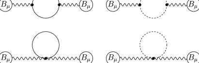
Figure 2: The Feynman diagrams that contribute to the effective action at $g^{2}$ order. Here the straight line and the dotted line represent the valence gluon and the ghost, respectively.

Now we repeat the perturbative calculation for QCD. We can do this either by calculating the one-loop Feynman diagrams directly, or by evaluating the integral (7) perturbatively to the order $g^{2}$. We start with the Feynman diagrams. For an arbitrary background $B_{\mu}$ there are four Feynman diagrams that contribute to the order $g^{2}$ which are shown in Fig. 2. Notice that the tadpole diagrams contain a quadratic divergence which does not appear in the final result.

The sum of these diagrams (in the Feynman gauge with dimensional regularization) gives us [15]

$$\Delta S=-\displaystyle\frac{11g^{2}}{96\pi^{2}}\int d^{4}pG_{\mu\nu}(p)G_{\mu\nu}(-p)\left[\mbox{ln}\left(\displaystyle\frac{p^{2}}{\mu^{2}}\right)+C_{1}\right],$$ (73)

where $C_{1}$ is a regularization-dependent constant. Clearly the imaginary part could only arise from the logarithmic term $\mbox{ln}(p^{2}/\mu^{2})$, so that for a space-like $p^{2}$ (with $\mu^{2}>0$) the effective action has no imaginary part. However, since a space-like $p^{2}$ corresponds to a magnetic background, we find that the magnetic condensation generates no imaginary part, at least at the order $g^{2}$. To evaluate the imaginary part for an electric background we have to make the analytic continuation of (73) to a time-like $p^{2}$, because the electric background corresponds to a time-like $p^{2}$. In this case the causality (again with the Feynman prescription $p^{2}\rightarrow p^{2}-i\epsilon$) dictates us to have

$$\mbox{ln}\Big{(}\displaystyle\frac{p^{2}}{\mu^{2}}\Big{)}\rightarrow\lim_{\epsilon\to 0}\mbox{ln}\Big{(}\displaystyle\frac{p^{2}-i\epsilon}{\mu^{2}}\Big{)}=\mbox{ln}\Big{(}\displaystyle\frac{|p^{2}|}{\mu^{2}}\Big{)}-i\displaystyle\frac{\pi}{2}~{}~{}~{}~{}~{}(p^{2}<0),$$ (74)

so that we obtain

$$Im~{}\Delta{\cal L}=\left\{{~{}~{}~{}~{}0~{}~{}~{}~{}~{}~{}~{}~{}~{}~{}~{}~{}(b=0),\atop-\displaystyle\frac{11b^{2}}{96\pi}~{}~{}~{}~{}~{}~{}~{}~{}~{}(a=0).}\right.$$

Obviously this is identical to (70). This allows us to conclude that the result (70) is indeed endorsed by the Feynman diagram calculation.

To remove any lingering doubt about (70) we now make the perturbative calculation of the integral (7) to the order $g^{2}$ with the Schwinger’s method, and find [13, 25]

$$\Delta S=-\displaystyle\frac{g^{2}}{8\pi^{2}}\int d^{4}pG_{\mu\nu}(p)G_{\mu\nu}(-p)\Sigma(p),$$

$$\Sigma(p)=\displaystyle\frac{}{}\int_{0}^{1}dv(1-\displaystyle\frac{v^{2}}{4})\displaystyle\frac{}{}\int_{0}^{\infty}\displaystyle\frac{dt}{t}\exp[-\displaystyle\frac{p^{2}}{4}(1-v^{2})t]$$

$$=2\displaystyle\frac{}{}\int_{0}^{1}dv\displaystyle\frac{v^{2}(1-v^{2}/12)}{1-v^{2}}+C_{2},$$ (75)

where $C_{2}$ is a regularization-dependent constants. Now, it is straightforward to evaluate the imaginary part of $\Delta S$. Comparing this with Schwinger’s result (71) for the massless QED we again reproduce (70), after the proper charge and wave function renormalization.

Furthermore, from the definition of the exponential integral function [16]

$$Ei(-z)=-\displaystyle\frac{}{}\int_{z}^{\infty}\displaystyle\frac{d\tau}{\tau}\exp(-\tau)=\gamma+\mbox{ln}z$$

$$+\displaystyle\frac{}{}\int_{0}^{z}\displaystyle\frac{d\tau}{\tau}\left[\exp(-\tau)-1\right]~{}~{}~{}({\rm Re}~{}z>0),$$ (76)

we can express $\Sigma(p)$ as

$$\Sigma(p)=-\displaystyle\frac{}{}\lim_{\epsilon\to 0}\int_{0}^{1}dv(1-\displaystyle\frac{v^{2}}{4})\left[\gamma+\mbox{ln}\Big{(}\displaystyle\frac{p^{2}}{4\mu^{2}}(1-v^{2})\epsilon\Big{)}\right]$$

$$=\displaystyle\frac{11}{12}\left[\mbox{ln}\left(\displaystyle\frac{p^{2}}{\mu^{2}}\right)+C_{3}\right],$$ (77)

where $C_{3}$ is another regularization-dependent constant. This tells that (75) is identical to (73). This is the reason why the perturbative calculation by Feynman diagrams and by Schwinger’s method produce the same result. This strongly indicates that the monopole condensation indeed describes a stable vacuum, but the electric background creates the pair-annihilation of the valence gluons in $SU(2)$ QCD [9, 13].

It might look surprising that both the infra-red regularization by causality and the perturbative method endorse the stability of the monopole condensation. But this is not accidental. In fact this is natural because both are based on the causality, which is what we need to exclude the unphysical tachyonic modes.

This confirms that the tachyonic modes are indeed unphysical mirage which should not have been there in the first place. They come into the calculation of the functional determinant by default. If so, one may ask how one can prevent this. Now we prove that a proper implementation of the gauge invariance excludes the tachyonic modes from the functional determinant.

7 Color Reflection Invariance: A Gauge Invariant Calculation of Functional Determinant

The effective action (7) is nothing but the vacuum to vacuum amplitude in the presence of the external field $\vec{B}_{\mu}$ [15],

$$\exp\Big{[}iS_{eff}(\vec{B}_{\mu})\Big{]}=<\Omega_{+}|~{}\Omega_{-}>\Big{|}_{\vec{B}_{\mu}}$$

$$=\displaystyle\frac{}{}\sum_{|n_{i}>}<\Omega_{+}|~{}n_{i}><n_{i}~{}|~{}\Omega_{-}>\Big{|}_{\vec{B}_{\mu}},$$ (78)

where $|\Omega>$ is the vacuum and $|n_{i}>$ is a complete set of orthonormal states of QCD. In the integral expression (7) the summation in terms of the complete set of states is expressed by the functional integration (at one-loop level). Now, to calculate this vacuum to vacuum amplitude one must use the physical vacuum and physical spectrum. And clearly the physical spectrum should not include the unphysical tachyons, unless one wants to assert that the physical spectrum of QCD must contain the tachyonic modes. This means that $|n_{i}>$ should not include the unphysical acausal states. This justifies the exclusion of the unphysical states in the calculation of the effective action. The question now is how one can do so.

There are two ways to exclude the unphysical modes, when one calculates the functional determinant or when one makes the infra-red regularization. We have already shown how to do this when we make the infra-red regularization [2, 3].

Now we are ready to show that a correct evaluation of the functional determinant (33) automatically excludes the tachyonic modes. In fact we will show that the gauge invariance forbids them to qualify as the physical eigenstates of the functional determinant (33). In the absence of the tachyonic modes, of course, we have no infra-red divergence, and thus no need of any infra-red regularization. This tells that it is not the $\zeta$-function regularization, but the incorrect evaluation of the functional determinant (33), which causes the instability of the SNO vacuum.

When one evaluates the functional determinant (33), one must start from a gauge invariant background. Otherwise the effective action will not remain gauge invariant. This means that the backgrounds (11) and (19) must be invariant under the background gauge transformation (2). But obviously the background (11) is not gauge invariant, so that one must impose the gauge invariance by hand in the calculation of the functional determinant (14). Of course, one could choose a particular gauge to calculate the determinant, but one should make sure that the gauge invariance is properly implemented in the calculation.

To discuss the gauge invariance it is important to understand the color reflection invariance in QCD [2, 3]. Consider the decomposition (20) again. As we have already noted, the decomposition (20) can be defined only up to the color reflection (26). This tells that the electric potential $A_{\mu}$ in (20), and thus the color charge in QCD, can uniquely be defined only up to this reflection degrees of freedom, even after one has chosen one’s color direction [2, 3]. Furthermore, this means that any physical state must be invariant under the the color reflection group generated by (26). To understand this in physical terms, consider a $q\bar{q}$ state. There are two color neutral states

$$|C,C_{3}>=|0,0>=\displaystyle\frac{|r\bar{r}>+~{}|b\bar{b}>}{\sqrt{2}},$$

$$|C,C_{3}>=|1,0>=\displaystyle\frac{|r\bar{b}>-~{}|b\bar{r}>}{\sqrt{2}},$$ (79)

where $r$ and $b$ represent the red and blue quark. But obviously only the first one is color singlet, and thus qualifies as a physical state. Now, notice that under the color reflection (26) the role of red and blue colors are interchanged, and only the color singlet state remains invariant under the color reflection. This shows that the color reflection invariance is an important symmetry, a prerequisite for a physical state, of QCD [2, 3]. In $SU(2)$ (26) generates a 4-element color reflection group, and in $SU(3)$ the color reflection group forms a 24-element symmetry group.

Now let us go back to the Savvidy background (11) again and show that the gauge invariance excludes the tachyonic modes from the physical eigenstates. To implement the gauge invariance to the Savvidy background, notice that $\vec{G}_{\mu\nu}$ in (11) must be gauge covariant. So one should be able to change $\vec{G}_{\mu\nu}$ to $-\vec{G}_{\mu\nu}$ by a gauge transformation by rotating ${\hat{n}}_{0}$ to $-{\hat{n}}_{0}$. In terms of $\bar{H}_{\mu\nu}$, this means that one can change $\bar{H}_{\mu\nu}$ to $-\bar{H}_{\mu\nu}$ by a gauge transformation. But obviously the gluon spin is not affected by this gauge transformation. This means that one can change the spin polarization direction of the gluon with respect to the magnetic field by a gauge transformation, which tells that the gauge invariant magnetic background can not have a polarization direction. Consequently the gauge invariant eigenvalues of the equation (12) must be those which are invariant under the transformation $H$ to $-H$. This, in turn, means that only the eigenstates which are invariant under the spin flip $(S_{3}\rightarrow-S_{3})$ of the valence gluon can be treated as the physical states. This is nothing but the color reflection invariance. Now, it must be clear that the tachyonic states (more precisely the eigenstates with $S_{3}=-1$ and $n=0$) are precisely the states which violate this color reflection invariance. This is shown schematically in Fig. 1, where (A) transforms to (B) under the color reflection. Notice that only the eigenstates with positive eigenvalues remain invariant under the color reflection. This tells that one must exclude the tachyonic states in one’s calculation of the effective action (14).

If one does so, the effective action (14) changes to

$$\Delta S=i\ln{\rm Det}\Big{[}(-\bar{D}^{2}+2gH)(-\bar{D}^{2}+2gH)\Big{]},$$ (80)

and we have

$$\Delta{\cal L}=\displaystyle\frac{}{}\lim_{\epsilon\rightarrow 0}\displaystyle\frac{1}{16\pi^{2}}\int_{0}^{\infty}\displaystyle\frac{dt}{t^{2-\epsilon}}\displaystyle\frac{gH/\mu^{2}}{\sinh(gHt/\mu^{2})}\Big{[}\exp(-2gHt/\mu^{2})+\exp(-2gHt/\mu^{2})\Big{]},$$ (81)

which has no infra-red divergence. This precludes the necessity to make any infra-red regularization.

The fact that $\bar{H}_{\mu\nu}$ does not change to $-\bar{H}_{\mu\nu}$ under the reflection $\hat{n}_{0}$ to $-\hat{n}_{0}$ in (11) simply confirms that the Savvidy background is not gauge invariant. This must be compared with the monopole background (19), which clearly has the advantage that it is invariant under the color reflection (26). Indeed not only $\vec{C}_{\mu}$ but also the background $\hat{A}_{\mu}$ itself is invariant under the color reflection (because the electric potential $A_{\mu}$ is uniquely defined only up to the signature).

Let us calculate the functional determinant (33) with this monopole background (19). Clearly we must honor the gauge invariance in the calculation. Unfortunately we did not. To see this consider ${\rm Det}(-{\hat{D}}^{2}+2iaN)(-{\hat{D}}^{2}-2iaN)$ in (33) first. This is made of two determinants,

$${\rm Det}(-{\hat{D}}^{2}+2iaN)={\rm Det}(-\tilde{D}^{2}+2a)^{2},$$

$${\rm Det}(-{\hat{D}}^{2}-2iaN)={\rm Det}(-\tilde{D}^{2}-2a)^{2},$$ (82)

and we have to solve the eigenvalue problem for each determinant separately. At first sight it appears that only the second determinant contains the tachyonic eigenstates. However, observe that ${\hat{D}}^{2}$ is invariant under (26), but $N_{ab}$ changes the signature. So the two determinants are the color reflection counterpart of each other. This means that, after the color reflection, it becomes the first determinant which contains the tachyonic eigenstates when $k^{2}<a$. From this it must become clear that actually both determinants contain the tachyonic eigenstates. More importantly, in both determinants, the tachyonic eigenstates are precisely those which do not remain invariant under the color reflection. Furthermore, the color reflection invariance tells that the two determinants must have identical eigenvalues. This means that the physical eigenstates of ${\rm Det}(-{\hat{D}}^{2}+2iaN)(-{\hat{D}}^{2}-2iaN)$ must be given by

$${\rm Det}(-\tilde{D}^{2}+2a)^{2}(-\tilde{D}^{2}+2a)^{2},$$ (83)

not by

$${\rm Det}(-\tilde{D}^{2}+2a)^{2}(-\tilde{D}^{2}-2a)^{2},$$ (84)

and should not contain any tachyonic states.

Exactly the same argument applies to ${\rm Det}(-{\hat{D}}^{2}+2bN)(-{\hat{D}}^{2}-2bN)$ in (33), made of two determinants

$${\rm Det}(-{\hat{D}}^{2}+2bN)={\rm Det}(-\tilde{D}^{2}-2ib)^{2},$$

$${\rm Det}(-{\hat{D}}^{2}-2bN)={\rm Det}(-\tilde{D}^{2}+2ib)^{2}.$$ (85)

In this case only the second determinant appears to have acausal eigenstates propagating backward in time when $k^{2}<b$, where $k$ is the momentum of eigenstate in the direction of the background color electric field. But again, the above argument tells that the two determinants are the color reflection counterpart of each other. So, under the color reflection the role of the first and second determinants are interchanged, and only the causal eigenstates which become invariant under the color reflection qualify as the physical eigenstates. From this we conclude that ${\rm Det}(-{\hat{D}}^{2}+2bN)(-{\hat{D}}^{2}-2bN)$ should be written as

$${\rm Det}(-\tilde{D}^{2}-2ib)^{2}(-\tilde{D}^{2}-2ib)^{2},$$ (86)

not as

$${\rm Det}(-\tilde{D}^{2}-2ib)^{2}(-\tilde{D}^{2}+2ib)^{2}.$$ (87)

So, excluding the unphysical eigenstates we have

$$\ln{\rm Det}K=\ln{\rm Det}\Big{[}(-{\hat{D}}^{2}+2iaN)(-{\hat{D}}^{2}+2iaN)\Big{]}_{ab}$$

$$+\ln{\rm Det}\Big{[}(-{\hat{D}}^{2}+2bN)(-{\hat{D}}^{2}+2bN)\Big{]}_{ab}$$

$$=2\ln{\rm Det}(-\tilde{D}^{2}+2a)(-\tilde{D}^{2}+2a)+2\ln{\rm Det}(-\tilde{D}^{2}-2ib)(-\tilde{D}^{2}-2ib).$$ (88)

From this we finally have

$$\Delta S=i\ln{\rm Det}[(-\tilde{D}^{2}+2a)(-\tilde{D}^{2}+2a)]+i\ln{\rm Det}[(-\tilde{D}^{2}-2ib)(-\tilde{D}^{2}-2ib)]$$

$$-2i\ln{\rm Det}(-\tilde{D}^{2}),$$ (89)

and

$$\Delta{\cal L}=\displaystyle\frac{}{}\lim_{\epsilon\rightarrow 0}\displaystyle\frac{1}{16\pi^{2}}\int_{0}^{\infty}\displaystyle\frac{dt}{t^{3-\epsilon}}\displaystyle\frac{abt^{2}/\mu^{4}}{\sinh(at/\mu^{2})\sin(bt/\mu^{2})}\Big{[}\exp(-2at/\mu^{2})+\exp(-2at/\mu^{2})$$

$$+\exp(+2ibt/\mu^{2})+\exp(+2ibt/\mu^{2})-2\Big{]}.$$ (90)

Obviously this has no infra-red divergence. This tells that, only when one mistakenly includes the unphysical eigenstates in the calculation of the functional determinant, one has to worry about which infra-red regularization is the correct one.

In retrospect we could have asserted that the tachyonic modes should be excluded from the functional determinant simply by saying that they are unphysical, because violate the causality. Clearly this is a correct assertion. But without an independent justification of this one might have objected this assertion. The above analysis tells that we can actually make this assertion, because we now have an independent verification of this assertion with the gauge invariance.

At this point we must clarify the meaning of the gauge invariant background. By this we do not mean that the background $\vec{G}_{\mu\nu}$ is gauge invariant. It must be gauge covariant. By a gauge invariant background we mean $\vec{G}_{\mu\nu}^{2}$ of a gauge covariant $\vec{G}_{\mu\nu}$. Exactly the same interpretation applies to the Lorentz invariance. In this sense our vacuum made of the monopole condensation is clearly gauge invariant as well as Lorentz invariant. Of course one could choose any gauge one likes to calculate the functional determinant (33). For example for the monopole background one can certainly choose a gauge where $\hat{n}$ becomes $\hat{n}_{0}$. When one does that the monopole background becomes $H_{\mu\nu}\hat{n}_{0}$, which looks almost identical to the Savvidy background $\bar{H}_{\mu\nu}\hat{n}_{0}$. But we emphasize that even in this gauge it remains invariant under the color reflection, because $H_{\mu\nu}$ transforms to $-H_{\mu\nu}$ under (26).

Now, one can integrate (90) and obtain [9, 13]

$${\cal L}_{eff}=\left\{\begin{array}[]{ll}-\displaystyle\frac{a^{2}}{2g^{2}}-\displaystyle\frac{11a^{2}}{48\pi^{2}}(\ln\displaystyle\frac{a}{\mu^{2}}-c),~{}~{}~{}~{}~{}b=0\\ ~{}\displaystyle\frac{b^{2}}{2g^{2}}+\displaystyle\frac{11b^{2}}{48\pi^{2}}(\ln\displaystyle\frac{b}{\mu^{2}}-c)\\ -i\displaystyle\frac{11b^{2}}{96\pi},~{}~{}~{}~{}~{}~{}~{}~{}~{}~{}~{}~{}~{}~{}~{}~{}~{}~{}~{}~{}~{}~{}~{}~{}~{}~{}~{}~{}a=0\end{array}\right.$$ (94)

which is identical to the effective action that we obtained with the infra-red regularization by causality. It is really remarkable that two completely independent principles, the gauge invariance and the causality, produce exactly the same effective action in QCD.

Observe that the effective action (94) with $a=0$ and $b=0$ are related by the electric-magnetic duality [9, 11]. In fact we can obtain one from the other simply by replacing $a$ with $-ib$ and $b$ with $ia$. This duality, which states that the effective action should be invariant under the replacement

$$a\rightarrow-ib,~{}~{}~{}~{}~{}~{}~{}b\rightarrow ia,$$ (95)

was first discovered in the effective action of QED recently [11, 12]. But subsequently this duality has also been shown to exist in the QCD effective action [9]. This tells that the electric-magnetic duality should be regarded as a fundamental symmetry of the effective action of gauge theory, both Abelian and non-Abelian. The importance of this duality is that it provides a very useful tool to check the self-consistency of the effective action. The fact that (67) and (69) are related by the duality assures that the infra-red regularization by causality is self-consistent.

The effective action (94) generates the much desired dimensional transmutation in QCD, the phenomenon Coleman and Weinberg first observed in massless scalar QED [5]. To demonstrate this we first renormalize the effective action. Notice that the effective action (94) provides the following effective potential

$$V=\displaystyle\frac{a^{2}}{2g^{2}}\Big{[}1+\displaystyle\frac{11g^{2}}{24\pi^{2}}(\ln\displaystyle\frac{a}{\mu^{2}}-c)\Big{]}.$$ (96)

So we define the running coupling $\bar{g}$ by [6, 9]

$$\frac{\partial^{2}V}{\partial a^{2}}\Big{|}_{a=\bar{\mu}^{2}}=\frac{1}{\bar{g}^{2}}.$$ (97)

With the definition we find

$$\frac{1}{\bar{g}^{2}}=\frac{1}{g^{2}}+\frac{11}{24\pi^{2}}(\ln\frac{{\bar{\mu}}^{2}}{\mu^{2}}-c+\displaystyle\frac{3}{2}),$$ (98)

from which we obtain the following $\beta$-function,

$$\beta(\bar{\mu})=\bar{\mu}\displaystyle\frac{\partial\bar{g}}{\partial\bar{\mu}}=-\frac{11\bar{g}^{3}}{24\pi^{2}}.$$ (99)

This is exactly the same $\beta$-function that one obtained from the perturbative QCD to prove the asymptotic freedom [27]. The fact that the $\beta$-function obtained from the effective action becomes identical to the one obtained by the perturbative calculation is remarkable, because this is not always the case. In fact in QED it has been shown that the running coupling and the $\beta$-function obtained from the effective action is different from those obtained from the perturbative method [11, 12].

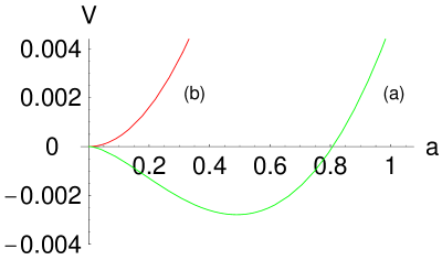
Figure 3: The effective potential of SU(2) QCD in the pure magnetic background. Here (a) is the effective potential and (b) is the classical potential.

In terms of the running coupling the renormalized potential is given by

$$V_{\rm ren}=\displaystyle\frac{a^{2}}{2\bar{g}^{2}}\Big{[}1+\displaystyle\frac{11\bar{g}^{2}}{24\pi^{2}}(\ln\displaystyle\frac{a}{\bar{\mu}^{2}}-\displaystyle\frac{3}{2})\Big{]},$$ (100)

which generates a non-trivial local minimum at

$$<a>=\bar{\mu}^{2}\exp\Big{(}-\frac{24\pi^{2}}{11\bar{g}^{2}}+1\Big{)}.$$ (101)

Notice that with ${\bar{\alpha}}_{s}=1$ we have

$$\displaystyle\frac{<a>}{{\bar{\mu}}^{2}}=0.48988....$$ (102)

This is nothing but the desired magnetic condensation. The corresponding effective potential is plotted in Fig. 3, where we have assumed $\bar{\alpha}_{s}=1$ and $~{}\bar{\mu}=1$.

Nelsen and Olesen have suggested that the existence of the unstable tachyonic modes are closely related with the asymptotic freedom in QCD [7]. Our analysis tells that this is not true. Obviously our asymptotic freedom follows from a stable monopole condensation.

8 Discussion

To eastablish the monopole condensation in QCD with the effective action has been extremely difficult to attain. The central issue here has been the stability of the monopole condensation. The earlier attempts to prove the monopole condensation have produced a negative result. The effective action of QCD in the presence of pure magnetic background calculated first by Savvidy and subsequently by Nielsen and Olesen did produce a non-trivial magnetic condensation [6, 7]. Unfortunately the SNO vacuum was unstable, due to the tachyonic modes in the functional determinant of the gluon loop. Nielsen and Olesen have correctly conjectured that the instability of the SNO vacuum originates from the fact that it is not gauge invariant. To cure this defect they have proposed the Copenhagen vacuum [7].

In this paper we have shown that there is much simpler and more natural way to implement the gauge invariance, to impose the color reflection invariance to the SNO vacuum. The color reflection invariance clearly shows that the tachyonic modes are the gauge artifact which are not gauge invariant. This disqualifies them as physical states. In the absence of the tachyons, of course, we have a stable monopole condensation and the dimensional transmutation in QCD. This endorses the conjecture of Nielsen and Olesen.

It is not surprising that the gauge invariance plays the crucial role in the stability of the monopole condensation. From the beginning the gauge invariance has been the main motivation for the confinement in QCD. It is this gauge invariance which forbids any colored object from the physical spectrum of QCD. This necessitates the confinement of color. So it is only natural that the gauge invariance assures the stability of the monopole condensation, and thus the confinement of color.

As we have pointed out, there are two ways to exclude the unphysical tachyonic states in the calculation of the effective action. One could either exclude them when one calculates the functional determinant (33), imposing the gauge invariance properly as we did in this paper. If one does this, the integral expression of the effective action (90) has no infra-red divergence and thus there is no need of any infra-red regularization. Or one could include them at this stage, and remove them later. If one chooses to do so, one obtains the integral expression (63) of effective action which has a severe infra-red divergence. In this case one must exclude them with the infra-red regularization by causality, not with the $\zeta$-function regularization [9, 13]. The reason is that the $\zeta$-function regularization does not remove any states included in the determinant. This does not mean that the $\zeta$-function regularization has any intrinsic deficiency. On the contrary the $\zeta$-function regularization is too honest to change the functional determinant (62).

Given the importance of the issue, however, one may need a further varification of the monopole condensation. One can do this with the perturbative calculation of the imaginary part of the one-loop effective action [10, 13]. This is made possible, because in QCD (and in massless QED) the imaginary part of the one-loop effective action is of the order $g^{2}$. This allows us to make a perturbative expansion of the imaginary part of the effective action. The perturbative calculation produces an identical result, identical to the the infra-red regularization by causality [13]. This again endorses the stability of the monopole condensation.

One might like to think that the existence of the tachyonic eigenstates is an essential characteristic, a sacred feature, of QCD. Indeed the tachyonic modes have been an enigma, the Gordian knot in QCD. It was there, and nobody knew how to resolve this puzzle. Nielsen and Olesen treated them as a sacred feature of QCD, which made it more mysterious. In this paper we have argued that the tachyons are an unphysical mirage which should not have been there in the first place. Actually it is not rare for us to encounter tachyonic states in physics, which appear when one does something improper or encounters something unphysical. Consider a spontaneously broken Abelian gauge theory coupled to a charged scalar field. In this case tachyons appear when one chooses a wrong vacuum, but they disappear when one chooses the correct one. Similarly, in bosonic string the vacuum state becomes tachyonic, but this problem disappears when we supersymmetrize the bosonic string. In QCD we have the same situation. Our analysis tells that the tachyonic eigenstates appear because we have not implemented the gauge invariance properly. With a proper implementation of the gauge invariance, they disappear. So there is nothing mysterious about the tachyons in QCD.

To summarize, we have presented three independent arguments which support the stability of the monopole condensation in QCD, the gauge invariance (the color reflection invariance) of the vacuum, the infra-red regularization of effective action by causality, and the perturbative calculation of the imaginary part of effective action, all of which endorse the stability of the monopole condensation. Furthermore all these calculations have been shown to be consistent with duality, a fundamental symmetry of effective action in gauge theories. This should be enough to settle the controversy on the stability of the monopole condensation in QCD once and for all. With this we can conclude that the quantum fluctuation does create a dimensional transmutation in QCD, triggered by the monopole condensation. This strongly implies that QCD is a theory of confinement in which all colored objects are confined by the dual Meissner effect.

In this paper we have considered only the pure magnetic or pure electric background. So, to be precise, the above result only proves the existence of a stable monopole condensation for a pure magnetic background. To show that this is the true vacuum of QCD, one must calculate the effective action with an arbitrary background in the presence of the quarks and show that the monopole condensation remains a true minimum of the effective potential. Fortunately, one can actually calculate the effective action with an arbitrary constant background, and show that indeed the monopole condensation becomes the true vacuum of $SU(2)$ QCD, at least at one-loop level [28]. Furthermoer, we have neglected the quarks in this paper. We simply remark that the quarks, just like in asymptotic freedom, tend to destabilize the monopole condensation. In fact the stability puts exactly the same constraint on the number of quarks as the asymptotic freedom [28].

It is truly remarkable (and surprising) that the principles of quantum field theory allow us to demonstrate confinement within the framework of QCD. There has been a proof of monopole condensation in a supersymmetric QCD [4]. Our analysis shows that one can actually establish the existence of the confinement phase within the conventional QCD, with the existing principles of quantum field theory. This should be interpreted as a most spectacular triumph of quantum field theory itself.

Acknowledgements

We thank Professor S. Adler and Professor F. Dyson for the fruitful discussions, and Professor C. N. Yang for the encouragements. This work is supported in part by the ABRL Program of Korea Science and Engineering Foundation (R14-2003-012-01002-0) and by BK21 Project of Ministry of Education.

References

-
[1]
Y. Nambu, Strings, monopoles and gauge fields,
Phys. Rev. D 10 (1974) 4262;
S. Mandelstam, Vortices and quark confinement in non-abelian gauge theories, Phys. Rept. 23 (1976) 245;
A.M. Polyakov, Quark confinement and topology of gauge groups, Nucl. Phys. B 120 (1977) 429;
G. ’t Hooft, Topology of the gauge condition and new confinement phases in nonabelian gauge theories, Nucl. Phys. B 190 (1981) 455. - [2] Y.M. Cho, A restricted gauge theory, Phys. Rev. D 21 (1980) 1080; A theory of monopoles, J. Korean Phys. Soc.17 (1984) 266; Abelian dominance in Wilson loops, Phys. Rev. D 62 (2000) 074009 [hep-th/9905127].
-
[3]
Y.M. Cho, Glueball spectrum in extended quantum chromodynamics,
Phys. Rev. Lett. 46 (1981) 302; Extended gauge theory and its mass
spectrum,
Phys. Rev. D 23 (1981) 2415;
W.S. Bae, Y.M. Cho and S.W. Kimm, QCD versus Skyrme-Faddeev theory, Phys. Rev. D 65 (2002) 025005 [hep-th/0105163]. - [4] N. Seiberg and E. Witten, Electric-magnetic duality, monopole condensation and confinement in supersymmetric Yang-Mills theory, Nucl. Phys. B 426 (1994) 19 [hep-th/9407087]; Monopoles, duality and chiral symmetry breaking in supersymmetric QCD, Nucl. Phys. B 431 (1994) 484 [hep-th/9408099].
- [5] S.R. Coleman and E. Weinberg, Radiative corrections as the origin of spontaneous symmetry breaking, Phys. Rev. D 7 (1973) 1888.
- [6] G.K. Savvidy, Infrared instability of the vacuum state of gauge theories and asymptotic freedom, Phys. Lett. B 71 (1977) 133.
-
[7]
N.K. Nielsen and P. Olesen, An unstable Yang-Mills field
mode,
Nucl. Phys. B 144 (1978) 376;
H.B. Nielsen and P. Olesen, A quantum liquid model for the QCD vacuum: gauge and rotational invariance of domained and quantized homogeneous color fields, Nucl. Phys. B 160 (1979) 380;
C. Rajiadakos, A stable symmetrized Savvidy vacuum, Phys. Lett. B 100 (1981) 471. -
[8]
A. Yildiz and P.H. Cox, Vacuum behavior in quantum
chromodynamics, Phys. Rev. D 21 (1980) 1095;
M. Claudson, A. Yildiz and P.H. Cox, Vacuum behavior in quantum chromodynamics, II, Phys. Rev. D 22 (1980) 2022;
S.L. Adler, Effective action approach to mean field nonabelian statics and a model for bag formation, Phys. Rev. D 23 (1981) 2905;
W. Dittrich and M. Reuter, Effective QCD lagrangian with zeta function regularization, Phys. Lett. B 128 (1983) 321;
M. Reuter and W. Dittrich, Symmetry restoration by a magnetic field at high temperature, Phys. Lett. B 144 (1984) 99;
C.A. Flory, A selfdual gauge field, its quantum fluctuations and interacting fermions, Phys. Rev. D 28 (1983) 1425;
S.K. Blau, M. Visser and A. Wipf, Analytical results for the effective action, Int. J. Mod. Phys. A 6 (1991) 5409;
M. Reuter, M.G. Schmidt and C. Schubert, Constant external fields in gauge theory and the spin 0, 1/2, 1 path integrals, Ann. Phys. (NY) 259 (1997) 313 -
[9]
Y.M. Cho, H.W. Lee and D.G. Pak, Faddeev-Niemi conjecture and
effective action of QCD, Phys. Lett. B 525 (2002) 347 [hep-th/0105198];
Y.M. Cho and D.G. Pak, Monopole condensation in QCD, Phys. Rev. D 65 (2002) 074027 [hep-th/0201179]. - [10] V. Schanbacher, Gluon propagator and effective lagrangian in QCD, Phys. Rev. D 26 (1982) 489.
-
[11]
Y.M. Cho and D.G. Pak, Effective action — a convergent series
— of QED, Phys. Rev. Lett. 86 (2001) 1947 [hep-th/0006057];
Y.M. Cho, Reply to comment on ‘Effective action: a convergent series of QED’, Phys. Rev. Lett. 91 (2003) 039101 [hep-th/0303040]. -
[12]
W.S. Bae, Y.M. Cho and D.G. Pak, Electric-magnetic duality in
QED effective action, Phys. Rev. D 64 (2001) 017303 [hep-th/0011196];
Y.M. Cho and D.G. Pak, Renormalization of QED effective action, [hep-th/0010073]. -
[13]
Y. M. Cho, M. L. Walker, and D. G. Pak, Monopole
condensation and dimensional transmutation in QCD,
J. High Energy Phys. 05 (2004) 073 [hep-th/0209208];
Y. M. Cho and M. L. Walker, Stability of Monopole Condensation in QCD, Mod. Phys. Lett. A 19 (2004) 2707 [hep-th/0206127]. - [14] B. de Witt, Quantum theory of gravity: the manifestly covariant theory, Phys. Rev. 162 (1967) 1195; Quantum theory of gravity: applications of the covariant theory, Phys. Rev. 162 (1967) 1239.
-
[15]
See for example, C. Itzykson and J. Zuber, Quantum field
theory, McGraw-Hill, New York 1980;
M. Peskin and D. Schröeder, An introduction to quantum field theory, Addison-Wesley, Reading 1995;
S. Weinberg, Quantum Theory of Fields, Cambridge University Press, Cambridge 1996. -
[16]
See, for example, I. Gradshteyn and I. Ryzhik,
Table of integrals, series and products, A. Jeffery ed.,
Academic Press, New York 1994;
M. Abramowitz and I. Stegun, Handbook of mathematical functions, Dover 1970. - [17] T.T. Wu and C.N. Yang, Concept of nonintegrable phase factors and global formulation of gauge fields, Phys. Rev. D 12 (1975) 3845.
- [18] Y.M. Cho, Colored monopoles, Phys. Rev. Lett. 44 (1980) 1115; Internal structure of the monopoles, Phys. Lett. B 115 (1982) 125.
-
[19]
A.A. Belavin, A.M. Polyakov, A.S. Shvarts and Y.S. Tyupkin,
Pseudoparticle solutions of the Yang-Mills equations,
Phys. Lett. B 59 (1975) 85;
G. ’t Hooft, Symmetry breaking through Bell-Jackiw anomalies, Phys. Rev. Lett. 37 (1976) 8. - [20] Y.M. Cho, Vacuum tunneling in spontaneously broken gauge theory, Phys. Lett. B 81 (1979) 25.
- [21] L.D. Faddeev and A.J. Niemi, Partially dual variables in Yang-Mills theory, Phys. Rev. Lett. 82 (1999) 1624 [hep-th/9807069]; Partial duality in Yang-Mills theory, Phys. Lett. B 449 (1999) 214 [hep-th/9812090].
-
[22]
S.V. Shabanov, An effective action for monopoles and knot
solitons in Yang-Mills theory, Phys. Lett. B 458 (1999) 322
[hep-th/9903223];
S.V. Shabanov, Yang-Mills theory as an abelian theory without gauge fixing, Phys. Lett. B 463 (1999) 263 [hep-th/9907182];
H. Gies, Wilsonian effective action for Yang-Mills theory with Cho-Faddeev-Niemi-Shabanov decomposition, Phys. Rev. D 63 (2001) 125023 [hep-th/0102026]. -
[23]
Y. M. Cho, Higher-dimensional unifications of gravitation
and gauge theories, J. Math. Phys. 16 (1975) 2029;
Y. M. Cho and P. S. Jang, Unified geometry of internal space with space-time, Phys. Rev. D 12 (1975) 3789. - [24] R. Zucchini, Global aspects of abelian and center projections in gauge theory, [hep-th/0306287].
- [25] A similar calculation was first carried out by Honerkamp. See J. Honerkamp, The question of invariant renormalizability of the massless Yang-Mills theory in a manifest covariant approach, Nucl. Phys. B 48 (1972) 269.
- [26] J. Schwinger, On gauge invariance and vacuum polarization, Phys. Rev. 82 (1951) 664.
-
[27]
D.J. Gross and F. Wilczek, Ultraviolet behavior of non-abelian
gauge theories, Phys. Rev. Lett. 30 (1973) 1343;
H.D. Politzer, Reliable perturbative results for strong interactions?, Phys. Rev. Lett. 30 (1973) 1346. - [28] Y.M. Cho and D.G. Pak, Dynamical symmetry breaking and magnetic confinement in QCD, [hep-th/0006051]; See also, Dynamical symmetry breaking and magnetic confinement in QCD in Proceedings of TMU-Yale Symposium on Dynamics of Gauge Fields, T. Appelquist and H. Minakata eds., Universal Academy Press, Tokyo 1999.