PUPT-2059

hep-th/0301002

Universality classes for horizon instabilities

Steven S. Gubser¹ and Arkadas Ozakin²

¹ Joseph Henry Laboratories, Princeton University, Princeton, NJ 08544 ² Lauritsen Laboratories of Physics, Caltech, Pasadena, CA 91125

Abstract

We introduce a notion of universality classes for the Gregory-Laflamme instability and determine, in the supergravity approximation, the stability of a variety of solutions, including the non-extremal D3-brane, M2-brane, and M5-brane. These three non-dilatonic branes cross over from instability to stability at a certain non-extremal mass. Numerical analysis suggests that the wavelength of the shortest unstable mode diverges as one approaches the cross-over point from above, with a simple critical exponent which is the same in all three cases.

December 2002

1 Introduction

The Gregory-Laflamme instability [1, 2] has been conjectured to arise precisely when local thermodynamic instabilities exist, for horizons with infinite extent and a translational symmetry [3, 4]. The idea is that, barring finite volume effects or some unexpected consequences of a curved horizon, the horizon will tend to become lumpy through real-time dynamics precisely if it can gain entropy by doing so. Based on this line of thinking, one might poetically ascribe the dynamical stability of the Schwarzschild black hole in four dimensions merely to the fact that the horizon is smaller in total size than the shortest wavelength instability.

A fairly thorough analysis in [5], exploiting a connection between time-independent, finite-wavelength perturbations in Lorentzian signature and negative modes in Euclidean signature, gives considerable confidence that the conjecture of [3, 4] is correct, as well as making clearer the reasons why thermodynamic and dynamical stability should be connected. The analysis of [5] does leave several points open, including the following:

1. For the black brane solutions familiar from string theory, just when is stability lost?

2. What happens near the threshold of stability?

3. Once an instability develops, what does the system evolve into?

Question 3) has been the subject of recent scrutiny for the case of uncharged black branes (see for instance [6, 7, 8, 9, 10]). Question 1) is straightforward if one grants the analysis of [5], since one needs only compute the specific heat as a function of non-extremality. We will address the question in section 2 from this thermodynamic point of view, and in section 4 by directly searching for time-independent, finite-wavelength perturbations, thus providing an independent check on the validity of the analysis of [5]. We will also make a start on question 2), based on our numerics. In section 3 we will introduce a notion of universality classes for black brane horizons, based on solutions described in [11]. For the questions we will address, a single characteristic exponent defines a universality class: this exponent describes how horizon entropy scales with temperature.

Our notion of universality classes is of some intuitive use in understanding the stability properties of various charged brane solutions. In particular, the well-known non-extremal D$p$-branes of type II string theory interpolate between one universality class far from extremality (where the entropy scales as a negative power of temperature, and Gregory-Laflamme instabilities exist) to a different universality class near extremality (where entropy scales as a positive power of temperature, and Gregory-Laflamme instabilities probably do not exist).

Other recent work on the Gregory-Laflamme instability includes [12, 13, 14]. In particular, [12] explores the stability of charged brane solutions, using methods somewhat different from ours, but with conclusions that overlap and agree with those in section 4.

2 Thermodynamic considerations

The D$p$-brane solutions to type II string theory have the following string frame metric and dilaton:

$${ds^{2}}$$

(1)

where

$${h=1-{r_{0}^{n}\over r^{n}}\qquad\qquad f=1+{r_{0}^{n}\sinh^{2}\alpha\over r^{n}}\,.}$$

(2)

The string metric $G_{\mu\nu}$ is related to the Einstein metric $g_{\mu\nu}$ by $g_{\mu\nu}=e^{-\phi/2}G_{\mu\nu}$. In equations (1) and (2), $n=7-p$. We will assume throughout that the metric (1) is being used to describe a large number $N_{p}$ of coincident D$p$-branes, so that the supergravity approximation is reliable (except perhaps near the horizon at extremality, where some of the solutions have a null singularity).

The thermodynamic properties of D$p$-branes are well-known, so we will present here only a brief summary. The original literature, including [15, 16, 17], can be consulted for further details. The entropy of the D$p$-brane solution (1) is

$${S={A_{\rm Einstein}\over 4G_{N}}={A_{\rm string}\over 4G_{N}e^{2\phi}}={4\pi\Omega_{n+1}\over 2\kappa^{2}}Vr_{0}^{n+1}\cosh\alpha\,,}$$

(3)

where $A_{\rm Einstein}$ is the horizon area measured using the Einstein frame metric, $A_{\rm string}$ is the horizon area in the string frame metric, $V$ is the coordinate volume in the $y^{i}$ directions, and $\Omega_{n+1}$ is the volume of the sphere $S^{n+1}$:

$${\Omega_{m}=\mathop{\rm Vol}\nolimits S^{m}=2{\pi^{m+1\over 2}\over\Gamma\left({m+1\over 2}\right)}\,.}$$

(4)

If one compactified the $y^{i}$ on a torus whose volume at infinity was $V$, then (3) would be the total entropy of the resulting horizon. The ADM mass (most easily calculated using the Einstein frame metric) is

$${M={\Omega_{n+1}V\over 2\kappa^{2}}r_{0}^{n}\left({n+2\over 2}+{n\over 2}\cosh 2\alpha\right)\,.}$$

(5)

The temperature can be extracted from the surface gravity:

$${T={\kappa\over 2\pi}={1\over 2\pi}\left.{\partial g_{tt}/\partial r\over 2\sqrt{g_{tt}g_{rr}}}\right|_{r=r_{0}}={n\over 4\pi r_{0}\cosh\alpha}\,.}$$

(6)

One can substitute $G_{tt}$ and $G_{rr}$ for $g_{tt}$ and $g_{rr}$ in (6), provided the dilaton is non-singular at the horizon (which would just mean that the horizon is a null singularity, and that only happens for extremal D$p$-branes).

It is straightforward to check that $T=\partial M/\partial S$.

The D$p$-brane charge is quantized, and can be expressed in terms of the following constraint:

$${\tilde{R}^{n}\equiv{\textstyle{1\over 2}}r_{0}^{n}\sinh 2\alpha={2\kappa^{2}\over n\Omega_{n+1}}N_{p}\tau_{p}={N_{p}\sqrt{2\kappa^{2}(2\pi)^{7-2p}(\alpha^{\prime})^{3-p}}\over n\Omega_{n+1}}={(2\pi)^{n}\over n\Omega_{n+1}}\sqrt{\alpha^{\prime}}^{n}gN_{p}\,,}$$

(7)

where $N_{p}$ is an integer and $\tau_{p}$ is the tension of a single extremal D$p$-brane, and we have used the relation

$${16\pi G_{N}=2\kappa^{2}=(2\pi)^{7}g^{2}(\alpha^{\prime})^{4}\,,}$$

(8)

valid in uncompactified type II string theory. The formula (7), taken from [16], can be checked against the standard formula for D-brane tension:

$${2\kappa^{2}\tau_{p}^{2}=(2\pi)^{7-2p}(\alpha^{\prime})^{3-p}\,.}$$

(9)

Holding $N_{p}$ fixed, the behavior of the temperature in different limits is well known. In all cases, $T\to 0$ in the small $\alpha$ limit, since this is the large mass limit where the charge is negligible. For $p=1,2,3$, and $4$, $T\to 0$ also in the extremal limit, whereas for $p=5$, $T$ approaches a constant, and for $p=6$, $T$ diverges. There are no other remarkable qualitative features of the dependence of $T$ on mass other than a consequence of what we have already said: for $p<5$, there is a special mass $M_{*}$ where $T$ reaches a global maximum. This is the border of thermodynamic stability: for masses less than $M_{*}$, the specific heat is positive, and for masses greater than $M_{*}$ it is negative. Holding $N_{p}$ fixed, one finds that (6) is extremized when

$${\sinh^{2}\alpha=\sinh^{2}\alpha_{*}={1\over n-2}\,,}$$

(10)

or alternatively when

$${{M\over N_{p}\tau_{p}V}={M_{*}\over N_{p}\tau_{p}V}={n^{2}-2\over n\sqrt{n-1}}}$$

(11)

(note that $N_{p}\tau_{p}V$ is the extremal mass). Another characterization of the same condition is

$${r_{0}=r_{0}^{*}=\left({n-2\over\sqrt{n-1}}\right)^{1/n}\tilde{R}\,,}$$

(12)

where $\tilde{R}$ is the length scale introduced in (7).

The M2 and M5-brane metrics are given by

$${ds_{M2}^{2}}$$

(13)

where $f$ and $h$ are given by (2) with $n=6$ for the M2-brane and $n=3$ for the M5-brane. Indeed, the thermodynamics for the M2-brane and the D1-brane are identical. This is not accidental: wrapping an M2-brane around a circle gives a fundamental string of type IIA, which is equivalent through some further dualities to the D1-brane (and, more to the point, has the same Einstein metric up to a slightly different identification of parameters). For similar reasons, the M5-brane and D4-brane have the same thermodynamics. In particular, the condition for the maximum Hawking temperatures for the M2-brane and the M5-brane are given precisely by (10), (11), and (12), with $n=6$ and $3$, respectively.

3 Universality classes and the general problem

A fairly broad statement of the question of $p$-brane stability in the supergravity approximation can be summed up as follows: starting with some $p$-brane solution in supergravity, one wishes to consider perturbations that break some part of the translational invariance and determine whether any of them grow with time. Such considerations can often be reduced to a problem in $2+1$ dimensions, and in the following paragraphs we shall give more particulars about how this comes about.

One starts with a two-derivative action in $\hat{D}>2$ spacetime dimensions, containing Einstein gravity and perhaps also form fields and scalars. The brane in question is some solution with a horizon and a weakly curved region far from it (typically asymptotically flat space), where the whole solution admits as symmetries the Euclidean group of translations and rotations in $p$ dimensions. There should also be some Killing vector which is timelike in the weakly curved region and null at the horizon, which can be used to construct a notion of energy; and there may be assorted spacelike Killing vectors as well, indicating rotational symmetries. The brane is of spatial co-dimension $\hat{D}-1-p$, and far from the brane one generally expects an approximate $SO(\hat{D}-1-p)$ rotational symmetry group. The brane may have various conserved charges and angular momenta (the latter corresponding to generators of $SO(\hat{D}-1-p)$). In this rather general context, we would like to ascertain the stability properties of the solution against small perturbations (determined by thermodynamic stability, according to [3, 4, 5]), perhaps also the dispersion relation for such perturbations, and finally the end state of evolution along an unstable direction—though this last is surely a much harder problem in general than the other two.

Although we believe that the notion of universality classes we introduce below will have some applicability to the general case (including for example smeared brane solutions), let us focus on the case where the $SO(\hat{D}-1-p)$ symmetry is exact. Then perturbations can be labeled uniquely by their wave-number $\vec{k}$ along the brane and their angular momentum quantum numbers under $SO(\hat{D}-1-p)$. It seems reasonable to assume that the $s$-wave perturbations become unstable first, provided they exist as dynamical perturbations (as opposed to being perturbations which are pure gauge). The perturbations in question thus preserve a large subgroup of the symmetry of the original solution: $SO(\hat{D}-1-p)$ times that part of the Euclidean group that preserves $\vec{k}$. This makes it particularly natural to consider a Kaluza-Klein “reduction” where one integrates the action over an $S^{\hat{D}-2-p}$ orbit of $SO(\hat{D}-1-p)$, and drops the integration over an ${\bf R}^{p-1}$ perpendicular to $\vec{k}$. The result is a 2+1-dimensional action, which in a fairly broad set of circumstances can be brought into the form

$${S=\int d^{3}x\,\sqrt{g}\left(R-{1\over 2}G_{ij}(\vec{\phi})\partial_{\mu}\phi^{i}\partial^{\mu}\phi^{j}-V(\vec{\phi})\right)\,.}$$

(14)

Einstein gravity, form fields, and scalars in $\hat{D}$ dimensions reduce down to the type of action written in (14), plus perhaps abelian and non-abelian gauge fields. The abelian gauge fields can be dualized to scalars, unless there are Chern-Simons terms in the action. Non-abelian gauge fields in general cannot be dualized, but examples in the literature often have fields excited corresponding to an abelian subgroup. Thus (14), while obviously not completely general, does cover a broad range of cases. Furthermore, it has been observed [18] that $V(\vec{\phi})$ is commonly a sum of exponentials of canonically normalized scalars: for example, the integrated curvature of $S^{\hat{D}-2-p}$ scales as a power of its radius, but the canonically normalized scalar measuring the size of $S^{\hat{D}-2-p}$ is some multiple of the logarithm of the radius.

In section 3.1 we will consider properties of solutions to (14), in part recapitulating arguments of [18]. In section 3.2 we briefly remark on the reason to search for static perturbations. Then in section 3.3 we will make an explicit numerical study of stability of a special case of the solutions considered in section 3.1.

3.1 Solutions to gravity plus scalars

Let us now study the slightly more general situation where

$${S=\int d^{D}x\,\sqrt{g}\left(R-{1\over 2}G_{ij}(\vec{\phi})\partial_{\mu}\phi^{i}\partial^{\mu}\phi^{j}-V(\vec{\phi})\right)\,,}$$

(15)

where $D=d+1$ is unrelated to $\hat{D}$. Motivated by the previous discussion, we will be most interested in the case $D=3$. Solutions to the equations of motion of this action were studied in [18], of the form

$${ds^{2}=a(r)^{2}(-dt^{2}+d\vec{x}^{2})+dr^{2}\,,\qquad\vec{\phi}=\vec{\phi}(r)\,,}$$

(16)

with $a(r)$ a monotonically increasing function of $r$, running from $0$ to $\infty$. The large $a$ region in these solutions is weakly curved (in fact, the main interest in [18] was asymptotically anti-de Sitter space), and the small $a$ region is in most cases singular. These solutions have no horizons (or at best degenerate or singular horizons), and their symmetry under boosts amounts to the statement that they are extremal. All such solutions can be derived using a first order formalism (see for example [19, 20, 21]), which is a direct analog of the Hamilton-Jacobi method of generating FRW cosmologies [22]: if one starts with an action of the same form as (14), but in $D$ dimensions, and finds $W(\vec{\phi})$ such that

$${V(\phi)={1\over 2}G^{ij}{\partial W\over\partial\phi^{i}}{\partial W\over\partial\phi^{j}}-{1\over 4}{D-1\over D-2}W^{2}\,,}$$

(17)

then a solution to

$${{\partial\phi^{i}\over\partial r}=-G^{ij}{\partial W\over\partial\phi^{j}}\,,\qquad{\partial a/\partial r\over a}={1\over 2(D-2)}W(\vec{\phi})}$$

(18)

will also solve the equations of motion.

Non-extremal generalizations of (16) have the form

$${ds^{2}=a(r)^{2}(-h(r)dt^{2}+d\vec{x}^{2})+{dr^{2}\over h(r)}\,,\qquad\vec{\phi}=\vec{\phi}(r)\,.}$$

(19)

We assume in general that $h(r)\to 1$ in the region where $a(r)\to\infty$, and $h(r)<1$ everywhere. If $h(r_{H})=0$ and $r_{H}$ is the largest value of $r$ for which this is true, then $r=r_{H}$ is an event horizon with respect to the region where $a(r)\to\infty$ (which is also at large $r$). Provided $h^{\prime}(r_{H})\neq 0$, this is a non-degenerate horizon with finite Hawking temperature.

Solutions of the form (19) involve a number of constants of integration. The counting of them has been explained in [18], and we will recapitulate briefly here. The relevant equations of motion are all ordinary differential equations in $r$ once we assume the form (19). They comprise the second order equations for the scalars, of which we suppose there are $n$; the $G_{rr}$ component of Einstein’s equation, which is a first order equation; and one further Einstein equation (for instance, the combination $G^{t}{}_{t}-G^{x}{}_{x}$ of Einstein’s equations), which is second order. There are $2n+3$ integration constants altogether. One amounts to an additive shift in the radial variable $r$, which is just a coordinate transformation. Another is fixed by the requirement that $h(r)\to 1$ in the region where $a(r)$ is large. The presence of a non-degenerate horizon fixes $n$ more, as explained in [18] (one way to understand the presence of these $n$ horizon constraints is that in the Wick-rotated Euclidean solution, where the horizon becomes a point, the scalars must be smooth everywhere, so their radial derivatives must vanish at this point). This leaves $n+1$ parameters that specify the solution. One of these is the temperature of the horizon, and the other $n$ pertain to the asymptotics of the scalars in the large $a$ region. Of these $n$ parameters, some but not all may be fixed by demanding regularity in the large $a$ region. In an $AdS_{d+1}/CFT_{d}$ context, where the large $a$ region is asymptotically anti de-Sitter, the $n$ parameters correspond to the coefficients of $e^{-(d-\Delta_{i})r/L}$ in the expansion of the scalars around their constant limiting values as $r\to\infty$. These coefficients amount on the CFT side to the mass parameters of gauge singlet operators added to the lagrangian. If some of the operators in question are irrelevant, then the corresponding scalars have positive $m^{2}$, and the larger of the two solutions to the linearized scalar equations of motion blows up at large $r$: this is a case where parameters are fixed to zero by demanding regularity in the large $a$ region. In the case where the dual operators are relevant, and the corresponding scalars have negative $m^{2}$, then the coefficient of $e^{-(d-\Delta_{i})r/L}$ is truly a variable parameter. In the case of asymptotically anti-de Sitter solutions, an additional scaling symmetry can be used to eliminate one additional parameter: this amounts to applying a scale transformation on the CFT side to set, say, the temperature equal to $1$.

Let us now consider the situation where the asymptotics of the scalars is entirely fixed in the large $a$ region, leaving us with one free parameter. One can show (see [18] for the case where $d=4$) that

$${h=1-B\int_{r}^{\infty}{dr_{1}\over a(r_{1})^{d}}\,,}$$

(20)

and then $B$ is the free parameter. (The identity (20) holds even though $a(r)$ may in general change when $B$ changes. It is a convenient parametrization because the influence of $B$ on $a(r)$ is small in the large $a$ region). In an $AdS_{d+1}/CFT_{d}$ context, this would correspond to specifying a deformation of the gauge theory lagrangian by relevant operators and then varying either the temperature or the energy density. Evidently, in the limit $B\to 0$, one recovers a solution of the form (16). Suppose that in this limiting solution, $V(\vec{\phi}(r))$ decreases monotonically as $a(r)$ decreases, going to $\infty$ as $a\to 0$. It can then be argued (though not wholly rigorously) [18] that

• Solutions with regular horizons exist for all $B>0$.

• If $V(\vec{\phi})$ is the sum of exponentials of canonically normalized scalars, then in the $B=0$ solution, the scalars have an asymptotic direction as $a(r)\to 0$: that is, $\vec{\phi}(r)\sim\vec{\phi}_{0}+\vec{v}\varphi(r)$ for some constants $\vec{\phi}_{0}$ and $\vec{v}$, which we may normalize so that $\varphi$ is itself canonically normalized. Then $V(\vec{\phi}(r))\approx e^{2\gamma\varphi}$ in the region of small $a$.

• In near-extremal solutions, with sufficiently small $B$, the solution at small $a$ is well-approximated by a Chamblin-Reall solution for the exponent $\gamma$, which we explain below in section 3.3. The whole solution can be well-approximated by the original extremal solution patched onto a Chamblin-Reall solution. These approximations become progressively better as $B\to 0$.

• The entropy and temperature of near-extremal solutions are related by a power law: $S\propto VT^{\alpha}$, where

  $${\alpha={D-2\over 1-2\gamma^{2}(D-2)}\,.}$$

  (21)

These features suggest the notion of universality class that we are going to use. Suppose that an extremal solution to an action with canonically normalized scalars has a “scaling region” where $\vec{\phi}(r)\approx\vec{\phi}_{0}+\vec{v}\varphi(r)$ and $V\approx e^{2\gamma\varphi}$ for many decades of variation of $a(r)$. Then non-extremal solutions with the horizon well within the scaling region should again be well-approximated by the original extremal solution patched onto a Chamblin-Reall solution near the horizon. The approximation should become good in the limit where the scaling region in the extremal solution extends far above and below the value of $a$ where the horizon is located in the non-extremal solution. The same power law, $S\propto VT^{\alpha}$, should pertain.

With the idea of universality classes in hand, we can address stability of the horizon in a simple way. In section 3.3, we will study explicitly perturbations around Chamblin-Reall solutions, involving the metric and the “active” scalar $\varphi$. We will find perturbations which are normalizable both at the horizon and far from it. As the full solution is well approximated by matching the extremal solution onto a Chamblin-Reall solution, perturbations should be well approximated by similarly matched solutions—only, because the perturbations we are considering are normalizable within the Chamblin-Reall region, they approach zero near the matching region, and the perturbations of fields in the extremal region are very small. It does not seem plausible that there are normalizable perturbations which are large in the extremal region and small as one enters the Chamblin-Reall region near the horizon. To sum up, we believe the stability properties of the whole solution are determined by the stability properties of the near-horizon Chamblin-Reall solution, which also determines the scaling of entropy with temperature.

It may seem that we are focusing rather narrowly on a rather special class of perturbations: not only invariant under the $SO(\hat{D}-1-p)$ that we started with in carrying out the Kaluza-Klein reduction, but also involving only the metric and the active scalar near the horizon. This amounts to focusing on a type of fluctuations which we might describe as adiabatic, since the fields are varying locally in the same proportions that they would do globally if we simply changed the temperature. But this is precisely the mode of instability that the thermodynamic arguments of [3, 4, 5] suggest. Instabilities in other modes are conceivable, and one could even study them by considering scalar fluctuations “transverse” to the solution. But we would find it very surprising if such fluctuations gave rise to normalizable instabilities when the fluctuations we consider do not. To put it another way, for that to happen, the logic of [5] must fail. Our rather detailed predications about the nature of the instability amount in a sense to an elaboration of the connection between thermodynamic and dynamical instabilities.

3.2 Static perturbations

In the rest of this paper, we will investigate Gregory-Laflamme type instabilities of various black branes. For all the unstable black branes Gregory and Laflamme analyzed [1, 2], they found at linear order in perturbation theory that there is a static perturbation, and that instabilities occur at longer wavelengths than this static perturbation.

As remarked in the introduction, Reall [5] in his approach to the proof of the conjecture of [3, 4] investigated the role of such time-independent perturbations, and argued that they are of central importance to the relation between thermodynamic and dynamical instability. In particular he related such perturbations of a black-brane solution to the negative modes of the Lichnerowicz operator on the Euclidean black hole background found by compactifying the black $p$-brane on a $p$-torus and doing a Wick rotation. The existence of such negative modes is then related to thermodynamic stability. (Negative modes of Euclidean black holes have also been analyzed in the context of finite temperature stability of flat spacetime by Gross, Perry and Yaffe [23].)

Thus when looking for instabilities of black branes, instead of considering instabilities with arbitrary growth rates, we will restrict our attention to static threshold perturbations. With the relation between thermodynamic and dynamical stabilities in mind, we expect the dispersion curve of a Gregory-Laflamme type instability to end at such a threshold point at the small wavelength limit.

3.3 The Chamblin-Reall solutions

As argued in section 3.1, close to the horizon, black brane solutions [11] for gravity coupled to a scalar $\phi$ with a potential of the form $V=V_{0}e^{2\gamma\phi}$ provide good approximations to a broad range of supergravity solutions, including ones that are non-extremal versions of those that represent RG-flows in AdS/CFT.

The action for the gravity plus scalar system is

$${S}$$

(22)

We will restrict our attention to negative $V_{0}$, since that is the case that admits black hole solutions. The black brane solutions are given by

$${ds_{0}^{2}=a_{0}^{2}(r)(-h_{0}(r)dt^{2}+d\vec{x}_{D-2}^{2})+{dr^{2}\over h_{0}(r)}\,,}$$

(23)

where

$${h_{0}(r)}$$

(24)

and $c$ is given by the positive root of the equation

$${V_{0}=c^{2}\left({1\over 2}\gamma^{2}-{1\over 4}{D-1\over D-2}\right)\,.}$$

(25)

In the notation of [11] (differing slightly from ours), these solutions correspond to the “type II” case, with $b^{2}<D-1$, $M>0$, and $V_{0}<0$. Note that in the gauge presented above, the metric is independent of $V_{0}$: it only depends on $\gamma$, whereas the scalar profile depends on both $\gamma$ and $V_{0}$.

With respect to the general discussion of non-extremal horizons in section 3.1, the solution (24) is rather special, in that the functions $a(r)$ and $\phi(r)$ are entirely independent of the parameter $r_{0}$ that determines the location of the horizon. (The equivalent parameter in section 3.1 is $B$). In other words, one can get at the solution (24) by first obtaining the extremal solution and then using (20) without changing $a(r)$. In general, $h\neq 1$ “back-reacts” on the solution, changing $a(r)$ and $\phi(r)$. This property of (24) also hints at the origin of the relation (25): One plugs $W=ce^{\gamma\phi}$ in (17) to obtain $V$, just as one would do when looking for extremal solutions.

As noted in [11], for a discrete set of $\gamma$’s it is possible to arrive at the solutions (24), (25) by a dimensional reduction of spacetimes of the form $Schwarzchild_{q+2}\times R^{D-2}$ on the $q$-sphere of $Schwarzchild_{q+2}$. For such cases, $V_{0}$ and $\gamma$ are given in terms of $q$ as

$${V_{0}}$$

(26)

At least for this discrete set of solutions, we certainly expect to find dynamical instabilities: they correspond to the instabilities of an uncharged black string in $q+3$ spacetime dimensions. The $\gamma$’s that can be obtained by a dimensional reduction on a $q$-sphere, where $q$ runs from $1$ to $\infty$, fall in the range

$${\sqrt{1\over 2(D-2)}<\gamma<\sqrt{D-1\over 2(D-2)}\,.}$$

(27)

(The case $q=1$, which gives the upper limit on $\gamma$, is degenerate: $V_{0}=0$ for that case.) It turns out that (27) is precisely the range for which the $D$-dimensional black brane has a negative specific heat. The conjecture of [3, 4] then implies that one should have dynamical instabilities for the $\gamma$’s precisely in this range, including the ones that can’t be obtained by dimensional reduction. In the next section, we will give numerical evidence in favor of this for the case $D=3$. (The same conclusion for other $D$ then follows from straightforward Kaluza-Klein reduction).

3.4 Numerical study of the stability of Chamblin-Reall solutions

Choosing $D=3$, we searched numerically for threshold dynamical instabilities of the Chamblin-Reall solutions by restricting attention to perturbations of the form

$${ds^{2}}$$

(28)

where

$${A(r,x)}$$

(29)

and working to linear order in $\lambda$. It is possible to show that this ansatz for the perturbations is consistent with the equations of motion.

The Einstein equations in $D=3$ read

$${R^{\mu}_{\nu}=T^{\mu}_{\nu}-g^{\mu}_{\nu}T^{\alpha}_{\alpha}\,.}$$

(30)

Four of these equations are nontrivial, namely the ones involving $R^{t}_{t}$, $R^{r}_{r}$, $R^{x}_{x}$ and $R^{r}_{x}$. Using the $R^{r}_{x}$ equation, one can solve algebraically for $B_{1}$ in terms of $A_{1}$, $A_{1}^{\prime}$, and $\phi_{1}$. The $R^{t}_{t}$ equation and the scalar equation of motion involve $B_{1}$, but not its derivatives. Plugging in $B_{1}$ as found from the $R^{r}_{x}$ equation into the $R^{t}_{t}$ equation and the scalar equation of motion, we end up with the following two equations involving $A_{1}$ and $\phi_{1}$:

$${0}$$

(31)

(It is possible to do a consistency check by arriving at the same equations using the $R^{x}_{x}$ and $R^{r}_{r}$ equations).

We used the linearity of the equations to fix the value of $\phi_{1}$ at the horizon. Then, using a a shooting algorithm, we looked for values of $k$ and $A_{1}(r_{0})$ that would give solutions that are well-behaved at the horizon and infinity, for a given $\gamma$. The results for $k$ as a function of $\gamma$ are shown in figure 1. As can be seen from the figure, the wavelengths of the threshold instabilities diverge as one approaches the thermodynamic stability limit given by $\gamma=\gamma^{*}\equiv{1\over\sqrt{2}}$ (the lower limit in (27)). $\gamma=1$, which corresponds to the upper limit in (27), is where the causal structure of the Chamblin-Reall solutions changes: in the notation of Chamblin and Reall [11], going from $\gamma<1$ to $\gamma>1$ corresponds to going from the $b^{2}<D-1$ case to the $b^{2}>D-1$ case of the type II solutions.

For $\gamma<1/\sqrt{2}$, we found no static perturbation. This plus the thermodynamic stability of the solutions strongly suggests that they are stable.

In order to address the question of what happens near the threshold of instability, we attempted to fit the behavior of $k$ as a function of $\gamma$ to a power law near $\gamma=\gamma^{*}$. The fit was considerably better if the threshold of stability was shifted to $\gamma^{*}_{num}\approx 1.003\gamma^{*}$: then we found $k\sim\sqrt{\gamma-\gamma^{*}_{num}}$. The fit to a power law was still less than spectacular. We suspect that numerical error contributed both to this and to the discrepancy between $\gamma^{*}$ and $\gamma^{*}_{num}$.

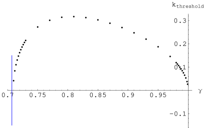
Figure 1: Stability of Chamblin-Reall solutions. The dots represent threshold instabilities of the Chamblin-Reall solutions. The vertical line at $\gamma^{*}=1/\sqrt{2}$ indicates the thermodynamic stability limit.

4 Crossing the threshold of stability: non-dilatonic
branes

Next, we would like to investigate the dynamical stability of D3, M2 and M5-branes. Following the philosophy introduced in the beginning of section 3, we will do a Kaluza-Klein reduction of the metrics (1) and (13) on all but one of the spatial worldvolume directions and $S^{n+1}$, to end up with a 3 dimensional background. We will be working with $s$-wave perturbations of this background, keeping only the two scalars that describe the sizes of $S^{n+1}$ and the torus, ignoring all the higher harmonics. There will be two contributions to the potential of these scalars: one due to the curvature of the $S^{n+1}$ that we compactify on, another due to the kinetic term of the 4-form (3-form) potential in IIB (eleven-dimensional) supergravity. Both of these terms will turn out to be exponentials of a linear combination of the two scalars, hence the notion of universality classes introduced in section 3 will be relevant in this context.

4.1 Kaluza-Klein reduction

We want to perform the dimensional reduction in a way that would give an Einstein-Hilbert action for gravity, without a scalar-dependent coefficient in front of the three-dimensional Ricci scalar. For this purpose, let’s start with a general metric

$${ds_{D}^{2}=d\bar{s}_{r}^{2}+e^{2K}ds_{p}^{2}+e^{2L}ds_{q}^{2}}$$

(32)

where $D=p+q+r$, $d\bar{s}_{r}^{2}$ is a metric on the Lorentzian $r$-manifold $X_{r}$, $ds_{p}^{2}$ and $ds_{q}^{2}$ are metrics on compact Riemannian manifolds $Y_{p}$ and $Z_{q}$, respectively, and $K$ and $L$ are functions that depend only on the coordinates of $X_{r}$. For example, for the case of the D3-brane, $p=2$, $Y_{p}=T^{2}$ (two worldvolume directions are compactified), $q=5$, $Z_{q}=S^{5}$, $r=3$. Defining

$${d\bar{s}_{r}^{2}=e^{2N}ds_{r}^{2}\,,}$$

(33)

with

$${N=-{pK+qL\over r-2}\,,}$$

(34)

one gets

$${\sqrt{-g_{D}}}$$

(35)

where $R(ds^{2})$ denotes the Ricci scalar for the metric $ds^{2}$. The first term gives the Einstein-Hilbert lagrangian for $ds_{r}^{2}$ (without a scalar-dependent factor—as we wanted), and the rest are the kinetic and potential terms for the scalars $K$ and $L$. In our applications, $R(ds_{p}^{2})$ and $R(ds_{q}^{2})$ will be the Ricci scalars of $T^{p}$ and $S^{q}$, respectively, i.e. 0 and $q(q-1)$.

Using these results, we get the dimensionally reduced form of the D3-brane metric and the scalars as

$${ds_{0}^{2}}$$

(36)

where $f$ and $h$ are given by (2) with $n=4$. The three-dimensional action is given by

$${S=\int d^{3}x\sqrt{g_{3}}\left(R-{1\over 2}\partial_{\mu}\phi^{i}\partial_{\nu}\phi^{j}G_{ij}g_{3}^{\mu\nu}-V(\vec{\phi})\right)}$$

(37)

where

$${G_{ij}=\left(\begin{array}[]{cc}12&20\\ 20&60\end{array}\right)\qquad\qquad\vec{\phi}=\left(\begin{array}[]{c}K\\ L\end{array}\right)}$$

(38)

$${V(\vec{\phi})=-20e^{-4K-12L}+8\tilde{R}_{D3}^{8}e^{-4K-20L}\,,}$$

(39)

and $\tilde{R}_{D3}$ is the length scale defined in (7), with $n=4$. The first term in $V$ comes from (35), and the second one comes from the dimensional reduction of the $F_{5}^{2}$ term in the IIB SUGRA action. We have omitted overall factors from (37), and we have introduced notation that somewhat obscures dimensional checks: for instance, $e^{L}$ has the dimensions of length. In practice, we will simply choose an arbitrary numerical value for $\tilde{R}_{D3}$ for the numerics in section 4.2. Another way to think of this is that we choose an arbitrary value for the Planck length, which is permissible because our analysis is entirely classical.

Since the second term in the potential is due to the charge of the D3-brane, we expect this term to be of little significance in the large non-extremality limit. By performing a linear transformation of the scalars $K$ and $L$ to canonically normalized ones (i.e. those with $G_{ij}=\delta_{ij}$ in equation (15)) one of which is aligned with the exponent in the first term of the potential, one finds that this term corresponds to a Chamblin-Reall coefficient $\gamma=\sqrt{3\over 5}$. That this value is in the unstable range (27) is consistent with expectations, since the brane is expected to be unstable when the effects of the charge are negligible.

Another consistency check can be done by calculating the relevant exponent $\alpha$ in the Chamblin-Reall equation of state by using (21). The equation of state of an uncharged brane can be read off from (3) and (6) to be $S\propto VT^{-(n+1)}$. The exponent obtained from (21) by setting $\gamma=\sqrt{3\over 5}$ agrees precisely with this: one gets $S\propto VT^{-5}$ in both cases.

When the brane is near-extremal, $R^{4}\equiv r_{0}^{4}\sinh^{2}{\alpha}\gg r_{0}^{4}$, so for radii close to the horizon, $R\gg r$. Using this in (36), we see that $L_{0}$ is approximately constant near the horizon, i.e. for a near-extremal D3-brane the “active” scalar close to the horizon is $K$. Thus, in order to read off the relevant Chamblin-Reall exponent $\gamma$ in the near-extremal regime, one sets $L=const$ in the action, and rescales $K$ to make it canonically normalized: $\tilde{K}=\sqrt{12}K$. Then, both terms in the potential become a multiple of $e^{-{2\tilde{K}\over\sqrt{3}}}$ which shows that $\gamma={1\over\sqrt{3}}$. This value of $\gamma$ is in the thermodynamically stable range, as expected for a near extremal D3-brane. Equation (21) gives the equation of state of the near-extremal D3-brane to be $S\propto VT^{3}$, which is the equation of state of a 3+1-dimensional CFT, in line with the AdS/CFT correspondence.

The expected transition from the stability for near-extremal branes to instability at large non-extremalities is also confirmed by the numerical analysis of dynamical instabilities, which we present in the next section.

The analysis for black M2 and M5-branes is similar. M2-brane versions of (36), (38), and (39) are

$${ds_{0}^{2}}$$

(40)

and M5-brane versions are

$${ds_{0}^{2}}$$

(41)

where $h$ and $f$ are given by (2)  and $\tilde{R}_{M2}$ and $\tilde{R}_{M5}$ are given by (7) with $n=6$ for the M2-brane and $n=3$ for the M2-brane. Once again for large non-extremality the potential terms due to the charges can be neglected, and by using canonically normalized scalars one can calculate the $\gamma$’s that are relevant for the terms due to the curvatures of $S^{n+1}$. One gets $\gamma={2\over\sqrt{7}}$ for the M2-brane and $\gamma={\sqrt{5}\over 2\sqrt{2}}$ for the M5-brane. As in the D3-brane case, these are consistent with the equations of state of uncharged branes: $S\propto VT^{-7}$ for the M2-brane and $S\propto VT^{-4}$ for the M5-brane. In the near-extremal limits, the “active” scalar is $K$ for the M2 and M5-branes as well, and one gets the corresponding Chamblin-Reall coefficients as $\gamma={1\over 2}$ for the M2-brane and $\sqrt{2\over 5}$ for the M5-brane. The equations of state one gets from these are consistent with expectations from AdS/CFT: $S\propto VT^{2}$ for the M2-brane and $S\propto VT^{5}$ for the M5-brane.

4.2 Numerical stability analysis for non-dilatonic branes

We will describe the stability analysis for the D3-brane in some detail, and just show results for the M2-brane and the M5-brane.

In order to investigate the dynamical stability of the three-dimensional background (36), obtained by Kaluza-Klein reduction from the D3-brane, we introduce the perturbations

$${ds^{2}}$$

(42)

and work to linear order in $\lambda$. $K$ and $L$ are the scalars introduced in (37).

There are four nontrivial Einstein equations (those involving $R^{t}_{t}$, $R^{r}_{r}$, $R^{x}_{x}$ and $R^{r}_{x}$), and two scalar equations of motion. Using the $R^{r}_{x}$ equation, one can solve for $B_{1}=B_{1}(A_{1},A_{1}^{\prime},K_{1},L_{1})$. The $R^{t}_{t}$ equation and both of the scalar equations of motion involve $B_{1}$, but not its derivatives. Plugging in $B_{1}$ as found from the $R^{r}_{x}$ equation into the $R^{t}_{t}$ equation and the scalar equations of motion, we end up with three equations involving $A_{1}$, $K_{1}$ and $L_{1}$ (it is possible to do a consistency check by arriving at the same equations using the $R^{x}_{x}$ and $R^{r}_{r}$ equations). Defining $R^{4}=r_{0}^{4}\sinh^{2}{\alpha}$, the equations read

$${0=}$$

(43)

$${0=}$$

(44)

$${0=}$$

(45)

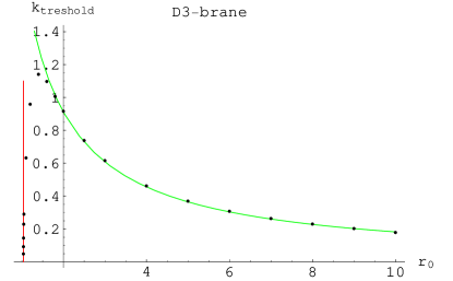
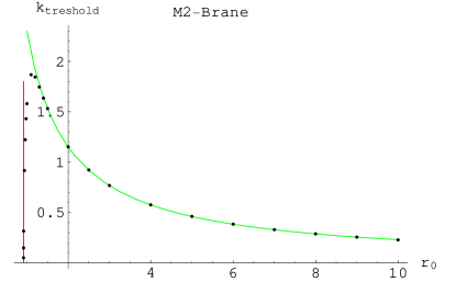
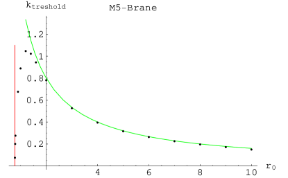
Figure 2: Instabilities of black D3, M2, and M5-branes. The dots represent threshold instabilities of the black branes we found. The vertical lines indicate the thermodynamic stability limits, which were found by (12), with $\tilde{R}=1$ for the D3-brane, $\tilde{R}=(1/3)^{1/6}$ for the M2-brane, and $\tilde{R}=(2/3)^{1/3}$ for the M5-brane. The curves indicate wavenumbers of threshold instabilities of uncharged black branes, with $r_{0}$ being the Schwarzchild radius.

Solving these linear ODE’s numerically, one extracts using a shooting algorithm the value of $k$ where a static perturbation exists, for any specified non-extremal mass. The results of this numerical investigation are summarized in figure 2. For large non-extremality, the threshold wavenumbers fit nicely onto the curve that gives those of an uncharged 3-brane. (This curve was obtained by reading off the wavenumber of the threshold instability of an uncharged 3-brane from the plots in [1, 2], and doing an appropriate scaling to get the values for an arbitrary $r_{0}$.) As one approaches the thermodynamic stability limit, the wavenumbers approach to zero. In fact, by zooming into this region, we were able to show that the wavenumbers go to zero approximately with a power-law behavior, with the critical exponent being close to $1/2$: that is, $k\sim\sqrt{r_{0}-r_{0}^{*}}$ where $r_{0}^{*}$ is the critical value where the instability disappears. Because $M$ is a non-singular function of $r_{0}$, one could also write $k\sim\sqrt{M-M_{*}}$. A naive way of understanding this is to think of some effective theory describing the perturbations in terms of a bosonic field with $m^{2}<0$. Then the criterion for the perturbations to be static is $\omega^{2}=k^{2}+m^{2}=0$, where $k$ is the wave-number of a static perturbation. The resulting equation, $k=\sqrt{-m^{2}}$, predicts the observed scaling, provided $m^{2}\sim r_{0}^{*}-r_{0}$. Such analytic behavior is a standard assumption: our argument basically amounts to a naive application of Landau theory.

The numerical stability analyses for the M2-brane and M5-brane are similar to the one for the D3-brane. The results are summarized in figure 2. Once again, near the thermodynamic stability limit, the wavenumbers go approximately as $\sqrt{r_{0}-r_{0}^{*}}$.

5 Conclusions

The stability of charged $p$-brane solutions was first attacked in [2]. Although the methods presented there are in principle practicable for any solution, they require considerable computational fortitude to apply. We have argued that a simple notion of universality classes is fairly broadly applicable to the question of brane stability: one commonly finds a thermodynamic relation $S\propto VT^{\alpha}$ for charged $p$-brane solutions in some limiting regime of parameters, and when one does, the stability properties depend only on $\alpha$—stability pertaining when $\alpha>0$. Given our treatment of the problem via a Kaluza-Klein reduction / truncation to a 2+1-dimensional action involving scalars and gravity, the dispersion relation of unstable modes would also appear to be the same for any solution in the universality class labeled by a given $\alpha$.

We have further shown, in section 4, that when one approaches a boundary of stability, the critical wavelength separating stable from unstable modes diverges, and that it does so for the cases studied with a critical exponent that could be guessed on the grounds of a naive effective field theory argument. It would be interesting to see if other exponents arise from non-generic situations, for instance a case where the temperature $T$ depends on mass as $T_{\rm max}-T\sim|M-M_{*}|^{\beta}$ for some $\beta\neq 2$. It is possible that spinning brane solutions provide a venue for more intricate thermodynamics [24, 25], but one would encounter there the complication of chemical potentials for the various angular momenta.

For the $p$-branes of type II string theory and M-theory, away from extremality but without angular momenta, thermodynamic stability pertains up to an upper mass limit given in equation (11). For the D3-brane, the M2-brane, and the M5-brane, our numerical analysis supports the claim [3, 4, 5] that dynamical and thermodynamic stability coincide. Extending the analysis to other $p$-branes should not be too difficult.

In conclusion, it seems that the notion of universality classes that we introduced in section 3, together with the behavior at a boundary of stability explored in section 4, represent a fairly comprehensive description of the qualitative features of the Gregory-Laflamme instability in linearized perturbation theory. Of course, it would be desirable to go beyond classical perturbation theory in understanding universality classes of behaviors for non-uniform horizons. Some of the methods of this paper may prove useful in that broader context as well.

References

- [1] R. Gregory and R. Laflamme, “Black strings and p-branes are unstable,” Phys. Rev. Lett. 70 (1993) 2837–2840, hep-th/9301052.
- [2] R. Gregory and R. Laflamme, “The Instability of charged black strings and p-branes,” Nucl. Phys. B428 (1994) 399–434, hep-th/9404071.
- [3] S. S. Gubser and I. Mitra, “Instability of charged black holes in anti-de Sitter space,” hep-th/0009126. To appear in the proceedings of Strings 2001.
- [4] S. S. Gubser and I. Mitra, “The evolution of unstable black holes in anti-de Sitter space,” JHEP 08 (2001) 018, hep-th/0011127.
- [5] H. S. Reall, “Classical and thermodynamic stability of black branes,” Phys. Rev. D64 (2001) 044005, hep-th/0104071.
- [6] G. T. Horowitz and K. Maeda, “Fate of the black string instability,” hep-th/0105111.
- [7] S. S. Gubser, “On non-uniform black branes,” hep-th/0110193.
- [8] B. Kol, “Topology change in general relativity and the black-hole black-string transition,” hep-th/0206220.
- [9] T. Wiseman, “Static axisymmetric vacuum solutions and non-uniform black strings,” hep-th/0209051.
- [10] T. Wiseman, “From black strings to black holes,” hep-th/0211028.
- [11] H. A. Chamblin and H. S. Reall, “Dynamic dilatonic domain walls,” Nucl. Phys. B562 (1999) 133–157, hep-th/9903225.
- [12] T. Hirayama, G.-w. Kang, and Y.-o. Lee, “Classical stability of charged black branes and the Gubser- Mitra conjecture,” hep-th/0209181.
- [13] T. Harmark and N. A. Obers, “Black holes on cylinders,” JHEP 05 (2002) 032, hep-th/0204047.
- [14] V. E. Hubeny and M. Rangamani, “Unstable horizons,” JHEP 05 (2002) 027, hep-th/0202189.
- [15] G. T. Horowitz and A. Strominger, “Black strings and P-branes,” Nucl. Phys. B360 (1991) 197–209.
- [16] G. T. Horowitz and J. Polchinski, “A correspondence principle for black holes and strings,” Phys. Rev. D55 (1997) 6189–6197, hep-th/9612146.
- [17] N. Itzhaki, J. M. Maldacena, J. Sonnenschein, and S. Yankielowicz, “Supergravity and the large N limit of theories with sixteen supercharges,” Phys. Rev. D58 (1998) 046004, hep-th/9802042.
- [18] S. S. Gubser, “Curvature singularities: The good, the bad, and the naked,” Adv. Theor. Math. Phys. 4 (2000) #3, hep-th/0002160.
- [19] K. Skenderis and P. K. Townsend, “Gravitational stability and renormalization-group flow,” Phys. Lett. B468 (1999) 46–51, hep-th/9909070.
- [20] D. Z. Freedman, S. S. Gubser, K. Pilch, and N. P. Warner, “Renormalization group flows from holography supersymmetry and a c-theorem,” Adv. Theor. Math. Phys. 3 (1999) 363–417, hep-th/9904017.
- [21] O. DeWolfe, D. Z. Freedman, S. S. Gubser, and A. Karch, “Modeling the fifth dimension with scalars and gravity,” Phys. Rev. D62 (2000) 046008, hep-th/9909134.
- [22] D. S. Salopek and J. R. Bond, “Nonlinear evolution of long wavelength metric fluctuations in inflationary models,” Phys. Rev. D42 (1990) 3936–3962.
- [23] D. J. Gross, M. J. Perry, and L. G. Yaffe, “Instability of flat space at finite temperature,” Phys. Rev. D25 (1982) 330–355.
- [24] M. Cvetic and S. S. Gubser, “Phases of R-charged black holes, spinning branes and strongly coupled gauge theories,” JHEP 04 (1999) 024, hep-th/9902195.
- [25] M. Cvetic and S. S. Gubser, “Thermodynamic stability and phases of general spinning branes,” JHEP 07 (1999) 010, hep-th/9903132.