M-Theory Moduli Space and Cosmology

Abstract

We conduct a systematic search for a viable string/M-theory cosmology, focusing on cosmologies that include an era of slow-roll inflation, after which the moduli are stabilized and the Universe is in a state with an acceptably small cosmological constant. We observe that the duality relations between different cosmological backgrounds of string/M-theory moduli space are greatly simplified, and that this simplification leads to a truncated moduli space within which possible cosmological solutions lie. We review some known challenges to four dimensional models in the “outer”, perturbative, region of moduli space, and use duality relations to extend them to models of all of the (compactified) perturbative string theories and 11D supergravity, including brane world models. We conclude that cosmologies restricted to the outer region are not viable, and that the most likely region of moduli space in which to find realistic cosmology is the “central”, non-perturbative region, with coupling and compact volume both of order unity, in string units.

I introduction

Cosmology offers a unique opportunity for testing string theory models. However, a prerequisite for taking advantage of this opportunity is a consistent framework that is not in obvious contradiction with basic known features about cosmology and particle phenomenology. This realization has revived interest in classifying time-dependent/cosmological string backgrounds and determining which class of solutions may be used to construct a viable string cosmology.

The growing flow of increasingly accurate data from cosmological observations, in addition to upcoming experiments with the power to discriminate between cosmological models offer the hope of guiding theory and confronting its predictions with accurate measurements. In particular, an epoch of primordial slow-roll inflationary evolution seems to be the simplest possible explanation for the existing data on cosmic microwave background (CMB) anisotropies and large scale structure observations (see for example, Bond:2002cg ); thus it is desirable to incorporate it into models of string cosmology (see, for example, Linde:2001qe ).

With this widespread interest in the predictions of string cosmology, one seems to be presented with a bewildering array of models to choose from, that seemingly could be shaped to fit any desirable results. However, there are well-known generic obstacles to obtaining slow-roll inflation, and to stabilizing moduli after inflation in a state with an acceptably small cosmological constant BS . These obstacles were originally discovered in the context of perturbative heterotic string theory, and could have been perceived as specific to that particular context. Since current cosmological models of other string theories, and braneworld scenarios based on them (see, for example, Quevedo:2002xw ; Ovrut:2002hi ) have gained popularity, it might have been assumed that in other string theories such problems are more easily overcome. However, the lesson of string duality is that there is a nice cohesion to the physics of string theory Polchinski . Dualities relate all the perturbative string theories and 11D supergravity (SUGRA). The strongly coupled limit of one particular theory, rather than being unknown, is something familiar, especially in the low energy limit described by SUGRA.

In this paper we will use the duality relations among the different corners of moduli space of supersymmetric vacua in string/M-theory to relate different models of string cosmology. We will be able to examine which regions of the moduli space lead to unsatisfactory cosmologies suffering from the aforementioned cosmological problems, and which regions may lead to promising cosmology. Our hope is that with this tool in hand, it will be easier to isolate and probe the sorts of background manifolds that will have the most promising behavior. Some preliminary progress in this direction has already been achieved center , and we use it to highlight the essential features of a viable string cosmology.

We should mention that the most detailed approach to constructing a consistent string cosmology is to give up on having a slow-roll phase of inflation and rather have “fast-roll” inflation in the pre-history of the Universe PBB . Fast-roll inflation is more sensitive to the details of the cosmological evolution, as opposed to the “no-hair” nature of slow-roll inflation. If the most recent period of inflation was of slow-roll type, then the preceding “pre-history” is hidden from us, so in this case it is sufficient to study cosmology from the last phase of slow-roll inflation and on, which is the attitude that we have adopted in this paper.

We begin in the next section by describing the action of duality in a cosmological context, making the observation that within the assumptions of string cosmology, the moduli space of solutions and the duality actions upon it greatly simplify. In section III, we divide the moduli space into “safe” regions where we trust perturbation theory, “unsafe” regions where we don’t, and a “central” region which is in some sense maximally unsafe. We then see how the different regions transform under duality, and make some preliminary arguments about physics in the central region. We continue in this section by looking at specific solutions to the cosmological equations of motion, and demonstrate how the various duality transformations act on these solutions. The explicit transformations can be found in the appendix. We conclude this section with a discussion of the physics of solutions in the outer region of moduli space.

In section IV, we extend our analysis to the case that there are non-perturbative potentials for the moduli, for example from brane instantons. Here we argue that the presence of potentials strengthens our argument for the importance of the central region. In section V we translate our analysis into the framework of various brane world cosmologies, and make some comments on the physics of these models. In section VI we briefly discuss cosmology in the central region, summarizing the argument made in center , and we end with some conclusions and future directions in section VII.

II string cosmology and duality

We begin this section by explicitly stating the assumptions on which we base our approach to string cosmology. We shall continue by looking at how string duality transformations work within these assumptions, giving simple, explicit transformations that we can apply to cosmological solutions.

We are interested in finding cosmological solutions of String/M-theory that will describe homogeneous and isotropic 4 dimensional space-times. Our primary interest will be to isolate any solutions that produce a slow-roll inflationary era ending with stabilized moduli in a universe with an acceptably small cosmological constant. Of course, these solutions will also have the usual extra, compact dimensions, which are necessary for the consistency of the theory. Although we are far from having satisfactory control over the full, non-perturbative completion of string theory, we know that its low energy effective field theory should be described by SUGRA. In particular, the energy scale of reasonable inflaton potentials responsible for slow-roll inflation is generally far smaller than the Planck scale. SUGRA should therefore describe the cosmological evolution very well throughout an inflationary era and for all but the very highest curvatures.

What differentiates our analysis from a pure SUGRA analysis, however, is that we always have in mind a derivation from string theory. Thus, we only trust our solutions when we trust their stringy completion. In particular, we trust our solutions only when they correspond to a string background with small string coupling and low string-frame space-time curvature.

There are three key features exhibited by such stringy cosmological solutions. The first is that string theory phenomenology prefers the use of SUGRA for the low energy effective theory, rather than simple gravity, and we are forced to address the problem of moduli such as the dilaton. Any regions where we trust perturbative string theory will have these moduli, and in particular we must deal with the well known instability, first elucidated by Dine and Seiberg DS , which drives perturbative strings to the free, noncompact limit, and its cosmological counterpart BS . Many studies of string cosmology make the assumption that there is a non-perturbative mechanism for stabilizing moduli whose effects on cosmological physics are subsequently ignored. In this work, instead, we find that the mechanism of moduli stabilization can be a natural source for realistic, slow-roll inflation. A second feature is that since we have forced ourselves to accept some of the difficulties of string theory, and have been careful that the embedding is justified, when the solution drives the Universe towards a state with high energy densities, we will assume that in some cases string theory can make some sense of it. Finally, we note that by embedding our solutions in the framework of string theory, we can use string dualities to our advantage. The structure of the moduli space of string theory supplies our model with a valuable framework, within which we can exercise greater control over the necessary approximations. In particular, if the gravity solution goes to a strong-coupling or strong (compact) curvature regime, we can use string duality to map our solution to a different solution whose physics is often well-controlled.

In this paper we focus on Einstein gravity coupled to scalar moduli fields in 4 space-time dimensions. In general, these fields are imbedded within an $N=1$ SUGRA theory, whose full form is dictated by string theory. Most of the details of the SUGRA theory are unimportant for cosmology, apart from a possible scalar potential, whose effects we will consider in section IV. Thus we use the simple lagrangian:

$$S_{4}=\frac{1}{2\kappa_{4}^{2}}\int d^{4}x\sqrt{-g}[R-\frac{1}{2}g^{\mu\nu}\partial_{\mu}\phi\partial_{\nu}\phi-\frac{1}{2}g^{\mu\nu}\partial_{\mu}\sigma\partial_{\nu}\sigma-V(\phi,\sigma)]\quad.$$ (1)

The fields $\phi$ and $\sigma$ are two representative moduli fields that control the string coupling and, in our example, the size of the compact space. This restriction on models comes about because we are interested in spatially homogeneous and isotropic 4 dimensional spacetimes. The scalar moduli serve as the most likely inflaton candidates in string cosmology BG .

Recall that the action (1) is a restriction of the full low-energy effective SUGRA action. As such, it inherits dualities from the full string theory. There is, of course a menagerie of S, T, and U string dualities, as well as M-theory strong coupling limits where the space-time grows extra dimensions. These different dualities have very distinct and specific actions on string states that can be very complicated. When restricted to dilaton gravity, however, the dualities simplify considerably. For example, we may consider T-duality, which depends crucially on the string winding states that are interchanged with Kaluza-Klein modes along the compact directions. Since our cosmological models have no need to pay attention to the detailed dynamics of momentum or winding states, the only effect of T-duality is an inversion of the size of the compactification and a shift in the dilaton. Likewise, the evidence for S-duality rests largely on the behavior of the spectrum of BPS states, which are irrelevant for cosmology. Thus, general duality transformations can be applied in a simplified way to extend the range of trustworthy solutions, a procedure we shall now illustrate in more detail. Dualities were discussed in the context of string cosmology in coprev , with emphasis on the symmetries of cosmological solutions of a single low energy effective action. Here our focus is on the relations between cosmological solutions of different string theories.

Our 4D lagrangian comes from a dimensional reduction of the 10D action. Restricting ourselves to the gravity plus dilaton sector of the theory, all of the low energy effective actions for the different perturbative string theories reduce to the same simple form:

$$S_{10}=\frac{1}{2\kappa_{10}^{2}}\int d^{10}x\sqrt{-G}e^{-2\Phi}\left(R_{10}+4G^{MN}\partial_{M}\Phi\partial_{N}\Phi\right)\quad,$$ (2)

where $G_{MN}$ is the ten dimensional string-frame metric of the corresponding string theory, and $\Phi$ is the ten dimensional dilaton of that theory. For simplicity, we shall initially assume that 6 directions are toroidally compactified. We shall make some comments below about the behavior we expect for more complicated compactification manifolds. In particular, a more realistic compactification manifold will determine the form of the lower dimensional superpotential.

After reducing this action on a torus of compact volume $V$, and redefining fields to get to the four dimensional Einstein frame, we recover the four dimensional action (1), with the lower dimensional fields related by

$$\phi = \Phi$$ (3)

$$ds_{10}^{2}=G_{MN}dx^{M}dx^{N} = e^{\frac{1}{2\sqrt{3}}\sigma+\frac{1}{2}\phi}(e^{-\frac{2}{\sqrt{3}}\sigma}g_{\mu\nu}dx^{\mu}dx^{\nu}+g^{c}_{mn}dy^{m}dy^{n})$$ (4)

$$\kappa_{4}^{2} = \frac{\kappa_{10}^{2}}{V_{6}}=\frac{\kappa_{10}^{2}}{\int d^{6}y\sqrt{g^{c}}}\quad,$$ (5)

where $g^{c}_{mn}$ is a flat, compact metric on the six-torus parameterized by $y^{m}$, whose volume $V_{6}$ is string-scale. The 4D dilaton is $\phi$, and $\sigma$ controls the proper size of the compact manifold. Note that the lower-dimensional action is invariant under $SO(2)$ rotations between $\phi$ and $\sigma$. Because of this, there is some freedom of choice in the definition of the four-dimensional fields. We have chosen the fields such that the duality relations for the ten-dimensional fields translate into simple transformations of the four-dimensional fields. In this paper, we will be concerned with three varieties of duality transformation: S-dualities, T-dualities, and “M-theory limits”, whose action we shall now outline.

The S-duality transformation comes from the stringy strong-weak coupling S-dualities, i.e. those between the heterotic and type I strings, or the strong-weak part of the type IIB $SL(2,Z)$ self-duality. These dualities operate on the ten-dimensional and string frame metric by, for example,

$$G^{I}_{MN} = e^{-\Phi_{h}}G^{h}_{MN}$$ (6)

$$\Phi_{I} = -\Phi_{h}$$ (7)

for the type I and heterotic fields, with a similar action occurring in the type IIB string. The lower dimensional action thus inherits a transformation:

$$\phi\rightarrow-\phi$$ (8)

$$\sigma\rightarrow\sigma\quad.$$ (9)

Note that the S-duality transformations never change the 4 dimensional Einstein frame metric. We can use these transformations to choose $\phi\leq 0$, which implies $g_{s}\leq 1$.

The second type of transformation we shall consider are T-duality transformations, which for simplicity we shall take to act on the entire 6-torus:

$$G_{c}\equiv e^{\frac{1}{2\sqrt{3}}\sigma+\frac{1}{2}\phi}g_{c}\rightarrow G_{c}^{-1}$$ (10)

$$\Phi\rightarrow\Phi-\frac{1}{2}\log\det G_{c}\quad,$$ (11)

which translates into

$$\phi\rightarrow-\frac{1}{2}\phi-\frac{\sqrt{3}}{2}\sigma$$ (12)

$$\sigma\rightarrow-\frac{\sqrt{3}}{2}\phi+\frac{1}{2}\sigma\quad.$$ (13)

This transformation can be used to choose the combination $\frac{1}{2\sqrt{3}}\sigma+\frac{1}{2}\phi\geq 0$, which causes the compact torus directions to have proper length greater than or equal to the string length.

The final type of transformation we will consider is the “M-theory limit”. This limit will be most useful when we are considering models corresponding to compactifications of the heterotic $E8\times E8$ string, although it will also apply to models derived in the type IIA theory. In solutions where we find the 10 dimensional string coupling growing large, we expect the 11th dimension of heterotic M-theory to open up. In the compactified theory, this should then look like a 5th dimension opening up. This is more or less the type of solution that one deals with in brane world scenarios as well as in the Ekpyrotic scenario Ekp1 ; Ekp2 . A solution of the four dimensional action maps into a 5 dimensional solution of the Einstein-Hilbert action, coupled to a 5 dimensional scalar field $\sigma_{5}$, if we identify the 5 dimensional metric and scalar according to:

$$ds_{5}^{2} = e^{-\frac{1}{2}\phi-\frac{1}{2\sqrt{3}}\sigma}g_{4\mu\nu}dx^{\mu}dx^{\nu}+e^{\phi+\frac{1}{\sqrt{3}}\sigma}dz^{2}$$ (14)

$$\sigma_{5} = \frac{\sqrt{3}}{2}\sigma-\frac{1}{2}\phi\quad.$$ (15)

The 5 dimensional form has been defined so that the coordinate $z$ is the same one used in the usual $10\rightarrow 11$ dimensional M-theory decompactification limit, which we recall takes the form:

$$ds_{11}^{2}=e^{-\frac{2\Phi}{3}}G_{10MN}dx^{M}dx^{N}+e^{\frac{4\Phi}{3}}dz^{2}\quad.$$ (16)

We will also want to pay attention to the 11D metric corresponding to a given 4D metric, dilaton, and $\sigma$-field:

$$ds_{11}^{2}=e^{\frac{1}{2\sqrt{3}}\sigma-\frac{1}{6}\phi}(e^{-\frac{2}{\sqrt{3}}\sigma}g_{\mu\nu}dx^{\mu}dx^{\nu}+g^{c}_{mn}dy^{m}dy^{n})+e^{\frac{4}{3}\phi}dz^{2}\quad.$$ (17)

Note that, while before we chose the compact directions $y^{m}$ to be string scale, here we must choose the coordinate $z$ to be of order the 11D Planck length $e^{\phi/3}l_{s}$, for the tower of Kaluza-Klein states to correctly reproduce the spectrum of D0-brane bound states. Requiring both the 11th dimension and the six compact dimensions to be larger than the 11D Planck length becomes the requirement that $\phi>0$ and $\frac{1}{4\sqrt{3}}\sigma-\frac{5}{12}\phi>0$, or $\sigma>\frac{5}{\sqrt{3}}\phi>0$.

Since the dilaton plus gravity effective action of all perturbative string theories has the same functional form, the action of dualities on the different effective actions has to be represented by field redefinitions which are allowed by the symmetries of the lagrangian. The duality transformations must therefore act on the space of solutions by mapping one set of solutions onto another set. We will develop these mappings in the following section.

Note that in general these duality relations are seen in backgrounds with extended SUSY, such as the toroidal compactifications we are presently studying. However, we expect similar relations to continue to hold at the level of the $N=1$ SUGRA models that we need for a realistic particle phenomenology. For example, although it is difficult to describe explicitly for Calabi-Yau manifolds, our string intuition states that if the volume modulus shrinks, then various winding states will become light, and that the appearance of these states can then be treated by looking at a different effective compactification which has a large compact volume. Considering more realistic $N=1$ SUSY compactifications in our effective field theory allows non-perturbative superpotentials for the moduli, whose features we will investigate in section IV.

III Outer region solutions without potential

For regions of our simplified moduli space that have large compact directions (compared to the string scale) and small string coupling, we trust the string derivation of the low energy effective field theory action; this is what we will generically call the “safe” region of moduli space If we find ourselves with $g_{s}\gg 1$, or a compactification direction $R\ll l_{s}$, we can apply an S or T duality to map it to one of the safe regions. Those parts of moduli space that can be mapped to a safe region by a duality transformation we will call the outer region of moduli space.

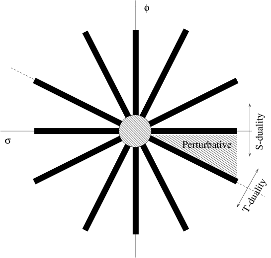
Figure 1: Regions of string moduli space. The shaded circular region is the “central” region and the dark rays indicate regions in which one of the moduli is perturbative while the other is not. The region marked “perturbative” is the fully perturbative region and the white wedges between the rays are its images under duality.

Figure 1 shows the perturbative region and its images under different dualities for backgrounds that exhibit S-duality. The ray along the $\phi$ axis depicts the region in which $\sigma$ is approximately fixed such that the compact volume is of order the string volume and the coupling is perturbative for some background. The ray along the $\sigma$ axis depicts the region in which $\phi$ is approximately fixed such that the string coupling is of order one and the compact volume is larger than the string volume for some background. The other rays can be thought of as their images under duality. Note that along the $\sigma$ axis, for example, we expect to be able to use four-dimensional $N=1$ SUGRA with one dynamical field $\phi$ to study cosmology. However, we do not have a way to derive the effective action in a trustworthy manner from M-theory. Thus to study cosmology in this region of moduli space we choose to parameterize it by a chiral superfield of $D=4$, $N=1$ SUGRA.

The regions with both $g_{s}\sim 1$ and $R\sim l_{s}$, which cannot be mapped to a safe region for either modulus by applying a duality transformation is called the “inner” (or “central”) region, and it is where we expect the general principles of string universality to apply bda1 . Again, we expect to be able to use $N=1$ SUGRA in studying cosmology here, although we lack a way to derive the effective action systematically from M-theory. Thus to study cosmology in the central region of moduli space we generally parameterize it by several chiral superfields of D=4, $N=1$ SUGRA. We assume, along the lines of bda2 , that they are all stabilized at the string scale by stringy non-perturbative (SNP) effects which allow a continuously adjustable constant in the superpotential. SUSY is broken at an intermediate scale by field theoretic effects that shift the stabilized moduli only by a small amount from their unbroken minima. The cosmological constant can be made to vanish after SUSY breaking by the adjustable constant.

In the rest of this section, we explicitly exhibit the duality relations that can be used to map “unsafe” region solutions of the outer region to “safe” regions, which allows us to get a grasp on the cosmological behavior of any model in the outer region. With this we will be able to argue that realistic slow-roll inflationary cosmology must, within our general assumptions, necessarily occur in the (relatively quite small) central region of our simplified moduli space.

An important caveat to mention is that our knowledge of the behavior within moduli space is more complete in those models exhibiting S-duality. In particular, the picture of calculable regions within moduli space for models with M-limits is as shown Figure 2. There is a large region where the dilaton is large enough that we need to use the 11D theory, but also in which the 6 compact dimensions are smaller than the 11D Planck length. Lacking any analog of T-duality for membrane states, we end up with a larger unsafe region than just the central region of interest. Perhaps this region can still be parametrized by a 5D SUGRA, so some general conclusions might still be made. In any case, we will later see that membrane instantons lead to an instability analogous to the Dine-Seiberg instability, and thus that we are once again forced to consider the central region once we allow for scalar potentials. It should be noted, however, that knowledge of the general behavior of potentials for M-theory limits is not as complete as it is for the perturbative string backgrounds.

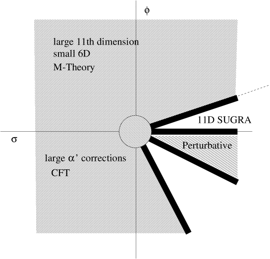
Figure 2: Regions of M-theory moduli space. The shaded circular region is the “central” region and the dark rays indicate regions in which one of the moduli is perturbative while the other is not. The region marked “perturbative” is the fully perturbative region. Other regions are marked accordingly: the wedge where 11D SUGRA is valid, the shaded region in which the full quantum M-theory needs to be used, and the region in which classical string theory is valid and $\alpha^{\prime}$ corrections are large. The unmarked wedge is T-dual to the perturbative region

As explained previously, in terms of the SUGRA fields of the low energy theory the duality transformations correspond to trivial field redefinitions, which are allowed by the symmetries of the lagrangian. However, we should always keep in mind that the model is derived from a more fundamental string theory. Because of the duality relations, any solution in the outer region can be derived in a trustworthy manner from some perturbative string theory, within which solutions are well known and offer very few possibilities for surprises.

We begin by investigating models with 4 dimensional flat cosmologies, and a time dependent dilaton, which will capture the essential physics of any outer region cosmologies without potentials. We will use the Friedmann-Robertson-Walker (FRW) ansatz for the non-compact space:

$$ds_{4}^{2} = -dt^{2}+a^{2}(t)dx^{i}dx^{i}$$ (18)

$$\phi = \phi(t)\quad.$$ (19)

With this ansatz for the fields, and with our fields normalized as in eq.(1) we find the equations of motion:

$$H^{2} = \frac{1}{6}\rho$$ (20)

$$\dot{H} = -\frac{1}{4}(\rho+p)$$ (21)

$$\ddot{\phi}+3H\dot{\phi} = 0\quad,$$ (22)

where

$$H = \dot{a}/a$$ (23)

$$\rho = p=\frac{1}{2}\dot{\phi}^{2}\quad.$$ (24)

The cosmological solutions to these equations are simple and well known,

$$a(t) = a(1)|t|^{1/3}$$ (25)

$$\phi(t) = \phi(1)\pm\frac{2}{\sqrt{3}}\ln|t|\quad,$$ (26)

where we have placed the inevitable singularity in the solution at $t=0$ for convenience. Of course, the solutions cannot be trusted in regions where the string coupling is of order unity and the curvature is high.

These well-known solutions naturally break up into four different cases, depending on the sign chosen in the solution for $\phi$, and on whether the singularity in $t$ lies to the future or to the past. In the Pre-Big Bang (PBB) scenario, and in the Ekpyrotic scenario, a transition between the different branches is envisioned in a single cosmology of the same string theory. We, on the other hand, consider duality relations that map solutions (whether they include a transition between the branches or not) onto other well controlled solutions of (in general) another string theory.

Figure 3: Action of S-duality on cosmological solutions of different string theories. The solutions have the same form in each theory, and the arrow labeled “S-duality” indicates how they are related. For example, the contracting $(+)$ solution in one theory is mapped onto the contracting $(-)$ solution of the S-dual theory.

In this simple first case, we can apply either S-duality transformations or M-theory limits. The S-duality transformation will apply for a model that is derived from type IIB, type I, or Heterotic $SO(32)$ string theories, and simply reverses the sign of the dilaton according to eqs.(8),(9), leaving the metric unchanged. Thus it simply exchanges the ‘$+$’ and ‘$-$’ branches of the solutions of the two dual theories. The “pool” of solutions to choose from in any of the theories is the same pool for all theories. For models derived from the Heterotic $E8\times E8$ or type IIA theories, our solutions map into 5-dimensional solutions, using eqs. (14), (15)

$$ds_{5}^{2} = e^{-\frac{\phi(1)}{2}}|t|^{\pm\frac{1}{\sqrt{3}}}(-dt^{2}+a^{2}(1)|t|^{\frac{2}{3}}dx^{i}dx^{i})+e^{\phi(1)}|t|^{\pm\frac{2}{\sqrt{3}}}dz^{2}$$ (27)

$$\sigma_{5} = -\frac{1}{2}\phi(1)\mp\frac{1}{\sqrt{3}}\ln|t|\quad,$$ (28)

where $\sigma_{5}$ is a massless scalar in 5D. One can easily check that this is a solution of the 5-dimensional equations of motion.

We would like to point out that the 5D solution space is isomorphic to the 4D solution space, and therefore 4D solutions can be mapped onto 5D solutions and vice-versa. Properties of solutions can be studied in either the 4D or the 5D setup. The 5D solution is relevant for compactifications that have a strong coupling limit described in terms of 11D SUGRA.

We make the following almost trivial observations:
$(i)$ Solutions (25), (26) do not describe slow-roll inflation at any time, since they obey $\dot{H}\sim H^{2}$. They can describe a period of accelerated contraction as in the PBB scenario, which could be interpreted as “fast-roll” inflation.
$(ii)$ Obviously, the moduli are not stabilized wherever equations (25) and (26) are valid.
$(iii)$ As the solution approaches the central region it ceases to be valid and new interaction terms in the effective action are expected to kick in.
These conclusions are valid for 4D solutions as well as for 5D solutions, where they are interpreted as the motion of branes in a 5D universe.

We can now relax our restrictions somewhat, and consider the case with two moduli. We will consider one modulus, $\phi$, controlling the coupling, while the other, $\sigma$, controls the size of the compact manifold through our ansatz (4) for the 10D metric. We now have an additional equation of motion,

$$\ddot{\sigma}+3H\dot{\sigma}=0\quad,$$ (29)

and now

$$\rho=p=\frac{1}{2}\dot{\phi}^{2}+\frac{1}{2}\dot{\sigma}^{2}\quad.$$ (30)

The 4D solutions now take the more general form

$$a(t) = a(1)|t|^{\frac{1}{3}}$$ (31)

$$\phi(t) = \phi(1)+p_{\phi}ln|t|$$ (32)

$$\sigma(t) = \sigma(1)+p_{\sigma}ln|t|\quad,$$ (33)

with the algebraic constraint

$$p_{\phi}^{2}+p_{\sigma}^{2}=\frac{4}{3}\quad.$$ (34)

For weak coupling and low string-curvature solutions, we require $\phi<0$ and $\frac{1}{2\sqrt{3}}\sigma+\frac{1}{2}\phi>0$, and we find ourselves in the central region when $\sigma,\phi\sim 0$. Note that, apart from some simple mixing between $\phi$ and $\sigma$ as sources, the dynamics is identical to the single modulus case, in that there will be solutions looking like either the ‘$+$’ or ‘$-$’ branches considered previously, and that they can be studied equivalently in their 4D or 5D versions, as we show below.

As in the single field case, we note that solutions (31), (32), and (33) do not describe slow-roll inflation at any time, but they can describe a period of accelerated contraction as in the PBB scenario, that moduli are not stabilized while (31), (32), and (33) are valid, and that as the solution approaches the central region it ceases to be valid and new interaction terms in the effective action are expected to kick in.

A detailed study of such solutions and their generalizations has been conducted for many specific cases: PBB, heterotic M-theory, Ekpyrotic scenario, etc. Our aim here is to show that the classification of solutions in the outer region is complete and that there are no new features coming from any particular microscopic dynamics that one may wish to invoke in the outer region.

Now that we have a two moduli set-up, we can also look at the action of T-duality on the solutions. The only real issue is to pay attention to when a given solution is in the outer region, and when it is in the central region.

Let’s first look at the case of models derived from type IIB, type I, or Heterotic $SO(32)$ strings. As argued previously on general grounds, since the action for these theories is of the same form, and therefore the spaces of solutions of the theories are isomorphic, dualities must have a representation on the space of solutions. For this particular case the 4D solutions are mapped to other 4D solutions under S-duality by

$$\phi(1)\rightarrow-\phi(1)$$ (35)

$$p_{\phi}\rightarrow-p_{\phi}\quad,$$ (36)

and $\sigma$ is unchanged. Under T-duality the solutions undergo a more complicated transformation

$$p_{\phi}\rightarrow-\frac{1}{2}p_{\phi}-\frac{\sqrt{3}}{2}p_{\sigma}$$ (37)

$$p_{\sigma}\rightarrow-\frac{\sqrt{3}}{2}p_{\phi}+\frac{1}{2}p_{\sigma}\quad,$$ (38)

with an identical action holding on the integration constants $\phi(1)$ and $\sigma(1)$. These are clearly still solutions, since

$$(-\frac{1}{2}p_{\phi}-\frac{\sqrt{3}}{2}p_{\sigma})^{2}+(-\frac{\sqrt{3}}{2}p_{\phi}+\frac{1}{2}p_{\sigma})^{2}=p_{\phi}^{2}+p_{\sigma}^{2}\quad.$$ (39)

Notice that despite the very similar form, this transformation is very different from the one induced by “Scale-factor-duality” SFD which is a symmetry of the equations of motion for cosmological solutions under which solutions are mapped onto other solutions of the same string theory, while dualities map solutions of one string theory onto solutions of the dual string theory.

The two moduli solutions that we have found can be explicitly mapped to 5D, 10D, and 11D solutions, as we show below and in the appendix. It is the 10D form of the solution that determines whether we trust string perturbation theory; when the string frame curvature is small in string units, the compact directions are large compared to the string scale, and the string coupling is small, we can follow the evolution with confidence. The 5D solution is of interest whenever all relevant length scales are much larger than the 5D Planck scale, giving us a 5D interpretation of cosmology, and the 11D solution is of interest when it is trustworthy in 11D SUGRA.

We will discuss explicitly the 5D case appropriate for studying braneworld models, and relegate the other examples to Appendix A. For the 5D case we have Einstein gravity coupled to one scalar $\sigma_{5}$ as in eqs.(14,15). In this case the map into 5D solutions is the following:

$$ds_{5}^{2} = C_{5}^{2}|t|^{-\frac{1}{2\sqrt{3}}p_{\sigma}-\frac{1}{2}p_{\phi}}(-dt^{2}+a^{2}(1)|t|^{\frac{2}{3}}dx^{i}dx^{i})+C_{5}^{-4}|t|^{\frac{1}{\sqrt{3}}p_{\sigma}+p_{\phi}}dz^{2}$$ (40)

$$\sigma_{5} = \frac{\sqrt{3}}{2}\sigma(1)-\frac{1}{2}\phi(1)+(\frac{\sqrt{3}}{2}p_{\sigma}-\frac{1}{2}p_{\phi})\ln{|t|}$$ (41)

$$C_{5} = e^{-\frac{1}{4\sqrt{3}}\sigma(1)-\frac{1}{4}\phi(1)}\quad.$$ (42)

These become, after rescaling the time variable by $dt_{5}=C_{5}|t|^{-\frac{1}{4\sqrt{3}}p_{\sigma}-\frac{1}{4}p_{\phi}}dt$,

$$ds_{5}^{2} = -dt_{5}^{2}+a_{5}^{2}(1)|t_{5}|^{2p_{5a}}dx^{i}dx^{i}+c_{5}^{2}(1)|t_{5}|^{2p_{5c}}dz^{2}$$ (43)

$$\sigma_{5} = \sigma_{5}(1)+p_{5\sigma}\ln{|t_{5}|}\quad.$$ (44)

More details can be found in the appendix.

To summarize the behavior of the outer region solutions, we note that such solutions do not describe slow-roll inflation; when they are valid the moduli are not stabilized and they become invalid as they approach the central region. This holds for 4D solutions and for their 5D counterparts. Our conclusions are the following

1. It does not seem to be possible to construct a viable cosmology which evolves entirely in the outer region.

2. Slow-roll inflation is likely to be obtained only when moduli are in the central region.

In the next section we will show that these conclusions are not likely to be altered when potentials for the moduli are included.

IV Cosmology with moduli potentials

The moduli potential is an important ingredient in any string theoretic cosmological scenario, and it is particularly important when looking for scenarios that involve an epoch of slow-roll inflation. We will treat this in the same spirit as the rest of the paper: we look for moduli potentials that are either derived from string theory, in cases where the derivation is trustworthy, or that are constrained by general arguments and symmetries when such a derivation is not available. In addition, we consider constraints coming from the requirement of moduli stabilization in a minimum with an acceptably small cosmological constant, in which moduli can end up after the inflationary epoch. This turns out to impose rather severe restrictions on models. We will continue to consider theories that are imbedded in $N=1$ SUGRA.

In the context of weakly coupled heterotic string theory it is well known that the potentials that are generated for the dilaton and the compactification moduli are typically of the runaway form DS so that the theory prefers to go to the zero coupling and decompactification limit. Similar problems are encountered in theories in which SUSY is broken completely by string theoretic effects, such as the Scherk-Schwarz mechanism where the compactification explicitly breaks SUSY. In addition, the generated potentials are steep BS , and consequently have a problem providing enough slow-roll inflation. We will use dualities to extend these arguments to all corners of moduli space. Additionally, we will include the contributions of brane instantons. In the next section models of brane annihilation, tachyon condensation, and Ekpyrosis will be discussed and the problems with such scenarios will be highlighted.

We focus on non-perturbative potentials, since it is well-known that perturbative potentials have problems in satisfying the generic phenomenological requirements as above. Non-perturbative sources for moduli potentials originate from field theoretic effects and stringy non-perturbative effects (SNP). Field theoretic effects such as hidden sector gaugino condensation gaugino1 ; gaugino2 have been discussed previously very extensively (see, for example, Nilles:1998uy ), so we will not repeat the discussion here. The SNP that we will consider originate from brane-instanton effects.

General arguments based on Peccei-Quinn symmetries, and how they break due to non-perturbative effects, show that the superpotential must be a sum of exponentials in the moduli. These exponentials can be generated by either stringy or field theoretic non-perturbative effects. A constant term in the superpotential is allowed by the symmetries but has no natural mechanism for its generation.

In the last few years there have been attempts to stabilize moduli using various fluxes in the internal space (see for example gkp ). However all these arguments ignore the back reaction of the flux on the internal space and it appears that when this is taken into account the derivation of the potential for the moduli becomes invalid. A detailed discussion of the problems associated with potentials from fluxes is currently under preparation by one of the authors (SdA). In any case, even according to these discussions the volume modulus is not stabilized, so that one would still be forced to consider SNP effects. Also these potentials are qualitatively similar to those generated by gaugino condensation (i.e. the so-called race-track models kras ; deCarlos:1992da ; Dine:1999dx ) and hence will have the same cosmological problems as those highlighted in BS .

To some extent the results of this section are contained explicitly or implicitly in the existing literature, but we will state them explicitly to substantiate our arguments.

IV.1 Non-perturbative moduli potentials

Even in the absence of SUSY breaking one would expect SNP effects coming from the various brane instantonsbda1 ; ovrut ; moore . Our goal is to determine their influence on cosmological solutions. Brane instantons are Euclidean configurations that are obtained by wrapping the extended directions of a brane, including its Euclidean time direction, around some cycle in the compact space. Their action is the product of the brane tension and the volume of the cycle around which its world volume is wrapped. Since under dualities BPS branes transform into BPS branes, brane instanton SNPs in one string theory (or 11D SUGRA) transform into SNPs in the other theory.

For example, in the case of the M-limit transformation between the heterotic $E_{8}\times E_{8}$ (HE) theory and its strong coupling version the Horava-Witten (HW) theory, the non-perturbative effects due to the fundamental string and the NS fivebrane instantons tend to give a runaway dilaton potential which makes the dilaton roll down to weak coupling, whereas in the HW theory the corresponding dual effect originates from the M two-brane and M five-brane instantons which tend to push the theory towards infinite radius for the eleventh dimension, i.e. to strong coupling. In terms of the dilaton, these effects are competing and it is thus plausible to have it stabilized around zero, where neither perturbative heterotic strings nor 11D supergravity can describe the physics.

Note that an additional effect of the M-brane instantons for the two-modulus case is to drive the 6 compact directions $y_{m}$ to large radius as well. However, as illustrated in Figure 2, there is a larger region of moduli space for “M-limit” theories that are not accessible to direct calculation. We are thus unable, without a more detailed treatment of the superpotential, to exhibit the competing effects that would stabilize a second modulus like the $\sigma$ field.

As in the previous sections we focus for simplicity on toroidally compactified theories and we therefore have two moduli: $\phi$, which controls the string coupling,

$$g=e^{\phi}\quad,$$ (45)

and $\sigma$, which controls the compactification radius,

$$R/l_{S}=e^{\frac{1}{4\sqrt{3}}\sigma+\frac{1}{4}\phi}\quad.$$ (46)

For the M-limit case, when an extra dimension opens up the radius of the 11th dimension obeys

$$\rho/l_{11}=e^{\frac{2}{3}\phi}\quad,$$ (47)

and the other six compact dimensions have radius

$$R/l_{11}=e^{\frac{1}{4\sqrt{3}}\sigma-\frac{5}{12}\phi}\quad.$$ (48)

In accordance with the general arguments about the dependence of SNP on moduli, it was found that SNP effects depend exponentially both on the compact volume $V_{6}$ and on either $1/g$ or $1/g^{2}$. In the outer region of moduli space dominant SNP come from two or sometimes three BPS branes, whose instanton actions have the weakest dependence on the string coupling $g$, and compactification radius $R$, or their product. A list of such BPS branes and their instanton actions is given in Table 1. The notation is taken from bda1 .

	Type I		HO
	brane	action	brane	action
	$D5$	$\frac{1}{g_{I}}\left(\frac{R}{l_{I}}\right)^{6}$	$F5$	$\frac{1}{g_{HO}^{2}}\left(\frac{R}{l_{HO}}\right)^{6}$
	$D1$	$\frac{1}{g_{I}}\left(\frac{R}{l_{I}}\right)^{2}$	$F1$	$\left(\frac{R}{l_{HO}}\right)^{2}$
	HE		HW
	brane	action	brane	action
	$F5$	$\frac{1}{g_{HE}^{2}}\left(\frac{R}{l_{HE}}\right)^{6}$	$M5$ transverse	$\left(\frac{R}{l_{11}}\right)^{6}$
	$F1$	$\left(\frac{R}{l_{HE}}\right)^{2}$	$M2$ longitudinal	$\left(\frac{R}{l_{11}}\right)^{2}\frac{\rho}{l_{11}}$
	IIA		MS1
	brane	action	brane	action
	$D0$	$\frac{1}{g_{IIA}}\frac{R}{l_{IIA}}$	$KK$ graviton	$\frac{R}{\rho}$
	$F1$	$\left(\frac{R}{l_{IIA}}\right)^{2}$	$M2$ longitudinal	$\left(\frac{R}{l_{11}}\right)^{2}\frac{\rho}{l_{11}}$
	IIA		IIB
	brane	action	brane	action
L	$D0$	$\frac{1}{g_{IIA}}\frac{R_{IIA}}{l_{II}}$	$D\!-\!1$	$\frac{1}{g_{IIB}}$
T	$D0$	$\frac{1}{g_{IIA}}\frac{R}{l_{II}}$	$D1$	$\frac{RR_{IIB}}{g_{IIB}l_{II}^{2}}$
L	$F1$	$\frac{RR_{IIA}}{l_{II}^{2}}$	$KK$ MM	$\frac{R}{R_{IIB}}$
T	$F1$	$\frac{R^{2}}{l_{II}^{2}}$	$F1$	$\frac{R^{2}}{l_{II}^{2}}$

Table 1: Dominant BPS branes and their instanton actions taken from bda1 .

In the table, $Dn$ refers to a D-brane instanton with an $n+1$-dimensional world-volume in the appropriate theory. Similarly $F1$ and $F5$ refer to instantons for the fundamental string or NS 5-brane wrapping 2D or 6D volumes, respectively. Longitudinal and transverse refer to whether or not the brane wraps the M-limit direction. In the portion of the table with instantons for the type IIA and type IIB branes, the two backgrounds are related by T-duality in a preferred direction. The entries marked $L$ and $T$ refer to wrappings that are longitudinal or transverse with respect to this preferred coordinate. $KK$ MM stands for Kaluza-Klein momentum mode. The size of a direction that is not T-dualized is denoted $R$. Unlike the previous cases of S-duality, we have to make a distinction between different radii, since even if their sizes were equal to begin with, the T-duality changes them.

To determine cosmology in the outer region of moduli space it is enough to consider only a few contributions. The (super)potentials induced by brane instantons, in the approximation that we will use, ignoring the prefactor and questions related to fermion zero modes, are simply given by $V\sim e^{-{\rm action}}$.

Note that in terms of our scalars $\phi$ and $\sigma$, the brane instanton potentials are exponentials of exponentials in the moduli fields, for example, $V\sim e^{-e^{-\phi}}$. Duality acts on cosmological equations of motion with a potential induced by SNP in one background by mapping into the equations of another theory, as in the case without potentials. Therefore solutions in one theory have to be mapped onto solutions of the other theory. The exact form of the solutions cannot be obtained analytically, but their general properties are quite similar to the no-potential case.

As an example of this mapping, we will focus on the S-duality between the type I and HO theories. The type I theory has $D1$ and $D5$-brane instantons, wrapped on the compact dimensions, that when expressed in terms of our 4D scalars take the form:

$$D5 : V\sim e^{\hbox{$-\left[{e^{\frac{\sqrt{3}}{2}\sigma+\frac{1}{2}\phi}}\right]$}}$$ (49)

$$D1 : V\sim e^{\hbox{$-\left[{e^{\frac{1}{2\sqrt{3}}\sigma-\frac{1}{2}\phi}}\right]$}}\quad.$$ (50)

The actions for the $D5$-brane and $D1$-brane instantons were taken from the appropriate entries in Table I, and evaluated using eq.(45) and eq.(46). Meanwhile, an HO background with $F5$ and $F1$ instantons wrapping compact dimensions would give the contributions:

$$F5 : V\sim e^{\hbox{$-\left[{e^{\frac{\sqrt{3}}{2}\sigma-\frac{1}{2}\phi}}\right]$}}$$ (51)

$$F1 : V\sim e^{\hbox{$-\left[{e^{\frac{1}{2\sqrt{3}}\sigma+\frac{1}{2}\phi}}\right]$}}\quad,$$ (52)

which were evaluated using eqs.(45),(46).

Of course, it is no surprise that the action of S-duality ($\phi\rightarrow-\phi$) exchanges the type I and HO instantons. T-duality also offers no real surprises, but does bring other instantons into play. In particular, the action of T-duality on all compact radii maps the $D5$ instanton to a $D(-1)$ instanton with action $e^{-\phi}$ and the $D1$ instanton to a $D3$ instanton with action $V\sim e^{-1/g_{I}(R/l_{I})^{4}}$, which using eqs.(45), and (46) can be shown to be equal to $V\sim e^{-\hbox{$e^{\frac{1}{\sqrt{3}}\sigma}$}}$.

On the HO side, the $F5$ instanton is invariant under T-duality, while the $F1$ instanton becomes the contribution of a Kaluza-Klein momentum mode with action $\sim m^{2}\sim\frac{1}{R^{2}}\sim e^{-\frac{1}{2}\phi-\frac{1}{2\sqrt{3}}\sigma}$. This mapping can be extended to the other cases, such as the M-limits. However, since one of the main pieces of evidence for duality comes from the spectrum of BPS states, and we are looking at contributions from BPS instantons, it is obvious that this mapping will work.

IV.2 Slow-roll inflation

We would like to discuss the possibility of obtaining slow-roll inflation in the outer region of moduli space in the presence of non-perturbative potentials. Since it is not possible to find analytic solutions for the moduli equations of motion in the presence of non-perturbative moduli potentials, it is more convenient to do the analysis with solvable exponential potentials, and then to argue using these results about the generic behavior of solutions with non-perturbative potentials. Here we do not need to consider explicitly the influence of $N=1$ SUGRA and of extra dimensions. It is enough to consider four dimensional bosonic actions.

Consider adding to the moduli action (1) an exponential potential term whose generic form is $V(\phi,\sigma)=Ae^{\alpha\sigma+\beta\phi}$,

$$S_{4}=\int d^{4}x\sqrt{-g}\left\{R-\frac{1}{2}(\partial\phi)^{2}-\frac{1}{2}(\partial\sigma)^{2}-Ae^{\alpha\sigma+\beta\phi}\right\}\quad.$$ (53)

The resulting equations of motion are the following,

$$H^{2} = \frac{1}{6}\rho$$ (54)

$$\dot{H} = -\frac{1}{4}(\rho+p)$$ (55)

$$\ddot{\phi} + 3H\dot{\phi}+\frac{\delta V}{\delta\phi}=0$$ (56)

$$\ddot{\sigma} + 3H\dot{\sigma}+\frac{\delta V}{\delta\sigma}=0\quad,$$ (57)

where

$$\rho = \frac{1}{2}\dot{\phi}^{2}+\frac{1}{2}\dot{\sigma}^{2}+V(\phi,\sigma)$$ (58)

$$\rho+p = \dot{\phi}^{2}+\dot{\sigma}^{2}\quad.$$ (59)

Only three of the equations (54-57) are independent. For example, eq.(57) can be obtained by taking a time derivative of eq.(54) and substituting in eqs.(55),(56).

We may change variables to $\psi_{1}=\frac{\alpha\sigma+\beta\phi}{\sqrt{\alpha^{2}+\beta^{2}}}$ and $\psi_{2}=\frac{-\beta\sigma+\alpha\phi}{\sqrt{\alpha^{2}+\beta^{2}}}$. Then $\dot{\psi}_{1}^{2}+\dot{\psi}_{2}^{2}=\dot{\phi}^{2}+\dot{\sigma}^{2}$, and the potential $V$ is only a function of $\psi_{1}$, $V=Ae^{\sqrt{\alpha^{2}+\beta^{2}}\psi_{1}}$.

Assuming that solutions take the form

$$a(t) = a(1)|t|^{p_{a}}$$ (60)

$$\psi_{1}(t) = \psi_{1}(1)+p_{1}\ln|t|$$ (61)

$$\psi_{2}(t) = \psi_{2}(1)+p_{2}\ln|t|\quad,$$ (62)

and denoting $\gamma=\sqrt{\alpha^{2}+\beta^{2}}$, we find the following set of algebraic equations,

$$\gamma p_{1} = -2$$ (63)

$$p_{a}^{2} = \frac{1}{6}\left(\frac{1}{2}p_{1}^{2}+\frac{1}{2}p_{2}^{2}+Ae^{\gamma\psi_{1}(1)}\right)$$ (64)

$$p_{a} = \frac{1}{2}\left(\frac{1}{2}p_{1}^{2}+\frac{1}{2}p_{2}^{2}\right)$$ (65)

$$-p_{1} + 3p_{a}p_{1}+A\gamma e^{\gamma\psi_{1}(1)}=0$$ (66)

$$-p_{2} + 3p_{a}p_{2}=0\quad.$$ (67)

The solutions have similar forms to those without a potential.

From eq.(67) we obtain $p_{2}(1-3p_{a})=0$, so either $p_{2}=0$ or $1-3p_{a}=0$, but from eq.(66) we obtain $p_{1}(1-3p_{a})=A\gamma e^{\gamma\psi_{1}(1)}$, so $1-3p_{a}=0$ can only be a solution if $A=0$ or $\gamma=0$, which recovers the case with no potential. The only choice then is to have $p_{2}=0$, that is a constant $\psi_{2}$ which in effect reduces the problem to the single field case.

Setting $p_{2}=0$ in eqs.(63-67) we obtain

$$\gamma p_{1} = -2$$ (68)

$$p_{a}^{2} = \frac{1}{6}\left(\frac{1}{2}p_{1}^{2}+Ae^{\gamma\psi_{1}(1)}\right)$$ (69)

$$p_{a} = \frac{p_{1}^{2}}{4}$$ (70)

$$-p_{1} + 3p_{a}p_{1}+A\gamma e^{\gamma\psi_{1}(1)}=0\quad,$$ (71)

where only three equations are independent, so we may ignore eq.(71). We may also substitute eq.(68) into eq.(70) and obtain

$$p_{a} = \frac{1}{\gamma^{2}}\quad.$$ (72)

For a solution to exist for large values of $\gamma$, the prefactor $A$ needs to be negative. For inflation, we require $\dot{a}$ and $\ddot{a}$ to be greater than zero, which implies $\gamma^{2}<1$. Thus we require a potential that is flat enough.

The ansatz that we have used does not give the most general set of solutions to the equations of motion. This is given in coprev . However, the solutions that can be found using it are enough for our purposes, since we wish to determine the dependence of the character of the solution on the steepness of the potential, and in particular we wish to show that steep potentials cannot support slow-roll inflation.

The brane instanton potentials are exponentials of exponentials, as has been illustrated in our discussion of the type I and HO duality mappings. From this, we in general find $V^{\prime}/V\sim 1/g_{s},1/g_{s}^{2}$, $V^{\prime}/V\sim R/l_{s}$, or some similar combination, which is large in the outer region of moduli space (where $\frac{1}{g_{s}},\frac{R}{l_{s}}\gg 1$), implying that it is difficult to get a potential that is flat enough for inflation. Indeed, here we may use the old trick of BS to compare exponential potentials to exponentials of exponentials. For a given non-perturbative potential $V$, one finds an exponential potential $U$ which matches its value and the value of its derivative $V^{\prime}$ for a given value of the field $U(\phi_{0})=V(\phi_{0})$, $V^{\prime}(\phi_{0})=U^{\prime}(\phi_{0})$. As we have seen, it is easy to determine whether or not an exponential potential will lead to slow-roll inflation. In the outer region $U$ will be steep, and therefore cannot support slow-roll inflation. Now, we know that the exponential of an exponential $V$ is even steeper than the exponential potential $U$, and so, based on our general arguments, will also not support slow-roll inflation.

What we have learned from the previous exercise is that the rate of scale factor expansion is determined by competition in the conversion of potential energy into kinetic energy, in which the field whose potential is the steepest wins. In 4D SUGRA obtained in the perturbative region we know that the Kahler potentials of the coupling and volume moduli are $-\ln(S+\bar{S})$, and $-3\ln(T+\bar{T})$, so the dilaton and the overall volume modulus couple to all fields in the potential in a multiplicative form. If their potential is steep, as we have just seen, their kinetic energies will dominate the total energy density, blocking the possibility of slow-roll inflation. This argument was made in BS in the context of weakly coupled heterotic strings with field theoretic non-perturbative potentials. Here we have extended it to all outer regions of moduli space.

IV.3 moduli stabilization

We would like to review here the arguments of bda1 about moduli stabilization in the outer region of moduli space, and connect them to our discussion about inflation. We argue that it is likely that cosmological solutions have to end their cosmological evolution in the central region of moduli space. Considering only the leading dependence of SNP effects, it is clear that the moduli are unstable, since they have runaway potentials which force them towards free 10D (11D) theories. We therefore conclude that moduli stabilization cannot occur when either the inverse coupling or the volume are parametrically large.

It was argued in bda1 that it is very unlikely that a minimum of vanishing cosmological constant which breaks SUSY is found in the outer region of moduli space. But even if we assume that such a minimum exists then there is always a deep minimum with a large negative cosmological constant towards weaker coupling and larger volume BS . In addition, there’s always a supersymmetric minimum at vanishing coupling and infinite volume. This multi-minima structure brings into focus the barriers separating them. If these barriers are high enough one may argue that flat space is a metastable state with a large enough life time. Generically, however, this is not the case, and classical or quantum transitions between minima are quite fast. In the context of gaugino-condensation race-track models this was discussed in BS . In particular, in a cosmological setup it was shown BS that classical roll-over of moduli towards weak coupling and large volume are generic, and occur for a large class of moduli initial conditions. Later it was shown that cosmic friction can somewhat improve the situation Barreiro:1998aj , and more recently it was argued that finite temperature effects drastically improve the situation hsow . The point we’re making here is that the same arguments regarding possible minima are valid for all string theories and 11D SUGRA.

For a moment, let’s consider the behavior of the complete ${\mathcal{N}}=1$ SUGRA action. We consider a generic moduli chiral superfield , which we denote by $S$, which could be either the dilaton $S$-modulus, or the $T$-modulus. We assume that its Kahler potential is given by $K=-\ln(S+S^{*})$, and that $ReS>0$, corresponding to having a well defined compactification volume and gauge coupling. The generic feature of the superpotential $W(S)$ near the boundaries of moduli space is its steepness, as described previously. This requires that derivatives of the superpotential are large. In mathematical terms, the steepness property of the superpotential is expressed as follows,

$$\frac{\left|(S+S^{*})\partial_{S}^{(n+1)}W\right|}{\left|\partial_{S}^{n}W\right|}\gg 1\ \ \ n=0,1,2,3\quad.$$ (73)

This property is generic to all models of stabilization around the boundaries of moduli space. The typical example of a superpotential satisfying (73) is a sum of exponentials $W(S)=\sum_{i}e^{-\beta_{i}S}$, with $Re\beta_{i}\gg 1$, in the region $|S\beta_{i}|\gg 1$, the brane-instanton potentials considered previously are clearly of this form. In this example the “boundary region of moduli space” is simply the region $ReS\ \raise 1.72218pt\hbox{$>$}\kern-6.99997pt\lower 2.6694pt\hbox{$\sim$}\ 1$, but in general, the precise definition will depend on the details of the model. It is good to keep this example in mind while going through the following arguments, but we will not use any particular specific form for $W$.

If one tries to stabilize moduli by introducing a more complicated hidden sector as in race-track models kras ; deCarlos:1992da ; Dine:1999dx , then SUSY is broken at some intermediate scale (about $10^{13}GeV)$. Alternatively, if one uses string theoretic mechanisms, such as the Scherk-Schwarz mechanism with the radius of compactification stabilized by quantum effects, or models with D branes and anti D branes at some orbifold fixed points or D-branes at angles, SUSY is broken at the string scale. In such mechanisms one invariably encounters what we have called the “practical cosmological constant problem” bda1 . That is the problem of ensuring that to a given accuracy within a given model the cosmological constant vanishes. This is equivalent to the requirement that models should at the very least allow for the possibility of a large universe to exist with reasonable probability. This is not the same as requiring a solution to the “cosmological constant problem” weinberg ; carroll : why is the cosmological constant so small in natural units?

Thus, any cosmological solution that admits a reliable analysis in the outer region has two striking and related problems. One is that the currently available stringy SUSY breaking and moduli stabilization mechanisms are simply not viable. The other is that one is unable to produce sufficient slow-roll inflation to get agreement with observation. One could take the point of view that the difficulties are “technical”, and that they will eventually be resolved when computational technology improves, and therefore simply ignore them. However, we believe that the difficulties are not technical. Rather we believe that this indicates that interesting cosmology and phenomenology must take place in the central region. Although direct results are hard to come by in this region, we find center that a very simple and consistent picture does emerge, where a moduli stabilizing potential is also a natural source for slow-roll inflation. We shall review this argument in section VI.

V Outer region Brane world cosmologies, and other models.

Recently, several cosmological models which could perhaps be realized in string theory have been proposed. Among them are:

• Models associated with a brane-world picture of the universe (see, for example, Quevedo:2002xw ). We discuss these at length below .

• Models with tachyonic matter and tachyon condensation Sen:2002nu . This doesn’t technically fit with our discussion of moduli scalars. However, Kofman and Linde Kofman:2002rh have shown that such models are problematic in producing realistic inflation.

• Models with low string scale (see, for example, Quevedo:2002xw ). These assume, implicitly or explicitly, that certain moduli are stabilized in the outer region of moduli space. Within our framework they could not be realized. Without a new mechanism for moduli stabilization, these models must be non-supersymmetric, and have to face the “practical cosmological constant problem”.

• Time dependent orbifolds and other exact cosmological string backgrounds (see, for example, Liu:2002ft ; Elitzur:2002rt ). These are useful in addressing conceptual issues of time-dependent string theory, but when used to get predictions for cosmology, should run into the usual issues that we have presented and reviewed.

Let us discuss in more detail the brane world models. There are two main categories of models in the literature.

1. Models in which the moduli are assumed to be fixed by some unknown mechanism and the motion of branes (due to some mechanism of SUSY breaking) causes inflation.

2. Models in which the branes are at fixed points of some orbifold/orientifold symmetry and the attraction between them generates a potential for the moduli.

The works Dvali:1998pa ; Burgess:2001fx ; Ekp1 ; Dvali:2001fw ; Herdeiro:2001zb belong to the first category while Burgess:2001vr ; Ekp2 ; Steinhardt:2001st belong to the second category. The paper of Blumenhagen et al Blumenhagen:2002ua has a discussion of both types of models and in fact highlights many of the problems of these scenarios that we discuss below. We would like to emphasize that the assumption that the dilaton is fixed by some unknown mechanism seems to be common to all of these models. As we have argued previously, for consistency, this necessarily forces these models to be central region models, since we have argued that the dilaton cannot be stabilized in the outer region. However, this seems to be ignored in most of the literature.

Each category can be subdivided further.

1. Fixed moduli:

• $D\bar{D}$ models: One set of models uses a brane-world which has D branes and anti-D branes. The ten dimensions of string theory are compactified on a torus. The branes are slowly attracted to each other, generating inflation, provided that one of them is placed at a Lagrange point in the compact space (the center of the lattice generating the torus) and the other at a corner. The center is an equilibrium point because of the mirror images. Inflation ends when the distance between the branes becomes less than the string scale and the open string joining the brane becomes tachyonic, resulting in the annihilation of the $D\bar{D}$ system. In addition to the generic problems discussed below this scenario has the problem of finding a set up where some branes remain so that it could be identified with our world (see, for example, DvalVil ). Also, of course, the initial conditions are fine tuned.

• More complicated brane constructions: Here supersymmetry is broken by considering $D_{p}D_{p+2}$ systems or D branes with magnetic fields with other branes (NS and D type) suspended between them. Here although there is no problem with identifying the world we live in, various combinations of scalar fields need to be fixed by hand. A detailed critique of these models is contained in Blumenhagen:2002ua .

• Ekpyrotic version I Ekp1 . In this one starts with the Horava-Witten theory with five branes parallel to the wall. The model is compactified on a six manifold and SUSY is broken by a small amount. These are supposed to be alternatives to inflation and requires that the branes be parallel to a high degree of accuracy in spite of the SUSY breaking. For a critical discussion of this model see Kallosh:2001du .

All of these models have to face the moduli stabilization problem. Additionally, potentials generated in the outer region will not be of the slow-roll type and the question of whether or not there is inflation is determined by the moduli. In other words, the only way that the D brane motion can be responsible for slow-roll inflation is if the rolling of the moduli (for example, the size of the compact space) is slower than that of the open string moduli, or if the moduli are stabilized at a scale much larger than the string scale. This appears to be very unlikely as we have argued at length earlier. In the case of the Ekpyrotic model this would mean stabilizing the length of the 11th dimension at values larger than the M theory scale and this too is unlikely since in this region there is a runaway potential that tends to send this interval to infinity. One interesting test that we leave to future investigation with a more tightly constrained model for the moduli superpotential is to look at a brane-world background that is capable of producing both brane-induced and modular inflation, and to see in detail how these two mechanisms compete, thus testing some of the assumptions used in brane-world models with fixed moduli.

2. Moduli as inflatons:

• An alternative to the $D\bar{D}$ annihilation picture is one in which we have fractional branes that are forced to remain at the fixed points of the orbifold symmetryBurgess:2001vr . In this construction one can achieve tadpole cancellation without invoking equal numbers of branes and anti-branes of the same type. However, now the attraction between the brane-anti-brane system results in the contraction of the compact space (torus). The radius modulus of the torus is the inflaton. Inflation ends as before when this radius becomes smaller than the string scale. However, standard string theory arguments would indicate that as a radius goes below the string scale the system should be described by the T-dual theory. Otherwise one would have to account for an infinite number of winding modes that will become massless. In the T-dual situation the contraction below the string scale is actually an expansion. So instead of an end to inflation what one would have in this scenario is a universe in which inflation alternates with deflation! In fact Blumenhagen:2002ua contains a detailed investigation of this type of scenario. As those authors point out all previous cases are special cases of their analysis.

  Assuming that the dilaton is stabilized at weak coupling (see above) what is found is that the question of whether an inflationary cosmological scenario is obtained or not depends on the coordinates that are used to parametrize the Kahler and complex structure moduli of the compact space, and in particular on the fields that are assumed to be fixed during the inflationary era. In the so-called gauge coordinates one can get inflation provided all the moduli except for one are fixed by some unknown mechanism. On the other hand in the so-called Planck coordinates it is not possible to have any inflation. We believe that this should be interpreted to mean that such models of outer region brane cosmology are not very useful in trying to get generic M-theoretic cosmological scenarios.

• Ekpyrotic version II Ekp2 . In this scenario, while the CY space is stabilized by some unknown mechanism, the walls feel an attractive potential and move toward each other. In both versions the collision is interpreted as the big bang and one has no need for inflation (assuming that the colliding five brane remains parallel to the wall to a high degree of accuracy in spite of supersymmetry breaking).

The Ekpyrotic scenario is based on the Horava-Witten theory with ten dimensional walls separated along an 11th dimension. We would like to characterize it in the framework that we have developed. The theory is compactified to 4+1 dimensions on a six dimensional Calabi-Yau space. Let us call the distance between the walls $\pi\rho$ and the distance from the “visible” wall and the five brane (in the first version) $Y.$ The arguments used in the Ekpyrotic cosmological scenario entail the shrinking of $Y$ (in the first version) or $\pi\rho$ (in the second version) to zero. The geometrical picture that is being used however is valid only for $Y,\pi\rho>l_{11}$ the eleven dimensional Planck scale. For $Y<l_{11}$ but $\pi\rho>l_{11}$ (the situation in the first version as the 5-brane and the wall are about to collide) we are still in the 11 dimensional (M-theory) framework, but it is not possible to make the assumption that a low energy supergravity description is valid for the collision. In this sense, the model describes a cosmology that starts in the outer region of moduli space before the collision occurs and goes towards the central region. Lacking a microscopic M-theory description it is not entirely clear how one can make any conclusions about this collision. In the next section we will argue that it is possible that an inflationary epoch starts when the branes are in the central region and inflation ends when they stick together. The “pre-history” is washed out by inflation. Let us therefore move on to the second version which appears to be currently favored.

In this version, the boundary branes are initially far apart, $\pi\rho>l_{11}$ and the appropriate description is indeed 11D supergravity compactified in this case to 5 dimensions. As in the first version, here too it is assumed that a potential generated by membranes or an initial velocity will cause the branes to move toward each other. However, now as the branes pass through to the region $\pi\rho<l_{11}$ (assuming that the system does not get trapped in the region $\pi\rho\sim l_{11}$ - more on this later) there is a new description, namely 10 dimensional perturbative heterotic string theory compactified on the six dimensional CY space with the dilaton taking the place of the distance between the two branes by the usual relation $e^{2\phi/3}=g_{s}^{2/3}=\rho/l_{11}$. But here the behavior should be understood in terms of string theory.

Thus, assuming that the moduli associated with the compact space remain fixed, our earlier four-dimensional discussion applies. This means that, assuming the potential is negligible, the relevant solutions are given by those of section III, perhaps with the addition of radiation that was produced in the collision. Since the branes are getting closer together, the natural interpretation in the string region is that the coupling constant is getting smaller ($\phi\rightarrow-\infty$). Note that since in the pre-big bang (pre-collision) period our conventions are to take $t<0$, we choose the negative sign in the solution (25). As $t=0$ is approached the metric becomes singular and the coupling vanishes.

The authors of Ekp2 argue that this singularity must be resolved through the higher dimensional interpretation. However, in this regime the relevant interpretation is not through 11D supergravity but through 10D string theory. So the singularity must be resolved by string effects, as indeed was attempted later on by Liu:2002ft . We will not enter into issues concerning resolution of singularities, particle production etc., rather we focus on the issue of moduli stabilization.

In fact, in the Ekpyrotic case, as in the $D\bar{D}$ case discussed earlier, a key issue is what happens as the system goes through the central region of moduli space. If the system does pass through, and the distance between the branes becomes small enough, we find ourselves in the dual heterotic description at weak coupling, so the system cannot be stabilized there, as we have argued previously. We have argued in great detail that the interesting physics is likely to occur when the branes are in the central region, that is, when they are a few string lengths apart. The point of view that we are advocating here is that outer region evolution will lead to a system that is trapped in the inner region of moduli space and that a realistic cosmology requires an investigation of models in such a region. This is what we have done in center and we will revisit this discussion in the next section.

VI Consistent cosmology in the central region of moduli space

The scenario that we propose for moduli stabilization and SUSY breaking is the following. The central region of moduli space is parameterized by chiral superfields of D=4, ${\cal N}=1$ SUGRA. They are all stabilized at the string scale by SNP effects which allow a continuously adjustable constant in the superpotential. SUSY is broken at an intermediate scale by field theoretic effects that shift the stabilized moduli only by a small amount from their unbroken minima. The cosmological constant can be made to vanish after SUSY breaking by the adjustable constant. We find that models of such a scenario provide a surprisingly rich central region landscape. Although our motivation for proposing this scenario originates from string universality, our analysis and conclusions are valid whenever a string theory can be approximated by an effective ${\cal N}=1$ SUGRA in the central region of moduli space.

The point that we have made in center is that the mechanism that one might expect to exist in the central region to stabilize the moduli can also generate sufficient inflation and lead to an acceptable CMB spectrum. Any additional inflationary mechanism is redundant, since all of its observable effects will be hidden by the subsequent stage of inflation. We repeat the scaling argument here to contrast it with the arguments about the steepness of the potential in the outer region of moduli space. Steepness arguments have led to problems for moduli stabilization, and also to problems with obtaining slow-roll inflation. The key point is that in the central region the existing scaling arguments indicate that the potentials are indeed flat enough to remove obstructions to both. The argument was originally introduced by Banks banks in the context of Horava-Witten (HW) theory in the outer region of moduli space.

In the effective 4D theory obtained after compactification of 10D string theories on a compact volume $V_{6}$, moduli kinetic terms are multiplied by compact volume factors $M_{S}^{8}V_{6}$ ($M_{S}$ being the string mass), and $M_{11}^{9}V_{7}$ in M-theory compactifications ($M_{11}$ being the M-theory scale and $V_{7}$ the compact volume ). The curvature term in the effective 4D action is multiplied by the same volume factors. We may use the 4D Newton’s constant $8\pi G_{N}=m_{p}^{-2}$ to “calibrate” moduli kinetic terms, and determine that they are multiplied by factors of the 4D (reduced) Planck mass squared, $\Gamma=\int d^{4}x\left\{\frac{m_{p}^{2}}{2}\sqrt{-g}R+\frac{m_{p}^{2}}{2}\partial\psi\partial\psi\right\}$. This argument holds for all string/$M$-theory compactifications.

Strictly speaking, the argument we have presented can be expected to be somewhat modified in the central region, perhaps by different factors of order unity multiplying the curvature and moduli kinetic terms. But the effective 4D theory must always take the form of $\Gamma$ with some SUGRA potential. Using this scaling, we find that the typical distances over which the moduli can move within field space, while remaining within the central region, should be a number of order one in units of $m_{p}$.

Following Banks banks we argued that the superpotential $W\sim O(M_{s}^{3})$. This then leads to the overall scale of generic moduli potentials $\Lambda^{4}=M_{S}^{6}/m_{p}^{2}$ in compactifications of string theories. Similarly $\Lambda^{4}=M_{11}^{6}/m_{p}^{2}$ in compactifications of $M$-theory. Of course, in the central region we expect that $M_{S}\sim M_{11}$ so these two are similar in order of magnitude. With the phenomenological input of the gauge coupling at the unification scale it was estimated in center that $M_{s}\sim M_{11}\sim 10^{17}GeV$ and $\Lambda\sim 10^{16}GeV$.

Let us consider the expected form of the potential in the central region based on the picture discussed in bda1 . By assumption, the moduli potential has a SUSY preserving minimum where it vanishes in the central region. Additionally, it has to vanish at infinity (the extreme outer parts of moduli space), since there the non-perturbative effects vanish exponentially, and the 10D/11D SUSY is restored. Since the potential vanishes at the minimum in the central region and it vanishes at infinity, its derivative needs to vanish somewhere in between. Since the potential is increasing in all directions away from the minimum in the central region, that additional extremum needs to be a maximum.

This means that in any direction there is at least one maximum separating the central region and the outer region. As we discussed, the distance of this maximum from the minimum is a number of order one in units of $m_{p}$. We know that there should be additional minima with negative cosmological constant lying further away from the first maximum. Note that since we are dealing with multidimensional moduli space the maxima in different directions do not need to coincide, so in general they are saddle points, but we focus on a single direction in field space. The simplest models without additional tuning of the parameters will not have additional stable local minima with non-vanishing energy density. This would require tuning of four coefficients in the superpotential (or Kahler potential).

While our arguments about the potential are motivated by the generic requirements of particle phenomenology stated earlier, it is still useful to review what evidence there is from the perturbative regions of string theory for such a potential. The theory in each corner of moduli space has non-perturbative effects that originate from various Euclidean branes wrapping on cycles of the compact space. However, in the outer region they will only give runaway potentials that take the theory to the zero coupling and decompactification limit. On the other hand every perturbative theory has strong coupling (S-dual) and small compact volume (T-dual) partners. From the point of view of one perturbative theory, the potential in the dual theory is trying to send the original theory to the strong coupling and/or zero compact volume limit. Thus it is plausible that in the universal effective field theory in the central region (where no perturbative calculation is valid) there are competing terms in the potential. If the signs of the prefactors are the same and (as expected) are of similar magnitude, the potential would contain a minimum at $g\sim O(1)$ and the size of the internal manifold would be of the order of the string scale.

To illustrate this consider the S-dual type I and Heterotic SO(32) (I-HO) theories. The S-duality relations between them are $\phi_{I}=-\phi_{HO}$, $g_{I}=\frac{1}{g_{H}}$, $l_{I}^{2}=g_{HO}l^{2}_{HO}$. The string coupling is related to the expectation value of the dilaton $g=e^{\phi}$, and $l_{I,HO}$ refers to the string length in I/HO theories, respectively. Note that the relation between scales is defined in terms of the expectation value of the (stabilized) dilaton. In this case terms in the superpotential $W$ come from a Euclidean $D_{5}$ brane wrapping the whole compact six space, or a Euclidean $D_{1}$ wrapping a one cycle in the compact six-space on the type I side, and a Euclidean $F_{5}$ brane wrapping the whole compact six space, or a Euclidean $F_{1}$ brane wrapping a one cycle in the compact six-space on the HO side. The leading order expressions (up to pre-factors whose size we have estimated to be $\sim M_{S}^{3}$) for these are given in eqs.(49), (50), (51), (52).

In the central region we then expect both these competing effects to be present(we hope to discuss this more concretely in a future publication). As explained in bda2 , the minimum should be supersymmetric, $W^{\prime}=W=0$, where the latter may happen, for instance, if there is an R-symmetry under which W has an R-charge of 2 BBSMS .

The moduli potential originates from brane instantons which depend exponentially on string coupling $g$, or on the size of the 11D interval or circle $\rho/l_{11}$, and on compactification radii $R/l_{s}$, as we have described. Calling them generically $\psi$, the 4D action takes the form $\Gamma=\int d^{4}x\left\{\frac{1}{2}m_{p}^{2}\partial\psi\partial\psi-\Lambda^{4}v(\psi)\right\}.$ The overall scale of the dimensionless potential was estimated previously as $\Lambda=M_{S}^{3/2}m_{p}^{-1/2}$, and the potential $v(\psi)$ can be approximated in the central region by a polynomial function. Canonically normalizing the moduli in order to compare to models of inflation we define $\phi=m_{p}\psi$, and obtain $\Gamma=\int d^{4}x\left\{\frac{1}{2}\partial\phi\partial\phi-\Lambda^{4}v(\phi/m_{p})\right\}.$

As argued in center one additional requirement, namely that $v^{\prime\prime}(\phi_{max})\sim 1/25$, gives a potential that is capable of producing slow-roll inflation. This condition requires some tuning, but it is very mild. In addition, it is technically natural since this number is of the same order as the gauge coupling at that scale. With this we obtain also the right spectrum of perturbations. To summarize, what we demonstrated in center is that with very mild assumptions about the central region, where we expect the moduli to be stabilized, a cosmological scenario that is consistent with observations can be obtained.

VII Conclusions

The main conclusion of this paper is that cosmological scenarios in outer regions of moduli space, where the coupling is weak and the compactification volume is large, are simply not viable. Recall that here we define viable cosmologies as those that include an era of slow-roll inflation, after which the moduli are stabilized and the Universe is in a state with an acceptably small cosmological constant. As we have argued at length in bda2 (based on the work of many authors) it is very unlikely that the closed string moduli can be stabilized in the outer region. Thus, any mechanism for a viable cosmology (as defined above) such as the motion of open string moduli which arise during the motion of branes, for example, will be vitiated by the motion of the closed string moduli that sends the system to weak coupling and decompactification.

Note that moduli in the outer region can, however, provide fast roll inflationary scenarios in the “pre-big bang” phase. We examined various weak coupling cosmological scenarios and found that they were related by various dualities and that in effect they were equivalent to the standard pre-big-bang scenario with its attendant problems.

On the other hand, if the moduli do make their way into the central region, where we expect a mechanism for generating a stabilizing potential to be present, then, with some mild tuning it is plausible that a viable cosmology can be obtained. Thus we claim that any additional mechanism (brane motion, tachyon condensation, etc.) is redundant.

Thus, in our opinion, the most promising approach for developing a viable cosmology (as defined above) from the fundamental principles of string theory should lie not in constructing different exotic outer region mechanisms, but in addressing one of the central problems of string theory, namely the problem of moduli stabilization. Recent work of Dijkgraaf and Vafa DV (based on earlier work by Vafa and collaborators) give some hope that this problem may not be as intractable as it seemed to be. This work makes it likely that at least holomorphic quantities (such as the superpotential) in the central region are calculable. Combining this top down approach with the bottom up approach discussed in bda2 to fix possible ambiguities it may be possible to arrive at a potential which gives the cosmology that we have outlined in the last section.

With a more precise characterization of the superpotential, we will be able to address many interesting outstanding issues. One such issue is understanding the number of moduli whose dynamics must be considered in the inflationary epoch, in particular to understand if there is an estimate for this number that is generic for different backgrounds. Another important feature is the typical number of extrema of the potential. If, in any particular direction in moduli space, there is a small number of extrema, then our estimate for the typical width in field space holds, and in particular our argument for topological inflation outlined in center will continue to hold. A related issue is the importance of estimating the phase space volume of regions of space-time that end up in the central region, versus regions that end up in the outer region.

We would like to close by stressing that the moduli we have focused on are completely generic in string compactifications, and that our proposal is actually fairly conservative. The main difficulty is that the precise features are not accessible by direct calculations. Thus, at this stage, the indirect methods we are pursuing are perhaps the only way of understanding the physics of central region moduli stabilization, which we have shown here to have a potentially interesting application to cosmology.

VIII Acknowledgements

This research is supported by grant 1999071 from the United States-Israel Binational Science Foundation (BSF), Jerusalem, Israel. SdA is supported in part by the United States Department of Energy under grant DE-FG02-91-ER-40672. EN is supported in part by a grant from the budgeting and planning committee of Israeli council for higher education.

IX Appendix: Cosmological Solutions in different dimensions

In this appendix, we relate our four dimensional solutions to corresponding solutions in 5D, 10D, and 11D. We focus first on the 10D solution, which is most relevant for determining the validity of perturbative string theory.

For the ten-dimensional solutions, we use the string-frame action and the 10D ansatz,

$$ds_{10}^{2}=-dt_{10}^{2}+a_{10}^{2}(t_{10})dx^{i}dx^{i}+b_{10}^{2}(t_{10})dy^{m}dy^{m}\quad,$$ (74)

where the index $i$ takes values 1 to 3, and $m$ takes values 4 to 9. With this ansatz, we get the equations of motion

$$H_{10a}^{2}+5H_{10b}^{2}+6H_{10a}H_{10b}-2H_{10a}\dot{\phi}-4H_{10b}\dot{\phi}+\frac{2}{3}\dot{\phi}^{2}=0$$ (75)

$$\dot{H}_{10a}+(3H_{10a}+6H_{10b}-2\dot{\phi})H_{10a}=0$$ (76)

$$\dot{H}_{10b}+(3H_{10a}+6H_{10b}-2\dot{\phi})H_{10b}=0$$ (77)

$$\ddot{\phi}+(3H_{10a}+6H_{10b}-2\dot{\phi})\dot{\phi}=0\quad,$$ (78)

with $H_{a10}$ and $H_{b10}$ defined analogously to the 5D case.

It is possible to relate our 4D Einstein-frame solutions to 10D string-frame solutions by

$$ds_{10}^{2} = -C_{10}^{2}|t|^{-\frac{\sqrt{3}}{2}p_{\sigma}+\frac{1}{2}p_{\phi}}dt^{2}+C_{10}^{2}a^{2}(1)|t|^{\frac{2}{3}-\frac{\sqrt{3}}{2}p_{\sigma}+\frac{1}{2}p_{\phi}}dx^{i}dx^{i}$$ (79)

$$+e^{\frac{1}{2\sqrt{3}}\sigma(1)+\frac{1}{2}\phi(1)}|t|^{\frac{1}{2\sqrt{3}}p_{\sigma}+\frac{1}{2}p_{\phi}}dy^{m}dy^{m}$$

$$C_{10}^{2} = e^{-\frac{\sqrt{3}}{2}\sigma(1)+\frac{1}{2}\phi(1)}\quad.$$ (80)

After rescaling the time coordinate by $dt_{10}=C_{10}|t|^{-\frac{\sqrt{3}}{4}p_{\sigma}+\frac{1}{4}p_{\phi}}dt$ and setting $t_{10}=0$ when $t=0$, we get 10D solutions that look like

$$ds_{10}^{2} = -dt_{10}^{2}+a_{10}^{2}(1)|t_{10}|^{2p_{10a}}dx^{i}dx^{i}+b_{10}^{2}(1)|t_{10}|^{2p_{10b}}dy^{m}dy^{m}$$ (81)

$$p_{10a} = \frac{\frac{4}{3}-\sqrt{3}p_{\sigma}+p_{\phi}}{4-\sqrt{3}p_{\sigma}+p_{\phi}}$$ (82)

$$p_{10b} = \frac{\frac{1}{\sqrt{3}}p_{\sigma}+p_{\phi}}{4-\sqrt{3}p_{\sigma}+p_{\phi}}\quad,$$ (83)

where $a_{10}(1)$ and $b_{10}(1)$ can be expressed in terms of $a(1)$, $\sigma(1)$, and $\phi(1)$:

$$a_{10}(1) = C_{10}a(1)\left[\frac{4-\sqrt{3}p_{\sigma}+p_{\phi}}{4C_{10}}\right]^{p_{10a}}$$ (84)

$$b_{10}(1) = e^{\frac{1}{4\sqrt{3}}\sigma(1)+\frac{1}{4}\phi(1)}\left[\frac{4-\sqrt{3}p_{\sigma}+p_{\phi}}{4C_{10}}\right]^{p_{10b}}\quad.$$ (85)

One can check that these are solutions of the 10D equations of motion with

$$H_{10a} = \frac{p_{10a}}{t_{10}}\quad,H_{10b}=\frac{p_{10b}}{t_{10}}$$ (86)

$$\phi = \phi_{10}(1)+\frac{4p_{\phi}}{4-\sqrt{3}p_{\sigma}+p_{\phi}}\ln t_{10}$$ (87)

$$\phi_{10}(1) = \phi(1)+\frac{4}{4-\sqrt{3}p_{\sigma}+p_{\phi}}\ln{\frac{4-\sqrt{3}p_{\sigma}+p_{\phi}}{4C_{10}}}\quad.$$ (88)

It is the 10D form of the solution that determines whether we trust string perturbation theory; when the string frame curvature is small in string units, the compact directions are large compared to the string scale, and the string coupling is small, we can follow the evolution with confidence.

For compactifications of either type IIA or Heterotic $E8\times E8$, in addition to T-duality transformations, we also have decompactification limits, when $\phi\rightarrow\infty$, that map into 5D solutions

$$ds_{5}^{2} = C_{5}^{2}|t|^{-\frac{1}{2\sqrt{3}}p_{\sigma}-\frac{1}{2}p_{\phi}}(-dt^{2}+a^{2}(1)|t|^{\frac{2}{3}}dx^{i}dx^{i})+C_{5}^{-4}|t|^{\frac{1}{\sqrt{3}}p_{\sigma}+p_{\phi}}dz^{2}$$ (89)

$$\sigma_{5} = \frac{\sqrt{3}}{2}\sigma(1)-\frac{1}{2}\phi(1)+(\frac{\sqrt{3}}{2}p_{\sigma}-\frac{1}{2}p_{\phi})\ln{|t|}$$ (90)

$$C_{5} = e^{-\frac{1}{4\sqrt{3}}\sigma(1)-\frac{1}{4}\phi(1)}\quad,$$ (91)

which become, after rescaling the time variable by $dt_{5}=C_{5}|t|^{-\frac{1}{4\sqrt{3}}p_{\sigma}-\frac{1}{4}p_{\phi}}dt$,

$$ds_{5}^{2} = -dt_{5}^{2}+a_{5}^{2}(1)|t_{5}|^{2p_{5a}}dx^{i}dx^{i}+c_{5}^{2}(1)|t_{5}|^{2p_{5c}}dz^{2}$$ (92)

$$\sigma_{5} = \sigma_{5}(1)+p_{5\sigma}\ln{|t_{5}|}\quad.$$ (93)

We find

$$p_{5a} = \frac{\frac{4}{3}-\frac{1}{\sqrt{3}}p_{\sigma}-p_{\phi}}{4-\frac{1}{\sqrt{3}}p_{\sigma}-p_{\phi}}$$ (94)

$$p_{5b} = \frac{\frac{2}{\sqrt{3}}p_{\sigma}+2p_{\phi}}{4-\frac{1}{\sqrt{3}}p_{\sigma}-p_{\phi}}$$ (95)

$$p_{5\sigma} = \frac{2\sqrt{3}p_{\sigma}-2p_{\phi}}{4-\frac{1}{\sqrt{3}}p_{\sigma}-p_{\phi}}$$ (96)

$$a_{5}(1) = a(1)C_{5}\left[\frac{4-\frac{1}{\sqrt{3}}p_{\sigma}-p_{\phi}}{4C_{5}}\right]^{p_{5a}}$$ (97)

$$c_{5}(1) = C_{5}^{-2}\left[\frac{4-\frac{1}{\sqrt{3}}p_{\sigma}-p_{\phi}}{4C_{5}}\right]^{p_{5c}}$$ (98)

$$\sigma_{5}(1) = \frac{\sqrt{3}}{2}\sigma(1)-\frac{1}{2}\phi(1)+p_{5\sigma}\ln{\left[\frac{4-\frac{1}{\sqrt{3}}p_{\sigma}-p_{\phi}}{4C_{5}}\right]}\quad,$$ (99)

which is thus a Kasner-type solution with $H_{5a}=p_{5a}/t$ and $H_{5c}=p_{5c}/t$. The 5D solution is of interest whenever all relevant length scales are much larger than the 5D Planck scale, giving us a 5D interpretation of cosmology.

In the 5D we have Einstein gravity coupled to one scalar $\sigma_{5}$ as in eqs.(14,15). With the metric ansatz

$$ds_{5}^{2}=-dt_{5}^{2}+a_{5}^{2}(t_{5})dx^{i}dx^{i}+c_{5}^{2}(t_{5})dz^{2}\quad,$$ (100)

the corresponding equations of motion are

$$H_{5a}^{2}+H_{5a}H_{5c}=\frac{1}{12}\sigma_{5}^{2}$$ (101)

$$\dot{H}_{5a}+(3H_{5a}+H_{5c})H_{5a}=0$$ (102)

$$\dot{H}_{5c}+(3H_{5a}+H_{5c})H_{5c}=0$$ (103)

$$\ddot{\sigma}_{5}+3H_{5a}\dot{\sigma}_{5}+H_{5c}\dot{\sigma}_{5}=0\quad,$$ (104)

where a dot denotes the derivative with respect to $t_{5}$, $H_{5a}=\dot{a}_{5}/a_{5}$, and $H_{5c}=\dot{c}_{5}/c_{5}$. It is possible to verify directly that the mapped solutions that we have found above are indeed solutions of the equations of motion.

Our solution can also be interpreted by the 11D limit

$$ds_{11}^{2} = C_{11}^{2}|t|^{-\frac{\sqrt{3}}{2}p_{\sigma}-\frac{1}{6}p_{\phi}}(-dt^{2}+a^{2}(1)|t|^{\frac{2}{3}}dx^{i}dx^{i})$$ (105)

$$+C_{11}^{2}e^{\frac{2}{\sqrt{3}}\sigma(1)}|t|^{\frac{1}{2\sqrt{3}}p_{\sigma}-\frac{1}{6}p_{\phi}}dy^{m}dy^{m}+e^{\frac{4}{3}\phi(1)}|t|^{\frac{4}{3}p_{\phi}}dz^{2}$$

$$C_{11} = e^{-\frac{\sqrt{3}}{4}\sigma(1)-\frac{1}{12}\phi(1)}\quad.$$ (106)

After rescaling the time coordinate by $dt_{11}=C_{11}|t|^{-\frac{\sqrt{3}}{4}p_{\sigma}-\frac{1}{12}p_{\phi}}dt$ this becomes

$$ds_{11}^{2}=-dt_{11}^{2}+a_{11}^{2}(1)|t|^{2p_{11a}}dx^{i}dx^{i}+b_{11}^{2}(1)|t|^{2p_{11b}}dy^{m}dy^{m}+c_{11}^{2}(1)|t|^{2p_{11c}}dz^{2}\quad,$$ (107)

which is a Kasner type solution with $H_{11a,b,c}=p_{11a,b,c}/t_{11}$ with the various constants determined as

$$p_{11a} = \frac{4-3\sqrt{3}p_{\sigma}-p_{\phi}}{12-3\sqrt{3}p_{\sigma}-p_{\phi}}$$ (108)

$$p_{11b} = \frac{3\sqrt{3}p_{\sigma}-p_{\phi}}{12-3\sqrt{3}p_{\sigma}-p_{\phi}}$$ (109)

$$p_{11a} = \frac{8p_{\phi}}{12-3\sqrt{3}p_{\sigma}-p_{\phi}}$$ (110)

$$a_{11}(1) = C_{11}a(1)\left[\frac{12-3\sqrt{3}p_{\sigma}-p_{\phi}}{12C_{11}}\right]^{p_{11a}}$$ (111)

$$b_{11}(1) = C_{11}e^{\frac{1}{\sqrt{3}}\sigma(1)}\left[\frac{12-3\sqrt{3}p_{\sigma}-p_{\phi}}{12C_{11}}\right]^{p_{11b}}$$ (112)

$$c_{11}(1) = e^{\frac{2}{3}\phi(1)}\left[\frac{12-3\sqrt{3}p_{\sigma}-p_{\phi}}{12C_{11}}\right]^{p_{11c}}\quad.$$ (113)

We trust the 11D decompactification limits whenever the curvature is lower than the 11D Planck scale and any compact directions are larger than 11D Planck scale.

It is possible to verify that the above solution is indeed a solution of 11D Einstein gravity with a metric ansatz

$$ds_{11}^{2}=-dt_{11}^{2}+a_{11}^{2}(t_{11})dx^{i}dx^{i}+b_{11}^{2}(t_{11})dy^{m}dy^{m}+c_{11}^{2}(t_{11})dz^{2}\quad.$$ (114)

which leads to the following equations of motion

$$H_{11a}^{2}+5H_{11b}^{2}+6H_{11a}H_{11b}+H_{11a}H_{11c}+2H_{11b}H_{11c}=0$$ (115)

$$\dot{H}_{11a}+(3H_{11a}+6H_{11b}+H_{11c})H_{11a}=0$$ (116)

$$\dot{H}_{11b}+(3H_{11a}+6H_{11b}+H_{11c})H_{11b}=0$$ (117)

$$\dot{H}_{11c}+(3H_{11a}+6H_{11b}+H_{11c})H_{11c}=0\quad.$$ (118)

Note that although the coordinates $x^{i}$, $y^{m}$, and $z$ are the same in each of the metrics, one has to redefine the time coordinate appropriately for the forms assumed above.

References

- (1) J. R. Bond et al., “The cosmic microwave background and inflation, then and now,” arXiv:astro-ph/0210007.
- (2) A. D. Linde, “Inflation and string cosmology,” Int. J. Mod. Phys. A 17S1, 89 (2002) [arXiv:hep-th/0107176].
- (3) R. Brustein and P. J. Steinhardt, Phys. Lett. B 302, 196 (1993) [arXiv:hep-th/9212049].
- (4) F. Quevedo, Class. Quant. Grav. 19, 5721 (2002) [arXiv:hep-th/0210292].
- (5) B. A. Ovrut, “Lectures on heterotic M-theory,” arXiv:hep-th/0201032.
- (6) J. Polchinski, String Theory, Cambridge, UK: Univ. Pr. (1998).
- (7) R. Brustein, S. P. De Alwis and E. G. Novak, “Inflationary cosmology in the central region of string / M-theory moduli space,” arXiv:hep-th/0205042.
- (8) M. Gasperini and G. Veneziano, “The pre-big bang scenario in string cosmology,” arXiv:hep-th/0207130.
- (9) M. Dine and N. Seiberg, Phys. Lett. B 162, 299 (1985)
- (10) P. Binetruy and M. K. Gaillard, Phys. Rev. D 34, 3069 (1986).
- (11) J. E. Lidsey, D. Wands and E. J. Copeland, Phys. Rept. 337, 343 (2000) [arXiv:hep-th/9909061].
- (12) J. Khoury, B. A. Ovrut, P. J. Steinhardt and N. Turok, Phys. Rev. D 64, 123522 (2001) [arXiv:hep-th/0103239].
- (13) J. Khoury, B. A. Ovrut, N. Seiberg, P. J. Steinhardt and N. Turok, Phys. Rev. D 65, 086007 (2002) [arXiv:hep-th/0108187].
- (14) R. Brustein and S. P. de Alwis, Phys. Rev. D 64, 046004 (2001) [arXiv:hep-th/0002087].
- (15) R. Brustein and S. P. de Alwis, Phys. Rev. Lett. 87, 231601 (2001) [arXiv:hep-th/0106174].
- (16) G. Veneziano, Phys. Lett. B 265, 287 (1991).
- (17) J. P. Derendinger, L. E. Ibanez and H. P. Nilles, Phys. Lett. B 155, 65 (1985).
- (18) M. Dine, R. Rohm, N. Seiberg and E. Witten, Phys. Lett. B 156, 55 (1985).
- (19) H. P. Nilles, “The low-energy limit of string and M-theory,” arXiv:hep-ph/0004064.
- (20) R. Rohm and E. Witten, Annals Phys. 170, 454 (1986).
- (21) S. B. Giddings, S. Kachru and J. Polchinski, Phys. Rev. D 66, 106006 (2002) [arXiv:hep-th/0105097].
- (22) G. W. Moore, G. Peradze and N. Saulina, Nucl. Phys. B 607, 117 (2001). [arXiv:hep-th/0012104].
- (23) E. Lima, B. Ovrut, J. Park and R. Reinbacher, Nucl. Phys. B 614, 117 (2001). [arXiv:hep-th/0101049]; E. I. Buchbinder, R. Donagi and B. A. Ovrut, JHEP 0207, 066 (2002) [arXiv:hep-th/0206203].
- (24) T. Barreiro, B. de Carlos and E. J. Copeland, Phys. Rev. D 58, 083513 (1998) [arXiv:hep-th/9805005].
- (25) G. Huey, P. J. Steinhardt, B. A. Ovrut and D. Waldram, Phys. Lett. B 476, 379 (2000) [arXiv:hep-th/0001112].
- (26) N. V. Krasnikov, Phys. Lett. B 193, 37 (1987).
- (27) B. de Carlos, J. A. Casas and C. Munoz, Nucl. Phys. B 399, 623 (1993) [arXiv:hep-th/9204012].
- (28) M. Dine and Y. Shirman, Phys. Rev. D 63, 046005 (2001) [arXiv:hep-th/9906246].
- (29) S. Weinberg, “The cosmological constant problems,” arXiv:astro-ph/0005265.
- (30) S. M. Carroll, Living Rev. Rel. 4, 1 (2001) [arXiv:astro-ph/0004075].
- (31) A. Sen, JHEP 0204, 048 (2002) [arXiv:hep-th/0203211].
- (32) L. Kofman and A. Linde, JHEP 0207, 004 (2002) [arXiv:hep-th/0205121].
- (33) H. Liu, G. Moore and N. Seiberg, JHEP 0206, 045 (2002) [arXiv:hep-th/0204168].
- (34) S. Elitzur, A. Giveon, D. Kutasov and E. Rabinovici, JHEP 0206, 017 (2002) [arXiv:hep-th/0204189].
- (35) G. R. Dvali and S. H. Tye, Phys. Lett. B 450, 72 (1999) [arXiv:hep-ph/9812483].
- (36) G. R. Dvali, Q. Shafi and S. Solganik, “D-brane inflation,” arXiv:hep-th/0105203.
- (37) C. Herdeiro, S. Hirano and R. Kallosh, JHEP 0112, 027 (2001) [arXiv:hep-th/0110271].
- (38) C. P. Burgess, M. Majumdar, D. Nolte, F. Quevedo, G. Rajesh and R. J. Zhang, JHEP 0107, 047 (2001) [arXiv:hep-th/0105204].
- (39) C. P. Burgess, P. Martineau, F. Quevedo, G. Rajesh and R. J. Zhang, JHEP 0203, 052 (2002) [arXiv:hep-th/0111025].
- (40) P. J. Steinhardt and N. Turok, Phys. Rev. D 65, 126003 (2002) [arXiv:hep-th/0111098].
- (41) R. Blumenhagen, B. Kors, D. Lust and T. Ott, “Hybrid inflation in intersecting brane worlds,” arXiv:hep-th/0202124.
- (42) G. Dvali and A. Vilenkin, “Solitonic D-branes and brane annihilation,” arXiv:hep-th/0209217.
- (43) R. Kallosh, L. Kofman, A. D. Linde and A. A. Tseytlin, Phys. Rev. D 64, 123524 (2001) [arXiv:hep-th/0106241].
- (44) T. Banks, “Remarks on M theoretic cosmology,” hep-th/9906126.
- (45) T. Banks, M. Berkooz, S. H. Shenker, G. W. Moore and P. J. Steinhardt, Phys. Rev. D 52, 3548 (1995) [arXiv:hep-th/9503114].
- (46) R. Dijkgraaf and C. Vafa, “A perturbative window into non-perturbative physics,” arXiv:hep-th/0208048.