Instanton-induced Yang–Mills correlation functions at large $N$ and their $AdS_{5}\times S^{5}$ duals

Abstract:

Correlation functions of chiral primary operators and their superconformal descendants in the ${\cal N}=4$ supersymmetric $SU(N)$ Yang–Mills theory are studied in detail in a one-instanton background and at large $N$. Whereas earlier calculations were restricted to correlation functions that are saturated by the 16 exact superconformal fermionic moduli, here the effect of the set of additional fermionic moduli associated with the embeddings of the $SU(2)$ instanton in $SU(N)$ is considered. The presence of the extra fermionic modes is essential for matching Yang–Mills instanton effects in various correlation functions with D-instanton effects in type IIB string theory via the AdS/CFT conjecture. The leading terms of this kind on the string side contribute at order ${\alpha^{\prime}}^{-1}$ (where the Einstein–Hilbert terms are of order ${\alpha^{\prime}}^{-4}$), which is the same order as the ${\cal R}^{4}$ interaction. For example, the instanton contributions to correlation functions of higher dimensional chiral primary operators are seen to match amplitudes involving Kaluza–Klein excitations of the supergravity fields, as expected. Another example is the matching of certain multi-fermion correlation functions which correspond to certain multi-fermion interactions required by supersymmetry of the IIB string effective action. Careful analysis of a variety of competing effects makes it possible to decipher contributions corresponding to higher derivative interactions in the IIB effective action. In this manner it is possible to check for the presence of terms of order ${\alpha^{\prime}}$. Comments are also made on the structure of instanton contributions to near-extremal correlation functions of chiral primary operators.

1 Introduction

The interconnections between gauge theory and gravity lie at the heart of many of the most intriguing features of string theory. The most precise connection is that expressed by the AdS/CFT conjecture in the maximally supersymmetric case, which relates superconformal ${\cal N}=4$ $SU(N)$ Yang–Mills theory to type IIB superstring theory in an $AdS_{5}\times S^{5}$ background [1, 2, 3]. At present little is known about the string theory in this background, even at tree level. What information exists on the string side comes from the compactification of the leading terms in the derivative (or low energy) expansion effective action of ten-dimensional type IIB supergravity in the $AdS_{5}\times S^{5}$ background. This is supposed to be equivalent to the Yang–Mills theory in the limit $N\to\infty$ and at large values of the ’t Hooft coupling, $\lambda=g_{{}_{\rm YM}}^{2}N$. However, this is the strong coupling limit, in which there is little information concerning the Yang–Mills theory. Since the domains in which there is direct information on the two sides of the conjecture are non-overlapping it has only been possible to make direct checks for restricted classes of observables. Although the consistency of these tests sometimes appears to be nontrivial it is often the case that it follows purely from the very high degree of supersymmetry, combined with other symmetries. Nevertheless, there are instances in which there has been unexpected agreement between the Yang–Mills and string theory calculations in situations where no obvious symmetry guarantees such agreement. Such cases may serve to illuminate the structure of the theory on one side of the conjecture or the other.

One situation in which the agreement is somewhat unexpected is in the study of instanton contributions to correlation functions of composite Yang–Mills operators. Here the comparison is with the effect of D-instantons in the type IIB superstring theory [4, 5, 6]. Certain D-instanton contributions to the low energy superstring effective action arise from interaction terms at order ${\alpha^{\prime}}^{-1}$. Such interactions lead to very precise expectations for a ‘minimal’ set of correlation functions of chiral primary operators and their superconformal descendants in the Yang–Mills instanton background. Recall that a Yang–Mills instanton breaks one half of the 32 superconformal symmetries, leaving 16 supermoduli (fermionic collective coordinates). The minimal correlation functions are those that are determined by saturating the composite operators with the superconformal zero modes constructed out of these moduli. The Yang–Mills calculation is semi-classical and effectively sets $\lambda=0$, so the spectacular agreement with the corresponding D-instanton effects in the string theory appears more surprising and less trivial. For example, the presence of terms proportional to ${\rm e}^{-g_{{}_{\rm YM}}^{2}N}$ would have spoiled the agreement. In the semi-classical Yang–Mills theory at fixed $N$ and $g_{{}_{\rm YM}}\to 0$ such terms have a finite limit whereas they vanish in the supergravity limit, in which $g_{{}_{\rm YM}}^{2}N\to\infty$.

Given the success of the comparison of instanton effects for the restricted class of minimal correlation functions it is natural to enquire to what extent the comparison can be extended to more general non-minimal correlation functions and to non-leading powers in the $1/N$ expansion (always in the semi-classical approximation, i.e. at leading order in the Yang–Mills coupling constant). The $1/N$ corrections arise from several sources in the Yang–Mills instanton calculations. Firstly, the one-instanton measure can be expanded in a power series in inverse powers of $1/N$ of the form, $\mu(N)=N^{1/2}(a+b/N+\cdots)$, where $a$, $b$, $\ldots$, are simple coefficients. Further subleading terms arise from the expressions for the composite gauge invariant operators in the background of an instanton. All of these subleading terms ought to be identified with D-instanton contributions in IIB string theory at order ${\alpha^{\prime}}$ relative to the classical Einstein–Hilbert action.

The purpose of this paper is to study such one-instanton effects in semi-classical approximation at large $N$ in ${\cal N}=4$ Yang–Mills theory and see to what extent it may be possible to use the correspondence to restrict the terms of higher order in $\alpha^{\prime}$ in the effective action of type IIB string theory.

In section 2 we will review the derivative expansion (i.e. the $\alpha^{\prime}$ expansion) of the type IIB effective action. The leading, classical, term is of order $(\alpha^{\prime})^{-4}$. A variety of arguments [9, 10, 11] have established the form of the leading corrections, which are interaction terms of order $(\alpha^{\prime})^{-1}$ and, there is a certain amount of information about the terms of order $(\alpha^{\prime})$, although little is known about terms at order $(\alpha^{\prime})^{0}$ and less about higher powers of $\alpha^{\prime}$. These interactions are consistent with the $SL(2,\mathbb{Z})$ duality of the theory which requires the presence of D-instantons of arbitrary integer charge. The form of these interactions embodies detailed information concerning the effects of D-instantons on supergravity amplitudes. The AdS/CFT correspondence relates this to detailed information concerning the instanton contributions to ${\cal N}=4$ $SU(N)$ Yang–Mills correlation functions in the large $N$ limit. Conversely, knowledge of the Yang–Mills instanton contributions can be used to develop further understanding of the IIB effective action. The earlier comparisons of multi D-instanton contributions to type IIB supergravity in $AdS_{5}\times S^{5}$ with multi instanton contributions in ${\cal N}=4$ large-$N$ Yang–Mills theory was restricted to the minimal correlation functions. In this paper we will extend this by including the effects of other fermionic moduli that enter into both sides of the correspondence. The discussion in section 2 is included in order to motivate the selection of Yang–Mills correlation functions to be studied in subsequent sections.

In preparation for this discussion, section 3 will give an overview of the one-instanton moduli space and measure for the ${\cal N}=4$ supersymmetric $SU(N)$ Yang–Mills theory and its large-$N$ limit. In the $SU(2)$ case there are five bosonic moduli, $x_{0}^{m}$, $\rho$, associated with broken translation and scale symmetries plus three moduli corresponding to global gauge rotations. There are also sixteen fermionic moduli, $\eta^{A}_{{\alpha}}$, ${\bar{\xi}}^{A}_{\dot{\alpha}}$ (where $A=1,2,3,4$ labels a ${\bf 4}$ of the $SU(4)$ R-symmetry group) associated with the eight broken Poincaré supersymmetries and eight broken conformal supersymmetries, respectively. Classically, the $SU(N)$ case has additional gauge-dependent bosonic and fermionic moduli associated with the embeddings of $SU(2)$ in $SU(N)$. The additional fermionic variables are denoted by $\nu^{A}_{u}$ and ${\bar{\nu}}^{A\,u}$, where $u=1,\ldots,N$ is a colour index in the fundamental representation of $SU(N)$. These satisfy constraints which leave a total of $8(N-2)$ independent fermionic $\nu$ and $\bar{\nu}$ variables. These are not true moduli since the Yukawa interactions induce couplings between them so there is an explicit dependence on these variables in the instanton action. Following [7], $\nu$ and $\bar{\nu}$ can be integrated out of the measure by introducing six auxiliary bosonic variables, $\chi^{a}$ ($a=1,\ldots,6$), that couple to a $\displaystyle\bar{\nu}_{\rule{0.0pt}{2.0pt}}^{u[A}\nu^{B]}_{u}$ bilinear. This reduces the integration over these variables to a gaussian one, so that their contribution to the measure can be computed exactly for any $N$. Our discussion will extend [7] to allow for the presence of factors of $\nu$ and $\bar{\nu}$ in operators inside correlation functions. As we will discuss such insertions bring additional factors of the coupling $g_{{}_{\rm YM}}$. For this reason, in subsequent sections it will be important to include lowest order perturbative corrections involving the scalar field propagator in the instanton background. The structure of this propagator has been explicitly derived in the case of $Sp(n)$ gauge groups and for arbitrary tensor product representations in [8]. This construction of the instanton propagator will be reviewed in section 3 and generalized to the $SU(N)$ groups needed in this paper.

In section 4 and appendices C and D we will derive the contributions of these extra fermionic variables to composite gauge invariant operators. We will again consider the operators in the multiplet containing the superconformal currents, which couple to the Kaluza–Klein ground states of the type IIB supergravity fields. In addition, we will also briefly discuss the higher-dimensional operators that correspond to the Kaluza–Klein excitations of these supergravity fields.

Armed with the expressions for these operators we can calculate instanton contributions to more general classes of correlation functions. This is the subject of the sections 5, 6 and 7. The correlation functions to be considered are of several types:

• The most obvious of these consists of terms that arise from the $AdS_{5}\times S^{5}$ point of view by expanding the coefficients in the effective action, which are non trivial functions of $\tau$ and $\bar{\tau}$. This leads to terms of the form $\hat{\tau}^{r}\Lambda^{16}$, where $\hat{\tau}$ is the fluctuation of the dilaton around its background value and $\Lambda$ is the dilatino field (a 16-component Weyl fermion). Likewise, the expansion of the $\sqrt{-\det g}$ factor in any instanton induced interaction leads to terms of the form $({\rm tr}h^{m})^{n}\Lambda^{16}$ where $h_{\mu\nu}$ is the metric fluctuation. These examples, in which there is a $\Lambda^{16}$ factor, are particularly simple to evaluate since each $\Lambda$ necessarily soaks up precisely one superconformal fermion mode. The generalisation to interactions with factors of ${\cal R}^{4}$, $G\bar{G}{\cal R}^{2}$, and others that arise at order $1/\alpha^{\prime}$ is straightforward but more complicated. Interactions such as these play an important rôle in the discussions of sections 5.2 and 7.2.

• There are single-instanton effects that contribute to the leading $N$-dependence and are necessary from the $AdS_{5}\times S^{5}$ point of view in order for various field strengths to transform supercovariantly. For example the complex supercovariant third-rank field strength is defined to be

  $$\hat{G}_{\mu\nu\rho}=G_{\mu\nu\rho}-3{\bar{\psi}}_{[\mu}\gamma_{\nu\rho]}\Lambda-6i{\bar{\psi}}^{*}_{[\mu}\gamma_{\nu}\psi_{\rho]}\,,$$ (1)

  where $G=dB$ is a complex combination of the field strengths of the antisymmetric tensor potentials in the $NS\otimes NS$ and $R\otimes R$ sectors, $\psi_{\mu}$ is the complex gravitino and $\Lambda$ the complex dilatino. This means that in addition to the $G\Lambda^{14}$ interaction there is a sixteen-fermion interaction of the form $\psi^{2}\Lambda^{14}$. This was discussed in detail in [10] where the complete scalar field dependence of this interaction, including the D-instanton contributions, was deduced from the constraints of type IIB supersymmetry. In $AdS_{5}\times S^{5}$ the gravitini can have vector index in internal directions and are in this case denoted by $\chi$. The Yang–Mills correlation function corresponding to $\chi^{2}\Lambda^{14}$ is (symbolically) $\langle{\cal X}(x_{1}){\cal X}(x_{2})\hat{\Lambda}(x_{3})\ldots\hat{\Lambda}(x_{16})\rangle$. The composite operators ${\cal X}^{[AB]C}$ dual to internal components of the gravitino are in a ${\bf 20^{*}}$ of the $SU(4)$ R-symmetry group and each of them soaks up three fermionic moduli. The correlation function therefore soaks up a total of twenty fermionic moduli and therefore must involve two $\nu^{A}$’s and two $\bar{\nu}^{A}$’s in addition to the sixteen superconformal moduli. In section 7.2 we will show explicitly how the interaction arises from the Yang–Mills point of view by including these extra fermionic variables.

• The Kaluza–Klein excitations of the supergravity fields involve higher harmonics on the five-sphere which are described, in the Yang–Mills theory, by fermionic bilinears in the instanton background. The excitations of any field contributing to the interactions of order ${\alpha^{\prime}}^{-1}$ correspond to correlation functions in which each five-sphere excitation is represented by products of such bilinears. This will be discussed explicitly in section 6. In section 7.3 we will also comment on the special example of a near-extremal correlation function of chiral primary operators involving composite operators dual to Kaluza–Klein excited states in order to compare with the perturbative analysis in [12]. Specifically, we will consider the correlation function $\langle{\cal Q}_{4}(x_{1}){\cal Q}_{2}(x_{2}){\cal Q}_{2}(x_{3}){\cal Q}_{2}(x_{4}){\cal Q}_{2}(x_{5})\rangle$, where ${\cal Q}_{\ell}$ denotes a chiral primary operator of dimension $\Delta=\ell$. We will discuss the partial non-renormalisation of this correlation function at the non-perturbative level, i.e. the possibility that the factorisation observed in the leading order perturbative contribution is still valid when instanton contributions are taken into account.

• There are subtle one-instanton contributions to certain Yang–Mills correlation functions in which some of the fields are replaced by their instanton profiles and other (scalar) fields are contracted using the propagator in the instanton background. Some of these contributions appear at first sight to have no correspondence with the $AdS_{5}\times S^{5}$ theory. Terms of this kind will be discussed in sections 5 and 7. We will see that they are accounted for in the supergravity description by including tree diagrams in which one vertex is an induced instanton vertex of the kind described in i) above.

• All these Yang–Mills correlation functions have $1/N$ corrections to the leading $N^{1/2}$ instanton effects. These arise from various sources in the instanton measure as well as in the expressions for the composite operators. We will argue that a subset of these correspond to terms in the AdS supergravity of the form $\alpha^{\prime}R^{2}\Lambda^{16}$, $\alpha^{\prime}F_{5}^{4}\Lambda^{16}$, $\alpha^{\prime}G^{4}\Lambda^{16}$ and many related terms of order $\alpha^{\prime}$ that are expected to arise from the type IIB superstring effective action (where $F_{5}$ is the self-dual Ramond–Ramond five-form field strength and $G$ is a complex combination of the Ramond–Ramond and Neveu-Schwarz–Neveu-Schwarz three-form field strengths).

We will see, at least qualitatively, how all these results match with expectations from the $AdS_{5}\times S^{5}$ bulk supergravity based on the AdS/CFT correspondence. A major aim of this paper is to see how far higher derivative terms in the string effective action are encoded in the $1/N$ expansion of Yang–Mills instanton-induced correlation functions. The arguments in sections 5 and 7 make some headway towards this end although there are some remaining ambiguities. The situation is more intricate than in the earlier work for two main reasons noted above. On the Yang–Mills side it is essential to include contributions involving the scalar propagator in a one-instanton background. Correspondingly, on the supergravity side amplitudes get contributions from tree diagrams in which one vertex is a D-instanton induced interaction and one or more of the vertices are interactions of the classical supergravity.

2 An overview of the type IIB derivative expansion

The type IIB string theory has a low energy effective action that can be expressed as a power series in $\alpha^{\prime}$ of the form

$$S={1\over{\alpha^{\prime}}^{4}}(S^{(0)}+{\alpha^{\prime}}^{3}S^{(3)}+{\alpha^{\prime}}^{4}S^{(4)}+{\alpha^{\prime}}^{5}S^{(5)}+\cdots+{\alpha^{\prime}}^{r}S^{(r)}+\cdots)$$ (2)

The first term, $S^{(0)}$, defines the classical IIB supergravity. A great deal of information has been obtained concerning $S^{(3)}$ based on duality symmetries as well as a direct implementation of supersymmetry. This is the leading term which contains D-instanton contributions that are related, in the $AdS_{5}\times S^{5}$ background, to Yang–Mills instanton effects in the boundary theory. The interactions that enter into $S^{(3)}$ have the schematic form, in the string frame,

$${1\over{\alpha^{\prime}}}\int d^{10}x\,\sqrt{-g}\,{\rm e}^{-\phi/2}\,\left\{f_{1}^{(0,0)}(\tau,\bar{\tau})\,\left({\cal R}^{4}+\hat{G}\bar{\hat{G}}\hat{G}\bar{\hat{G}}+\cdots\right)\right.$$

$$\left.+\cdots+f_{1}^{(8,-8)}(\tau,\bar{\tau})\,\left(\hat{G}^{8}+\cdots\right)+\cdots+f_{1}^{(12,-12)}(\tau,\bar{\tau})\,(\Lambda^{16})+\cdots\right\}.$$ (3)

The precise contractions of the terms in this equation are given in [13] and the $\cdots$ indicate a variety of other terms that enter at the same order in ${\alpha^{\prime}}$ and whose structure is also known precisely. The coefficients are functions of the complex scalar, defined by $\tau=\tau_{1}+i\tau_{2}=C^{(0)}+i{\rm e}^{-\phi}$, where $\phi$ is the dilaton and $C^{(0)}$ is the pseudoscalar $R\otimes R$ field. The action is invariant under $SL(2,\mathbb{Z})$ transformations acting projectively on $\tau$,

$$\tau\to{a\tau+b\over c\tau+d}$$ (4)

(where $ad-bc=1$ with integer $a,b,c,d$). Under these transformations any field, $\Phi$, is multiplied by a phase,

$$\Phi\to\left({c\tau+d\over c\bar{\tau}+d}\right)^{q_{\Phi}\over 2}\,\Phi,$$ (5)

where $q_{\Phi}$ is the charge with respect to the local $U(1)$ symmetry that rotates the two chiral supercharges. The curvature and the five-form self-dual field strength, $F^{(5)}$, have $q_{\Phi}=0$ and are invariant. The complex three-form field strength,

$$G\equiv{1\over\sqrt{\tau}_{2}}\left(\tau\,dB_{\rm NSNS}+dB_{\rm RR}\right)$$ (6)

(where $B_{\rm NSNS}$ is the Neveu-Schwarz–Neveu-Schwarz two-form and $B_{\rm RR}$ is the Ramond–Ramond two-form), has $q_{G}=1$ and transforms with weight $(-1/2,1/2)$, whereas the complex conjugate field strength, $\bar{G}$, has $q_{\bar{G}}=-1$. Similarly, the dilatino field, $\Lambda$, is a Weyl spinor and has $q_{\Lambda}=3/2$ while $q_{\bar{\Lambda}}=-3/2$. The gravitino, $\psi_{\mu}$, has weight $q_{\psi}=1/2$ and $\bar{\psi}_{\mu}$ has $q_{\bar{\psi}}=-1/2$. Finally, the fluctuation of the complex scalar, $\delta\tau\equiv\hat{\tau}$ has $q_{\tau}=-2$ while $q_{\bar{\tau}}=-2$. In order for the effective action to be invariant the coefficient functions, $f_{1}^{(w,-w)}$, in (3) transform as modular forms where $(w,-w)$ denotes the holomorphic and anti-holomorphic weights. This means that $f_{1}^{(w,-w)}$ transforms with a phase,

$$f_{1}^{(w,-w)}(\tau,\bar{\tau})\to\left({c\tau+d\over c\bar{\tau}+d}\right)^{w}\,f_{1}^{(w,-w)}(\tau,\bar{\tau}).$$ (7)

These modular forms are simple non-holomorphic Eisenstein series. For example, $f_{1}^{(0,0)}$ is defined by

$$f_{1}^{(0,0)}(\tau,\bar{\tau})=\sum_{m,n}{\tau_{2}^{3/2}\over|m+n\tau|^{3}}.$$ (8)

It is convenient to expand this function in Fourier modes by using the expansion

$$f_{1}^{(0,0)}(\tau,\bar{\tau})=\sum_{K=-\infty}^{\infty}{\cal F}^{1}_{K}(\tau_{2}){\rm e}^{2\pi iK\tau_{1}}$$

$$=2\zeta(3)\tau_{2}^{{3\over 2}}+{2\pi^{2}\over 3}\tau_{2}^{-{1\over 2}}+4\pi\sum_{K=1}^{\infty}|K|^{1/2}\mu(K,1)$$

$$\times\left({\rm e}^{2\pi iK\tau}+{\rm e}^{-2\pi iK\bar{\tau}}\right)\left(1+\sum_{j=1}^{\infty}(4\pi K\tau_{2})^{-j}{\Gamma(j-1/2)\over\Gamma(-j-1/2)j!}\right)\,.$$ (9)

The non-zero Fourier modes are D-instanton contributions with instanton number $K$ ($K>0$ terms are D-instanton contributions while $K<0$ terms are anti D-instanton contributions). The measure factor is defined by $\mu(K,1)=\sum_{m|K}m^{-2}$, which is a sum over the divisors of $K$. The coefficients of the D-instanton terms in (9), include an infinite series of perturbative fluctuations around any charge-$K$ D-instanton. The leading term in this series is the one of relevance to the comparison with the semi-classical Yang–Mills instanton calculations of [4, 5, 6]. Of significance is the fact that the zero D-instanton term, ${\cal F}^{1}_{0}$, contains two power-behaved contributions that arise in string perturbation theory as tree-level and one-loop contributions. No higher-loop terms arise.

The modular form $f_{1}^{(w,-w)}$ is obtained by acting with $w$ modular covariant derivatives on $f^{(0,0)}_{1}$

$$f_{1}^{(w,-w)}(\tau,\bar{\tau})=D_{w-1}D_{w-2}\dots D_{0}\,f_{1}^{(0,0)}(\tau,\bar{\tau})\,,$$ (10)

where $D_{w}=(\tau_{2}\,{\partial\over\partial\tau}-i{w\over 2})$ is the covariant derivative which maps $f_{1}^{(w,-w)}$ into $f_{1}^{(w+1,-w-1)}$. The D-instanton and anti D-instanton contributions to these functions can be extracted by applying the derivatives to the instanton terms in $f_{1}^{(0,0)}$ in (9). In general the anti D-instantons are suppressed by powers of the string coupling relative to the D-instantons. For example, in the $\Lambda^{16}$ interaction with coefficient $f^{(12,-12)}(\tau,\bar{\tau})$ the anti D-instanton contribution is suppressed by a power $g_{\rm s}^{24}$. We will see later that this suppression is explained on the Yang–Mills side of the AdS/CFT correspondence by the presence of a large number of fermionic moduli.

The D-instanton contributions to the expression (3) corresponds to very specific contributions of Yang–Mills instantons to correlation functions of gauge-invariant operators at leading order in the large-$N$ limit. The explicit Yang–Mills calculations that have been performed are for correlation functions in which the sixteen superconformal fermion moduli are soaked up, but none of the other fermionic moduli are required. This tests a subset of the ‘minimal’ predictions that only involve couplings at order ${\alpha^{\prime}}^{-1}$ with all the fields in the lowest Kaluza–Klein level.

The set of couplings appearing at order ${\alpha^{\prime}}^{-1}$ include fluctuations of the complex scalar in the interaction terms (3). The factor of ${\rm e}^{2\pi iK\tau}$ in the D-instanton induced terms of the expansion of the modular forms $f_{1}^{(w,-w)}(\tau,\bar{\tau})$ leads to the series

$$\sum_{r}{1\over r!}(2\pi iK\hat{\tau})^{r}{\rm e}^{2\pi iK\tau_{0}}$$ (11)

multiplying the factors of ${\cal R}^{4}$ or $\Lambda^{16}$. Here $\tau=\tau_{0}+\hat{\tau}$ where $\tau_{0}=C^{(0)}_{0}+i{\rm e}^{-\phi_{0}}$ denotes the constant part of the complex scalar and

$$\hat{\tau}=\hat{C}^{(0)}+i\left({\rm e}^{-(\phi_{0}+\hat{\phi})}-{\rm e}^{-\phi_{0}}\right)=\hat{C}^{(0)}-i\tilde{\phi}+\cdots,$$ (12)

where we have defined the fluctuating part of the dilaton by $\hat{\phi}=\phi-\phi_{0}$ and then rescaled it so that $\tilde{\phi}={\rm e}^{-\phi_{0}}\hat{\phi}$ has a canonically normalised kinetic term. A term with $r$ powers of $\hat{\tau}$ corresponds in the Yang–Mills theory to the insertion of $\prod_{k=1}^{r}{\rm Tr}_{N}(F^{-}(x_{k}))^{2}$ into any of the minimal correlation functions. There is the possibility of additional dilaton fluctuation terms that come from expanding the factor of

$${\rm e}^{-\phi/2}={\rm e}^{-\phi_{0}/2}(1-{1\over 2}\hat{\phi}+{1\over 8}\hat{\phi}^{2}+\cdots)={\rm e}^{-\phi_{0}/2}(1-{{\rm e}^{\phi_{0}/2}\over 2}\tilde{\phi}+{{\rm e}^{\phi_{0}}\over 8}\tilde{\phi}^{2})$$ (13)

in (3). However, the fluctuations $\tilde{\phi}$ are suppressed by powers of $g_{\rm s}={\rm e}^{\phi_{0}}$ in this expression and we shall ignore them since we are concerned with the leading power in the string coupling constant. Since $\hat{\phi}=(\hat{\tau}-{\bar{\hat{\tau}}})/2i$, it follows that the higher order terms in (13) involve powers of $\bar{\tau}$ as well as powers of $\tau$. The field $\bar{\tau}$ couples to ${\rm Tr}_{N}(F^{(+)})^{2}$ which gets contributions from eight fermion moduli in the instanton background and would have to be included in a more complete treatment. Similarly from the $\sqrt{-g}$ factor in (3), expanding the metric in fluctuations around the background, $g_{\mu\nu}=g^{(0)}_{\mu\nu}+h_{\mu\nu}$, leads to vertices at order ${\alpha^{\prime}}^{-1}$ of the form $({\rm tr}h^{n})^{m}\,{\cal R}^{4}$, $({\rm tr}h^{n})^{m}\,\Lambda^{16}$ etc. These interactions give rise to amplitudes that correspond to Yang–Mills correlation functions that require the insertion of the additional fermionic moduli. In the following we shall discuss in detail some effects of these effective couplings.

There has been very little discussion in the literature concerning the term $S^{(4)}$ in (2), but there must be interactions at this order $({\alpha^{\prime}})^{0}$ which correct the coefficient of the classical action $S^{(0)}$. Although no such terms have yet been derived directly from string amplitudes in the flat ten-dimensional background, the AdS/CFT correspondence suggests that they should give non-zero effects in $AdS_{5}\times S^{5}$. Such terms would give the $1/N^{2}$ corrections to the leading Yang–Mills correlation functions that are necessary since the corresponding Yang–Mills theory has gauge group $SU(N)$ rather than $U(N)$.

Some of the many interactions contained in $S^{(5)}$ have been motivated by a variety of arguments [14, 9]. Among these interactions are the following (in string frame)

$$S^{(5)} = {\alpha^{\prime}}\int d^{10}x\,\sqrt{-g}\,{\rm e}^{\phi/2}\,\left\{f_{2}^{(0,0)}(\tau,\bar{\tau})\,(D^{4}{\cal R}^{4}+(G\bar{G})^{2}{\cal R}^{4}+\cdots)\right.$$

$$\left.\qquad+f_{2}^{(2,-2)}(\tau,\bar{\tau})G^{4}{\cal R}^{4}+f_{2}^{(12,-12)}(\tau,\bar{\tau}){\cal R}^{2}\Lambda^{16}+f_{2}^{(14,-14)}(\tau,\bar{\tau})G^{4}\Lambda^{16}+\cdots\right\}\,,$$

where the notation is symbolic since it does not specify the detailed contractions between fields and the coefficients are also not specified. The modular functions $f_{2}^{(w,-w)}$, and more generally $f_{l}^{(w,-w)}$, are generalisations of $f_{1}^{(w,-w)}$ given by the double sum

$$f^{(0,0)}_{l}(\tau,\bar{\tau})={\sum_{(m,n)\neq(0,0)}}{\tau_{2}^{l+{1\over 2}}\over|m+n\tau|^{2l+1}}$$ (15)

and

$$f^{(w,-w)}_{l}(\tau,\bar{\tau})=D_{w-1}D_{w-2}\dots D_{0}\,f_{l}^{(0,0)}(\tau,\bar{\tau})\,.$$ (16)

The instanton contributions to $f_{l}^{(0,0)}$ may again be extracted by considering the Fourier expansion,

$$f_{l}^{(0,0)}(\tau,\bar{\tau})=\sum_{K}{\cal F}^{l}_{K}{\rm e}^{2\pi iK\tau_{1}},$$ (17)

where

$${\cal F}^{l}_{0}=2\zeta(2l+1)\tau_{2}^{l+{1\over 2}}+2\tau_{2}^{{1\over 2}-l}{\pi^{2l}\Gamma({1\over 2}-l)\zeta(1-2l)\over\Gamma(l+{1\over 2})}$$ (18)

and

$${\cal F}^{l}_{K}={4\pi^{l+{1\over 2}}\over\Gamma(l+{1\over 2})}\,|K|^{l}\,\mu(K,l)\,\tau_{2}^{{1\over 2}}{\cal K}_{l}(2\pi|K|\tau_{2})\,{\rm e}^{-2\pi|K|\tau_{2}},$$ (19)

with

$$\mu(K,l)=\sum_{\hat{m}|K}\hat{m}^{-2l},$$ (20)

and where ${\cal K}_{l}$ is a modified Bessel function. Using the asymptotic expansion of ${\cal K}_{l}$ leads to the expansion

$$f_{l}^{(0,0)}(\tau,\bar{\tau}) = 2\zeta(2l+1)\tau_{2}^{l+{1\over 2}}+2\pi^{2l}{\Gamma({1\over 2}-l)\zeta(1-2l)\over\Gamma(l+{1\over 2})}\tau_{2}^{{1\over 2}-l}$$

$$+ 2{\pi^{l+{1\over 2}}\over\Gamma(l+{1\over 2})}\sum_{K\neq 0}\mu(K,l){\rm e}^{-2\pi(|K|\tau_{2}-iK\tau_{1})}|K|^{l-{1\over 2}}\left(1+{(4l^{2}-1)\over 16\pi|K|\tau_{2}}+\cdots\right)\,,$$

of which (9) is a special case. The zero Fourier mode ${\cal F}^{l}_{0}$ is the dominant contribution for large $\tau_{2}$ and contains the tree-level and $l$-loop terms. The nonzero modes ${\cal F}_{K}^{l}$ ($K\neq 0$) are the charge-$K$ D-instanton contributions when $K$ is positive and anti D-instanton contributions when $K$ is negative. The series of terms in the last parentheses in (2) represents the infinite series of perturbative fluctuations around each D-instanton.

Classes of terms of higher order in derivatives have also been suggested [14]. These generalise [15] to interactions of the form (in string frame)

$$S_{\rm gen} = \sum_{l,\hat{l}=1}^{\infty}\sum_{p=2-2\hat{l}}^{2\hat{l}-2}c_{l,\hat{l}}\,({\alpha^{\prime}})^{2l+2\hat{l}-5}\int d^{10}x\sqrt{-g}\,{\rm e}^{(5l+3\hat{l}-\frac{17}{2})\phi}\>F_{5}^{4l-4}G^{2\hat{l}-2+p}\bar{G}^{2\hat{l}-2-p}$$ (22)

$$\qquad\quad\left\{f_{l+\hat{l}-1}^{(p,-p)}(\tau,\bar{\tau}){\cal R}^{4}+\cdots+f_{l+\hat{l}-1}^{(p+12,-p-12)}(\tau,\bar{\tau})\Lambda^{16}\right\}\,,$$

where the constant coefficients $c_{l,\hat{l}}$ should, in principle, be determined by supersymmetry. It follows from the expansion of the modular form $f_{l+\hat{l}-1}^{(p,-p)}$ in powers of $\tau_{2}^{-1}$ that any term in (22) of order $({\alpha^{\prime}})^{2l+2\hat{l}-5}$ has perturbative contributions at tree-level and $(l+\hat{l}-1)$ loops only, together with an infinite number of D-instanton contributions. Clearly at any order in the ${\alpha^{\prime}}$ expansion it is possible to consider the interactions involving additional powers of the fluctuation of the complex scalar $\hat{\tau}$ or of the metric $h$, as in the case of the $({\alpha^{\prime}})^{-1}$ vertices.

In making a correspondence between these supergravity interactions and Yang–Mills theory we will make use of the usual relationship between the parameters of ${\cal N}=4$ supersymmetric $SU(N)$ Yang–Mills and type IIB string theory in $AdS_{5}\times S^{5}$,

$$g_{{}_{\rm YM}}^{2}=4\pi g_{\rm s},\qquad g_{{}_{\rm YM}}^{2}N=\left({L^{2}\over\alpha^{\prime}}\right)^{2}\,,$$ (23)

where $L$ is the $AdS_{5}$ scale. Recall that the leading term in the derivative expansion of the effective action, the Einstein-Hilbert action that describes classical supergravity, is proportional to $L^{8}(\alpha^{\prime})^{-4}g_{\rm s}^{-2}\sim N^{2}$. The higher derivative interactions of (22) are suppressed by powers of ${\alpha^{\prime}}$. They contain information about non-perturbative contributions to amplitudes that arise from D-instanton induced multi-particle interactions which, in turn, give information about the expected contributions of Yang–Mills instantons in the boundary Yang–Mills field theory. Rewriting (22) in terms of the Yang–Mills parameters in (23) gives

$$S_{\rm gen} = \sum_{l,\hat{l}=1}^{\infty}\sum_{p=2-2\hat{l}}^{2\hat{l}-2}c_{l,\hat{l}}\,\left({g_{{}_{\rm YM}}^{2}\,N\over L^{4}}\right)^{5/2-l-\hat{l}}\int d^{10}x\sqrt{-g}\>{\rm e}^{(5l+3\hat{l}-17/2)\phi}F_{5}^{4l-4}G^{2\hat{l}-2+p}\bar{G}^{2\hat{l}-2-p}$$ (24)

$$\left\{f_{l+\hat{l}-1}^{(p,-p)}(\tau,\bar{\tau}){\cal R}^{4}+\cdots+f_{l+\hat{l}-1}^{(p+12,-p-12)}(\tau,\bar{\tau})\Lambda^{16}\right\}\,.$$

Whereas the minimal set of interactions considered in [13, 5, 6], arises from the terms of order $({\alpha^{\prime}})^{-1}$ (with $l=\hat{l}=1$) and corresponds to Yang–Mills instanton contributions of order $N^{1/2}$, the D-instanton contributions that arise from terms of higher order in ${\alpha^{\prime}}$ should correspond to contributions to Yang–Mills correlation functions that are of higher order in $1/N$, in particular the Yang–Mills counterparts of processes induced by terms of order ${\alpha^{\prime}}$ are expected to behave as $1/N^{1/2}$. However, the situation is more complicated than this. We will see that in order to decipher the various contributions it is also necessary to consider certain special $AdS_{5}\times S^{5}$ tree amplitudes in which one of the vertices is a multi-particle instanton induced vertex.

3 One instanton in the $SU(N)$ theory

The moduli space and integration measure of the $K$-instanton configuration can be obtained by use of the ADHM construction [17], which has been generalised to a great number of situations over the years, see [18] for a recent review. The connections between Yang–Mills theory and string theory have led to major simplifications in the description of the instanton measure for large classes of supersymmetric theories [19], [20]. A particularly thorough discussion of the supermoduli measure in the case of the ${\cal N}=4$ $SU(N)$ Yang–Mills has been given in [6]. There it was shown that at large $N$ the measure may be evaluated by a saddle point method, leading to a direct comparison with the AdS/CFT predictions of [4] that extends the analysis of the $SU(2)$ case carried out in [5]. A brief summary of the ADHM variables in the context of the ${\cal N}=4$ theory is given in appendix B. Here we are interested only in the case of a single instanton.

3.1 The one instanton measure

The classical solution for a single $SU(2)$ instanton embedded in the gauge group $SU(N)$ is well known to give rise to $4N$ independent bosonic moduli. In the ${\cal N}=4$ supersymmetric theory there are also $8N$ fermionic moduli. With a particular choice of coordinates the bosonic variables that enter into the construction are the position $x_{0}^{m}$ and the gauge dependent coordinates, $w_{u{\dot{\alpha}}}$ and $\bar{w}^{{\dot{\alpha}}u}$, in the $SU(N)/SU(N-2)$ coset that represent the orientations of the $SU(2)$ inside $SU(N)$. The $SO(4)$ index $m=1,2,3,4$ labels a euclidean four-vector, ${\alpha}=1,2$, ${\dot{\alpha}}=1,2$ are $SO(4)$ spinor indices of opposite chiralities and $u=1,\dots,N$ is a $SU(N)$ colour index. This is a redundant set of $4N+8$ variables which are subject to constraints. A priori, the gauge-invariant bilinear, $W^{\dot{\beta}}{}_{{\dot{\alpha}}}\equiv\bar{w}^{{\dot{\beta}}u}\,w_{u{\dot{\alpha}}}$ has four components

$$W^{\dot{\alpha}}{}_{\dot{\beta}}\equiv{1\over 2}W^{0}\delta^{\dot{\alpha}}{}_{\dot{\beta}}+{1\over 2}W^{c}\tau_{c}^{\dot{\alpha}}{}_{\dot{\beta}}\,,$$ (25)

where $\tau_{c}$ are the Pauli matrices. However, the components $W^{c}$ vanish in the one instanton sector because of the ADHM constraints. There is thus only one gauge invariant degree of freedom which is identified with the instanton scale $\rho$

$$W^{\dot{\alpha}}{}_{{\dot{\beta}}}\equiv\bar{w}^{{\dot{\alpha}}u}\,w_{u{\dot{\beta}}}=\delta^{\dot{\alpha}}{}_{\dot{\beta}}\rho^{2}\,.$$ (26)

In the case of a $SU(2)$ instanton ($N=2$) the eight parameters consist of the position, $x_{0}^{m}$, the scale, $\rho$, and three global $SU(2)$ gauge orientations.

The fermionic moduli consist of the gauge singlets, $\eta^{A}_{{\alpha}}$, ${\bar{\xi}}_{{\dot{\alpha}}}^{A}$, which each have $8$ components. These correspond respectively to Poincaré and special supersymmetries broken in the instanton background. In addition there are $8N$ variables $\nu^{A}_{u}$ and ${\bar{\nu}}^{Au}$ which can be thought of as the superpartners of the bosonic variables $\bar{w}$ and $w$ and are subject to the $16$ constraints

$$\bar{w}^{{\dot{\alpha}}u}\,\nu^{A}_{u}=0\,,\qquad\bar{\nu}^{Au}\,w_{u{\dot{\alpha}}}=0\,,$$ (27)

so that $\nu^{A}_{u}$ and $\bar{\nu}^{Au}$ each have effectively $4(N-2)$ components. In the special case with $N=2$ there are no $\nu$, $\bar{\nu}$ moduli due to the constraints (27) and the only fermionic moduli are those associated with the sixteen broken supersymmetries. The extension to $K$-instanton configurations with $K>1$ involves the relative orientations of the instantons and gives matrix generalisations of the above variables. These may be described by using the full power of the ADHM construction and its supersymmetric generalisation, but they will not be considered in this paper.

When interactions are taken into account only a small subset of these variables are genuine moduli since the Yukawa couplings lead to a nontrivial moduli space action. The subset of true moduli comprises those protected by ${\cal N}=4$ supersymmetry, i.e. eight bosonic coordinates – the overall position, scale and gauge $SU(2)$ orientation of the instanton – and sixteen fermionic coordinates – corresponding to the supersymmetries that are broken by the presence of the instanton. The remainder of the moduli are the bosonic variables associated with the relative embeddings of the $SU(2)$ instantons in $SU(N)$ and their fermionic partners. As shown in [21] the moduli-space action contains a four-fermi interaction involving the $\nu$ and $\bar{\nu}$ variables. They can be integrated out by the conventional trick (familiar from the Gross–Neveu model [23] and also referred to as Hubbard-Stratonovich transformation in the context of condensed matter physics) of introducing an auxiliary bosonic variable, $\chi^{a}$ (which is a $SO(6)$ vector), coupling to a fermion bilinear, to rewrite the four-fermi term as a Gaussian integral.

3.2 Correlation functions of gauge invariant composite operators

In order to compute correlation functions in the semiclassical approximation one must integrate the classical expressions for the composite operators (which will be discussed in the next section) with the appropriate collective coordinate integration measure. In the fermionic sector we are interested in including the modes ${\bar{\nu}}^{Au}$ and $\nu^{A}_{u}$ in the integration measure, in addition to the superconformal modes $\eta^{A}_{\alpha}$ and ${\bar{\xi}}^{{\dot{\alpha}}A}$. The ‘physical’ integration measure in the $K=1$ sector will be denoted by

$$Z=\int d\mu_{\rm phys}\,{\rm e}^{-S_{4F}}\,,$$ (28)

where $d\mu_{\rm phys}$ includes all the relevant moduli and $S_{4F}$ is quartic in the $\bar{\nu}$ and $\nu$ modes

$$S_{4F}=\frac{\pi^{2}}{2g_{{}_{\rm YM}}^{2}\rho^{2}}\varepsilon_{ABCD}F^{AB}F^{CD}\,,$$ (29)

where $F^{AB}$ is a fermion bilinear given by

$$F^{AB}=\frac{1}{2\sqrt{2}}({\bar{\nu}}^{Au}\nu^{B}_{u}-{\bar{\nu}}^{Bu}\nu^{A}_{u})\;.$$ (30)

The result, obtained in [21], is

$$Z = \frac{c\pi^{-4N}g_{{}_{\rm YM}}^{4N}{\rm e}^{2\pi i\tau}}{(N-1)!(N-2)!}\int d\rho\,d^{4}x_{0}\,d^{6}\chi\prod_{A=1}^{4}\,d^{2}\eta^{A}\,d^{2}{\bar{\xi}}^{A}\,d^{N-2}{\bar{\nu}}^{A}\,d^{N-2}\nu^{A}$$ (31)

$$\rho^{4N-7}\exp\left[-2\rho^{2}\chi^{a}\chi^{a}+\frac{4\pi i}{g_{{}_{\rm YM}}}\chi_{AB}{F}^{AB}\right]\,,$$

where $c$ is a numerical constant independent of $N$ and $g$. In the following we will omit such numerical factors in intermediate steps and only reinstate all the coefficients in the final formulae. In (31) we have used the relation (26), which implies

$$dW^{0}(\det_{2}W)^{N-2}=d\rho\,\rho\,(\rho^{2})^{2N-4}\,.$$ (32)

We will be interested in the computation of correlation functions of operators which explicitly depend on the fermionic modes $\bar{\nu}$ and $\nu$. Thus the dependence on these collective coordinates comes both from the quartic action $S_{4F}$ in (31) and from the operator insertions. In order to deal with the combinatorics involved in the integrations over these additional fermionic modes we define a generating function which will allow us to compute generic contributions of the $\bar{\nu}$ and $\nu$ modes coming either from the measure or from the insertions. To this end we introduce sources ${\bar{\vartheta}}_{A}^{u}$ and $\vartheta_{Au}$ coupled to $\nu^{A}_{u}$ and ${\bar{\nu}}^{Au}$ respectively and define

$$Z[\bar{\vartheta},\vartheta] = \frac{\pi^{-4N}g_{{}_{\rm YM}}^{4N}{\rm e}^{2\pi i\tau}}{(N-1)!(N-2)!}\int d\rho\,d^{4}x_{0}\,d^{6}\chi\prod_{A=1}^{4}d^{2}\eta^{A}\,d^{2}{\bar{\xi}}^{A}\,d^{N-2}{\bar{\nu}}^{A}\,d^{N-2}\nu^{A}$$ (33)

$$\rho^{4N-7}\exp\left[-2\rho^{2}\chi^{a}\chi^{a}+\frac{\sqrt{8}\pi i}{g_{{}_{\rm YM}}}{\bar{\nu}}^{Au}\chi_{AB}\nu^{B}_{u}+{\bar{\vartheta}}^{u}_{A}\nu^{A}_{u}+\vartheta_{Au}{\bar{\nu}}^{Au}\right]$$

$$= \frac{g_{{}_{\rm YM}}^{8}{\rm e}^{2\pi i\tau}}{(N-1)!(N-2)!}\int d\rho\,d^{4}x_{0}\,d^{6}\chi\prod_{A=1}^{4}d^{2}\eta^{A}\,d^{2}{\bar{\xi}}^{A}\,\rho^{4N-7}$$

$$\left[\sum_{a=1}^{6}\left(\chi^{a}\right)^{2}\right]^{2(N-2)}\exp\left[-2\rho^{2}\chi^{a}\chi^{a}-\frac{ig_{{}_{\rm YM}}}{\pi\sqrt{8}}{\bar{\vartheta}}_{A}^{u}\left(\chi^{-1}\right)^{AB}\vartheta_{Bu}\right]\,,$$

where the gaussian ${\bar{\nu}}$ and $\nu$ integrals have been performed and we have used the fact that in the one instanton sector

$$\left(\det_{4}\chi_{AB}\right)=\frac{1}{2^{6}}\left[\sum_{a=1}^{6}\left(\chi^{a}\right)^{2}\right]^{2}.$$ (34)

Finally introducing six-dimensional spherical coordinates,

$$\chi^{a}~{}\longrightarrow~{}(r,\Omega)\>,\quad\sum_{a}(\chi^{a})^{2}=r^{2}\,,$$ (35)

$Z[\vartheta,\bar{\vartheta}]$ can be expressed in the form

$$Z[\bar{\vartheta},\vartheta] = \frac{2^{-29}\pi^{-13}\,g_{{}_{\rm YM}}^{8}{\rm e}^{2\pi i\tau}}{(N-1)!(N-2)!}\int d\rho\,d^{4}x_{0}\,d^{5}\Omega\prod_{A=1}^{4}d^{2}\eta^{A}\,d^{2}{\bar{\xi}}^{A}\,\rho^{4N-7}$$ (36)

$$\int_{0}^{\infty}dr\,r^{4N-3}{\rm e}^{-2\rho^{2}r^{2}}{\cal Z}(\vartheta,\bar{\vartheta};\Omega,r)\,,$$

where we have reinstated all the numerical coefficients and we have introduced the density

$${\cal Z}(\vartheta,\bar{\vartheta};\Omega,r)=\exp\left[-\frac{ig_{{}_{\rm YM}}}{\pi r}{\bar{\vartheta}}_{A}^{u}\Omega^{AB}\vartheta_{Bu}\right]\,.$$ (37)

The simplectic form $\Omega^{AB}$ is related to the unit vector on the five sphere by

$$\Omega^{AB}=\frac{1}{\sqrt{8}}\bar{\Sigma}^{AB}_{a}\Omega^{a}$$ (38)

and the symbols ${\bar{\Sigma}}^{AB}_{a}$ are defined in appendix A. The contributions of insertions of $\bar{\nu}$ and $\nu$ to correlation functions in the semiclassical approximation in the instanton background are evaluated by taking suitable derivatives of ${\cal Z}(\vartheta,\bar{\vartheta};\Omega,r)$ with respect to the sources $\vartheta$ and $\bar{\vartheta}$ in the previous expression. The resulting integrations over the remaining exact collective coordinates are performed after setting $\vartheta=\bar{\vartheta}=0$.

In the following sections we will be particularly concerned with the dependence on the zero modes of composite gauge-invariant operators in the instanton background. We will restrict our considerations to the semiclassical approximation which keeps terms that are leading order in the coupling, $g_{{}_{\rm YM}}$. This means that for much of the following we will be interested in the ‘classical’ zero modes induced by the instanton although we will also need to consider certain effects that involve propagators in the instanton background and occur at the same leading order in $g_{{}_{\rm YM}}$. In this approximation there is a set of ‘minimal’ correlation functions of $M$ operators, $\langle{\cal O}(x_{1})\ldots{\cal O}(x_{M})\rangle$, which can be specially chosen so as to soak up only the sixteen exact fermion zero-modes. In these cases the correlation functions are given simply by replacing each operator by its zero mode approximation and integrating over the fermionic and bosonic moduli with the appropriate measure

$$\langle{\cal O}(x_{1})\ldots{\cal O}(x_{M})\rangle=C_{1}(g_{{}_{\rm YM}},N)\int\frac{d^{4}x_{0}\,d\rho}{\rho^{5}}\,d^{5}\Omega^{a}\,d^{8}\eta^{A}_{{\alpha}}\,d^{8}\xi^{A}_{\dot{\alpha}}\,\tilde{\cal O}(x_{1})\ldots\tilde{\cal O}(x_{M})\,,$$ (39)

where $\tilde{\cal O}$ indicates the expression for ${\cal O}$ in terms of the zero modes in the instanton background and $C_{1}(g_{{}_{\rm YM}},N)$ includes all the factors coming from the one-instanton measure. The instanton contributions to correlation functions of this type involving composite operators in the supercurrent multiplet were computed in [5] in the case of an $SU(2)$ gauge group and generalised to $SU(N)$ and to arbitrary instanton number in the large $N$ limit in [7, 6].

The correlation functions studied in those papers are related, via the AdS/CFT correspondence, to terms of order $({\alpha^{\prime}})^{-1}$ in the type IIB superstring effective action [4]. In sections 5, 6 and 7 we will be interested in analysing the effect of the additional ‘non-exact’ modes $\bar{\nu}$ and $\nu$ on more general correlation functions, that we will refer to as “non-minimal”.

We first observe that the $\nu^{A}_{u}$ and $\bar{\nu}^{uA}$ variables always enter the expressions for gauge invariant composite operators in colour singlet pairs of the form $\bar{\nu}^{uA}\nu^{B}_{u}$. This is because the only other collective coordinates carrying a colour index are the bosonic variables $w_{\dot{\alpha}u}$ and $\bar{w}_{u}^{\dot{\alpha}}$, but the contractions $\bar{w}^{\dot{\alpha}u}\nu^{A}_{u}$ and $\bar{\nu}^{Au}w_{u\dot{\alpha}}$ vanish due to the constraints (27). More precisely we will find that the $\bar{\nu}^{Au}\nu^{B}_{u}$ pairs always arise in either the colour singlet combination that is a ${\bf 6}$ of $SU(4)$,

$$(\bar{\nu}^{A}\nu^{B})_{\bf 6}\equiv\displaystyle\bar{\nu}_{\rule{0.0pt}{2.0pt}}^{u[A}\nu^{B]}_{u}=({\bar{\nu}}^{Au}\nu^{B}_{u}-{\bar{\nu}}^{Bu}\nu^{A}_{u})\,,$$ (40)

or in a ${\bf 10}$ of $SU(4)$,

$$(\bar{\nu}^{A}\nu^{B})_{\bf 10}\equiv\displaystyle\bar{\nu}_{\rule{0.0pt}{2.0pt}}^{u(A}\nu^{B)}_{u}=({\bar{\nu}}^{Au}\nu^{B}_{u}+{\bar{\nu}}^{Bu}\nu^{A}_{u})\,.$$ (41)

It is notable that it is the combination $\displaystyle\bar{\nu}_{\rule{0.0pt}{2.0pt}}^{u[A}\nu^{B]}_{u}$ that enters into the action and whose expectation value is determined [6] in terms of the simplectic form $\Omega^{AB}$ (38).

In preparation for the calculations of the following sections and their comparison with AdS supergravity we describe here some general features of correlation functions involving insertions of $(\bar{\nu}\nu)$ bilinears. Of particular relevance in the context of the AdS/CFT correspondence will be the dependence of the correlation functions on $N$ and on the coupling $g_{{}_{\rm YM}}$. Using the generating function (36), (37) we can determine the powers of $g_{{}_{\rm YM}}$ and $N$ induced by the presence of ${\bar{\nu}}$ and $\nu$ modes in full generality. Let us consider separately the contributions of $(\bar{\nu}\nu)_{\bf 6}$ and $(\bar{\nu}\nu)_{\bf 10}$ bilinears. From (37) we find

$$\left({\bar{\nu}}^{u_{1}[A_{1}}\nu^{B_{1}]}_{u_{1}}\right)\ldots\left({\bar{\nu}}^{u_{n}[A_{n}}\nu^{B_{n}]}_{u_{n}}\right)=\left.\frac{\delta^{2n}{\cal Z}[\vartheta,{\bar{\vartheta}}]}{\delta\vartheta_{u_{1}[A_{1}}\delta{\bar{\vartheta}}^{u_{1}}_{B_{1}]}\ldots}\right|_{\vartheta={\bar{\vartheta}}=0}$$

$$\sim\left(\frac{g_{{}_{\rm YM}}}{r}\right)^{n}\left[(N-2)^{n}\,\Omega^{A_{1}B_{1}}\Omega^{A_{2}B_{2}}\ldots\Omega^{A_{n}B_{n}}+O\left((N-2)^{n-1}\right)\right]$$ (42)

and

$$\left({\bar{\nu}}^{u_{1}(A_{1}}\nu^{B_{1})}_{u_{1}}\right)\ldots\left({\bar{\nu}}^{u_{m}(A_{m}}\nu^{B_{m})}_{u_{m}}\right)=\left.\frac{\delta^{2m}{\cal Z}[\vartheta,{\bar{\vartheta}}]}{\delta\vartheta_{u_{1}(A_{1}}\delta{\bar{\vartheta}}^{u_{1}}_{B_{1})}\ldots}\right|_{\vartheta={\bar{\vartheta}}=0}$$

$$\sim\left(\frac{g_{{}_{\rm YM}}}{r}\right)^{m}\left[(N-2)^{m/2}\,\left(\Omega^{A_{1}B_{2}}\Omega^{A_{2}B_{1}}\ldots\Omega^{A_{m}B_{m-1}}\Omega^{A_{m-1}B_{m}}+{\rm permutations}\right)\right.$$

$$\left.+\,O\left((N-2)^{m/2-1}\right)\right]\,.$$ (43)

Let us then consider a correlation function in which the operator insertions contain $n$ $\displaystyle\bar{\nu}_{\rule{0.0pt}{2.0pt}}^{u[A}\nu^{B]}_{u}$ and $m$ $\displaystyle\bar{\nu}_{\rule{0.0pt}{2.0pt}}^{u(A}\nu^{B)}_{u}$ bilinears. In the semiclassical approximation this takes the form 

$$I=\frac{cg_{{}_{\rm YM}}^{8}{\rm e}^{2\pi i\tau}}{(N-1)!(N-2)!}\int d\rho\,d^{4}x_{0}\,d^{5}\Omega\,d^{8}\eta\,d^{8}{\bar{\xi}}\,\rho^{4N-7}$$

$$\int dr\,r^{4N-3}{\rm e}^{-2\rho^{2}r^{2}}\left.\frac{\delta^{2n+2m}{\cal Z}[\vartheta,{\bar{\vartheta}}]}{\delta\vartheta_{u_{1}[A_{1}}\delta{\bar{\vartheta}}^{u_{1}}_{B_{1}]}\ldots\delta\vartheta_{v_{1}(C_{1}}\delta{\bar{\vartheta}}^{v_{1}}_{D_{1})}}\right|_{\vartheta={\bar{\vartheta}}=0}\tilde{\cal O}(x_{i};x_{0},\rho,\eta,{\bar{\xi}})$$

$$=\frac{cg_{{}_{\rm YM}}^{8+n+m}N^{n+m/2}{\rm e}^{2\pi i\tau}}{(N-1)!(N-2)!}\int d\rho\,d^{4}x_{0}\,d^{5}\Omega\,d^{8}\eta\,d^{8}{\bar{\xi}}\,\rho^{4N-7}f(\Omega)\,\tilde{\cal O}(x_{i};x_{0},\rho,\eta,{\bar{\xi}})$$

$$\int dr\,r^{4N-3-n-m}{\rm e}^{-2\rho^{2}r^{2}}$$ (44)

where $\tilde{\cal O}(x_{i};x_{0},\rho,\eta,{\bar{\xi}})$ and $f(\Omega)$ contain the dependence on the exact moduli and on the angles $\Omega$, respectively. Computing the last integral gives

$$I=cg_{{}_{\rm YM}}^{8+n+m}{\rm e}^{2\pi i\tau}{\alpha}(N)\int\frac{d\rho\,d^{4}x_{0}}{\rho^{5}}d^{5}\Omega\,d^{8}\eta\,d^{8}{\bar{\xi}}\,\rho^{n+m}f(\Omega)\,\tilde{\cal O}(x_{i};x_{0},\rho,\eta,{\bar{\xi}})\,,$$ (45)

where

$${\alpha}(N)=\frac{2^{-2N}\Gamma\left(2N-1-\frac{n+m}{2}\right)}{(N-1)!(N-2)!}\left(N^{n+\frac{m}{2}}+O(N^{n+\frac{m}{2}-1})\right)\sim N^{\frac{1}{2}+\frac{n}{2}}(1+O(1/N))\,.$$ (46)

In (46) the $1/N$ corrections come both from subleading terms in (42) and (43) and from the asymptotic series expansion of the factorials. In conclusion, in the large $N$ limit each $\displaystyle\bar{\nu}_{\rule{0.0pt}{2.0pt}}^{u[A}\nu^{B]}_{u}$ insertion brings a factor of $g_{{}_{\rm YM}}\sqrt{N}$ while a $\displaystyle\bar{\nu}_{\rule{0.0pt}{2.0pt}}^{u(A}\nu^{B)}_{u}$ only contributes a power of $g_{{}_{\rm YM}}$. It is important to remark that although the previous expressions contain additional powers of the coupling associated with the ${\bar{\nu}}$ and $\nu$ modes they contribute at leading non-vanishing order to the non-minimal correlation functions.

In the following we will show that there are other classes of contributions of the same order that must be included for consistency. These are obtained by taking into account the leading effect of quantum fluctuations in the background of the instanton. In order to compute these contributions we will need the expression for the scalar propagator in the instanton background which is reviewed in the next subsection.

We conclude this section with a comment on the string theory interpretation of the $1/N$ corrections in (45)-(46). In sections 5 and 7 we will analyse the leading order contributions to some non minimal correlation functions as well as the first $1/N$ corrections to the leading order result in the large $N$ limit. From the above discussion it is clear, however, that the calculation of any correlation function produces an infinite series in $1/N$. This is true in particular for the minimal correlation functions, in which the additional fermionic modes ${\bar{\nu}}$ and $\nu$ do not appear in the operator insertions. For these correlation functions the dominant large $N$ contribution in field theory is of order $N^{1/2}$, corresponding to $m=n=0$ in (46). This result was shown in [6] to be in remarkable agreement with string theory calculations involving the D-instanton induced couplings of order $({\alpha^{\prime}})^{-1}$ in (3). The explanation of the series of $1/N$ corrections to the leading order result on the string side involves a subset of the higher derivative couplings in the effective action discussed in section 2. The relevant terms are those of the form

$$\sum_{l=1}^{\infty}({\alpha^{\prime}})^{2l-3}\int d^{10}x\sqrt{-g}\,{\rm e}^{(5l-\frac{11}{2})\phi}\>F_{5}^{4l-4}\left[f_{l}^{(0,0)}(\tau,\bar{\tau}){\cal R}^{4}+\cdots+f_{l}^{(12,-12)}(\tau,\bar{\tau})\Lambda^{16}\right]\,,$$ (47)

obtained by setting $\hat{l}=1$, $p=0$ in (22). These terms can contribute to the minimal correlation functions because $F_{5}$ can be set to its non-vanishing background value in (47) which then becomes an infinite series in $({\alpha^{\prime}})^{2}/L^{4}$. This is exactly what is needed to reproduce the field theory expansion in $1/N$. We will need to take into account similar effects in our analysis of non-minimal correlation functions.

3.3 Scalar field propagator in a one-instanton background

The issue of constructing the Green function for a scalar field in the background of (anti) self-dual Yang–Mills configurations was first addressed in [24]. The propagators for scalar fields in the fundamental and adjoint representations of the gauge group were considered in the background of the special $SU(2)$ $K$-instanton solution of t’ Hooft. In the same paper it was also shown how to express the Green functions for spinors and vectors in terms of the scalar one. The generalisation of these results to the general $SU(2)$ (anti-)self-dual Yang–Mills solution was given in [25]. A very elegant formalism for the construction of scalar propagators in the most general (anti-)self-dual background, valid for arbitrary (compact) groups, was then developed in [26] for the case of the fundamental representation and extended to any representation in [8].

These Green functions play a crucial rôle in the study of quantum effects in the instanton background, i.e. in computing perturbative expansions in topologically non-trivial vacua. However, as we will show later, the scalar propagator is of relevance in the computation of the non-minimal correlation functions of composite operators we are concerned with already at lowest non-vanishing order in the coupling. We briefly review here the construction of [8] in the specific case of interest of the adjoint representation of $SU(N)$ and in the particularly simple situation of the $K$=1 sector. Some important formulae are given in appendix C.

In [8] the more general problem of determining the Green function for a scalar transforming under a product group $G_{1}\times G_{2}$ was considered. The case of the adjoint representation of a group $G$ can be obtained by a suitable projection considering $G_{1}=G_{2}=G$ with the scalar transforming under ${\bf f}\otimes{\bf\bar{f}}$, where ${\bf f}$ denotes the fundamental. In the case of $SU(N)$ we are interested in we will consider ${\bf N}\otimes{\bf\bar{N}}$. In [8] the construction of the propagator for a scalar transforming under a tensor product representation was given using the ADHM formalism for simplectic groups, here we will give the results relevant for the adjoint representation of $SU(N)$.

The Green function we are concerned with is, in matrix form,

$$G^{ABCD}(x,y)=\langle\varphi^{AB}(x)\varphi^{CD}(y)\rangle\,,$$ (48)

where $\varphi^{AB}$ are the six real scalars of the ${\cal N}=4$ SYM theory. $G^{ABCD}(x,y)$ satisfies the equation

$$D^{2}G^{ABCD}(x,y)=-2\varepsilon^{ABCD}\delta(x-y)\,,$$ (49)

with the appropriate covariant derivative in the instanton background.

Working in the ADHM formalism in the one-instanton sector of $SU(N)$ it is convenient to describe the elementary fields in terms of $[N+2]\times[N+2]$ matrices as in appendix C. We write the scalars $\varphi^{AB}$ as

$$\varphi_{u}^{AB\,v}=\bar{U}_{u}{}^{r{\alpha}}\tilde{\varphi}_{r{\alpha}}^{AB\,s\beta}U_{s\beta}{}^{v}\,,$$ (50)

where $U$ is the ADHM matrix defined in appendix B, and consider the Green function

$$\tilde{G}[_{r{\alpha},s\beta}^{u\gamma,v\delta}](x,y)=\langle\tilde{\varphi}_{r{\alpha}}{}^{u\gamma}(x)\tilde{\varphi}_{s\beta}{}^{v\delta}(y)\rangle\,.$$ (51)

The propagator $\tilde{G}$ for a scalar field $\tilde{\varphi}$ transforming under the tensor product ${\bf N}\otimes{\bf\bar{N}}$ can be expressed in terms of the projection operator ${\cal P}$ defined in (257) as [8]

$$\tilde{G}[_{r{\alpha},s\beta}^{u\gamma,v\delta}](x,y)=\frac{1}{4\pi^{2}(x-y)^{2}}\left[{\cal P}(x){\cal P}(y)\right]_{r{\alpha}}{}^{v\delta}\left(\left[{\cal P}(x){\cal P}(y)\right]^{*}\right)^{u\gamma}{}_{s\beta}+\frac{1}{4\pi^{2}}C[_{r{\alpha},s\beta}^{u\gamma,v\delta}](x,y)\,,$$ (52)

where the term $C(x,y)$ is non-singular as $x\to y$ and was computed in [8] in terms of the ADHM matrices of bosonic collective coordinates. This term vanishes in the one-instanton sector in the case of the adjoint representation of $Sp(n)$, which implies in particular that it is absent in the case of $SU(2)\equiv Sp(1)$, in agreement with the results of [24, 25]. However, this is not the case for the adjoint of $SU(N)$ when $N\geq 3$. The ADHM construction for unitary groups does not distinguish between $SU(N)$ and $U(N)$. In the $SU(N)$ case we are interested in we must suitably project the ${\bf N}\otimes{\bf\bar{N}}$ expression (52) in order to obtain the adjoint propagator. Unlike the $Sp(n)$ case the projection onto the adjoint of $SU(N)$, which makes the propagator traceless, does not cancel the term $C(x,y)$ in (52). In conclusion the expression we obtain for the adjoint scalar propagator in the one-instanton sector reads

$$\tilde{G}^{ABCD}[_{r{\alpha},s\beta}^{u\gamma,v\delta}](x,y)=\frac{1}{4\pi^{2}}{\tilde{B}}[_{r{\alpha},s\beta}^{u\gamma,v\delta}](x,y)+\frac{1}{4\pi^{2}}{\tilde{C}}[_{r{\alpha},s\beta}^{u\gamma,v\delta}](x,y)$$

$$=\frac{g_{{}_{\rm YM}}^{2}\varepsilon^{ABCD}}{2\pi^{2}(x-y)^{2}}\left\{\rule{0.0pt}{16.0pt}\!\left[{\cal P}(x){\cal P}(y)\right]_{r{\alpha}}{}^{\!v\delta}\left[{\cal P}(y){\cal P}(x)\right]_{s\beta}{}^{\!u\gamma}\right.$$

$$-\frac{1}{N}\left(\left[{\cal P}(x)\right]_{r{\alpha}}{}^{\!u\gamma}\left[{\cal P}(y){\cal P}(x){\cal P}(y)\right]_{s\beta}{}^{\!v\delta}+\left[{\cal P}(y)\right]_{s\beta}{}^{\!v\delta}\left[{\cal P}(x){\cal P}(y){\cal P}(x)\right]_{r{\alpha}}{}^{\!u\gamma}\right)$$

$$\left.+\frac{1}{N^{2}}\left[{\cal P}(x)\right]_{r{\alpha}}{}^{\!u\gamma}\left[{\cal P}(y)\right]_{s\beta}{}^{\!v\delta}\,{\rm Tr}\left[{\cal P}(x){\cal P}(y)\right]\right\}$$

$$+\frac{g_{{}_{\rm YM}}^{2}\varepsilon^{ABCD}}{4\pi^{2}\,\rho^{2}}\left\{\rule{0.0pt}{16.0pt}\!\left[{\cal P}(x)b\bar{b}{\cal P}(x)\right]_{r{\alpha}}{}^{\!u\gamma}\,\left[{\cal P}(y)b\bar{b}{\cal P}(y)\right]_{s\beta}{}^{\!v\delta}\right.$$

$$-\frac{1}{N}\left(\left[{\cal P}(x)\right]_{r{\alpha}}{}^{\!u\gamma}\left[{\cal P}(y)b\bar{b}{\cal P}(y)\right]_{s\beta}{}^{\!v\delta}\,{\rm tr}_{2}\left[\bar{b}{\cal P}(x)b\right]\right.$$

$$\left.+\left[{\cal P}(y)\right]_{s\beta}{}^{\!v\delta}\left[{\cal P}(x)b\bar{b}{\cal P}(x)\right]_{r{\alpha}}{}^{\!u\gamma}\,{\rm tr}_{2}\left[\bar{b}{\cal P}(y)b\right]\right)$$

$$\left.+\frac{1}{N^{2}}\left[{\cal P}(x)\right]_{r{\alpha}}{}^{\!u\gamma}\left[{\cal P}(y)\right]_{s\beta}{}^{\!v\delta}\,{\rm tr}_{2}\left[\bar{b}{\cal P}(x)b\right]{\rm tr}_{2}\left[\bar{b}{\cal P}(y)b\right]\right\}\,,$$ (53)

where $b$ and $\bar{b}$ are the ADHM matrices defined in appendix B and we have used the hermiticity of the projector ${\cal P}$. We use the notation ${\tilde{B}}[_{r{\alpha},s\beta}^{u\gamma,v\delta}](x,y)$ to denote the terms with $1/(x-y)^{2}$ singularity as $y\to x$ and ${\tilde{C}}[_{r{\alpha},s\beta}^{u\gamma,v\delta}](x,y)$ for the non-singular terms corresponding to $C(x,y)$ in (52). In (53) we have reintroduced the $SU(4)$ indices and inserted the factor of $g_{{}_{\rm YM}}^{2}$ which follows from the normalisation we are using in which the action is written with an overall $1/g_{{}_{\rm YM}}^{2}$. The above expression for the propagator is traceless as appropriate for fields in the adjoint of $SU(N)$. Moreover the terms ${\tilde{C}}[_{r{\alpha},s\beta}^{u\gamma,v\delta}](x,y)$, which are those in the last four lines of (53), exactly cancel for $N=2$.

The expression for the propagator in (53) is rather complicated. The explicit form of its components can easily be obtained using the expression for the projector given in (263) of appendix C. However, we will see that this is not necessary in the computation of the correlation functions of gauge-invariant composite operators we are interested in. The contributions to correlation functions in the instanton background produced by insertions of (53) will be matched with contributions to amplitudes computed in $AdS_{5}\times S^{5}$. In particular the $1/N$ nd $1/N^{2}$ terms in (53), which ensure the tracelessness in colour space, will be important in reproducing subleading effects in the AdS calculations.

4 Composite operators in the one-instanton sector

In this section we will discuss the construction of supersymmetry multiplets of composite operators in ${\cal N}=4$ SYM and their expressions in the one instanton background. We will in particular analyse the effect of the inclusion of the extra fermionic variables $\bar{\nu}^{Au}$ and $\nu^{A}_{u}$.

The multiplets of operators we are interested in belong to the special class of ‘ultra-short’ multiplets of the superconformal group $SU(2,2|4)$ characterised by the fact that their lowest component is a scalar of conformal dimension $\ell$, transforming in the representation $[0,\ell,0]$ of the $SU(4)$ R-symmetry group. These operators are of the form

$${\cal O}_{\ell}^{(a_{1}\dots a_{\ell})}=\frac{N}{(g_{{}_{\rm YM}}^{2}N)^{\ell/2}}\,{\rm Tr}\left(\varphi^{a_{1}}\dots\varphi^{a_{\ell}}\right)\raisebox{-4.0pt}{$\Big{|}_{[0,\ell,0]}$}\>,$$ (54)

where the subscript $[0,\ell,0]$ on the right hand side means projection on the corresponding $SU(4)$ representation, which requires complete symmetrisation and subtraction of the traces in the $a_{i}$ indices. Notice in particular the normalisation we choose for the Yang–Mills operators. This is the natural choice of normalisation to be used in the AdS/CFT correspondence since it does not require any further rescaling of the amplitudes on the gravity side to match the dependence on $N$ in Yang–Mills correlation functions [27].

The case of the supercurrent multiplet corresponds to $\ell=2$. We will also be interested in extending the list of operators to include those that correspond to the Kaluza–Klein towers of states that arise on the gravity side in the $AdS_{5}\times S^{5}$ background. These are multiplets in the same class with $\ell\geq 3$. We will focus on the multiplet corresponding to the first Kaluza–Klein excited level, $\ell=3$. The cases $\ell=2,3$ that we consider in more detail in the following are characterised by a further shortening [32].

4.1 Composite operators of the supercurrent multiplet

The ${\cal N}=4$ supercurrent multiplet was first constructed in the abelian case in [28]. The construction is more involved in the non abelian case because of additional terms in the supersymmetry transformations of the elementary fields and the full multiplet has not been given explicitly in the literature. We will describe here the construction of the relevant terms (in a sense that will be explained in the following) for the operators whose correlations functions we will study later on.

The ${\cal N}=4$ multiplet of elementary fields comprises six real scalars, $\varphi^{a}$, four Weyl fermions, $\lambda^{A}_{\alpha}$, and a vector, $A_{m}$. In the following it will often be convenient to represent the scalars as

$$\varphi^{AB}=\frac{1}{\sqrt{8}}\,{\bar{\Sigma}}^{AB}_{a}\varphi^{a}\,,$$ (55)

satisfying the reality condition $\bar{\varphi}_{AB}={1\over 2}\varepsilon_{ABCD}\varphi^{CD}$. The expressions for the elementary fields in the instanton background can be generated by acting on the BPST instanton solution for the gauge potential $A_{m}$ with the 16 broken Poincaré and special supersymmetries, namely $Q_{A}^{\alpha}$ and $\bar{S}_{A}^{\dot{\alpha}}$. The same procedure can be repeated to generate the dependence on the superconformal modes in the gauge-invariant composite operators in the supercurrent multiplet starting from the top-component ${\cal C}$. We will instead construct the expressions of the composite operators in terms of elementary fields and then obtain their profiles in the one instanton background by substituting the classical expressions of the elementary fields which are given in appendix C. This will allow us to derive the dependence on the additional modes $\nu^{A}_{u}$ and $\bar{\nu}^{Au}$ as well. We will only consider explicitly the simple cases of operators obtained by the first few supersymmetry variations of the chiral primary, but the procedure can be extended to more complicated cases. An alternative way of constructing the multiplet is to use the decomposition in terms of ${\cal N}=1$ supermultiplets along the lines of what was done in [29] for the Konishi multiplet. In this case a superfield formulation can be used.

For the multiplet of superconformal currents the starting point is the chiral primary operator ${\cal Q}_{2}$. This is a scalar of dimension 2 transforming in the representation ${\bf 20^{\prime}}$ of $SU(4)$ and can be written in the form

$${\cal Q}_{2}^{ab}=\frac{1}{g_{{}_{\rm YM}}^{2}}{\rm Tr}\left(\varphi^{a}\varphi^{b}-\frac{1}{6}\delta^{ab}\varphi^{c}\varphi_{c}\right)\,,$$ (56)

or equivalently in a form more suitable for instanton calculations as 

$${\cal Q}_{2}^{[A_{1}B_{1}][A_{2}B_{2}]}=\frac{1}{g_{{}_{\rm YM}}^{2}}{\rm Tr}\left(2\varphi^{A_{1}B_{1}}\varphi^{A_{2}B_{2}}+\varphi^{A_{1}A_{2}}\varphi^{B_{1}B_{2}}+\varphi^{A_{1}B_{2}}\varphi^{A_{2}B_{1}}\right)\,.$$ (57)

The other members of the multiplet are obtained by successive applications of supersymmetry to this chiral primary operator. Here we will consider only those operators generated by applying the supersymmetries $Q_{A}$, of one particular $SU(4)$ chirality. The first variation of ${\cal Q}_{2}$ gives a spinor in the representation ${\bf 20}^{*}$ of the R-symmetry group,

$${\cal X}^{A_{1}[A_{2}B_{2}]}_{\alpha}=\frac{1}{g_{{}_{\rm YM}}^{2}}{\rm Tr}\left(2\lambda^{A_{1}}_{\alpha}\varphi^{A_{2}B_{2}}+\lambda^{A_{2}}_{\alpha}\varphi^{A_{1}B_{2}}-\lambda^{B_{2}}_{\alpha}\varphi^{A_{1}A_{2}}\right)\,.$$ (58)

A further $Q_{A}$ supersymmetry generates two operators, a scalar and an antisymmetric two-form, transforming in the representations 10 and 6 of $SU(4)$. Their complete non abelian expressions are given by

$${\cal E}^{(A_{1}A_{2})}=\frac{1}{g_{{}_{\rm YM}}^{2}}{\rm Tr}\left(-\lambda^{{\alpha}A_{1}}\lambda^{A_{2}}_{\alpha}+t^{(A_{1}A_{2})}_{CDEFGH}\,\varphi^{CD}\varphi^{EF}\varphi^{GH}\right)$$ (59)

$${\cal B}^{[A_{1}A_{2}]}_{mn}=\frac{1}{g_{{}_{\rm YM}}^{2}}{\rm Tr}\left(\lambda^{{\alpha}A_{1}}\sigma_{mn\,{\alpha}}{}^{\beta}\lambda^{A_{2}}_{\beta}+2iF_{mn}\varphi^{A_{1}A_{2}}\right)\,.$$ (60)

where the tensor $t^{(A_{1}A_{2})}_{CDEFGH}$ projects the product of three 6’s onto the 10 of $SU(4)$. The second term in (59) is not present in the abelian case. As shown in [30] its presence is crucial at the perturbative level in proving non-renormalisation properties of correlation functions involving the operator ${\cal E}$. However, this term will not be relevant for our analysis of non-perturbative effects at leading order in the coupling. A further supersymmetry transformation gives the spinor $\hat{\Lambda}_{\alpha}^{A}$ in the representation 4 of $SU(4)$ which will play an important rôle in our calculations of correlation functions. The form of the operator $\hat{\Lambda}^{A}_{\alpha}$ is

$$\hat{\Lambda}^{A}_{\alpha}=\frac{1}{g_{{}_{\rm YM}}^{2}}{\rm Tr}\left\{\sigma^{mn\,\beta}_{\,{\alpha}}F_{mn}\lambda^{A}_{\beta}+\left[{\bar{\varphi}}_{BC},\varphi^{CA}\right]\lambda^{B}_{\alpha}+\left(\,{\raisebox{1.0pt}{$/$}D}_{{\alpha}{\dot{\alpha}}}{\bar{\lambda}}^{\dot{\alpha}}_{B}+\left[\lambda^{C}_{\alpha},{\bar{\varphi}}_{BC}\right]\right)\varphi^{AB}\right\}\,.$$ (61)

Again the cubic terms are only present in the non abelian case and will not be needed in the semiclassical approximation. The last operator that we will consider is obtained by applying another $Q_{A}$ supersymmetry transformation,

$${\cal C}=\frac{1}{g_{{}_{\rm YM}}^{2}}{\rm Tr}\left(F^{-}_{mn}F^{-\,mn}\right)+\cdots\,,$$ (62)

where the ellipsis stands for terms which will not be relevant in the following.

The detailed expressions for these operators in the instanton background are obtained in appendix D by substituting the instanton profiles of the elementary fields, $A_{m}$, $\lambda^{A}_{\alpha}$ and $\varphi^{AB}$ that are given in appendix C. These results can be summarised as follows. Starting from the component ${\cal C}$, which does not contain any superconformal zero-modes, the other components listed in (56)-(61) are obtained by adding superconformal modes and/or $\bar{\nu}\nu$ pairs in the combination (41), i.e. , in a 10 of $SU(4)$. The schematic structure of the resulting expressions is

$${\cal C}_{\bf 1} = (\rho f)^{4}$$

$$\hat{\Lambda}_{\bf 4} = (\rho f)^{4}\,\zeta$$

$${\cal B}_{\bf 6} = (\rho f)^{4}\,(\zeta\zeta)$$ (63)

$${\cal E}_{\bf 10} = (\rho f)^{4}\,(\zeta\zeta)+\left(\rho^{2}f^{3}\right)\,(\bar{\nu}\nu)_{\bf 10}$$

$${\cal X}_{\bf 20^{*}} = (\rho f)^{4}\,(\zeta\zeta\zeta)+\left(\rho^{2}f^{3}\right)\,[\zeta(\bar{\nu}\nu)_{\bf 10}]$$

$${\cal Q}_{\bf 20^{\prime}} = (\rho f)^{4}\,(\zeta\zeta\zeta\zeta)+\left(\rho^{2}f^{3}\right)\,[\zeta\zeta(\bar{\nu}\nu)_{\bf 10}]+\left(f^{2}\right)\,[(\bar{\nu}\nu)_{\bf 10}(\bar{\nu}\nu)_{\bf 10}]\,,$$

where

$$f={1\over(x-x_{0})^{2}+\rho^{2}},$$ (64)

and

$$\zeta^{A}_{\alpha}=\frac{1}{\sqrt{\rho}}\left(\rho\eta^{A}_{\alpha}-(x-x_{0})_{m}\sigma^{m}_{{\alpha}{\dot{\alpha}}}{\bar{\xi}}^{{\dot{\alpha}}A}\right)\,.$$ (65)

These expressions indicate the combinations of superconformal modes and $\bar{\nu}\nu$ bilinears that enter into the various operators (the precise index structure is given in appendix D). The operators in (63) contain other terms involving additional $\bar{\nu}\nu$ bilinears (but not $\zeta$’s) which will not be relevant for our calculations. This is because, as shown in section 3.2, the insertion of each $(\bar{\nu}\nu)$ bilinear brings a power of the coupling $g_{{}_{\rm YM}}$. Therefore in the semiclassical approximation only the minimal number of such insertions needed for a non-vanishing result must be considered. The operators in (63) are the ones which contain terms with a minimum number of four or less fermions. The construction of the operators higher up the multiplet, which have a larger number of fermionic factors, is more complicated. For example, the anti dilatino, $\bar{\hat{\Lambda}}_{\bf 4^{*}}$, and $\bar{\cal C}$ can contain up to seven and eight superconformal modes respectively.

It is crucial for the comparison with $AdS$ calculations that the bulk-to-boundary propagator $K_{\Delta}(x;x_{0},\rho)$ from the point $(x_{0},\rho)$ in $AdS_{5}$ to the point $(x,0)$ on the boundary for a scalar field of dimension $\Delta$ is given by

$$\left[\rho f(x;x_{0},\rho)\right]^{\Delta}=K_{\Delta}(x;x_{0},\rho)=\frac{\rho^{\Delta}}{[(x-x_{0})^{2}+\rho^{2}]^{\Delta}}\,.$$ (66)

In (63) we have used the compact notation $(\bar{\nu}\nu)_{\bf 10}$ (defined in (41) to denote a $\bar{\nu}\nu$ pair in the 10 of $SU(4)$ and we will similarly denote a bilinear in the 6 by $(\bar{\nu}\nu)_{\bf 6}$ (see (40)). Note that the operator ${\cal C}_{\bf 1}$ contains no fermionic moduli at all while $\hat{\Lambda}^{A}_{\alpha}$ and ${\cal B}^{AB}_{mn}$ depend only on $\zeta^{A}_{\alpha}$ but not on $\bar{\nu}^{Au}$ and $\nu^{A}_{u}$.

Although the detailed structure of the gauge invariant composite operators in appendix D) looks complicated the general structure indicated in (63) is relatively simple due to subtle cancellations. The profiles of the elementary fields in the instanton background contain terms with different numbers of superconformal modes as well as $\bar{\nu}$ and $\nu$ modes. Moreover elementary Yang–Mills fields depend on the superconformal zero modes not only through the combination $\zeta_{\alpha}^{A}$ (65) but $\eta^{A}_{\alpha}$ and $\bar{\xi}^{A}_{\dot{\alpha}}$ enter explicitly. Any of the fundamental fields, $\Phi$, has the structure

$$\Phi=\begin{array}[t]{c}{\displaystyle\sum_{q=0}^{4}}\\ {\scriptstyle p+4q\leq 16}\end{array}\Phi^{(p+4q)}+{\rm terms~{}involving}~{}\bar{\nu}~{}{\rm and}~{}\nu\,,$$ (67)

where the superscript $(p+4q)$ refers to the number of superconformal modes and $p=0$ for $A_{m}$, $p=1$ for $\lambda^{A}_{\alpha}$, $p=2$ for $\varphi^{AB}$ and $p=3$ for $\bar{\lambda}_{A}^{\dot{\alpha}}$. When these are combined to form the gauge invariant operators in the supercurrent multiplet there are cancellations that lead to the expressions summarised in (63). In particular, it is important that only the terms with the minimum number of superconformal modes survive and these always appear in the combination $\zeta_{\alpha}^{A}$ defined in (65). These cancellations are crucial for reproducing the correct form of the supergravity amplitudes in $AdS_{5}\times S^{5}$ from the Yang–Mills viewpoint. For instance, terms with five superconformal zero modes cancel out of the complete expression for $\hat{\Lambda}^{A}_{\alpha}$, i.e. , in the notation of (67) the combination

$${\rm Tr}\left\{\sigma^{mn}_{\,{\alpha}}{}^{\beta}\left(F^{(4)}_{mn}\lambda^{(1)\,A}_{\beta}+F^{(0)}_{mn}\lambda^{(5)\,A}_{\beta}\right)+\left[{\bar{\varphi}}^{(2)}_{BC},\varphi^{(2)CA}\right]\lambda^{B(1)}_{\alpha}\right.$$

$$\left.+\left(\,{\raisebox{1.0pt}{$/$}D}_{{\alpha}{\dot{\alpha}}}{\bar{\lambda}}^{(3){\dot{\alpha}}}_{B}+\left[\lambda^{(1)C}_{\alpha},{\bar{\varphi}}^{(2)}_{BC}\right]\right)\varphi^{(2)AB}\right\}\,$$ (68)

does not have a $\zeta^{5}$ contribution although the individual terms in the sum do.

The operators listed in (63) are the simplest examples of operators in the superconformal current multiplet. The complete multiplet also contains the stress-energy tensor ${\cal T}_{mn}$, which is a $SU(4)$ singlet, the supersymmetry currents $\Sigma_{m\,{\alpha}}^{A}$ and the R-symmetry currents ${\cal J}_{mA}{}^{B}$, transforming respectively in the 4 and 15 of $SU(4)$. In addition there are the operators conjugate to those in (63). The dependence on the zero modes of these operators is considerably more complicated to derive in detail. In the following we will restrict our considerations only to the components in (63).

4.2 Higher dimensional operators — Kaluza–Klein excitations

We will also consider operators corresponding to Kaluza–Klein modes on $S^{5}$ in ultra-short multiplets of the same type as the supercurrent multiplet. The complete spectrum of type IIB supergravity in $AdS_{5}\times S^{5}$ was constructed in [31, 32], where it was shown that the Kaluza–Klein towers of states are organised in different branches. The multiplets of operators on the field theory side corresponding to each level in the Kaluza–Klein tower are constructed from the lowest component as with the supercurrent multiplet. For simplicity, in the following we will mainly focus on operators dual to states in the first Kaluza–Klein excited level. These belong to a multiplet that descends from the chiral primary operator ${\cal Q}_{3}$ in the 50 of the $SU(4)$ R-symmetry group whose expression is

$${\cal Q}_{3}^{[A_{1}B_{1}][A_{2}B_{2}][A_{3}B_{3}]}=\frac{1}{(g_{{}_{\rm YM}}^{2}N)^{3/2}}{\rm Tr}\left(\varphi^{A_{1}B_{1}}\varphi^{A_{2}B_{2}}\varphi^{A_{3}B_{3}}+\varphi^{A_{1}B_{1}}\varphi^{A_{3}B_{3}}\varphi^{A_{2}B_{2}}\right.$$

$$+\varphi^{A_{1}B_{1}}\varphi^{A_{2}B_{3}}\varphi^{A_{3}B_{2}}+\varphi^{A_{1}B_{1}}\varphi^{A_{3}B_{2}}\varphi^{A_{2}B_{3}}+\varphi^{A_{1}B_{3}}\varphi^{A_{2}B_{2}}\varphi^{A_{3}B_{1}}$$

$$\left.+\varphi^{A_{3}B_{1}}\varphi^{A_{2}B_{2}}\varphi^{A_{1}B_{3}}+\varphi^{A_{1}B_{2}}\varphi^{A_{2}B_{1}}\varphi^{A_{3}B_{3}}+\varphi^{A_{2}B_{1}}\varphi^{A_{1}B_{2}}\varphi^{A_{3}B_{3}}\right)\,.$$ (69)

The construction of the superconformal descendants is straightforward but laborious. For definiteness, in the following we will illustrate the way the correspondence works for correlation functions involving the operator $\hat{\Lambda}^{A_{1}A_{2}A_{3}}_{\alpha}$ that is obtained from the third supersymmetry variation of ${\cal Q}_{3}$. This has the form $\delta^{3}{\cal Q}_{3}=\delta^{3}\varphi\varphi\varphi+\delta^{2}\varphi\delta\varphi\varphi+\delta\varphi\delta\varphi\delta\varphi$. This is the operator corresponding to the first Kaluza–Klein excited state of the dilatino. An analogous analysis can be repeated for all the operators in the multiplet as well as for multiplets corresponding to higher Kaluza–Klein modes. The expression for the operator $\hat{\Lambda}^{A_{1}A_{2}A_{3}}_{\alpha}$, which is a spinor of dimension 9/2 and transforms in the ${\bf 20^{*}}$ of $SU(4)$, reads

$$\hat{\Lambda}^{A_{1}(A_{2}A_{3})}_{\alpha} \!=\! \frac{1}{(g_{{}_{\rm YM}}^{2}N)^{3/2}}\left\{{\rm Tr}\left[2\lambda^{A_{1}}_{\alpha}\left(\lambda^{\beta\,A_{2}}\lambda_{\beta}^{A_{3}}+\lambda^{\beta\,A_{3}}\lambda_{\beta}^{A_{2}}\right)+\lambda^{A_{2}}_{\alpha}\left(\lambda^{\beta\,A_{1}}\lambda_{\beta}^{A_{3}}+\lambda^{\beta\,A_{3}}\lambda_{\beta}^{A_{1}}\right)\right.\right.$$

$$\left.+\lambda^{A_{3}}_{\alpha}\left(\lambda^{\beta\,A_{1}}\lambda_{\beta}^{A_{2}}+\lambda^{\beta\,A_{2}}\lambda_{\beta}^{A_{1}}\right)\right]$$

$$\left.+{\rm Tr}\left[F_{mn}\sigma^{mn\,\beta}_{\,{\alpha}}\left(\left\{\lambda^{A_{2}}_{\beta},\varphi^{A_{1}A_{3}}\right\}+\left\{\lambda^{A_{3}}_{\beta},\varphi^{A_{1}A_{2}}\right\}\right)\right]+\cdots\right\}\,,$$

where again the $\cdots$ refers to terms omitted since irrelevant for calculations at leading order in the coupling. These non-leading terms have the form $\bar{\lambda}\varphi\varphi$ and $[\varphi,\varphi]\lambda$, which give contributions of higher order in $g_{{}_{\rm YM}}$ because of the presence of extra fermionic modes.

The precise form of $\hat{\Lambda}^{A_{1}A_{2}A_{3}}_{\alpha}$ in an instanton background is given in terms of the bosonic and fermionic moduli in appendix D. Since calculations of this type are rather complicated only one other operator in the $\ell=3$ Kaluza–Klein multiplet is considered in appendix D, namely, the operator conjugate to the first excited state of the dilaton, ${\cal C}_{\bf 6}$. However, from these examples it is clear that the schematic structures of the operators corresponding to the multiplet of first Kaluza–Klein excited states (the $\ell=3$ supermultiplet) are given by

$${\cal C}_{\bf 6} = \left(\rho^{4}f^{5}\right)(\bar{\nu}\nu)_{\bf 6}$$

$$\hat{\Lambda}_{\bf 20^{*}} = \left(\rho^{4}f^{5}\right)[\zeta(\bar{\nu}\nu)_{\bf 6}]$$

$${\cal B}_{\bf 20^{\prime}} = \left(\rho^{4}f^{5}\right)[\zeta\zeta(\bar{\nu}\nu)_{\bf 6}]$$ (71)

$${\cal E}_{\bf 45} = \left(\rho^{4}f^{5}\right)[\zeta\zeta(\bar{\nu}\nu)_{\bf 6}]+\left(\rho^{2}f^{4}\right)[(\bar{\nu}\nu)_{\bf 10}(\bar{\nu}\nu)_{\bf 6}]$$

$${\cal X}_{\bf 60^{*}} = \left(\rho^{4}f^{5}\right)[\zeta\zeta\zeta(\bar{\nu}\nu)_{\bf 6}]+\left(\rho^{2}f^{4}\right)[\zeta(\bar{\nu}\nu)_{\bf 10}(\bar{\nu}\nu)_{\bf 6}]$$

$${\cal Q}_{\bf 50} = \left(\rho^{4}f^{5}\right)[\zeta\zeta\zeta\zeta(\bar{\nu}\nu)_{\bf 6}]+\left(\rho^{2}f^{4}\right)[\zeta\zeta(\bar{\nu}\nu)_{\bf 10}(\bar{\nu}\nu)_{\bf 6}]+\left(f^{3}\right)[(\bar{\nu}\nu)_{\bf 10}(\bar{\nu}\nu)_{\bf 10}(\bar{\nu}\nu)_{\bf 6}]\,,$$

where only the analogues of the operators in (63) have been considered. These expressions are consistent with the dependence on $N$ and $g_{{}_{\rm YM}}$ that is expected on the basis of the AdS/CFT correspondence, as we will see later. As in the case of the supercurrents described in the previous subsection these operators also contain additional terms with more $\bar{\nu}\nu$ bilinears that we do not need to consider at leading order in $g_{{}_{\rm YM}}$.

We can now compare the form of the operators in this multiplet with those in (63) and notice that in the instanton background the profile of a given operator in the $\ell=3$ multiplet differs from the corresponding operator in the $\ell=2$ multiplet by the prefactor determined by the dimension of the field and by the presence of an extra $\bar{\nu}\nu$ bilinear in the 6 of $SU(4)$. This structure will prove essential in matching correlation functions involving these higher dimensional operators with the corresponding amplitudes in AdS. In particular the cancellation of terms with a higher number of superconformal zero modes in (71) is crucial as will be discussed in section 6. These cancellations are again non trivial. For instance, in $\hat{\Lambda}^{A_{1}A_{2}A_{3}}_{\alpha}$ contributions cubic in the $\zeta$’s are cancelled between the two traces in (4.2).

The pattern that appears in (63) and (71) should generalise to higher values of $\ell$ and the systematics that emerges is that operators at the same level in the multiplet with increasing $\ell$ contain more zero modes of the $\nu$ and $\bar{\nu}$ type always in the combination $(\bar{\nu}\nu)_{\bf 6}$. For instance, the operator corresponding to the second excited mode of the dilaton is a scalar of dimension 6 in the ${\bf 20^{\prime}}$ of $SU(4)$ would have the schematic form

$${\cal C}_{\bf 20^{\prime}}=(\rho^{4}f^{6})[(\bar{\nu}\nu)_{\bf 6}(\bar{\nu}\nu)_{\bf 6}]\,.$$ (72)

In section 6 we will discuss how the general structure of the multiplets associated with Kaluza–Klein excited modes fits with the predictions of the AdS/CFT correspondence. In section 7 we will also briefly discuss processes involving the chiral primary operator ${\cal Q}_{4}$ of dimension 4 in the representation 105 of the R-symmetry group. The instanton profile of ${\cal Q}_{4}$ should be of the form

$${\cal Q}_{\bf 105} = (\rho^{4}f^{6})\,[\zeta\zeta\zeta\zeta(\bar{\nu}\nu)_{\bf 6}(\bar{\nu}\nu)_{\bf 6}]+\left(\rho^{2}f^{5}\right)\,[\zeta\zeta(\bar{\nu}\nu)_{\bf 10}(\bar{\nu}\nu)_{\bf 6}(\bar{\nu}\nu)_{\bf 6}]$$ (73)

$$+\left(f^{4}\right)\,[(\bar{\nu}\nu)_{\bf 10}(\bar{\nu}\nu)_{\bf 10}(\bar{\nu}\nu)_{\bf 6}(\bar{\nu}\nu)_{\bf 6}]\,.$$

In particular we will comment on how the proof of partial non-renormalisation properties of near extremal correlation functions can be extended to include non-perturbative effects.

5 Non-minimal correlation functions in the instanton background: a detailed example

In this section we present calculations of non-minimal correlation functions of ${\cal N}=4$ SYM composite operators and of the corresponding supergravity amplitudes in $AdS_{5}\times S^{5}$. We will focus on one particular example which will allow us to highlight the rôle played by the ${\bar{\nu}}$ and $\nu$ modes and all the general features which apply to other cases as well. The specific process we examine is one obtained by additional insertions of chiral primary operators in a minimal correlation function. The particular correlation function that we will analyse in detail is

$$\hat{G}_{\hat{\Lambda}^{16}{\cal Q}_{2}^{2}}(x_{1},\dots,x_{16},y_{1},y_{2})=\langle\hat{\Lambda}^{A_{1}}_{{\alpha}_{1}}(x_{1})\ldots\hat{\Lambda}^{A_{16}}_{{\alpha}_{16}}(x_{16}){\cal Q}_{2}^{[B_{1}C_{1}][D_{1}E_{1}]}(y_{1}){\cal Q}_{2}^{[B_{2}C_{2}][D_{2}E_{2}]}(y_{2})\rangle\,.$$ (74)

We have chosen a correlation function with the maximal number of $\hat{\Lambda}$ insertions and two additional lowest weight chiral primaries, ${\cal Q}_{2}$. This is the simplest possibility because each $\hat{\Lambda}^{A}_{{\alpha}}$ soaks up exactly one fermion superconformal mode and the dependence on the non-exact modes enters only in the ${\cal Q}_{2}$’s, so that the combinatorial analysis involved in the computation of grassmannian integrals is minimised.

It might be natural to expect the correlation function (74) to correspond to an amplitude on the AdS side induced by a vertex of order ${\alpha^{\prime}}$ in the type IIB derivative expansion of the form

$${\alpha^{\prime}}\int d^{10}x\,\sqrt{-g}\,{\rm e}^{\phi/2}f_{2}^{(12,-12)}(\tau,\bar{\tau}){\cal R}^{2}\Lambda^{16}\,.$$ (75)

To match the amplitude involving such a vertex the Yang–Mills correlation function should then be of order $N^{-1/2}$. We will show that the situation is more complicated and the naive expectation based on the generalisation of the analysis of minimal correlation functions is incorrect. In fact, we will find terms of order $N^{1/2}$ as well as the expected contribution of order $N^{-1/2}$ in the Yang–Mills instanton calculation. Moreover there is a contribution of order $N^{5/2}$ corresponding to a disconnected diagram. We will show that the combination of various different effects both on the Yang–Mills and on the AdS side is required in order to reconcile the results with the AdS/CFT correspondence.

The example that we discuss here illustrates all the different phenomena encountered in the study of non-minimal correlation functions. On the Yang–Mills side consistency of the analysis in semiclassical approximation requires to include all the non-vanishing contributions at leading order in the coupling. The first type of contributions are those in which the classical solutions for the fields are used to saturate the integrations over the fermion zero-modes. In non-minimal correlation functions the operator insertions contain more than 16 fermionic modes and thus $\bar{\nu}\nu$ pairs must be included in addition to the 16 exact superconformal modes. In the case of operators in the supercurrent multiplet these bilinears are in the 10 of $SU(4)$. For higher dimensional operators, which correspond to Kaluza–Klein excited modes in supergravity, $(\bar{\nu}\nu)_{\bf 6}$ bilinears will also appear. This is the situation considered in section 6. At the same order in $g_{{}_{\rm YM}}$ there are contributions coming from the leading quantum fluctuations around the instanton which are obtained contracting pairs of scalars and involve the propagator discussed in section 3.3. In general there is the possibility of having fermion and vector contractions as well, but these are more complicated and present subtleties related to infrared divergences [24]. We will restrict our analysis to examples in which only scalar contractions can contribute. This is the case for (74) since all the fermions involved have the same chirality and cannot be contracted and similarly there is no $\langle F^{-}F^{-}\rangle$ propagator. The common feature of all the non-minimal correlation functions considered in this paper is the presence of a leading contribution of order $N^{1/2}$ plus corrections of order $N^{-1/2}$. Therefore we will need to take into account the $1/N$ corrections to the measure on the instanton moduli space as well.

The interpretation of the results of the Yang–Mills instanton calculation in the $AdS_{5}\times S^{5}$ string theory also requires the sum of different types of amplitudes. As already observed there are processes in $AdS_{5}\times S^{5}$ involving vertices at order ${\alpha^{\prime}}$ in the type IIB effective action which can produce amplitudes with the right structure to match the expectation values computed on the Yang–Mills side. The amplitudes involving these vertices naturally correspond to the subleading terms of order $N^{-1/2}$ in the Yang–Mills result. In the case of the correlator (74) for instance the relevant vertex at order ${\alpha^{\prime}}$ is the one in (75). Much less obvious is the interpretation of the leading $N^{1/2}$ terms. The explanation of these unexpected contributions is based on new effects that come from the well-known $O({{\alpha^{\prime}}}^{-1})$ terms, $\sqrt{-g}\,{\rm e}^{-\phi/2}\,f_{1}^{(0,0)}(\tau,\bar{\tau}){\cal R}^{4}$, $\sqrt{-g}\,{\rm e}^{-\phi/2}f_{1}^{(12,-12)}(\tau,\bar{\tau})\Lambda^{16}$ and related ones.

As described in section 2 the expansion of the ${\rm e}^{2\pi i\tau}$ factor in the modular forms $f_{1}^{(w,-w)}(\tau,\bar{\tau})$ gives rise to ‘effective’ couplings of the type $\hat{\tau}^{k}{\cal R}^{4}$, $\hat{\tau}^{k}\Lambda^{16}$ etc. at order ${\alpha^{\prime}}^{-1}$. Similar terms come from the expansion of the ${\rm e}^{-\phi/2}$ factor that also gives rise to vertices with powers of $\hat{\bar{\tau}}$, which however we will not need to consider since they produce contributions which are suppressed by powers of the coupling. These vertices contribute to Witten diagrams describing amplitudes with additional multiple insertions of the dilaton, $\tau$, together with its conjugate, $\bar{\tau}$. Each factor of $\tau$ in its Kaluza–Klein ground state corresponds to an insertion of the operator ${\cal C}$ in the supercurrent multiplet in the Yang–Mills correlation function. More generally $\tau$ may be in an excited Kaluza–Klein state, in which case the dual operator soaks up some $\nu$ and $\bar{\nu}$ moduli. In this case the contributions are restricted by $SU(4)$ invariance. For example, the correlation function $\langle\hat{\Lambda}^{16}\,{\cal C}^{2}_{\bf 6}\rangle$ is non-zero and corresponds to the effect of soaking up four $\nu$’s and $\bar{\nu}$’s in the Yang–Mills theory. A $\bar{\tau}$ insertion in the supergravity amplitude corresponds to the insertion of a $\bar{\cal C}$ operator which soaks up eight fermionic zero modes. Similarly, expanding the $\sqrt{-g}=\sqrt{-\det(g^{(0)}+h)}$ factor in powers of the fluctuation part of the metric produces vertices with additional factors of $({\rm tr}\,h^{p})^{q}$, which can give rise to amplitudes that correspond to multiple insertions of chiral primaries. These also soak up extra fermionic moduli. There are therefore contributions to specific non minimal correlation functions that are expected to arise at order $({\alpha^{\prime}})^{-1}$, i.e. $N^{1/2}$, via the processes just described.

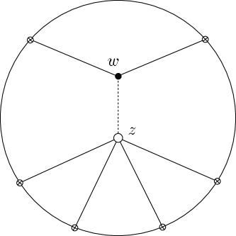
Figure 1: A tree process with a D-instanton vertex at $z$ and a classical supergravity vertex at $w$. Solid lines denote bulk-to-boundary propagators, the dotted one a bulk-to-bulk propagator.

When considering the non minimal correlation functions we are interested in there are other effects which need to be taken into account. These correspond to processes in which one of the vertices is a multiparticle vertex induced by a D-instanton and there are additional tree level perturbative interactions in the bulk. An example of such a diagram is illustrated in figure 1. Here the point $z$ represents a D-instanton induced vertex. The amplitude involves another interaction vertex, at the point $w$, which is a standard supergravity interaction. The dashed line corresponds to a bulk-to-bulk propagator for one of the fields entering the D-instanton induced interaction. In view of the above discussion this can be either one of the fields in ${\cal R}^{4}$, $\Lambda^{16}$ etc. or a dilaton or graviton in the induced $\hat{\tau}^{k}{\cal R}^{4}$, $({\rm tr}h^{k})^{l}{\cal R}^{4}$, $\hat{\tau}^{k}\Lambda^{16}$, $({\rm tr}h^{k})^{l}\Lambda^{16}$, …interactions. Moreover the intermediate state can also be any Kaluza–Klein excited state allowed by the symmetries. The plain lines in the figure represent usual bulk-to-boundary propagators. We will discuss various similar processes in the following sections. It is important to notice that all the tree level AdS diagrams with fixed external states are of the same order when all the appropriate factors of the coupling associated with vertices and bulk propagators are included . The contribution of amplitudes of this type is needed in particular to match the Yang–Mills result in the case of the correlation function (74).

The general analysis of such processes would be very complicated. We will focus on those relevant for the interpretation of the Yang–Mills calculation of some simple non-minimal correlators. In these cases very specific diagrams are selected by the conditions imposed by the $SU(4)$ symmetry and by the $U(1)$ symmetry of classical supergravity.

In the next subsection we present the Yang–Mills calculation of (74) in the one-instanton sector, then in the following subsection we describe the supergravity calculation and show how the agreement with field theory is recovered. In section 6 we discuss another example of non minimal correlation function with insertions of higher dimensional operators corresponding to Kaluza–Klein excited states on the gravity side. Section 7 contains an overview of other correlation functions which also involve the various processes described here.

5.1 One-instanton contribution to ${\hat{\Lambda}^{16}{\cal Q}_{2}^{2}}$ in ${\cal N}=4$ SYM

The operator insertions in (74) contain 24 fermion modes at lowest order in the coupling, thus ${\bar{\nu}}\nu$ pairs must be included beyond the 16 exact superconformal modes. Each $\hat{\Lambda}^{A}_{\alpha}$ operator soaks up one superconformal mode and does not depend on the $\nu$ and ${\bar{\nu}}$ modes, so that the latter only enter into the ${\cal Q}_{2}$ insertions. A non-vanishing result in the semiclassical limit is obtained by replacing each ${\cal Q}_{2}$ by its expression in terms of $(\bar{\nu}\nu)_{\bf 10}$ bilinears given in appendix D. This contribution contains four $(\bar{\nu}\nu)_{\bf 10}$ pairs, which according to the general analysis of section 3.2 bring four powers of $g_{{}_{\rm YM}}$. The other relevant contributions are obtained by contracting pairs of $\varphi$ fields in the two ${\cal Q}_{2}$’s with a propagator: one can either contract two $\varphi$’s and saturate the remaining two with ${\bar{\nu}}$ and $\nu$ modes or contract both pairs of scalar fields.

Taking into account the powers of $g_{{}_{\rm YM}}$ associated with the propagators discussed in section 3.3 and those associated with ${\bar{\nu}}\nu$ insertions, (42) and (43), we see that all three types of contributions occur at the same leading non-vanishing order in the coupling and must be included in the semiclassical approximation. Notice that the only fields whose fluctuations must be considered are the scalars. We will denote the above three types of processes as follows

$$\hat{G}_{\hat{\Lambda}^{16}{\cal Q}_{2}^{2}}=\hat{G}_{\hat{\Lambda}^{16}{\cal Q}_{2}^{2}}^{\rm(a)}+\hat{G}_{\hat{\Lambda}^{16}{\cal Q}_{2}^{2}}^{\rm(b)}+\hat{G}_{\hat{\Lambda}^{16}{\cal Q}_{2}^{2}}^{\rm(c)}$$ (76)

They are represented diagrammatically in figure 2.

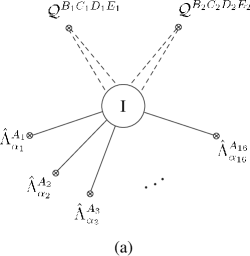
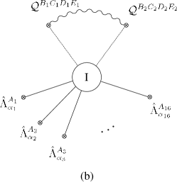
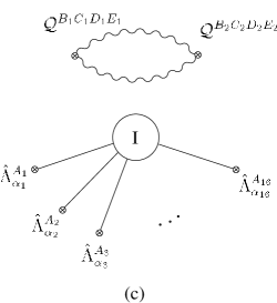
Figure 2: The three types of contributions to the correlation function $\hat{G}_{\hat{\Lambda}^{16}{\cal Q}_{2}^{2}}$: wiggly lines denote scalar propagators, a plain line corresponds to the insertion of a superconformal mode, a $\bar{\nu}\nu$ pair is indicated by a dashed line when in the 10 and by a dotted line when in the 6.

We first consider the ‘purely instantonic’ process depicted in figure 2(a). In the semiclassical approximation we must evaluate 

$$\hat{G}_{\hat{\Lambda}^{16}{\cal Q}_{2}^{2}}^{\rm(a)} \!=\! \int d\mu_{\rm phys}\,{\rm e}^{-S_{4F}}\left[\hat{\Lambda}^{A_{1}}_{{\alpha}_{1}}(x_{1})\ldots\hat{\Lambda}^{A_{16}}_{{\alpha}_{16}}(x_{16}){\cal Q}_{2}^{[B_{1}C_{1}][D_{1}E_{1}]}(y_{1}){\cal Q}_{2}^{[B_{2}C_{2}][D_{2}E_{2}]}(y_{2})\right]$$ (77)

$$\!=\! \frac{1}{g_{{}_{\rm YM}}^{36}}\int d\mu_{\rm phys}\,{\rm e}^{-S_{4F}}\,\left[\prod_{i=1}^{16}\frac{\rho^{4}\zeta^{A_{i}}_{{\alpha}_{i}}}{[(x_{i}-x_{0})^{2}+\rho^{2}]^{4}}\right.$$

$$\left.\prod_{j=1}^{2}\frac{\displaystyle({\bar{\nu}}^{u(B_{j}}\nu^{D_{j})}_{u})({\bar{\nu}}^{v(C_{j}}\nu^{E_{j}}_{v})-({\bar{\nu}}^{u(B_{j}}\nu^{E_{j})}_{u})({\bar{\nu}}^{v(C_{j}}\nu^{D_{j})}_{v})}{[(y_{j}-x_{0})^{2}+\rho^{2}]^{2}}\right]\,,$$

where we have substituted the classical expressions for the operators $\hat{\Lambda}$ and ${\cal Q}_{2}$ which are given by (276) and (280), respectively. The combinatorics necessary to evaluate the $8(N-2)$ fermionic integrations over $\bar{\nu}^{A}_{u}$ and $\nu^{A}_{u}$ is performed with the aid of the generating function (36) by rewriting the above expression as

$$\hat{G}_{\hat{\Lambda}^{16}{\cal Q}_{2}^{2}}^{\rm(a)} \!=\! \frac{g_{{}_{\rm YM}}^{-28}{\rm e}^{2\pi i\tau}}{(N-1)!(N-2)!}\int d\rho\,d^{4}x_{0}\,d^{5}\Omega\prod_{A=1}^{4}d^{2}\eta^{A}\,d^{2}{\bar{\xi}}^{A}\,\rho^{4N-7}\int_{0}^{\infty}dr\,r^{4N-3}{\rm e}^{-2\rho^{2}r^{2}}$$

$$\left\{\prod_{i=1}^{16}\frac{\rho^{4}}{[(x_{i}-x_{0})^{2}+\rho^{2}]^{4}}\zeta^{A_{i}}_{{\alpha}_{i}}\prod_{j=1}^{2}\frac{1}{[(y_{j}-x_{0})^{2}+\rho^{2}]^{2}}\right.$$

$$\left.\left.\left[\frac{\delta^{8}{\cal Z}(\vartheta,{\bar{\vartheta}};\Omega,r)}{\delta\vartheta_{u_{1}(B_{1}}\delta{\bar{\vartheta}}_{C_{1})}^{u_{1}}\delta\vartheta_{u_{2}(D_{1}}\delta{\bar{\vartheta}}_{E_{1})}^{u_{2}}\delta\vartheta_{u_{3}(B_{2}}\delta{\bar{\vartheta}}_{C_{2})}^{u_{3}}\delta\vartheta_{u_{4}(D_{2}}\delta{\bar{\vartheta}}_{E_{4})}^{u_{4}}}-(D_{j}\leftrightarrow E_{j})\right]\right|_{\vartheta={\bar{\vartheta}}=0}\right\}\,,$$

where the measure has been explicitly written in terms of integrations over the collective coordinates.

The $(\bar{\nu}\nu)_{\bf 10}$ insertions are replaced by $\vartheta$ derivatives of ${\cal Z}(\vartheta,{\bar{\vartheta}};\Omega,r)$. The resulting integration over angular variables, $\Omega$, selects the combination of ${\bar{\nu}}$ and $\nu$ modes forming a singlet of $SU(4)$. After performing the $\vartheta$ derivatives and symmetrising the indices as in (5.1) we obtain angular integrals which can be performed using

$$\int\!d^{5}\Omega\,\Omega^{A_{1}B_{1}}\Omega^{A_{2}B_{2}}\Omega^{A_{3}B_{3}}\Omega^{A_{4}B_{4}}=\frac{1}{2^{6}}\!\int_{\sum_{e=1}^{6}\!\Omega_{e}^{2}}\prod_{e=1}^{6}d\Omega_{e}\,\Omega_{a}\Omega_{b}\Omega_{c}\Omega_{d}{\bar{\Sigma}}^{A_{1}B_{1}}_{a}{\bar{\Sigma}}^{A_{2}B_{2}}_{b}{\bar{\Sigma}}^{A_{3}B_{3}}_{c}{\bar{\Sigma}}^{A_{4}B_{4}}_{d}$$

$$\rule{0.0pt}{16.0pt}=\frac{1}{2^{6}}\left(\delta_{ab}\delta_{cd}+\delta_{ac}\delta_{bd}+\delta_{ad}\delta_{bc}\right){\bar{\Sigma}}^{A_{1}B_{1}}_{a}{\bar{\Sigma}}^{A_{2}B_{2}}_{b}{\bar{\Sigma}}^{A_{3}B_{3}}_{c}{\bar{\Sigma}}^{A_{4}B_{4}}_{d}$$

$$\rule{0.0pt}{20.0pt}=\frac{1}{2^{4}}\left(\varepsilon^{A_{1}B_{1}A_{2}B_{2}}\varepsilon^{A_{3}B_{3}A_{4}B_{4}}+\varepsilon^{A_{1}B_{1}A_{3}B_{3}}\varepsilon^{A_{2}B_{2}A_{4}B_{4}}+\varepsilon^{A_{1}B_{1}A_{4}B_{4}}\varepsilon^{A_{2}B_{2}A_{3}B_{3}}\right)\,.$$ (79)

The $SU(4)$ singlet tensor resulting from the five-sphere integration is

$$t^{B_{1}C_{1}D_{1}E_{1}B_{2}C_{2}D_{2}E_{2}}=-\varepsilon^{B_{1}E_{1}C_{2}E_{2}}\>\varepsilon^{C_{1}D_{1}B_{2}D_{2}}+\varepsilon^{B_{1}E_{1}C_{2}D_{2}}\>\varepsilon^{C_{1}D_{1}B_{2}E_{2}}$$

$$+\varepsilon^{B_{1}E_{1}B_{2}E_{2}}\>\varepsilon^{C_{1}D_{1}C_{2}D_{2}}-\varepsilon^{B_{1}E_{1}B_{2}D_{2}}\>\varepsilon^{C_{1}D_{1}C_{2}E_{2}}+\varepsilon^{B_{1}D_{1}C_{2}E_{2}}\>\varepsilon^{C_{1}E_{1}B_{2}D_{2}}$$

$$-\varepsilon^{B_{1}D_{1}C_{2}D_{2}}\>\varepsilon^{C_{1}E_{1}B_{2}E_{2}}-\varepsilon^{B_{1}D_{1}B_{2}E_{2}}\>\varepsilon^{C_{1}E_{1}C_{2}D_{2}}+\varepsilon^{B_{1}D_{1}B_{2}D_{2}}\>\varepsilon^{C_{1}E_{1}C_{2}E_{2}}$$

$$+2\left(\varepsilon^{B_{1}E_{1}D_{2}E_{2}}\>\varepsilon^{C_{1}D_{1}C_{2}B_{2}}+\varepsilon^{B_{1}E_{1}C_{2}B_{2}}\>\varepsilon^{C_{1}D_{1}D_{2}E_{2}}+\varepsilon^{B_{1}D_{1}D_{2}E_{2}}\>\varepsilon^{C_{1}E_{1}B_{2}C_{2}}\right.$$

$$+\varepsilon^{B_{1}D_{1}B_{2}C_{2}}\>\varepsilon^{C_{1}E_{1}D_{2}E_{2}}+\varepsilon^{B_{1}C_{1}C_{2}E_{2}}\>\varepsilon^{D_{1}E_{1}B_{2}D_{2}}+\varepsilon^{B_{1}C_{1}D_{2}C_{2}}\>\varepsilon^{D_{1}E_{1}B_{2}E_{2}}$$

$$\left.+\varepsilon^{B_{1}C_{1}E_{2}B_{2}}\>\varepsilon^{D_{1}E_{1}C_{2}D_{2}}+\varepsilon^{B_{1}C_{1}B_{2}D_{2}}\>\varepsilon^{D_{1}E_{1}C_{2}E_{2}}\right)+4\left(\varepsilon^{B_{1}C_{1}D_{2}E_{2}}\>\varepsilon^{D_{1}E_{1}B_{2}C_{2}}\right.$$

$$\left.+\varepsilon^{B_{1}C_{1}B_{2}C_{2}}\>\varepsilon^{D_{1}E_{1}D_{2}E_{2}}\right)\,.$$

The expression for $\hat{G}_{\hat{\Lambda}^{16}{\cal Q}_{2}^{2}}^{\rm(a)}$ becomes

$$\hat{G}_{\hat{\Lambda}^{16}{\cal Q}_{2}^{2}}^{\rm(a)} \!=\! t^{B_{1}C_{1}D_{1}E_{1}B_{2}C_{2}D_{2}E_{2}}g_{{}_{\rm YM}}^{-24}{\rm e}^{2\pi i\tau}\int d\rho\,d^{4}x_{0}\prod_{A=1}^{4}d^{2}\eta^{A}\,d^{2}{\bar{\xi}}^{A}\,\rho^{4N-7}$$ (80)

$$\left[\prod_{i=1}^{16}\frac{\rho^{4}}{[(x_{i}-x_{0})^{2}+\rho^{2}]^{4}}\zeta^{A_{i}}_{{\alpha}_{i}}\prod_{j=1}^{2}\frac{1}{[(y_{j}-x_{0})^{2}+\rho^{2}]^{2}}\right]$$

$$\frac{(N^{2}-5N+6)}{(N-1)!(N-2)!}\int_{0}^{\infty}dr\,r^{4N-7}{\rm e}^{-2\rho^{2}r^{2}}\,,$$

where the numerator $(N^{2}-5N+6)=(N-2)^{2}-(N-2)$ in the last line is the result of the colour contractions in the $(\bar{\nu}\nu)_{\bf 10}$ insertions. All factors of $N$ are now isolated by performing the $r$ integral, giving

$$\frac{N^{2}-5N+6}{(N-1)!(N-2)!}\int_{0}^{\infty}dr\,r^{4N-7}{\rm e}^{-2\rho^{2}r^{2}}=\frac{(N^{2}-5N+6)\Gamma(2N-3)}{(N-1)!(N-2)!}2^{2-2N}\rho^{6-4N}\,.$$ (81)

Including all the numerical coefficients the final result is

$$\hat{G}_{\hat{\Lambda}^{16}{\cal Q}_{2}^{2}}^{\rm(a)} = C_{\rm a}(N)\,t^{B_{1}C_{1}D_{1}E_{1}B_{2}C_{2}D_{2}E_{2}}\frac{2^{39}3^{19}{\rm e}^{2\pi i\tau}}{\pi^{35/2}g_{{}_{\rm YM}}^{24}}\int\frac{d\rho\,d^{4}x_{0}}{\rho^{5}}\prod_{A=1}^{4}d^{2}\eta^{A}\,d^{2}{\bar{\xi}}^{A}$$ (82)

$$\left[\prod_{i=1}^{16}\frac{\rho^{4}}{[(x_{i}-x_{0})^{2}+\rho^{2}]^{4}}\zeta^{A_{i}}_{{\alpha}_{i}}\prod_{j=1}^{2}\frac{\rho^{2}}{[(y_{j}-x_{0})^{2}+\rho^{2}]^{2}}\right]\,,$$

where

$$C_{\rm a}(N)=N^{1/2}\left(1-\frac{25}{8N}-\frac{47}{128N^{2}}+O(1/N^{3})\right)\,.$$ (83)

We will discuss the interpretation of this result in the next subsection, let us only note here that the integration over $(\Omega,r)$ determines the $SU(4)$ tensorial structure and produces the powers of $N$ that lead to the above overall $N$-dependence as well as the factors of $\rho$ that reconstruct the functions $K_{2}(y_{j};x_{0},\rho)$ for each ${\cal Q}_{2}$ insertion, see (66).

The $\hat{G}^{\rm(b)}_{\hat{\Lambda}^{16}{\cal Q}_{2}^{2}}$ term in (76) corresponds to contributions in which one pair of scalar fields is contracted via a propagator, see figure 2(b),

$$\hat{G}^{\rm(b)}_{\hat{\Lambda}^{16}{\cal Q}_{2}^{2}} \!=\! \langle{\rm Tr}\!\left(F_{m_{1}n_{1}}\sigma^{m_{1}n_{1}}_{{\alpha}_{1}}{}^{\beta_{1}}\lambda^{A_{1}}_{\beta_{1}}\right)\!(x_{1})\ldots{\rm Tr}\!\left(F_{m_{16}n_{16}}\sigma^{m_{16}n_{16}}_{{\alpha}_{16}}{}^{\beta_{16}}\lambda^{A_{16}}_{\beta_{16}}\right)\!(x_{16})$$ (84)

$$\left[2{\rm Tr}\left(\varphi^{B_{1}C_{1}}\varphi^{D_{1}E_{1}}\right)(y_{1})\,2{\rm Tr}\left(\varphi^{B_{2}C_{2}}\varphi^{D_{2}E_{2}}\right)(y_{2})\raisebox{-10.0pt}{ \rule{0.4pt}{4.0pt}\rule{108.12054pt}{0.4pt}\rule{0.4pt}{4.0pt}}\hskip 81.09052pt+\cdots\right]\rangle\,,$$

where the ellipsis refers to 35 other terms. The 36 terms in (84) come from the expansion of the product of the two ${\cal Q}$ insertions using (57) which gives nine terms and from the application of Wick’s theorem which gives four contractions for each term. In this expression the sixteen factors of $\hat{\Lambda}$ soak up the superconformal modes as in the case of $\hat{G}^{\rm(a)}_{\hat{\Lambda}^{16}{\cal Q}_{2}^{2}}$ and the remaining $\varphi$ fields which are not contracted into a propagator should be saturated by $\bar{\nu}$ and $\nu$ modes.

The calculation of the contribution of a contraction between a pair of scalar fields in two ${\cal Q}$ operators is reported in appendix E. All the contractions in (84) give rise to the same spatial structure and combining them together determines the $SU(4)$ tensorial form of $\hat{G}^{\rm(b)}_{\hat{\Lambda}^{16}{\cal Q}_{2}^{2}}$. In computing a single contraction only the terms in the first and fourth lines in the expression for the propagator (53) contribute because the other terms produce traces over single $\varphi$ fields which vanish since the fields are in $SU(N)$. This simplification would not occur in the case of a similar contraction between operators formed by the product of three or more elementary fields as we will see in the example discussed in the next section.

Substituting the result (284) in the appendix into (84) and replacing the remaining fields with their expressions in the instanton background gives

$$\hat{G}^{\rm(b)}_{\hat{\Lambda}^{16}{\cal Q}_{2}^{2}} \!=\! g_{{}_{\rm YM}}^{-34}\varepsilon^{B_{1}C_{1}B_{2}C_{2}}\int d\mu_{\rm phys}{\rm e}^{-S_{4F}}\,\left[\prod_{i=1}^{16}\frac{\rho^{4}}{[(x_{i}-x_{0})^{2}+\rho^{2}]^{4}}\zeta^{A_{i}}_{{\alpha}_{i}}\right]$$ (85)

$$\left\{\frac{1}{32\pi^{2}(y_{1}-y_{2})^{2}[(y_{1}-x_{0})^{2}+\rho^{2}][(y_{2}-x_{0})^{2}+\rho^{2}]}\left[(\bar{\nu}^{[D_{1}}\nu^{D_{2}]})(\bar{\nu}^{[E_{2}}\nu^{E_{1}]})\right.\right.$$

$$\rule{0.0pt}{18.0pt}\!-(\bar{\nu}^{[D_{1}}\nu^{E_{2}]})(\bar{\nu}^{[D_{2}}\nu^{E_{1}]})-(\bar{\nu}^{[D_{1}}\nu^{E_{1}]})(\bar{\nu}^{[D_{2}}\nu^{E_{2}]})+(\bar{\nu}^{(D_{1}}\nu^{D_{2})})(\bar{\nu}^{(E_{1}}\nu^{E_{2})})$$

$$\rule{0.0pt}{18.0pt}\!\left.\left.-(\bar{\nu}^{(D_{1}}\nu^{E_{2})})(\bar{\nu}^{(D_{2}}\nu^{E_{1})})\right]+\cdots\right\}\,,$$

where the dots stand for the contributions of the other contractions. Notice in particular that combining the two types of terms induced by the scalar propagator in (283)-(284) leads to the cancellation of a contact contribution, i.e. a term non singular in the limit $y_{2}\to y_{1}$, so that only one spatial structure appears in (85). To evaluate this expression we follow the same steps as in the case of $\hat{G}^{\rm(a)}_{\hat{\Lambda}^{16}{\cal Q}_{2}^{2}}$, we first rewrite the ${\bar{\nu}}\nu$ bilinears as derivatives of the density ${\cal Z}(\vartheta,{\bar{\vartheta}};\Omega,r)$ and then compute the resulting six-dimensional integral over $(\Omega,r)$. In particular the angular integrals over $\Omega$ select an $SU(4)$ singlet. This is a common feature of all the non-minimal correlation functions, the ${\bar{\nu}}\nu$ pairs in the operator insertions must always be combined to form a singlet of the $SU(4)$ R-symmetry group. This implies that the last two terms in (85) vanish when integrated over the five-sphere because the product ${\bf 10}\otimes{\bf 10}$ does not contain the singlet. After rewriting (85) in terms of the generating function ${\cal Z}(\vartheta,{\bar{\vartheta}};\Omega,r)$ and performing the $\vartheta$ derivatives, all the angular integrals are computed using

$$\int d^{5}\Omega\,\Omega^{AB}\Omega^{BC}=\frac{1}{2^{2}}\,\varepsilon^{ABCD}\,.$$ (86)

We then have to combine the terms in (85) corresponding to all the possible Wick contractions. In conclusion we find

$$\hat{G}^{\rm(b)}_{\hat{\Lambda}^{16}{\cal Q}_{2}^{2}}\! =\! g_{{}_{\rm YM}}^{-24}{\rm e}^{2\pi i\tau}t^{B_{1}C_{1}D_{1}E_{1}B_{2}C_{2}D_{2}E_{2}}\int d\rho\,d^{4}x_{0}\prod_{A=1}^{4}d^{2}\eta^{A}\,d^{2}{\bar{\xi}}^{A}$$ (87)

$$\rho^{4N-7}\left[\prod_{i=1}^{16}\frac{\rho^{4}}{[(x_{i}-x_{0})^{2}+\rho^{2}]^{4}}\zeta^{A_{i}}_{{\alpha}_{i}}\right]\frac{1}{(y_{1}-y_{2})^{2}}\left[\prod_{j=1}^{2}\frac{1}{[(y_{j}-x_{0})^{2}+\rho^{2}]}\right]$$

$$\frac{(N^{2}-5N+6)}{(N-1)!(N-2)!}\int_{0}^{\infty}dr\,r^{4N-5}{\rm e}^{-2\rho^{2}r^{2}}\,,$$

where $t^{B_{1}C_{1}D_{1}E_{1}B_{2}C_{2}D_{2}E_{2}}$ is the same tensor defined in (5.1) which appeared in $\hat{G}^{\rm(a)}_{\hat{\Lambda}^{16}{\cal Q}_{2}^{2}}$. Note, however, that this same $SU(4)$ tensorial structure is obtained here in a completely different way. In $\hat{G}^{\rm(a)}_{\hat{\Lambda}^{16}{\cal Q}_{2}^{2}}$ it was the result of five dimensional integrals of the form (79) whereas here it is obtained combining the 36 terms associated with all the possible contractions with the appropriate weights. The $N$-dependence is determined by the integral over the radial variable $r$. Performing this integral and reintroducing all the numerical coefficients we finally obtain

$$\hat{G}_{\hat{\Lambda}^{16}{\cal Q}_{2}^{2}}^{\rm(b)} \!=\! C_{\rm b}(N)t^{B_{1}C_{1}D_{1}E_{1}B_{2}C_{2}D_{2}E_{2}}\frac{2^{46}3^{16}{\rm e}^{2\pi i\tau}}{\pi^{35/2}g_{{}_{\rm YM}}^{24}}\int\frac{d\rho\,d^{4}x_{0}}{\rho^{5}}\prod_{A=1}^{4}d^{2}\eta^{A}\,d^{2}{\bar{\xi}}^{A}$$ (88)

$$\left[\prod_{i=1}^{16}\frac{\rho^{4}}{[(x_{i}-x_{0})^{2}+\rho^{2}]^{4}}\zeta^{A_{i}}_{{\alpha}_{i}}\right]\frac{1}{(y_{1}-y_{2})^{2}}\left[\prod_{j=1}^{2}\frac{\rho}{[(y_{j}-x_{0})^{2}+\rho^{2}]}\right]\,,$$

where

$$C_{\rm b}(N)=N^{3/2}\left(1-\frac{37}{8N}+\frac{553}{128N^{2}}+O(1/N^{3})\right)\,.$$ (89)

Notice that the leading term in $\hat{G}_{\hat{\Lambda}^{16}{\cal Q}_{2}^{2}}^{\rm(b)}$ is of order $N^{3/2}$. Such a contribution could not have an AdS counterpart, since D-instanton effects appear in the type IIB effective action at order $({\alpha^{\prime}})^{-1}$, i.e. $N^{1/2}$. As we will show the leading term in (88) is cancelled by an equal and opposite term from the other contribution to $\hat{G}_{\hat{\Lambda}^{16}{\cal Q}_{2}^{2}}$ which we will now discuss.

The third type of instanton correction to the correlation function $\langle\hat{\Lambda}^{16}{\cal Q}^{2}\rangle$ is obtained by contracting both pairs of scalars in the two ${\cal Q}_{2}$ insertions by propagators, see figure 2(c),

$$\hat{G}_{\hat{\Lambda}^{16}{\cal Q}_{2}^{2}}^{\rm(c)} \!=\! \langle{\rm Tr}\!\left(F_{m_{1}n_{1}}\sigma^{m_{1}n_{1}}_{{\alpha}_{1}}{}^{\beta_{1}}\lambda^{A_{1}}_{\beta_{1}}\right)\!(x_{1})\ldots{\rm Tr}\!\left(F_{m_{16}n_{16}}\sigma^{m_{16}n_{16}}_{{\alpha}_{16}}{}^{\beta_{16}}\lambda^{A_{16}}_{\beta_{16}}\right)\!(x_{16})$$ (90)

$$\left[4{\rm Tr}\left(\varphi^{B_{1}C_{1}}\varphi^{D_{1}E_{1}}\right)(y_{1})\,{\rm Tr}\left(\varphi^{B_{2}C_{2}}\varphi^{D_{2}E_{2}}\right)(y_{2})\raisebox{-15.0pt}{ \rule{0.4pt}{10.0pt}\rule{130.88284pt}{0.4pt}\rule{0.4pt}{10.0pt}}\raisebox{-10.0pt}{ \rule{0.4pt}{4.0pt}\rule{73.97733pt}{0.4pt}\rule{0.4pt}{4.0pt}}\hskip 79.6678pt+\cdots\right]\rangle\,,$$

where again the ellipsis is for 17 terms corresponding to the other Wick contractions. In (90) all the scalars are contracted, the $\hat{\Lambda}$ insertions saturate the sixteen superconformal modes and no $\nu$ and ${\bar{\nu}}$ modes are involved. The double contraction is significantly more complicated to evaluate than the single contraction entering $\hat{G}_{\hat{\Lambda}^{16}{\cal Q}_{2}^{2}}^{\rm(b)}$ since now all the terms in the propagator (53) contribute. The result is given in (287) in appendix E. Since there is no dependence on the additional fermion modes ${\bar{\nu}}$ and $\nu$, substituting into (90) leads to the same type of integrals encountered in the computation of minimal correlation functions. Collecting terms of the same order in $N$ from the double contraction we have

$$\hat{G}_{\hat{\Lambda}^{16}{\cal Q}_{2}^{2}}^{\rm(c)} \!=\! \frac{\varepsilon^{B_{1}C_{1}D_{2}E_{2}}\varepsilon^{D_{1}E_{1}B_{2}C_{2}}\,{\rm e}^{2\pi i\tau}}{g_{{}_{\rm YM}}^{24}(N-1)!(N-2)!}\int d\rho\,d^{4}x_{0}\,d^{5}\Omega\prod_{A=1}^{4}d^{2}\eta^{A}\,d^{2}{\bar{\xi}}^{A}\,\rho^{4N-7}$$ (91)

$$\int_{0}^{\infty}dr\,r^{4N-3}{\rm e}^{-2\rho^{2}r^{2}}\left[\prod_{i=1}^{16}\frac{\rho^{4}}{[(x_{i}-x_{0})^{2}+\rho^{2}]^{4}}\zeta^{A_{i}}_{{\alpha}_{i}}\right]\left\{\rule{0.0pt}{20.0pt}\frac{(N^{2}-1)}{(y_{1}-y_{2})^{4}}\right.$$

$$-N\frac{1}{(y_{1}-y_{2})^{2}}\prod_{j=1}^{2}\frac{\rho}{[(y_{j}-x_{0})^{2}+\rho^{2}]}+\left[5\prod_{j=1}^{2}\frac{\rho^{2}}{[(y_{j}-x_{0})^{2}+\rho^{2}]^{2}}\right.$$

$$\left.+\frac{1}{(y_{1}-y_{2})^{2}}\prod_{j=1}^{2}\frac{\rho}{[(y_{j}-x_{0})^{2}+\rho^{2}]}\right]+\frac{1}{N}\left[2\prod_{j=1}^{2}\frac{\rho^{2}}{[(y_{j}-x_{0})^{2}+\rho^{2}]^{2}}\right.$$

$$\left.\left.-{1\over 2}\frac{1}{(y_{1}-y_{2})^{2}}\prod_{j=1}^{2}\frac{\rho}{[(y_{j}-x_{0})^{2}+\rho^{2}]}\right]\right\}+\cdots\,.$$

In (91) we have not included terms of order $1/N^{2}$ from (287) since they give rise to subleading effects beyond the order we are interested in for the comparison with string theory.

Combining the contributions of the various contractions and computing the integrals over $(\Omega,r)$ gives

$$\!\!\hat{G}_{\hat{\Lambda}^{16}{\cal Q}_{2}^{2}}^{\rm(c)}=\hat{G}_{\hat{\Lambda}^{16}{\cal Q}_{2}^{2}}^{\rm(c1)}+\hat{G}_{\hat{\Lambda}^{16}{\cal Q}_{2}^{2}}^{\rm(c2)}+\hat{G}_{\hat{\Lambda}^{16}{\cal Q}_{2}^{2}}^{\rm(c3)}$$

$$\!\!=t^{B_{1}C_{1}D_{1}E_{1}B_{2}C_{2}D_{2}E_{2}}\frac{2^{46}3^{16}{\rm e}^{2\pi i\tau}}{\pi^{35/2}g_{{}_{\rm YM}}^{24}}\int\frac{d\rho\,d^{4}x_{0}}{\rho^{5}}\prod_{A=1}^{4}d^{2}\eta^{A}\,d^{2}{\bar{\xi}}^{A}\left[\prod_{i=1}^{16}\frac{\rho^{4}}{[(x_{i}-x_{0})^{2}+\rho^{2}]^{4}}\zeta^{A_{i}}_{{\alpha}_{i}}\right]$$

$$\!\!\left\{C_{\rm c1}(N)\frac{1}{(y_{1}-y_{2})^{4}}+C_{\rm c2}(N)\left[\frac{1}{(y_{1}-y_{2})^{2}}\prod_{j=1}^{2}\frac{\rho}{[(y_{j}-x_{0})^{2}+\rho^{2}]}\right]\right.$$

$$+\left.C_{\rm c3}(N)\left[\prod_{j=1}^{2}\frac{\rho^{2}}{[(y_{j}-x_{0})^{2}+\rho^{2}]^{2}}\right]\right\}\,,$$ (92)

where the tensor $t^{B_{1}C_{1}D_{1}E_{1}B_{2}C_{2}D_{2}E_{2}}$ is the same which appears in the previous contributions and we have reinstated all the numerical coefficients. There three different spatial structures that appear in (92) and the $N$-dependence is encoded in the coefficients $C_{\rm c1}(N)$, $C_{\rm c2}(N)$ and $C_{\rm c3}(N)$ for which we obtain

$$C_{\rm c1}(N)=\frac{1}{4}(N^{2}-1)N^{1/2}\left(1-\frac{5}{8N}-\frac{23}{128N^{2}}+O(1/N^{3})\right)$$ (93)

$$C_{\rm c2}(N)=N^{3/2}\left(-1+\frac{1}{6N}-\frac{139}{288N^{2}}+O(1/N^{3})\right)$$ (94)

$$C_{\rm c3}(N)=N^{1/2}\left(1+\frac{5}{4N}+\frac{101}{48N^{2}}+O(1/N^{3})\right)\,.$$ (95)

In (92) we have separated the contribution $\hat{G}_{\Lambda^{16}{\cal Q}_{2}^{2}}^{\rm(c1)}$ which starts at order $N^{5/2}$ which, as will be discussed in the next subsection, corresponds to a disconnected AdS diagram. The other two terms, $\hat{G}_{\Lambda^{16}{\cal Q}_{2}^{2}}^{\rm(c2)}$ and $\hat{G}_{\Lambda^{16}{\cal Q}_{2}^{2}}^{\rm(c3)}$, must be combined respectively with $\hat{G}_{\Lambda^{16}{\cal Q}_{2}^{2}}^{\rm(b)}$ and $\hat{G}_{\Lambda^{16}{\cal Q}_{2}^{2}}^{\rm(a)}$.

In conclusion we get

$$\hat{G}_{\hat{\Lambda}^{16}{\cal Q}_{2}^{2}}=\hat{G}_{\hat{\Lambda}^{16}{\cal Q}_{2}^{2}}^{\rm(disc)}+\hat{G}_{\hat{\Lambda}^{16}{\cal Q}_{2}^{2}}^{\rm(conn)}\,,$$ (96)

where

$$\hat{G}_{\hat{\Lambda}^{16}{\cal Q}_{2}^{2}}^{\rm(disc)}=\hat{G}_{\Lambda^{16}{\cal Q}_{2}^{2}}^{\rm(c1)}$$ (97)

and

$$\hat{G}_{\hat{\Lambda}^{16}{\cal Q}_{2}^{2}}^{\rm(conn)} \!=\! t^{B_{1}C_{1}D_{1}E_{1}B_{2}C_{2}D_{2}E_{2}}\frac{2^{46}3^{16}{\rm e}^{2\pi i\tau}}{\pi^{35/2}g_{{}_{\rm YM}}^{24}}\int\frac{d\rho\,d^{4}x_{0}}{\rho^{5}}\prod_{A=1}^{4}d^{2}\eta^{A}\,d^{2}{\bar{\xi}}^{A}$$ (98)

$$\left[\prod_{i=1}^{16}\frac{\rho^{4}}{[(x_{i}-x_{0})^{2}+\rho^{2}]^{4}}\zeta^{A_{i}}_{{\alpha}_{i}}\right]\left\{C_{1}(N)\frac{1}{(y_{1}-y_{2})^{2}}\left[\prod_{j=1}^{2}\frac{\rho}{[(y_{j}-x_{0})^{2}+\rho^{2}]}\right]\right.$$

$$+\left.C_{2}(N)\left[\prod_{j=1}^{2}\frac{\rho^{2}}{[(y_{j}-x_{0})^{2}+\rho^{2}]^{2}}\right]\right\}$$

$$C_{1}(N)=-\frac{107}{24}N^{1\over 2}+\frac{4421}{1152}N^{-{1\over 2}}+O\left(N^{-\frac{3}{2}}\right)$$ (99)

$$C_{2}(N)=\frac{155}{128}N^{1\over 2}+\frac{605}{1024}N^{-{1\over 2}}+O\left(N^{-\frac{3}{2}}\right)\,.$$ (100)

As already anticipated in the introductory discussion we obtain, apart from the disconnected term $\hat{G}_{\hat{\Lambda}^{16}{\cal Q}_{2}^{2}}^{\rm(disc)}$, two different spatial structures contributing to the correlation function $\hat{G}_{\hat{\Lambda}^{16}{\cal Q}_{2}^{2}}$ and both have a leading term of order $N^{1/2}$, whereas one would have naively expected a result of order $N^{-1/2}$. In the next subsection we compare the result with the supergravity calculation of the dual amplitude and we discuss the interpretation of this result.

5.2 The ${\hat{\Lambda}^{16}{\cal Q}_{2}^{2}}$ correlator in supergravity

The AdS computation of the correlation function (74) at leading non-vanishing order in the coupling constant involves various different processes of the type described in the introduction to this section. Let us first list all the relevant contributions at each order in $N$, then we will proceed with the description of the individual diagrams. The AdS amplitudes we have to consider are represented in figure 3.

         

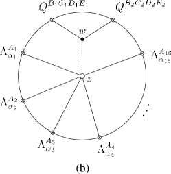
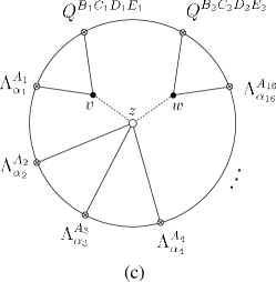
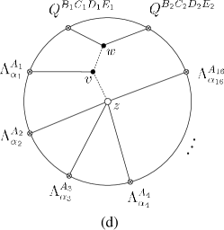
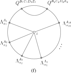
Figure 3: AdS diagrams contributing to the correlation function $G_{\Lambda^{16}Q_{2}^{2}}$.

Diagram (a) corresponds to a structure which appears at order $N^{1/2}$ as well as $N^{-1/2}$. The $N^{1/2}$ contribution comes from a $\Lambda^{16}$ vertex at order ${\alpha^{\prime}}^{-1}$ with two $Q_{2}$ insertions coming from the expansion of $\sqrt{-g}$. Here and in the following we are using the symbol $Q_{\ell}$ as a shortcut to denote the bulk field corresponding to the operator ${\cal Q}_{\ell}$ in the boundary field theory, i.e. a linear combination of the trace part of the metric and the RR four-form with indices on the five-sphere. The order $N^{-1/2}$ contribution with the structure in (a) comes from the ${\cal R}^{2}\Lambda^{16}$ vertex at order ${\alpha^{\prime}}$ as well as from subleading corrections to the leading $N^{1/2}$ term. Diagram (b) represents an amplitude starting at order $N^{1/2}$ and resulting from the insertion of a $Q_{\ell}$ coming from the expansion of $\sqrt{-g}$ in the $\Lambda^{16}$ vertex. The perturbative vertex at the point $w$ is a $Q_{\ell}Q_{2}Q_{2}$ cubic interaction, where $\ell$ takes any value allowed by the $SU(4)$ selection rules. The amplitudes in (c), (d) and (e) all have leading terms of order $N^{1/2}$, plus $1/N$ corrections, which correspond to a $\Lambda^{16}$ interaction with additional perturbative vertices. We will see that in the case (c) the dashed lines correspond to dilatini in the second Kaluza–Klein excited mode, which transform in the 60 of $SU(4)$. In the case (d) there are different possibilities for the bulk-to-bulk propagators between the points $v$, $w$ and $z$ and we will analyse the details below. Finally we will see that a potential contribution with the structure in (e) actually vanishes. Diagram (f) is a disconnected amplitude. Its leading term is of order $N^{5/2}$, resulting from a factor of $N^{2}$ carried by the factorised two-point function and a factor of $N^{1/2}$ associated with the D-instanton vertex in $z$. This contribution can be matched separately with the one of order $N^{5/2}$ in the Yang–Mills calculation. In all the other cases it will be crucial for our comparison with the field theory calculation that all the interactions involved in these processes are either of the extremal or of the next-to-extremal type [34, 35, 36, 37, 38, 12]. In analysing the various contributions we will make use of the techniques and results of these papers, the reader is referred, for instance, to the appendix of [12] for a detailed discussion of the technical aspects.

To compare the results with field theory we need to normalise the AdS amplitudes appropriately. With our definitions of the Yang–Mills operators the normalisation of the external states in the supergravity processes does not involve any powers of $N$ or $g_{\rm s}$. The exact numerical normalisations will not be important in our subsequent analysis but they can be fixed by the matching of two-point functions as, for instance, in [27]. We will use the standard notation $K_{\Delta}(z;x)=K_{\Delta}(z_{m},z_{0};x_{m})$ to denote the bulk-to-boundary propagator from the point $(z_{m},z_{0})$ in $AdS_{5}$ to the boundary point $x_{m}$ for a supergravity field corresponding to a scalar operator of dimension $\Delta$ [2, 3, 39]. A superscript $F$ is used to distinguish the propagators for fermionic operators.

Let us first consider the disconnected diagram 3(f). This amplitude simply gives

$$G_{\Lambda^{16}Q^{2}}^{\rm(f)}=\langle Q(y_{1})Q(y_{2})\rangle\langle\Lambda(x_{1})\dots\Lambda(x_{16})\rangle\,,$$ (101)

where the factorised two-point function is given by the free field theory result and the remaining sixteen-point function coincides with the minimal correlation function of [5, 6]. Thus we get

$$G_{\Lambda^{16}Q^{2}}^{\rm(f)}=\frac{c_{\rm f}(\tau,\bar{\tau},N)}{(y_{1}-y_{2})^{4}}\int\frac{d^{5}z}{z_{0}^{5}}\prod_{i=1}^{16}K_{7/2}^{F}(z;x_{i})\,,$$ (102)

with

$$c_{\rm f}(\tau,\bar{\tau},N)=c_{\rm f}N^{5/2}g_{\rm s}^{-12}{\rm e}^{2\pi i\tau}\,,$$ (103)

where $c_{\rm f}$ is a non-zero numerical constant which can be determined from the known normalisations of the two-point function and the minimal $\langle\Lambda^{16}\rangle$ correlator. As already observed the overall power of $N$ comes from a factor of $N^{2}$ associated with the two-point function times a $N^{1/2}$ from the D-instanton correction to the minimal sixteen-point function. The bulk-to-boundary propagator for the dilatini, $K^{F}_{7/2}$, corresponding to the fermionic operator $\hat{\Lambda}$ of dimension $7/2$ was given in [40, 5] and reads

$$K^{F}_{7/2}(z_{m},z_{0};x_{m}) = K_{4}(z_{m},z_{0};x_{m})\frac{1}{\sqrt{z_{0}}}\left(z_{0}\gamma_{\hat{5}}+(z-x)^{m}\gamma_{\hat{m}}\right)$$ (104)

$$= \frac{z_{0}^{4}}{[(z-x)^{2}+z_{0}^{2}]^{4}}\frac{1}{\sqrt{z_{0}}}\left(z_{0}\gamma_{\hat{5}}+(z-x)^{m}\gamma_{\hat{m}}\right)\,,$$

so that the spatial dependence in (102) agrees with the field theory result. With our normalisations the two point-function is independent of $g_{\rm s}$ and the minimal sixteen-point function is proportional to $g_{\rm s}^{-12}$. This contribution reproduces the leading $N^{5/2}$ disconnected term $\hat{G}^{\rm(c1)}_{\hat{\Lambda}^{16}{\cal Q}^{2}}$ of (92)-(93) in the Yang–Mills calculation. Notice that in the Yang–Mills calculation the disconnected contribution with the spatial structure matching the supergravity result (102) arises with a coefficient

$$C_{\rm c1}(N)=\left(N^{2}-1\right)N^{1/2}\left(1+O(1/N)\right)\,.$$ (105)

The above calculation reproduces the leading order term in (105). The full two-point function in supergravity is, however, expected to reproduce exactly the field theory result, which means that it actually should produce a factor of $(N-1)^{2}$ which matches that in (105). Moreover the $1/N$ corrections in the Yang–Mills result can also be explained on the gravity side: they are produced by amplitudes involving higher ${\alpha^{\prime}}$ vertices that contribute to the minimal correlator of 16 dilatini via the mechanism described at the end of section 3.

The AdS diagram in figure 3(a) is a contact diagram and it is straightforward to evaluate since it has the same structure as those contributing to the minimal correlation functions. As noted above a contribution with this structure is obtained from the $({\rm tr}\,h)^{2}\Lambda^{16}$ coupling produced by expanding the $\sqrt{-g}$ factor in the $\Lambda^{16}$ vertex in the effective action at order ${\alpha^{\prime}}^{-1}$ and then simply replacing all the fields with the appropriate bulk-to-boundary propagators. Moreover a contribution with exactly the same form comes from the ${\cal R}^{2}\Lambda^{16}$ vertex at order ${\alpha^{\prime}}$. The total contribution of diagram (a) is

$$G_{\Lambda^{16}Q^{2}}^{\rm(a)}=c_{\rm a}(\tau,\bar{\tau},N)\int\frac{d^{5}z}{z_{0}^{5}}\,\prod_{i=1}^{16}K^{F}_{7/2}(z;x_{i})\prod_{j=1}^{2}K_{2}(z;y_{j})\,,$$ (106)

In (106) the coefficient $c_{\rm a}(\tau,\bar{\tau},N)$ is the sum of a term of order $N^{1/2}$ and one of order $N^{-1/2}$. It encodes the information about the D-instanton induced part of the modular forms appearing in the relevant vertices. The explicit form of the two terms in $c_{\rm a}(\tau,\bar{\tau},N)$ can be read from the general formula (24). For the comparison with the result of the super Yang–Mills calculation we are interested in the dependence on $N$ and on the coupling. For this purpose notice in particular that the leading D-instanton term in all the modular forms $f_{l}^{(0,0)}(\tau,\bar{\tau})$ has no powers of $\tau_{2}=g_{\rm s}^{-1}$. For the coefficient in (106) we get

$$c_{\rm a}(\tau,\bar{\tau},N)=c_{\rm a1}N^{1/2}g_{\rm s}^{-12}{\rm e}^{2\pi i\tau}+c_{\rm a2}N^{-1/2}g_{\rm s}^{-12}{\rm e}^{2\pi i\tau}\,,$$ (107)

where $c_{\rm a1}$ and $c_{\rm a2}$ are numerical coefficients independent of $N$ and $g_{\rm s}$ and the powers of the coupling come from the expansion (2) of the modular functions $f^{(12,-12)}_{1}(\tau,\bar{\tau})$ and $f^{(12,-12)}_{2}(\tau,\bar{\tau})$ appearing in the $\Lambda^{16}$ and ${\cal R}^{2}\Lambda^{16}$ vertices respectively.

Diagram 3(b) is an exchange amplitude and we must analyse the contribution of all the possible intermediate states. The vertex in $z$ is a $({\rm tr}\,h)\Lambda^{16}$ coupling of order ${\alpha^{\prime}}^{-1}$, where the ${\rm tr}\,h$ insertion is obtained again by expanding $\sqrt{-g}$. Notice that a similar diagram involving a $\tau\,\Lambda^{16}$ coupling is not present because a cubic coupling of a dilaton in any Kaluza–Klein mode with two $Q$’s is forbidden by the $U(1)$ symmetry of classical supergravity. Hence the dashed line can correspond only to a $Q$ in any Kaluza–Klein level allowed by the $SU(4)$ selection rules. The amplitude in figure 3 (b) is thus

$$G_{\Lambda^{16}Q^{2}}^{\rm(b)}=c_{\rm b}(\tau,\bar{\tau},N)\int\frac{d^{5}z}{z_{0}^{5}}\frac{d^{5}w}{w_{0}^{5}}\,\prod_{i=1}^{16}K^{F}_{7/2}(z;x_{i})G_{\ell}(z,w)\prod_{j=1}^{2}K_{2}(w;y_{j})\,,$$ (108)

where $G_{\ell}(z,w)$ is a bulk-to-bulk propagator for the field corresponding to the chiral primary ${\cal Q}_{\ell}$. The $SU(4)$ symmetry only allows $\ell=2,4$. In the case $\ell=2$ the vertex in $w$ is next to extremal and the $w$ integration can be done using the formulae derived in [41] for the general scalar exchange. An exchange diagram with two bulk integrals as in (108) can be reduced to a sum of contact contributions. In this case there is only one term in the sum which at leading order takes the form

$$\frac{c_{\rm b1}(\tau,\bar{\tau},N)}{(y_{1}-y_{2})^{2}}\int\frac{d^{5}z}{z_{0}^{5}}\,\prod_{i=1}^{16}K^{F}_{7/2}(z;x_{i})\prod_{j=1}^{2}K_{1}(z;y_{j})\,,$$ (109)

with

$$c_{\rm b1}(\tau,\bar{\tau},N)=c_{\rm b1}N^{1/2}g_{\rm s}^{-12}{\rm e}^{2\pi i\tau}\,.$$ (110)

In the case $\ell=4$ the coupling in $w$ is extremal and the resulting amplitude reduces to a contact contribution. The tree diagram in figure 3(b) should be thought of as representing the ten dimensional amplitude. Then the integration over the five-sphere selects the intermediate states allowed by the $SO(6)$ symmetry, which are the scalars with $\ell=2,4$ in the present case. One can then simplify the integral over the $AdS_{5}$ point $w$ by integrating by parts the derivatives appearing in the cubic coupling. In the case of the extremal vertex the derivatives taken to act on the $G_{\ell}(z,w)$ bulk-to-bulk propagator reconstruct the wave operator, so that the only contribution that is left is a contact diagram. Hence the corresponding amplitude becomes

$$c_{\rm b2}(\tau,\bar{\tau},N)\int\frac{d^{5}z}{z_{0}^{5}}\,\prod_{i=1}^{16}K^{F}_{7/2}(z;x_{i})\prod_{j=1}^{2}K_{2}(z;y_{j})\,,$$ (111)

where

$$c_{\rm b2}(\tau,\bar{\tau},N)=c_{\rm b2}N^{1/2}g_{\rm s}^{-12}{\rm e}^{2\pi i\tau}\,.$$ (112)

Notice that, unlike in the cases encountered in evaluating four-point functions, in this case the new contact term obtained in $AdS_{5}$ is not extremal or next-to-extremal.

In diagram 3(c) the two cubic vertices in $v$ and $w$ involve a dilatino and a $Q_{2}$ combination, thus the dashed lines correspond to dilatini in an allowed Kaluza–Klein mode. The only intermediate states permitted by the $SU(4)$ symmetry are in the representation $[1,2,0]$, i.e. in the 60. The vertex in $z$ is hence the usual $\Lambda^{16}$ interaction where two of the fields are taken in their second Kaluza–Klein excited level. As a consequence the vertices in $v$ and $w$ are extremal. More precisely they are superconformal descendants of a standard extremal coupling of chiral primaries. Then the same mechanism discussed above reduces the amplitude to

$$G_{\Lambda^{16}Q^{2}}^{\rm(c)}=c_{\rm c}(\tau,\bar{\tau},N)\int\frac{d^{5}z}{z_{0}^{5}}\,\prod_{i=1}^{16}K^{F}_{7/2}(z;x_{i})\prod_{j=1}^{2}K_{2}(z;y_{j})\,,$$ (113)

where

$$c_{\rm c}(\tau,\bar{\tau},N)=c_{\rm c}N^{1/2}g_{\rm s}^{-12}{\rm e}^{2\pi i\tau}\,.$$ (114)

Here again the factors of $N$ and $g_{\rm s}$ are those associated with the $\Lambda^{16}$ vertex.

The amplitude in diagram (d) is the most complicated that we have to consider. Denoting by $\phi$ and $\phi^{\prime}$ the two bulk fields exchanged between $v$ and $w$ and between $v$ and $z$ respectively we obtain

$$G_{\Lambda^{16}Q^{2}}^{\rm(d)}=c_{\rm d}(\tau,\bar{\tau},N)\int\frac{d^{5}z}{z_{0}^{5}}\frac{d^{5}v}{(v_{0})^{5}}\frac{d^{5}w}{(w_{0})^{5}}\,\prod_{i=1}^{16}K^{F}_{7/2}(z;x_{i})\,G_{\phi^{\prime}}(z,v)\,G_{\phi}(v,w)\prod_{j=1}^{2}K_{2}(w;y_{j})\,.$$ (115)

The vertex in $z$ is $\Lambda^{16}$ so that $\phi^{\prime}$ is a dilatino or one of its Kaluza–Klein excited states. Starting form the vertex in $w$ the allowed $SU(4)$ representations for the field $\phi$ are $[0,2,0]$, $[0,4,0]$, $[2,0,2]$ and $[0,0,0]$, i.e. ${\bf 20^{\prime}}$, ${\bf 105}$, ${\bf 84}$ and ${\bf 1}$. The first two correspond to $Q_{2}$ and $Q_{4}$ respectively, the third one is a scalar coming from internal components of the metric and the last one is a graviton. When $\phi$ is in the $[0,2,0]$ $\phi^{\prime}$ can only be in the $[1,2,0]$, i.e. it is a dilatino in the second Kaluza–Klein excited level. In this case the vertex at $w$ is next-to-extremal and the one at $v$ is a descendant of an extremal vertex. The integration in $w$ can be carried out using the formulae in [41] and from the resulting extremal vertex in $v$ we get a contribution of the form is

$$G_{\Lambda^{16}Q^{2}}^{\rm(d1)}=\frac{c_{\rm d1}(\tau,\bar{\tau},N)}{(y_{1}-y_{2})^{2}}\int\frac{d^{5}z}{z_{0}^{5}}\,\prod_{i=1}^{16}K^{F}_{7/2}(z;x_{i})\,\prod_{j=1}^{2}K_{1}(z;y_{j})\,.$$ (116)

with

$$c_{\rm d1}(\tau,\bar{\tau},N)=c_{\rm d1}N^{1/2}g_{\rm s}^{-12}{\rm e}^{2\pi i\tau}\,.$$ (117)

When $\phi$ is in the $[0,4,0]$ the coupling in $w$ is extremal and the integral is finite so that the amplitude vanishes. The same happens in the case of $\phi=h_{({\alpha}\beta)}$ in the $[2,0,2]$ since this is a superconformal descendant of $Q_{4}$. The case of the graviton exchange is more involved and we will not discuss it in detail. In this case the only allowed state for the dilatino $\phi^{\prime}$ is the Kaluza–Klein ground state. The integrals in $w$ and $v$ can be sequentially performed using the techniques of [41, 33] reducing the amplitude to a sum of terms of the same form as those in (106) and (109).

The amplitude corresponding to diagram 3(e) involves a $\Lambda^{16}$ vertex in $z$. The bulk lines from $z$ to $v$ and from $v$ to $w$ are dilatini in allowed Kaluza–Klein levels. The $SU(4)$ selection rules imply in particular that the second one is in the $[1,2,0]$. This means that the coupling in $w$ is extremal and thus the whole contribution vanishes because the integral is finite.

There are, in principle, other possible contributions to the exchange diagrams considered above. These involve other D-instanton induced vertices at order ${\alpha^{\prime}}^{-1}$. For instance, there is a vertex of the form [10]

$$f_{1}^{(11,-11)}(\tau,\bar{\tau})\Lambda^{15}\gamma^{\mu}\psi^{*}_{\mu}\,.$$ (118)

This could contribute to diagrams (d) and (e) in figure 3. However, the possibility of such processes is ruled out by $U(1)$ conservation at one of the cubic interactions involved. For instance, in the case of diagram (d) if the vertex in $z$ were (118) then the bulk state exchanged between $v$ and $w$ would be $U(1)$ charged because the dilatino and the gravitino have different $U(1)$ charges. But then the coupling in $w$ would not be allowed because the $Q$’s are not charged. An analogous argument can be applied to the case of diagram (e). In this case if the state exchanged between $z$ and $v$ is a gravitino then $U(1)$ conservation at $v$ implies that the bulk line between $v$ and $w$ is also a gravitino, but then the coupling in $w$ would violate the $U(1)$ selection rule. Similar arguments can be applied to rule out the possibility of contributions from amplitudes involving the vertices $G\Lambda^{14}$ and $\psi^{2}\Lambda^{14}$.

In conclusion, combining the various AdS amplitudes we can recapitulate the result as follows. There is an order $N^{5/2}$ disconnected amplitude of the form of (102). This corresponds to the Yang–Mills contribution of (92)-(93). The other terms are of order $N^{1/2}$ and $N^{-1/2}$. These are of two different types

$$a\int\frac{d^{5}z}{z_{0}^{5}}\,\prod_{i=1}^{16}K^{F}_{7/2}(z;x_{i})\prod_{j=1}^{2}K_{2}(z;y_{j})+\frac{b}{(y_{1}-y_{2})^{2}}\int\frac{d^{5}z}{z_{0}^{5}}\,\prod_{i=1}^{16}K^{F}_{7/2}(z;x_{i})\prod_{j=1}^{2}K_{1}(z;y_{j})\,,$$ (119)

where the coefficients $a$ and $b$ contain terms of order $N^{1/2}$ and $N^{-1/2}$,

$$a=a_{1}g_{\rm s}^{-12}N^{1/2}+a_{2}g_{\rm s}^{-12}N^{-1/2}$$ (120)

$$b=b_{1}g_{\rm s}^{-12}N^{1/2}+b_{2}g_{\rm s}^{-12}N^{-1/2}\,.$$ (121)

The dependence on the parameters, $g_{{}_{\rm YM}}^{2}=4\pi g_{\rm s}$ and $N$, as well as the spatial dependence in this result are exactly those found in the Yang–Mills calculation of the previous subsection, (96)-(100). In particular, the agreement of the spatial structure is highly non-trivial. It is achieved after combining many types of terms in a calculation which is significantly more complicated than the one required in the case of minimal correlation functions. It would be satisfying to be able to make a detailed correspondence between the coefficients in the Yang–Mills instanton calculation and those of supergravity D-instanton contributions to the $\Lambda^{16}Q^{2}$ interaction. However, there are ambiguities that our analysis has not resolved. We can identify the amplitudes contributing to the leading terms of order $N^{1/2}$ in (121). The contact amplitude — the first term in (119) — receives contributions from the terms (a), (b2) and (c) in the previous analysis,

$$a_{1}=c_{\rm a}+c_{\rm b2}+c_{\rm c}\,.$$ (122)

Similarly the second term in (119) gets contributions from the processes (b1) and (d1), so that

$$b_{1}=c_{\rm b1}+c_{\rm d1}\,.$$ (123)

These coefficients are, in principle, computable although the calculation is rather subtle because it involves the tree level processes described in this section. The situation is even more complicated for the subleading terms of order $N^{-1/2}$ in (121). On the Yang–Mills side we have a precise expression for the term of order $N^{-1/2}$, which is the first $1/N$ correction to the leading one-instanton contribution to the $\hat{\Lambda}^{16}\,{\cal Q}^{2}$ correlation function (as always, in semi-classical approximation). This comes from expanding the instanton measure and taking into account the subleading contributions in the diagrams coming both from the scalar contractions and from the $({\bar{\nu}}\nu)$ insertions. On the string side it should come from terms of order ${\alpha^{\prime}}$. For this specific correlation function the relevant coupling at this order should be ${\alpha^{\prime}}\,\sqrt{-g}\,{\rm e}^{\phi/2}\,\Lambda^{16}\,{\cal R}^{2}$. Naively, our calculation leads to a prediction for the coefficient of this conjectured interaction in (2). However, another order $\alpha^{\prime}$ effect is almost certainly present, which complicates matters. This arises from the potential presence of a ${\alpha^{\prime}}\,\sqrt{-g}\,{\rm e}^{9\phi/2}\,\Lambda^{16}\,F_{5}^{4}$ term. Since $F_{5}$ has a nonzero background value this interaction makes a contribution to the $\hat{\Lambda}^{16}$ correlation function that is suppressed by a power of $1/N$ relative to the leading instanton term. This is the effect that produces the $1/N$ corrections to minimal correlation functions that were mentioned in section 3. However, the same interaction also generates a new $\Lambda^{16}\,h$ vertex which can be joined by a $\langle hh\rangle$ propagator to a classical $h^{3}$ vertex. This generates a tree diagram that contributes to the $\hat{\Lambda}^{16}\,{\cal Q}^{2}$ correlation function at order $N^{-1/2}$, which is the same order as the ${\alpha^{\prime}}\,\sqrt{-g}\,{\rm e}^{\phi/2}\,\Lambda^{16}\,{\cal R}^{2}$. In general for all the processes considered in this section which involved a $\Lambda^{16}$ vertex generating a contribution of order $N^{1/2}$ there is a corresponding amplitude of order $N^{-1/2}$ in which the D-instanton induced vertex is $\Lambda^{16}\,F_{5}^{4}$, and the five-form factors are replaced by their background value. This explains the fact that the contribution we found at order $N^{-1/2}$ is not purely a contact amplitude as would be the case if it came entirely from the ${\alpha^{\prime}}\,\sqrt{-g}\,{\rm e}^{\phi/2}\,\Lambda^{16}\,{\cal R}^{2}$ vertex. In conclusion, although the Yang–Mills calculation shows the presence of various order ${\alpha^{\prime}}$ interactions, our calculation does not pin down their relative coefficients.

6 Non-minimal correlation functions in the instanton background: Kaluza–Klein excited states

In this section we illustrate the general features of correlations functions involving operators corresponding to Kaluza-Klein excited modes in supergravity. As in the previous section we focus on a specific example in order to highlight the general properties of these processes. The new aspect that emerges is the rôle played by $\bar{\nu}\nu$ bilinears in the 6 of $SU(4)$.

From the string theory point of view there is little distinction between amplitudes in which the boundary fields are in their Kaluza–Klein ground states or in excited states. This means that for any of the minimal processes that contribute at order $N^{1/2}$ there should be similar contributions when the external legs are in excited Kaluza–Klein states. The only additional selection rule is imposed by the $SU(4)$ symmetry. On the Yang–Mills side the operators corresponding to Kaluza–Klein excitations are higher dimensional with respect to the ones associated with supergravity states. This means that they soak up more fermion modes and thus their correlation functions are non-minimal and involve the presence of $\nu$ and $\bar{\nu}$ fermionic variables.

We consider here the example of the $\Lambda^{16}$ interaction at order ${\alpha^{\prime}}^{-1}$. Instead of taking all the $\Lambda$’s in their Kaluza–Klein ground state, i.e. in the ${\bf 4}$ of $SU(4)$, we might consider the process in which two of them are in the first excited state, i.e. in the ${\bf 20^{*}}$. This is a combination allowed by $SU(4)$ selection rules. We analyse the Yang–Mills calculation first and then compare the results with the AdS calculation.

6.1 One-instanton contribution in ${\cal N}=4$ SYM

The process we are interested in corresponds to the correlation function

$$\hat{G}_{\hat{\Lambda}^{14}_{\bf 4}\hat{\Lambda}^{2}_{\bf 20^{*}}}(x_{1},\ldots,x_{14},y_{1},y_{2})=\langle\hat{\Lambda}_{\bf 4}(x_{1})\ldots\hat{\Lambda}_{\bf 4}(x_{14})\hat{\Lambda}_{\bf 20^{*}}(y_{1})\hat{\Lambda}_{\bf 20^{*}}(y_{2})\rangle\,.$$ (124)

Here $\hat{\Lambda}_{\bf 4}$ is the fermionic operator dual to the type IIB dilatino already considered in the previous section and $\hat{\Lambda}_{\bf 20^{*}}$ denotes the operator of (4.2), which corresponds to the first Kaluza–Klein mode of the dilatino. The correlation function (124) involves 20 fermionic modes. Analogously to the case described in the previous section there are two types of contributions to this correlation function at leading order in the coupling in the one-instanton sector. The first is obtained by the standard semiclassical approximation replacing the operators with their expressions in the instanton background. This means that each operator insertion soaks up one superconformal mode and in addition the two $\hat{\Lambda}_{\bf 20^{*}}$ insertions involve a $(\bar{\nu}\nu)_{\bf 6}$ bilinear each. The second type of contribution corresponds to a leading order quantum correction to the semiclassical approximation and arises from contracting two scalars between the operators $\hat{\Lambda}_{\bf 20^{*}}$. Thus we have

$$\hat{G}_{\hat{\Lambda}^{14}_{\bf 4}\hat{\Lambda}^{2}_{\bf 20^{*}}}=\hat{G}_{\hat{\Lambda}^{14}_{\bf 4}\hat{\Lambda}^{2}_{\bf 20^{*}}}^{({\rm a})}+\hat{G}_{\hat{\Lambda}^{14}_{\bf 4}\hat{\Lambda}^{2}_{\bf 20^{*}}}^{({\rm b})}$$ (125)

and the two types of contributions are represented in figure 4.

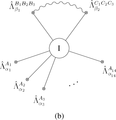
Figure 4: The two types of contributions to the correlation function $\hat{G}_{\hat{\Lambda}^{14}_{\bf 4}\hat{\Lambda}^{2}_{\bf 20^{*}}}$. As before, plain lines correspond to superconformal modes, wiggly lines are scalar propagators and dotted lines are used to indicate the insertion of $\bar{\nu}\nu$ pairs in the 6 of $SU(4)$.

The first term in (125) is given by

$${\hat{G}}_{\hat{\Lambda}^{14}_{\bf 4}\hat{\Lambda}^{2}_{\bf 20^{*}}}^{({\rm a})} \!=\! \int d\mu_{\rm phys}\,{\rm e}^{-S_{4F}}\left[\hat{\Lambda}^{A_{1}}_{{\alpha}_{1}}(x_{1})\ldots\hat{\Lambda}^{A_{14}}_{{\alpha}_{14}}(x_{14})\hat{\Lambda}^{B_{1}B_{2}B_{3}}_{\beta_{1}}(y_{1})\hat{\Lambda}^{C_{1}C_{2}C_{3}}_{\beta_{2}}(y_{2})\right]$$ (126)

$$\!=\! \frac{1}{g_{{}_{\rm YM}}^{34}N}\int d\mu_{\rm phys}\,{\rm e}^{-S_{4F}}\,\prod_{i=1}^{14}\frac{\rho^{4}\zeta^{A_{i}}_{{\alpha}_{i}}}{[(x_{i}-x_{0})^{2}+\rho^{2}]^{4}}\prod_{j=1}^{2}\frac{\rho^{4}}{[(y_{j}-x_{0})^{2}+\rho^{2}]^{5}}$$

$$\left[\left(\zeta^{B_{2}}_{\beta_{1}}\bar{\nu}^{[B_{1}}\nu^{B_{3}]}+\zeta^{B_{3}}_{\beta_{1}}\bar{\nu}^{[B_{1}}\nu^{B_{2}]}\right)\left(\zeta^{C_{2}}_{\beta_{2}}\bar{\nu}^{[C_{1}}\nu^{C_{3}]}+\zeta^{C_{3}}_{\beta_{2}}\bar{\nu}^{[C_{1}}\nu^{C_{2}]}\right)\right]\,,$$

where we have substituted the classical expressions (276) and (282) for the operators $\Lambda_{\bf 4}$ and $\Lambda_{\bf 20^{*}}$ respectively and we have omitted numerical coefficients which will be reinstated in the final expression. Notice in particular the powers of $g_{{}_{\rm YM}}$ and $N$ in the prefactor which are dictated by the normalisation of the operators. According to the general rule (54) for the normalisation of Yang–Mills operators each $\hat{\Lambda}_{\bf 4}$ brings a factor of $g_{{}_{\rm YM}}^{-2}$ and each $\hat{\Lambda}_{\bf 20^{*}}$ a factor of $g_{{}_{\rm YM}}^{-3}N^{-1/2}$. In terms of the generating function (36) the above expression is rewritten as

$$\hat{G}_{\hat{\Lambda}^{14}_{\bf 4}\hat{\Lambda}^{2}_{\bf 20^{*}}}^{({\rm a})}=\frac{1}{g_{{}_{\rm YM}}^{34}N}\frac{g_{{}_{\rm YM}}^{8}{\rm e}^{2\pi i\tau}}{(N-1)!(N-2)!}\int d\rho\,d^{4}x_{0}\,d^{5}\Omega\prod_{A=1}^{4}d^{2}\eta^{A}\,d^{2}{\bar{\xi}}^{A}\,\rho^{4N-7}$$

$$\int_{0}^{\infty}dr\,r^{4N-3}{\rm e}^{-2\rho^{2}r^{2}}\,\prod_{i=1}^{14}\frac{\rho^{4}}{[(x_{i}-x_{0})^{2}+\rho^{2}]^{4}}\zeta^{A_{i}}_{{\alpha}_{i}}\prod_{j=1}^{2}\frac{\rho^{4}}{[(y_{j}-x_{0})^{2}+\rho^{2}]^{5}}$$

$$\left\{\left(\zeta^{B_{2}}_{\beta_{1}}\zeta^{C_{2}}_{\beta_{2}}\left.\left[\frac{\delta^{4}{\cal Z}(\vartheta,{\bar{\vartheta}};\Omega,r)}{\delta\vartheta_{u_{1}[B_{1}}\delta{\bar{\vartheta}}_{B_{3}]}^{u_{1}}\delta\vartheta_{u_{2}[C_{1}}\delta{\bar{\vartheta}}_{C_{3}]}^{u_{2}}}\right]\right|_{\vartheta={\bar{\vartheta}}=0}+(B_{2}\leftrightarrow B_{3})\right)+(C_{2}\leftrightarrow C_{3})\right\}\,,$$ (127)

where the integrations over the collective coordinates have been indicated explicitly. After performing the derivatives we can compute the angular integrals using (86). As in the cases described in the previous section there is a factorisation of the angular integrals, which implies that the indices carried by the $\nu$ and $\bar{\nu}$ modes are combined separately in a $SU(4)$ singlet. Proceeding as in section 5.1 we then carry out the integration over the radial variable $r$ to extract the dependence on $g_{{}_{\rm YM}}$ and $N$ and get

$$\hat{G}_{\hat{\Lambda}^{14}_{\bf 4}\hat{\Lambda}^{2}_{\bf 20^{*}}}^{({\rm a})} \!=\! C_{\rm a}(N)\,\frac{{\rm e}^{2\pi i\tau}}{g_{{}_{\rm YM}}^{24}}\int\frac{d\rho\,d^{4}x_{0}}{\rho^{5}}\prod_{A=1}^{4}d^{2}\eta^{A}\,d^{2}{\bar{\xi}}^{A}\,\prod_{i=1}^{14}\frac{\rho^{4}}{[(x_{i}-x_{0})^{2}+\rho^{2}]^{4}}\zeta^{A_{i}}_{{\alpha}_{i}}$$ (128)

$$\left(\varepsilon^{B_{1}B_{3}C_{1}C_{3}}\frac{\rho^{5}}{[(y_{1}-x_{0})^{2}+\rho^{2}]^{5}}\zeta^{B_{2}}_{\beta_{1}}\frac{\rho^{5}}{[(y_{2}-x_{0})^{2}+\rho^{2}]^{5}}\zeta^{C_{2}}_{\beta_{2}}+\cdots\right)\,,$$

where the $\cdots$ refers to symmetrisation in the ($B_{2}$,$B_{3}$) and ($C_{2}$,$C_{3}$) pairs of indices. The $N$-dependence is enclosed in the prefactor

$$C_{\rm a}(N)=\frac{2^{44}3^{18}}{\pi^{35/2}}N^{1/2}\left(1-\frac{25}{8N}+O(1/N^{2})\right)\,.$$ (129)

Integration over the fermion zero modes $\eta$ and $\bar{\xi}$ produces the same completely antisymmetric tensor $t_{(16)}$ that enters in the calculation of the correlator of sixteen $\hat{\Lambda}$’s in the 4 [5]. In the next subsection we will see how this result agrees with the AdS calculation. In particular the powers of $g_{{}_{\rm YM}}$ and $N$ are the same as in the minimal correlation function of sixteen $\hat{\Lambda}_{\bf 4}$: the factors of $g_{{}_{\rm YM}}\sqrt{N}$ associated with each $(\bar{\nu}\nu)_{\bf 6}$ insertion are compensated by the normalisation of the operators. From the supergravity point of view (128) will be interpreted as a sum of terms involving the product of fourteen bulk-to-boundary propagators $K^{F}_{7/2}$ for the $\hat{\Lambda}_{\bf 4}$ insertions and two propagators $K^{F}_{9/2}$ for the $\hat{\Lambda}_{\bf 20^{*}}$ insertions. In each term the $SU(4)$ indices are combined in a singlet tensor of the form $\varepsilon_{(4)}t_{(16)}$.

The second type of contribution to the correlation function we are considering, $\hat{G}_{\hat{\Lambda}^{14}_{\bf 4}\hat{\Lambda}^{2}_{\bf 20^{*}}}^{({\rm b})}$, involves a scalar propagator, see figure 4(b). It comes from the contraction

$$\hat{G}_{\hat{\Lambda}^{14}_{\bf 4}\hat{\Lambda}^{2}_{\bf 20^{*}}}^{({\rm b})} \!= \langle{\rm Tr}\!\left(F_{{\alpha}_{1}}{}^{\beta_{1}}\lambda^{A_{1}}_{\gamma_{1}}\right)\!(x_{1})\ldots{\rm Tr}\!\left(F_{{\alpha}_{14}}{}^{\gamma_{14}}\lambda^{A_{14}}_{\beta_{14}}\right)\!(x_{14})$$ (130)

$${\rm Tr}\left(\left\{F_{\beta_{1}}{}^{\delta_{1}},\lambda^{B_{2}}_{\delta_{1}}\right\}\varphi^{B_{1}B_{3}}\right)(y_{1})\,{\rm Tr}\left(\left\{F_{\beta_{2}}{}^{\delta_{2}},\lambda^{C_{2}}_{\delta_{2}}\right\}\varphi^{C_{1}C_{3}}\right)(y_{2})\rangle\raisebox{-10.0pt}{ \rule{0.4pt}{4.0pt}\rule{140.27187pt}{0.4pt}\rule{0.4pt}{4.0pt}}\hskip 56.9055pt+\cdots\,,$$

where we are using the notation $F_{\alpha}{}^{\gamma}=F_{mn}\sigma_{\>{\alpha}}^{mn\,\gamma}$ and the ellipsis refers again to terms obtained by symmetrisation in ($B_{2}$,$B_{3}$) and ($C_{2}$,$C_{3}$). Notice that as in the case examined in the previous section there is no similar contribution involving contractions of the $\lambda$’s or the $F$’s. For this reason in evaluating $\hat{G}_{\hat{\Lambda}^{14}_{\bf 4}\hat{\Lambda}^{2}_{\bf 20^{*}}}^{({\rm b})}$ we do not need to consider the term cubic in the fermions in the operators $\hat{\Lambda}_{\bf 20^{*}}$. Using the form of the scalar propagator given in section 3.3 to expand (130) we get a rather complicated expression that is given in (288) of appendix E. In particular, unlike in the case of the $\hat{G}_{\hat{\Lambda}^{16}{\cal Q}^{2}}$ correlation function, here the $1/N$ and $1/N^{2}$ terms in the propagator (53) do contribute because the operator $\hat{\Lambda}_{\bf 20^{*}}$ is cubic in the elementary fields. However, all the contributions obtained from the expansion of (288) are subleading in the large $N$ limit with respect to (128)-(129), which had an additional factor of $N$ coming from the colour contractions in the $(\bar{\nu}\nu)_{\bf 6}$ bilinears to compensate the $1/N$ from the normalisation of the operators. The dependence on $N$ in (288) arises entirely from the instanton measure and the normalisation of the Klauza–Klein operators and thus the dominant terms are of order $N^{-1/2}$. We only consider these leading order contributions in the following discussion. Expanding (288) we obtain two types of terms with different spatial dependence. The structure of the two contributions is

$$\hat{G}_{\hat{\Lambda}^{14}_{\bf 4}\hat{\Lambda}^{2}_{\bf 20^{*}}}^{({\rm b})} \!=\! C_{\rm b}(N)\,\frac{{\rm e}^{2\pi i\tau}}{g_{{}_{\rm YM}}^{24}}\int\frac{d\rho\,d^{4}x_{0}}{\rho^{5}}\prod_{A=1}^{4}d^{2}\eta^{A}\,d^{2}{\bar{\xi}}^{A}\,\prod_{i=1}^{14}\frac{\rho^{4}}{[(x_{i}-x_{0})^{2}+\rho^{2}]^{4}}\zeta^{A_{i}}_{{\alpha}_{i}}$$ (131)

$$\left[\varepsilon^{B_{1}B_{3}C_{1}C_{3}}\left(c_{\rm b1}\,\frac{\rho^{5}}{[(y_{1}-x_{0})^{2}+\rho^{2}]^{5}}\zeta^{B_{2}}_{\beta_{1}}\frac{\rho^{5}}{[(y_{2}-x_{0})^{2}+\rho^{2}]^{5}}\zeta^{C_{2}}_{\beta_{2}}\right.\right.$$

$$\left.\left.+\,c_{\rm b2}\,\frac{1}{(y_{1}-y_{2})^{2}}\frac{\rho^{4}}{[(y_{1}-x_{0})^{2}+\rho^{2}]^{4}}\zeta^{B_{2}}_{\beta_{1}}\frac{\rho^{4}}{[(y_{2}-x_{0})^{2}+\rho^{2}]^{4}}\zeta^{C_{2}}_{\beta_{2}}\right)+\cdots\right]\,,$$

where, as in the previous expressions, the ellipsis stands for symmetrisation in the pairs ($B_{2}$,$B_{3}$) and ($C_{2}$,$C_{3}$). We find that the coefficients $c_{\rm b1}$ and $c_{\rm b2}$ in (131) are both non-vanishing. This is a puzzling result. The first term has the structure of a contact amplitude. It contributes a $1/N$ correction to (128) which, as we shall discuss in the next subsection, matches the supergravity result. However, the second term has a spatial dependence that cannot be reproduced by any supergravity amplitude and it should, therefore, be absent. We shall leave the presence of this subleading term as an open question and therefore only demonstrate agreement with supergravity at leading order in $N$.

6.2 AdS interpretation

As already observed the supergravity process corresponding to the correlation function (124) is straightforward to evaluate, presenting no new difficulties with respect to the minimal processes. There is only one type of contribution at leading order in the string coupling: it is a contact diagram induced by the $\Lambda^{16}$ interaction at order ${\alpha^{\prime}}^{-1}$, in which upon dimensional reduction on the five-sphere two of the fields are taken to be in the first Kaluza–Klein excited level, see figure 5.

Figure 5: The contact diagram contributing to the amplitude $G_{\Lambda^{14}_{\bf 4}\Lambda^{2}_{\bf 20^{*}}}$. A double line is used to distinguish the insertions of Kaluza–Klein excited states.

In general integration over the five-sphere imposes the $SU(4)$ selection rules; in particular it gives a non vanishing coefficient for the coupling we are considering of two $\Lambda$’s in the first Kaluza–Klein level and fourteen in the ground state, in agreement with the group theoretic analysis on the Yang–Mills side. The five dimensional coupling is of the form

$$c(\tau,\bar{\tau},N)\int\frac{d^{5}z}{z_{0}^{5}}\,\varepsilon_{(4)}t_{(16)}\,\Lambda_{\bf 4}^{14}\Lambda_{\bf 20^{*}}^{2}\,,$$ (132)

where spinor and $SU(4)$ indices have not been indicated explicitly. $\varepsilon_{(4)}$ is a $SU(4)$ completely antisymmetric tensor resulting from the angular integration on $S^{5}$ and $t_{(16)}$ is the same 16-index tensor which contracts the indices in the vertex coupling sixteen dilatini in the Kaluza–Klein ground state. The coefficient $c(\tau,\bar{\tau},N)$, apart from numerical constants produced by the integration over the five-sphere, contains the dependence on the coupling and on $N$, which are encoded in the same modular form $f_{1}^{(12,-12)}(\tau,\bar{\tau})$ which enters in the ‘minimal’ coupling of sixteen dilatini. At leading order in $g_{\rm s}$ the D-instanton contribution to $c(\tau,\bar{\tau},N)$ is

$$c(\tau,\bar{\tau},N)\sim g_{\rm s}^{-12}N^{1/2}{\rm e}^{2\pi i\tau}\,.$$ (133)

The AdS amplitude is obtained as usual replacing the fields with the appropriate bulk-to-boundary propagators

$$G_{\Lambda_{\bf 4}^{14}\Lambda_{\bf 20^{*}}^{2}}=c(\tau,\bar{\tau},N)\int\frac{d^{5}z}{z_{0}^{5}}\,\varepsilon_{(4)}t_{(16)}\,\prod_{i=1}^{14}K_{7/2}^{F}(z;x_{i})\prod_{j=1}^{2}K_{9/2}^{F}(z;y_{j})\,,$$ (134)

where $K_{7/2}^{F}$ is given in (104) and $K_{9/2}^{F}$ is the bulk-to-boundary propagator for the dilatini in the first Kaluza–Klein excited level, whose AdS mass is $-\frac{5}{2}L^{-1}$, corresponding to an operator of dimension 9/2,

$$K^{F}_{9/2}(z,z_{0};x) = K_{5}(z_{m},z_{0};x_{m})\frac{1}{\sqrt{z_{0}}}\left(z_{0}\gamma_{\hat{5}}+(z-x)^{m}\gamma_{\hat{m}}\right)$$ (135)

$$= \frac{z_{0}^{5}}{[(z-x)^{2}+z_{0}^{2}]^{5}}\frac{1}{\sqrt{z_{0}}}\left(z_{0}\gamma_{\hat{5}}+(z-x)^{m}\gamma_{\hat{m}}\right)\,.$$

In (134) an overall constant, independent of both $\tau$ and $N$ and including the normalisation factors for the external fields, has been reabsorbed in $c(\tau,\bar{\tau},N)$. Although the coefficient of the $\Lambda^{16}$ coupling is known, the exact normalisation of the supergravity amplitude requires the detailed Kaluza–Klein reduction on the five-sphere which we have not carried out.

The AdS result of (134) is in exact agreement with the Yang–Mills instanton calculation at leading order, $N^{1/2}$, after the fermionic integrations over $\eta$ and $\bar{\xi}$ in (128) have been performed. As usual to compare the two results the coordinates in $AdS_{5}$, $(z_{m},z_{0})$, are identified with the position and size of the instanton. In conclusion for the class of non-minimal correlation functions involving operators associated with Kaluza–Klein excited states in supergravity the comparison works exactly as in the case of minimal correlators. The angular integration over the five-sphere selects allowed processes and then the resulting five-dimensional integrals can be matched as in the minimal cases.

As observed at the end of the previous subsection the AdS amplitude does not contain a term with the structure of the second one in (131). From the discussion of the correlation function $\langle\hat{\Lambda}^{16}{\cal Q}^{2}_{2}\rangle$ in section 5, we would expect such a term to arise from a tree level AdS diagram with a D-instanton induced vertex and an additional classical supergravity interaction. It is, however, easy to convince oneself that in this case a process of this type is not allowed by the $U(1)$ symmetry of type IIB supergravity. Independently of what the specific D-instanton vertex is, it is not possible to have an additional cubic coupling involving two dilatini, which could generate an amplitude with required structure. This is because the dilatino has charge 3/2 and thus a coupling of the form $\Lambda\Lambda\Phi$ is not allowed because it can not be $U(1)$ neutral for any $\Phi$, since there is no type IIB supergravity field with charge greater than 2.

The analysis of the example examined in this section can be extended to other cases. In general the calculation of the AdS amplitudes is straightforward and produces a leading contribution of the same order in $g_{\rm s}$ and $N$ as the corresponding minimal amplitudes. On the Yang–Mills side the same powers of the coupling and $N$ result from the combination of the normalisation factor in the definition of the operators (54), the factors of $g_{{}_{\rm YM}}$ and $N$ in the instanton measure and the factors of $g_{{}_{\rm YM}}\sqrt{N}$ associated with each $(\bar{\nu}\nu)_{\bf 6}$ insertion. Based on the general analysis of section 3.2 and the structure of the Yang–Mills multiplets discussed in section 4, we conclude that all the correlation functions of the type considered in this section have the same dependence on the complex coupling $\tau$ and $N$ as the minimal correlators studied in [5, 6].

7 Other correlation functions in the one-instanton sector

We will now give an overview of the structure of some other non-minimal correlation functions in which the effects analysed in the previous two sections play an essential rôle. In particular in the examples that we consider in this section tree level processes in $AdS_{5}\times S^{5}$ in which one of the vertices is a D-instanton induced interaction will have crucial effects. We have already seen in section 5 that ten-dimensional amplitudes of this type involving extremal couplings give rise to contact terms that appear as new effective interactions in the $AdS_{5}\times S^{5}$ background starting at order ${\alpha^{\prime}}^{-1}$. The analysis of this section will suggest that many new vertices should be expected to be appear via this mechanism when reducing the flat ten-dimensional effective action on $AdS_{5}\times S^{5}$. Since the main features that enter into the evaluation of the correlation functions studied here have already been described in earlier sections the discussion will be briefer.

7.1 Supercovariance

We saw in (3) that there are interactions in the IIB effective action at order $({\alpha^{\prime}})^{-1}$ that go beyond those studied in [5, 6]. A class of such terms are those that arise from the fact that the generalised field strengths, $\hat{G}$ and $\hat{P}$, contain fermion bilinears, which are required to ensure that they transform supercovariantly, i.e. that their supersymmetry transformations do not involve derivatives of the supersymmetry parameters. For example, [42, 10],

$$\hat{G}_{\mu\nu\rho}=G_{\mu\nu\rho}-3{\bar{\psi}}_{[\mu}\gamma_{\nu\rho]}\Lambda-6i{\bar{\psi}}^{*}_{[\mu}\gamma_{\nu}\psi_{\rho]}\,.$$ (136)

The particular interaction that will be considered here is

$$({\alpha^{\prime}})^{-1}\int d^{10}x\,\sqrt{-g}\,{\rm e}^{-\phi/2}f_{1}^{(11,-11)}(\tau,\bar{\tau})\,\hat{G}\Lambda^{14}\,,$$ (137)

which was also studied in detail in [10]. There, the presence of the maximal number of fermions, arising from the ${\bar{\psi}}^{*}_{[\mu}\gamma_{\nu}\psi_{\rho]}$ factor in $\hat{G}$, was seen to be important in determining the exact modular function $f_{1}^{(11,-11)}(\tau,\bar{\tau})$ in (137).

The piece of (137) involving the field strength $G_{\mu\nu\rho}$ of (6) gives rise to contact diagrams in AdS generating amplitudes that are in correspondence with correlation functions on the Yang–Mills side of the form

$$\langle\hat{\Lambda}^{A_{1}}_{{\alpha}_{1}}(x_{1})\ldots\hat{\Lambda}^{A_{14}}_{{\alpha}_{14}}(x_{14}){\cal E}^{B_{1}C_{1}}(y)\rangle$$

$$\langle\hat{\Lambda}^{A_{1}}_{{\alpha}_{1}}(x_{1})\ldots\hat{\Lambda}^{A_{14}}_{{\alpha}_{14}}(x_{14}){\cal B}^{B_{1}C_{1}}_{m_{1}n_{1}}(y)\rangle\,,$$ (138)

where the scalar ${\cal E}^{(AB)}$ and the antisymmetric tensor ${\cal B}^{[AB]}_{mn}$ are the operators dual to the complex combination of the type IIB two-forms with indices respectively in $S^{5}$ and $AdS_{5}$ directions. The correlation functions (138) are minimal, i.e. they involve only sixteen fermionic modes. Each $\hat{\Lambda}^{A}_{\alpha}$ insertion soaks up one fermion superconformal mode while each ${\cal E}^{AB}$ or ${\cal B}^{AB}_{mn}$ soaks up two, so that the sixteen exact fermion modes are saturated. These correlation functions agree with the supergravity results in a straightforward manner as in the cases considered in [5, 6]. However, the interaction (137) also gives rise to supergravity amplitudes in which there are fourteen dilatinos and two gravitinos via the third term in (136). If the two gravitinos have an internal vector index these processes correspond to correlation functions of fourteen $\hat{\Lambda}^{A}_{\alpha}$’s and two spinors ${\cal X}^{B[CD]}_{\beta}$’s (see (58)) transforming in the ${\bf 20^{*}}$ of $SU(4)$

$$\hat{G}_{\Lambda^{14}{\cal X}^{2}}(x_{1},x_{2},\ldots,x_{14},y_{1},y_{2})=\langle\hat{\Lambda}^{A_{1}}_{{\alpha}_{1}}(x_{1})\ldots\hat{\Lambda}^{A_{14}}_{{\alpha}_{14}}(x_{14}){\cal X}^{B_{1}[C_{1}D_{1}]}_{\beta_{1}}(y_{1}){\cal X}^{B_{2}[C_{2}D_{2}]}_{\beta_{2}}(y_{2})\rangle\,.$$ (139)

Notice that this process is allowed by the $SU(4)$ symmetry. In the instanton background each $\hat{\Lambda}^{A_{i}}_{{\alpha}_{i}}$ soaks up one superconformal mode as usual. Each ${\cal X}^{B_{i}[C_{i}D_{i}]}_{\beta_{i}}$ contains the two terms in (279) and thus soaks up three fermionic moduli. It immediately follows that the term in (279) cubic in the superconformal modes cannot contribute to the correlation function (139), since the total number of superconformal modes would exceed sixteen. There are, however, two distinct kinds of possible contributions to (139) that we will denote by $\hat{G}^{\rm(a)}_{\hat{\Lambda}^{14}{\cal X}^{2}}$ and $\hat{G}^{\rm(b)}_{\hat{\Lambda}^{14}{\cal X}^{2}}$,

$$\hat{G}_{\hat{\Lambda}^{14}{\cal X}^{2}}(x_{1},\ldots,x_{14},y_{1},y_{2})=\hat{G}^{\rm(a)}_{\hat{\Lambda}^{14}{\cal X}^{2}}(x_{1},\ldots,x_{14},y_{1},y_{2})+\hat{G}^{\rm(b)}_{\hat{\Lambda}^{14}{\cal X}^{2}}(x_{1},\ldots,x_{14},y_{1},y_{2})\,.$$ (140)

$\hat{G}^{\rm(a)}$ is the contribution that is obtained by replacing all the operators by their profiles in the instanton background. This means that each ${\cal X}$ provides one superconformal mode and a $(\bar{\nu}\nu)_{\bf 10}$ bilinear. We will see that this term actually vanishes. The term $\hat{G}^{\rm(b)}$ is a contribution that arises by contracting the $\varphi$’s in the two ${\cal X}$’s with a propagator and using the remaining $\lambda$’s, together with the fourteen $\hat{\Lambda}$’s, to saturate the fermionic integrations over the exact modes. Recall that there is no possibility of contracting the $\lambda$’s with a propagator since they all have the same chirality. We shall now give the explicit expressions for these two types of contributions that are depicted in figure 6.

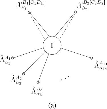
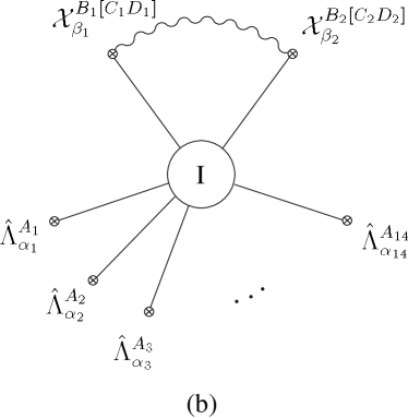
Figure 6: The two types of contributions to the correlation function (139). The notation is the same used in previous sections.

We first consider $G^{\rm(a)}_{\Lambda^{14}{\cal X}^{2}}$, see figure 6(a), which using the formulae of appendix D is given by

$$\hat{G}^{\rm(a)}_{\hat{\Lambda}^{14}{\cal X}^{2}} \!=\! \int d\mu_{\rm phys}\,{\rm e}^{-S_{4F}}\left[\hat{\Lambda}^{A_{1}}_{{\alpha}_{1}}(x_{1})\ldots\hat{\Lambda}^{A_{14}}_{{\alpha}_{14}}(x_{14}){\cal X}^{B_{1}[C_{1}D_{1}]}_{\beta_{1}}(y_{1}){\cal X}^{B_{2}[C_{2}D_{2}]}_{\beta_{2}}(y_{2})\right]$$

$$\!=\! \frac{1}{g_{{}_{\rm YM}}^{32}}\int d\mu_{\rm phys}\,{\rm e}^{-S_{4F}}\prod_{i=1}^{14}\frac{\rho^{4}}{[(x_{i}-x_{0})^{2}+\rho^{2}]^{4}}\zeta^{A_{i}}_{{\alpha}_{i}}$$

$$\hskip 95.3169pt\prod_{j=1}^{2}\left(\frac{\rho^{2}}{[(y_{j}-x_{0})^{2}+\rho^{2}]^{3}}\zeta^{D_{j}}\bar{\nu}^{(B_{j}}\nu^{C_{j})}-(C_{j}\leftrightarrow D_{j})\right)\,.$$

It can easily be argued that this term vanishes by the following symmetry argument. The whole expression must be a $SU(4)$ singlet. The integration over the $\bar{\nu}$ and $\nu$ modes factorises and therefore the indices carried by these variables must be combined to form a $SU(4)$ singlet separately. This is, however, not possible because (7.1) only contains $(\bar{\nu}\nu)_{\bf 10}$ bilinears and the product ${\bf 10}\otimes{\bf 10}={\bf 20^{\prime}}_{s}\oplus{\bf 35}_{s}\oplus{\bf 45}_{a}$ does not contain the singlet. Hence the whole expression vanishes.

Now consider the contribution $G^{\rm(b)}_{\Lambda^{14}{\cal X}^{2}}$ corresponding to the process in figure 6(b). We want to contract two $\varphi$’s in the ${\cal X}$ operators with a propagator instead of replacing them with their instanton profiles. In other words, we want to consider

$$\hat{G}^{\rm(b)}_{\hat{\Lambda}^{14}{\cal X}^{2}} \!=\! \frac{1}{g_{{}_{\rm YM}}^{32}}\langle{\rm Tr}\left(F_{m_{1}n_{1}}\sigma^{m_{1}n_{1}}_{\>{\alpha}_{1}}{}^{\gamma_{1}}\lambda^{A_{1}}_{\gamma_{1}}\right)(x_{1})\ldots{\rm Tr}\left(F_{m_{14}n_{14}}\sigma^{m_{14}n_{14}}_{\>{\alpha}_{14}}{}^{\gamma_{14}}\lambda^{A_{14}}_{\gamma_{14}}\right)(x_{14})$$ (142)

$$\left[4{\rm Tr}\left(\lambda^{B_{1}}_{\beta_{1}}\varphi^{C_{1}D_{1}}\right)(y_{1})\,{\rm Tr}\left(\lambda^{B_{2}}_{\beta_{2}}\varphi^{C_{2}D_{2}}\right)(y_{2})+\cdots\right]\rangle\;,\raisebox{-10.0pt}{ \rule{0.6pt}{4.0pt}\rule{94.74773pt}{0.6pt}\rule{0.6pt}{4.0pt}}$$

where the dots in the last line stand for eight other terms with the same structure obtained from the expansion of the product of the two ${\cal X}$’s and we will omit them in the next equations. Expanding the last equation and using (53) for the scalar propagator we find

$$\hat{G}^{\rm(b)}_{\hat{\Lambda}^{14}{\cal X}^{2}} = \frac{1}{g_{{}_{\rm YM}}^{32}}\langle{\rm Tr}\left(F_{m_{1}n_{1}}\sigma^{m_{1}n_{1}}_{{\alpha}_{1}}{}^{\gamma_{1}}\lambda^{A_{1}}_{\gamma_{1}}\right)(x_{1})\ldots{\rm Tr}\left(F_{m_{14}n_{14}}\sigma^{m_{14}n_{14}}_{{\alpha}_{14}}{}^{\gamma_{14}}\lambda^{A_{14}}_{\gamma_{14}}\right)(x_{14})$$ (143)

$$\frac{g_{{}_{\rm YM}}^{2}\varepsilon^{C_{1}D_{1}C_{2}D_{2}}}{4\pi^{2}}\left[\frac{2}{(y_{1}-y_{2})^{2}}{\rm Tr}\left({\cal P}(y_{2})\lambda^{B_{1}}_{\beta_{1}}(y_{1}){\cal P}(y_{1})\lambda^{B_{2}}_{\beta_{2}}(y_{2})\right)\right.$$

$$\left.+\frac{1}{\rho^{2}}{\rm Tr}\left({\cal P}(y_{1})b\bar{b}\lambda^{B_{1}}_{\beta_{1}}(y_{1})\right)\,{\rm Tr}\left({\cal P}(y_{2})b\bar{b}\lambda^{B_{1}}_{\beta_{1}}(y_{2})\right)\right]\rangle\,.$$

Notice that the terms proportional to $1/N$ and $1/N^{2}$ in the scalar propagator (53) do not contribute here because of the tracelessness of the elementary fields. Using the explicit expressions for the instanton profiles of the fields and for the ADHM matrices ${\cal P}$, $b$ and $\bar{b}$ given in the appendices we find

$${\rm Tr}\left[{\cal P}(y)b\bar{b}\lambda^{B_{1}}_{\beta_{1}}(y)\right]=0\,,$$ (144)

so that the contact term that would arise from the last line in (143) vanishes. The evaluation of the term in the second line is rather lengthy, but straightforward. It yields two types of contributions. After combining the results of the various contractions and reintroducing the numerical factors from the measure we find

$$\hat{G}^{\rm(b)}_{\hat{\Lambda}^{14}{\cal X}^{2}}=c(N)\frac{2^{46}3^{16}\varepsilon^{C_{1}D_{1}C_{2}D_{2}}{\rm e}^{2\pi i\tau}}{\pi^{31/2}g_{{}_{\rm YM}}^{22}}\int\frac{d\rho\,d^{4}x_{0}}{\rho^{5}}\prod_{A=1}^{4}d^{2}\eta^{A}\,d^{2}{\bar{\xi}}^{A}\prod_{i=1}^{14}\frac{\rho^{4}}{[(x_{i}-x_{0})^{2}+\rho^{2}]^{4}}\zeta^{A_{i}}_{{\alpha}_{i}}$$

$$\left[\prod_{j=1}^{2}\left(\frac{2}{(y_{1}-y_{2})^{2}}\frac{\rho^{2}}{[(y_{j}-x_{0})^{2}+\rho^{2}]^{2}}\zeta^{B_{j}}_{\beta_{j}}+\frac{\rho^{3}}{[(y_{j}-x_{0})^{2}+\rho^{2}]^{3}}\zeta^{B_{j}}_{\beta_{j}}\right)\right]+\cdots\,,$$ (145)

where

$$c(N)=N^{1/2}\left(1-\frac{5}{8N}+O(1/N^{2})\right)\,.$$ (146)

Therefore the correlation function $\hat{G}_{\hat{\Lambda}^{14}{\cal X}^{2}}$ has a leading contribution of order $N^{1/2}$ as expected, since it is related to AdS amplitudes involving interactions of order $({\alpha^{\prime}})^{-1}$. The spatial dependence in (145) is, however, different from that found in minimal correlators. In all the cases studied in [5, 6] the correlation functions took the form of contact contributions. Here there is a term of this type (the last one in $\hat{G}_{\hat{\Lambda}^{14}{\cal X}^{2}}^{\rm(b)}$) as well as a term with a different structure with a factorised $(y_{1}-y_{2})^{-2}$.

Now we will show how the above result agrees with the result of the calculation of the corresponding AdS amplitude. On the supergravity side there are two types of contributions as well. There is an obvious contribution from a diagram involving the D-instanton induced part of the coupling arising from the ten-dimensional vertex

$$\frac{1}{{\alpha^{\prime}}}\int d^{10}x\sqrt{-g}\,{\rm e}^{-\phi/2}f_{1}^{(11,-11)}(\tau,\bar{\tau})\Lambda^{14}{\bar{\psi}}^{*}\gamma\psi\,.$$ (147)

Taking the vector indices of the gravitini in $S^{5}$ directions produces a five-dimensional coupling that generates a contact diagram contributing to the amplitude dual to the correlation function we are considering, see figure 7(a).

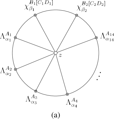
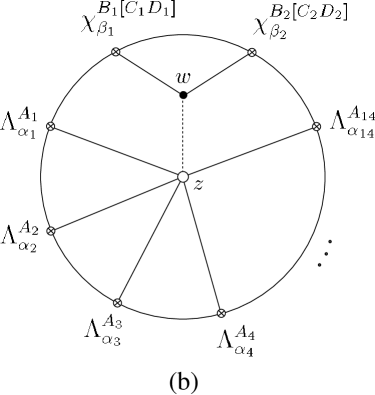
Figure 7: The two AdS amplitudes contributing to $G_{\Lambda^{14}\chi^{2}}$.

The resulting amplitude is straightforward to evaluate and yields

$$G^{\rm(a)}_{\Lambda^{14}\chi^{2}}=c_{\rm a}(\tau,\bar{\tau},N)\int\frac{d^{5}z}{z_{0}^{5}}\prod_{i=1}^{14}K_{7/2}^{F}(z;x_{i})\prod_{j=1}^{2}K_{5/2}^{F}(z;y_{j})\,,$$ (148)

where, at leading order, the coefficient $c(\tau,\bar{\tau},N)$ is

$$c_{\rm a}(\tau,\bar{\tau},N)=c_{\rm a}N^{1/2}g_{\rm s}^{-11}{\rm e}^{2\pi i\tau}+O(N^{-1/2})\,.$$ (149)

In (148) the usual notation for bulk-to-boundary propagators has been used: $K_{7/2}^{F}$ was defined in (104), whereas the two gravitini have been replaced by

$$K^{F}_{5/2}(z_{m},z_{0};x_{m}) = K_{3}(z_{m},z_{0};x_{m})\frac{1}{\sqrt{z_{0}}}\left(z_{0}\gamma_{\hat{5}}+(z-x)^{m}\gamma_{\hat{m}}\right)$$ (150)

$$= \frac{z_{0}^{3}}{[(z-x)^{2}+z_{0}^{2}]^{3}}\frac{1}{\sqrt{z_{0}}}\left(z_{0}\gamma_{\hat{5}}+(z-x)^{m}\gamma_{\hat{m}}\right)\,.$$

There is a second AdS amplitude that contributes to the same process. This is an exchange amplitude of the type of those considered in section 5.2. The process we have to consider here involves a D-instanton induced vertex $f_{1}^{(11,-11)}(\tau,\bar{\tau})\Lambda^{14}G$ with the $G$ splitting into two $\psi$’s via a classical cubic interaction $\bar{G}\psi\psi$ where the spatial indices are in internal directions. This amplitude is represented in figure 7(b). The dotted line is a bulk-to-bulk propagator for a scalar associated with internal components of $G$. Analysing the spectrum of scalars in [31] we see that the allowed states are the Kaluza–Klein ground state which is in the ${\bf 10}$ of $SU(4)$ and the second excited state, in the ${\bf 50}$. The corresponding couplings are superconformal descendants of a next-to-extremal and an extremal coupling respectively. Although the relevant integrals, involving fermions, are not among the cases studied in the literature we expect the extremal diagram to reduce to a contribution of the form of (148)

$$G^{\rm(b1)}_{\Lambda^{14}\chi^{2}}=c_{\rm b1}(\tau,\bar{\tau},N)\int\frac{d^{5}z}{z_{0}^{5}}\prod_{i=1}^{14}K_{7/2}^{F}(z;x_{i})\prod_{j=1}^{2}K_{5/2}^{F}(z;y_{j})\,,$$ (151)

where

$$c_{\rm b1}(\tau,\bar{\tau},N)=c_{\rm b1}N^{1/2}g_{\rm s}^{-11}{\rm e}^{2\pi i\tau}+O(N^{-1/2})\,.$$ (152)

Analogously the next-to-extremal diagram is expected to give

$$G^{\rm(b2)}_{\Lambda^{14}\chi^{2}}=\frac{c_{\rm b2}(\tau,\bar{\tau},N)}{(y_{1}-y_{2})^{2}}\int\frac{d^{5}z}{z_{0}^{5}}\prod_{i=1}^{14}K_{7/2}^{F}(z;x_{i})\prod_{j=1}^{2}K_{3/2}^{F}(z;y_{j})\,,$$ (153)

where

$$K^{F}_{3/2}(z_{m},z_{0};x_{m}) = K_{2}(z_{m},z_{0};x_{m})\frac{1}{\sqrt{z_{0}}}\left(z_{0}\gamma_{\hat{5}}+(z-x)^{m}\gamma_{\hat{m}}\right)$$ (154)

$$= \frac{z_{0}^{2}}{[(z-x)^{2}+z_{0}^{2}]^{2}}\frac{1}{\sqrt{z_{0}}}\left(z_{0}\gamma_{\hat{5}}+(z-x)^{m}\gamma_{\hat{m}}\right)$$

and

$$c_{\rm b2}(\tau,\bar{\tau},N)=c_{\rm b2}N^{1/2}g_{\rm s}^{-11}{\rm e}^{2\pi i\tau}+O(N^{-1/2})\,.$$ (155)

Let us now compare the AdS result with what we obtained from the Yang–Mills calculation. The two terms (148) and (151) have the structure of contact contributions. They reproduce the last term in the Yang–Mills result of (145). From a five-dimensional point of view these two contributions would not be distinguished. Proceeding as in perturbative calculations (for example, as in the analysis in [12]) the process in figure 7(b) would not be included, but its effect would result from the correction it induces in the five-dimensional $\Lambda^{14}\hat{G}$ coupling. The AdS amplitude involving the next-to-extremal interaction (153) agrees exactly with the remaining term in (145). The $SU(4)$ tensor in the Yang–Mills result is obtained from the integration over the five-sphere analogously to the cases analysed in previous sections. In conclusion we find agreement at order $N^{1/2}$ between the two calculations. This example illustrates how the different effects described in this paper are relevant even for processes arising at the level of the leading instanton corrections.

7.2 Other higher derivative interactions in type IIB string theory

In section 5 we discussed the details of how the instanton contribution to a correlation function with sixteen $\hat{\Lambda}$’s and two ${\cal Q}_{2}$’s can be computed in the semiclassical approximation. This was related via the AdS/CFT correspondence to higher derivative interactions in string theory at order ${\alpha^{\prime}}^{-1}$ and ${\alpha^{\prime}}$. We will now consider other examples of this kind that involve the correlation functions

$$\hat{G}_{\hat{\Lambda}^{16}{\cal E}^{4}}(x_{1},\ldots,x_{16},y_{1},\ldots,y_{4})\!=\!\langle\hat{\Lambda}^{A_{1}}_{{\alpha}_{1}}(x_{1})\ldots\hat{\Lambda}^{A_{16}}_{{\alpha}_{16}}(x_{16}){\cal E}^{B_{1}C_{1}}(y_{1})\ldots{\cal E}^{B_{4}C_{4}}(y_{4})\rangle$$ (156)

and

$$\hat{G}_{\hat{\Lambda}^{16}{\cal B}^{4}}(x_{1},\ldots,x_{16},y_{1},\ldots,y_{4})\!=\!\langle\hat{\Lambda}^{A_{1}}_{{\alpha}_{1}}(x_{1})\ldots\hat{\Lambda}^{A_{16}}_{{\alpha}_{16}}(x_{16}){\cal B}^{B_{1}C_{1}}_{m_{1}n_{1}}(y_{1})\ldots{\cal B}^{B_{4}C_{4}}_{m_{4}n_{4}}(y_{4})\rangle.$$ (157)

As observed after (138), in the AdS/CFT correspondence ${\cal E}^{(AB)}$ and ${\cal B}^{[AB]}_{mn}$ are the composite operators in the supercurrent multiplet associated with the internal and space-time components of the complex combination of the $NS\otimes NS$ and $R\otimes R$ two-forms in supergravity. A naive generalisation of the analysis of [5, 6] would associate the above correlation functions with terms in the type IIB effective action of the form ${\alpha^{\prime}}\,G^{4}\,\Lambda^{16}$, which were discussed in (2) in section 2. This specific interaction has been recently studied in detail in [43]. As before, the reason for considering the particular correlation functions in (156) and (157) is that the analysis is simpler for the terms with the maximal number of fermions.

In the semiclassical approximation the classical solutions of section 4.1 are used to saturate the integrations over the fermion zero-modes. Each operator $\hat{\Lambda}^{A}_{\alpha}$ soaks up one superconformal mode and does not depend on the additional modes $\bar{\nu}$ and $\nu$. The operators ${\cal E}^{AB}$ and ${\cal B}^{AB}_{mn}$ each soak up two zero modes, but in the case of ${\cal B}^{AB}_{mn}$ these are necessarily superconformal modes as follows from the classical expression (278). Thus there is a non-vanishing contribution to the correlation function (156) in which the sixteen exact fermion modes come from the $\hat{\Lambda}$’s and each ${\cal E}$ gives a bilinear $(\bar{\nu}\nu)_{\bf 10}$ in the $\nu$’s, but no similar contribution can exist for (157). There is, however, a different type of contribution to (157) which is non-zero and comes from considering the ${\rm Tr}(\varphi^{AB}F_{mn})$ term in the operator ${\cal B}^{AB}_{mn}$ (60). The new contribution is obtained by contracting a scalar field, $\varphi$, in one of the ${\cal B}^{AB}_{mn}$ operators with a propagator joining it to another ${\cal B}^{AB}_{mn}$ operator. The remaining $F_{mn}$’s in each ${\cal B}$ are substituted by their non-vanishing value in the instanton background. As in previous examples only scalar contractions are possible because of the chirality of the fermions and the self-duality of the field strength. This means that there is no analogous contribution involving propagators to the correlation function (156) with ${\cal E}$ insertions at leading order in the coupling $g_{{}_{\rm YM}}$.

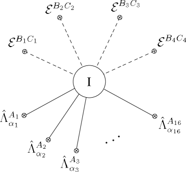
Figure 8: Instanton contribution to the correlation function (156).

First consider the ‘purely instantonic’ process which gives rise to (156). This is represented diagrammatically in figure 8. In the semiclassical approximation the result is

$$\hat{G}_{\hat{\Lambda}^{16}{\cal E}^{4}}=\int d\mu_{\rm phys}\,{\rm e}^{-S_{4F}}\left[\hat{\Lambda}^{A_{1}}_{{\alpha}_{1}}(x_{1})\ldots\hat{\Lambda}^{A_{16}}_{{\alpha}_{16}}(x_{16})\,{\cal E}^{B_{1}C_{1}}(y_{1})\ldots{\cal E}^{B_{2}C_{2}}(y_{4})\right]$$

$$=\frac{1}{g_{{}_{\rm YM}}^{40}}\int d\mu_{\rm phys}\,{\rm e}^{-S_{4F}}\left[\prod_{i=1}^{16}\frac{\rho^{4}\zeta^{A_{i}}_{{\alpha}_{i}}}{[(x_{i}-x_{0})^{2}+\rho^{2}]^{4}}\prod_{j=1}^{4}\frac{\rho^{2}({\bar{\nu}}^{B_{j}u}\nu^{C_{j}}_{u}+{\bar{\nu}}^{C_{j}u}\nu^{B_{j}}_{u})}{[(y_{j}-x_{0})^{2}+\rho^{2}]^{3}}\right]\,,$$ (158)

where we have substituted the classical expressions for the operators $\hat{\Lambda}$ and ${\cal E}$ which are given by (276) and (277), respectively. The combinatorics necessary to evaluate the $2(N-2)$ fermionic integrations over $\bar{\nu}^{Au}$ and $\nu^{A}_{u}$ is simplified with the aid of the generating function defined earlier in section 3.2. After some algebra the result is

$$\hat{G}_{\hat{\Lambda}^{16}{\cal E}^{4}} \!=\! c(N)t^{B_{1}C_{1}\ldots B_{4}C_{4}}\frac{2^{40}3^{16}{\rm e}^{2\pi i\tau}}{\pi^{35/2}g_{{}_{\rm YM}}^{28}}\int\frac{d\rho\,d^{4}x_{0}}{\rho^{5}}\prod_{A=1}^{4}d^{2}\eta^{A}\,d^{2}{\bar{\xi}}^{A}\>$$ (159)

$$\left[\prod_{i=1}^{16}\frac{\rho^{4}}{[(x_{i}-x_{0})^{2}+\rho^{2}]^{4}}\zeta^{A_{i}}_{{\alpha}_{i}}\prod_{j=1}^{4}\frac{\rho^{3}}{[(y_{j}-x_{0})^{2}+\rho^{2}]^{3}}\right]\,,$$

where

$$c(N)=N^{1/2}\left(1-\frac{25}{8N}+O(1/N^{2})\right)$$ (160)

and the tensor $t^{B_{1}C_{1}\ldots B_{4}C_{4}}$, determined by the five-sphere integration, takes the form

$$t^{B_{1}C_{1}\ldots B_{4}C_{4}} = \left(\varepsilon^{B_{1}B_{2}B_{3}B_{4}}\varepsilon^{C_{1}C_{2}C_{3}C_{4}}+\varepsilon^{B_{1}C_{2}C_{3}C_{4}}\varepsilon^{C_{1}B_{2}B_{3}B_{4}}\right.$$ (161)

$$\left.+~{}{\rm 6~{}terms~{}obtained~{}by~{}symmetrisation~{}in~{}}(B_{i},C_{i})~{}\right)\,.$$

We would like to compare this expression with the corresponding supergravity process. With the usual identification, $\left((x_{0})_{m},\rho\right)\longleftrightarrow(z_{m},z_{0})$, and recalling (66), we notice that the integrand in (159) contains sixteen factors that correspond to the dilatini bulk-to-boundary propagators and four factors of the bulk-to-boundary propagator $K_{3}$, which is the propagator for a scalar field of dimension $\Delta=3$. The supergravity scalar field, $E^{AB}$, that couples to ${\cal E}^{AB}$ in (159) comes from the second-rank potential, $B_{\alpha\beta}$, which has indices in the five-sphere directions. The leading term (of order $N^{1/2}$) in the expression for $\hat{G}_{\hat{\Lambda}^{16}{\cal E}^{4}}$ (159) therefore appears to correspond to a contact interaction of the form $({\alpha^{\prime}})^{-1}\,\Lambda^{16}\,E^{4}$. Such a term does not arise among the interactions of order $({\alpha^{\prime}})^{-1}$ in ten dimensions (indeed, it is not even gauge invariant). Nevertheless an amplitude with exactly the same structure emerges from an AdS tree level process involving a $\Lambda^{16}$ D-instanton induced interaction. A contribution of the form of (159) results from a tree diagram in $AdS_{5}\times S^{5}$ with a D-instanton at one vertex. The coupling we need to consider here is of the form

$$\int d^{10}\sqrt{-g}{\rm e}^{-\phi/2}f_{1}^{(12,-12)}(\tau,\bar{\tau})\tau^{2}\Lambda^{16}$$ (162)

and it arises at order ${\alpha^{\prime}}^{-1}$ via the mechanism described in section 5 from the expansion of the ${\rm e}^{2\pi i\tau}$ factor. To obtain the amplitude relevant to our example each dilaton must couple to a pair of $G$’s via a $\bar{\tau}G^{2}$ vertex in the classical IIB supergravity. The amplitude is represented in figure 9(a). From the $AdS_{5}\times S^{5}$ point of view the allowed processes are all those compatible with the $SU(4)\sim SO(6)$ symmetry. Group theoretical restrictions imply that in this particular process the two intermediate dilatons can only be in the ${\bf 20^{\prime}}$ of $SU(4)$, i.e. they are in the second Kaluza-Klein excited state which will is denoted by $\tau_{20^{\prime}}$. This means that the cubic $\bar{\tau}GG$ vertices involved are extremal and as in previously described cases the process reduces to a contact amplitude that contributes at order $N^{1/2}$. This can be seen directly from the expression of the tree diagram with all the indices on the antisymmetric tensor potential $B_{\mu\nu}$ aligned along the five-sphere. Indeed, making use of the equations of motion in [31] it is easy to see that, after two integrations by parts, each of the cubic vertices can be written as the integral of $(\partial^{2}+m_{\tau_{20^{\prime}}})\bar{\tau}_{20^{\prime}}B_{ij}B^{ij}$, where the mass term comes from derivatives in $S^{5}$ directions. In this form, it is manifest that such a vertex cancels the adjacent $\langle\tau\bar{\tau}\rangle_{20^{\prime}}$ propagator.

This means that from a five-dimensional point of view this process appears to produce a new coupling at order ${\alpha^{\prime}}^{-1}$ of the form

$$g_{\rm s}^{-2}\int\frac{d^{5}z}{z_{0}^{5}}\,{\rm e}^{-\phi/2}f_{1}^{(12,-12)}(\tau,\bar{\tau})\Lambda^{16}E^{4}\,,$$ (163)

where the factor of $g_{\rm s}^{-2}$ is obtained after canonically normalising the kinetic term for the dilaton. The interaction (163) is not manifestly gauge invariant since it involves the field $E$ and not the field strength $G$. This is, however, not a problem because gauge invariance is recovered when (163) is combined with the other couplings, involving the antisymmetric tensor $B_{mn}$ and the vectors resulting from mixed components of the ten-dimensional two-form, which also descend from the tree level process just described.

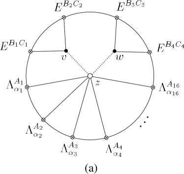
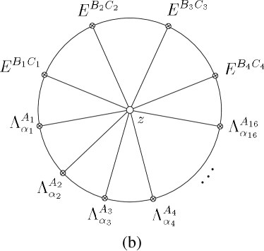
Figure 9: AdS amplitudes contributing to the process dual to the correlation function (156).

The same amplitude gets a contribution from the contact diagram generated by the $G^{4}\Lambda^{16}$ interaction that is expected to contribute at order ${\alpha^{\prime}}$. This is a higher order term, ${\alpha^{\prime}}$ with respect to the classical Einstein–Hilbert term, in the derivative expansion of the string effective action that was discussed in section 2. Notice that in this comparison a crucial rôle is played by the self-duality property of the complex type IIB two-form with indices in internal directions [31], which implies that the $AdS$ diagram involves $K_{3}$ bulk-to-boundary propagators for the $G$’s. This second contribution is of order $N^{-1/2}$ corresponding to a vertex of order ${\alpha^{\prime}}$. The situation at order $N^{-1/2}$ is actually more complicated. There is in fact another source of corrections at this order. At the end of section 3 we commented on how the $1/N$ corrections to the minimal correlation functions are reproduced in supergravity. In the case of the correlator of sixteen dilatini for example the order $N^{-1/2}$ effects are expected to arise from amplitudes involving the vertices

$${\alpha^{\prime}}\int d^{10}x\sqrt{-g}\,{\rm e}^{\phi/2}f_{2}^{(12,-12)}(\tau,\bar{\tau})\Lambda^{16}\left({\cal R}^{2}+F_{(5)}^{4}\right)\,,$$ (164)

where the ${\cal R}^{2}$ and $F_{(5)}^{4}$ factors are set to their non-vanishing background values. Analogously here we have to consider similar effects associated with (162), i.e. tree level processes in which the D-instanton vertex is

$${\alpha^{\prime}}\int d^{10}x\sqrt{-g}\,{\rm e}^{\phi/2}f_{2}^{(12,-12)}(\tau,\bar{\tau})\Lambda^{16}\tau^{2}\left({\cal R}^{2}+F_{(5)}^{4}\right)\,,$$ (165)

with ${\cal R}^{2}$ and $F_{(5)}^{4}$ taken to be constant. As for the leading $N^{1/2}$ term the resulting exchange diagrams contain extremal couplings of the dilatons with pairs of $G$’s and should produce again a contact contribution. Determining the correct coefficients of all the relevant terms is extremely subtle, so we will not go beyond a qualitative analysis. In conclusion we find that all the different effects just described give rise to the same structure and the complete AdS result reads

$$G_{\Lambda^{16}E^{4}}=c(\tau,\bar{\tau},N)\int\frac{d^{5}z}{z_{0}^{5}}\,\prod_{i=1}^{16}K^{F}_{7/2}(z;x_{i})\prod_{j=1}^{4}K_{3}(z;y_{j})\,,$$ (166)

where

$$c(\tau,\bar{\tau},N)=g_{\rm s}^{-14}{\rm e}^{2\pi i\tau}\left(c_{1}N^{1/2}+c_{2}N^{-1/2}\right)\,.$$ (167)

Notice that the common power of the string coupling has a different origin in the two terms in (167). In the leading order term and in the subleading correction produced by the amplitude induced by (165) the factor of $g_{\rm s}^{-14}$ is the combination of a $\tau_{2}^{12}$ from the modular form $f_{1}^{(12,-12)}(\tau,\bar{\tau})$ and two additional factors of $g_{\rm s}$ following from the proper normalisation of the kinetic term for the dilaton. In the subleading term generated by the $G^{4}\Lambda^{16}$ interaction the correct powers of the coupling constant come from the expansion of the modular form $f_{2}^{(14,-14)}(\tau,\bar{\tau})$ defined in (2) and (16). Comparing this result with the Yang–Mills expression (159) we find agreement up to numerical constants that we have not checked.

We now turn to the case of correlation functions with insertions of ${\cal B}^{[AB]}_{mn}$. A natural example to consider is (157) which naively would be expected to correspond to an AdS amplitude generated by the interaction $G^{4}\Lambda^{16}$ at order ${\alpha^{\prime}}$ with the indices on the $G$’s in AdS directions. In view of the previous discussion concerning the case of the correlation function $\hat{G}_{\hat{\Lambda}^{16}{\cal E}^{4}}$, however, we can consider the simpler case

$$\hat{G}_{\hat{\Lambda}^{16}{\cal B}^{2}}=\langle\hat{\Lambda}^{A_{1}}_{{\alpha}_{1}}(x_{1})\ldots\hat{\Lambda}^{A_{16}}_{{\alpha}_{16}}(x_{16}){\cal B}^{B_{1}C_{1}}_{m_{1}n_{1}}(y_{1}){\cal B}^{B_{2}C_{2}}_{m_{2}n_{2}}(y_{2})\rangle\,.$$ (168)

On the Yang–Mills side it is natural to expect a non-vanishing result for this correlation function since it is allowed by group theory: the indices on the sixteen $\hat{\Lambda}$’s are combined to form a $SU(4)$ singlet and a singlet is also contained in the product of two ${\bf 6}$’s corresponding to the ${\cal B}$ insertions. On the supergravity side there is no candidate vertex in the type IIB ten dimensional effective action in Minkowski space to generate an amplitude dual to (168). Nevertheless we expect to generate a $\Lambda^{16}B^{2}$ effective interaction in $AdS_{5}\times S^{5}$ at order ${\alpha^{\prime}}^{-1}$ via the same mechanism discussed in the case of (163).

The correlation function (168) is more complicated than previous examples because it involves antisymmetric tensors which lead to a non-trivial tensorial structure. The calculation is straightforward but tedious and we will discuss the general features of this correlator without deriving a complete explicit expression. The Yang–Mills and AdS diagrams corresponding to (168) are depicted in figure 10.

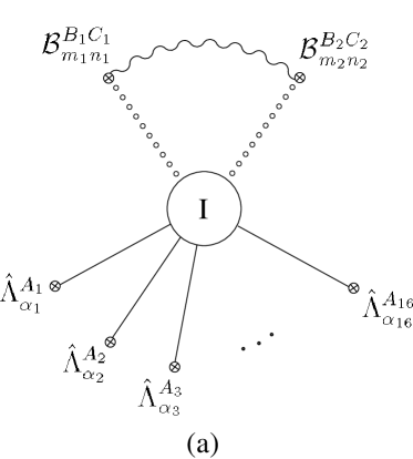
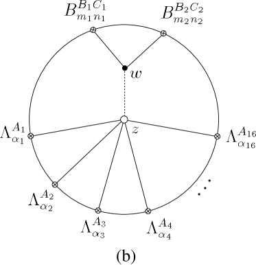
Figure 10: Diagram (a) represents the Yang–Mills contribution to the correlation function (168). The lines denoted by small circles in (a) indicate insertions of $F_{m_{i}n_{i}}$, which do not contain fermionic modes, but have a non vanishing value in the instanton background. Diagram (b) represents the AdS amplitude contributing to the dual process.

Since the ${\cal B}^{BC}_{mn}$ fields do not depend on the $\nu$ and $\bar{\nu}$ modes, contractions between pairs of scalar fields in the ${\cal B}$ insertions must be considered to get a non-vanishing result. This gives

$$\hat{G}_{\hat{\Lambda}^{16}{\cal B}^{2}}(x_{1},\ldots,x_{16},y_{1},y_{2})=\langle\hat{\Lambda}^{A_{1}}_{{\alpha}_{1}}(x_{1})\ldots\hat{\Lambda}^{A_{16}}_{{\alpha}_{16}}(x_{16}){\cal B}^{B_{1}C_{1}}_{m_{1}n_{1}}(y_{1})\ldots{\cal B}^{B_{4}C_{4}}_{m_{4}n_{4}}(y_{4})\rangle$$ (169)

$$=\frac{1}{g_{{}_{\rm YM}}^{36}}\langle{\rm Tr}\left(F_{m_{1}n_{1}}\sigma^{m_{1}n_{1}}_{{\alpha}_{1}}{}^{\beta_{1}}\lambda^{A_{1}}_{\beta_{1}}\right)(x_{1})\ldots{\rm Tr}\left(2i\varphi^{B_{1}C_{1}}F_{p_{1}q_{1}}\right)(y_{1}){\rm Tr}\left(2i\varphi^{B_{2}C_{2}}F_{p_{2}q_{2}}\right)(y_{2})\raisebox{-10.0pt}{ \rule{0.6pt}{4.0pt}\rule{104.70593pt}{0.6pt}\rule{0.6pt}{4.0pt}}\hskip 75.11525pt\rangle\,.$$

Let us compute the contraction in (169) separately. Using the scalar propagator (53) we get

$${\rm Tr}\left(2i\varphi^{B_{1}C_{1}}F_{p_{1}q_{1}}\right)(y_{1}){\rm Tr}\left(2i\varphi^{B_{2}C_{2}}F_{p_{2}q_{2}}\right)(y_{2})\raisebox{-10.0pt}{ \rule{0.6pt}{4.0pt}\rule{104.70593pt}{0.6pt}\rule{0.6pt}{4.0pt}}$$

$$=\frac{g_{{}_{\rm YM}}^{2}\varepsilon^{B_{1}C_{1}B_{2}C_{2}}}{2\pi^{2}}\left[\frac{1}{(y_{1}-y_{2})^{2}}{\rm Tr}\left({\cal P}(x_{2})F_{m_{1}n_{1}}(x_{1}){\cal P}(x_{1})F_{m_{2}n_{2}}(x_{2})\right)\right.$$

$$\left.+\frac{1}{2\rho^{2}}{\rm Tr}\left(\bar{b}F_{m_{1}n_{1}}(x_{1}){\cal P}(x_{1})b\right){\rm Tr}\left(\bar{b}F_{m_{2}n_{2}}(x_{2}){\cal P}(x_{2})b\right)\right]\,,$$ (170)

where we have used the tracelessness of $F_{mn}$ to discard the contribution of the $1/N$ and $1/N^{2}$ terms in the propagator. It is easy to verify that the terms in the last line of (170) vanish, so that for (169) we obtain

$$\hat{G}_{\hat{\Lambda}^{16}{\cal B}^{2}}=\frac{g_{{}_{\rm YM}}^{2}\varepsilon^{B_{1}C_{1}B_{2}C_{2}}}{2\pi^{2}(y_{1}-y_{2})^{2}}\,\langle\hat{\Lambda}^{A_{1}}_{{\alpha}_{1}}(x_{1})\ldots\hat{\Lambda}^{A_{16}}_{{\alpha}_{16}}(x_{16}){\rm Tr}\left[{\cal P}(y_{2})F_{m_{1}n_{1}}(y_{1}){\cal P}(y_{1})F_{m_{2}n_{2}}(y_{2})\right]\rangle\,.$$ (171)

Evaluating this expression in the instanton background leads to the result

$$\hat{G}_{\hat{\Lambda}^{16}{\cal B}^{2}} = c(N)\frac{\varepsilon^{B_{1}C_{1}B_{2}C_{2}}2^{40}3^{16}{\rm e}^{2\pi i\tau}}{\pi^{31/2}g_{{}_{\rm YM}}^{26}}\int\frac{d\rho\,d^{4}x_{0}}{\rho^{5}}\prod_{A=1}^{4}d^{2}\eta^{A}\,d^{2}{\bar{\xi}}^{A}\prod_{i=1}^{16}\frac{\rho^{4}}{[(x_{i}-x_{0})^{2}+\rho^{2}]^{4}}\zeta^{A_{i}}_{{\alpha}_{i}}$$ (172)

$$\left\{\left[\frac{1}{(y_{1}-y_{2})^{2}}\prod_{j=1}^{2}\frac{\rho^{2}}{[(y_{j}-x_{0})^{2}+\rho^{2}]^{2}}\right.\right.$$

$$\left.\left.-\prod_{j=1}^{2}\frac{\rho^{3}}{[(y_{j}-x_{0})^{2}+\rho^{2}]^{3}}\right]{\rm tr}(\sigma_{m_{1}n_{1}}\sigma_{m_{2}n_{2}})+\cdots\right\}\,,$$

i.e. as in previous cases we obtain a term with the structure of a contact contribution as well as a term with a factorised $(y_{1}-y_{2})^{-2}$. The $\cdots$ in (172) denotes terms with different tensor structure. The $N$-dependence is contained in the prefactor

$$c(N)=N^{1/2}\left(1-\frac{5}{8N}+O(1/N^{2})\right)\,.$$ (173)

The result can now be compared with the expectations from the supergravity calculation. In order to understand the AdS side of the correspondence for this process it is necessary to consider the amplitude in figure 10(b). This is a tree diagram in which the vertex in $z$ is a D-instanton induced interaction coupling sixteen dilatini to a dilaton. In this case the dilaton couples to a pair of $B_{mn}$’s, with indices in AdS directions, which are in the 6 of $SU(4)$. There are two kinds of allowed contributions. These arise from the possibility of the dilaton being in its massless Kaluza–Klein ground state, which is a singlet of $SU(4)$ or in its second Kaluza–Klein state, which is a ${\bf 20^{\prime}}$ of $SU(4)$. The evaluation of the integrals entering these amplitudes is complicated because of the presence of the antisymmetric tensors. The vertices in the two cases (dilaton in the ${\bf 1}$ or ${\bf 20^{\prime}}$) are superconformal descendants of a next-to-extremal and an extremal coupling respectively. Hence we expect the amplitude in the case of singlet exchange to reduce to

$$G_{\Lambda^{16}B^{2}}^{\rm(1)}=\frac{c_{1}(\tau,\bar{\tau},N)}{(y_{1}-y_{2})^{2}}\int\frac{d^{5}z}{z_{0}^{5}}\prod_{i=1}^{16}K_{7/2}^{F}(z;x_{i})\prod_{j=1}^{2}K_{2;m_{j}n_{j}}(z;y_{j})\,,$$ (174)

whereas for the ${\bf 20^{\prime}}$ exchange we expect

$$G_{\Lambda^{16}B^{2}}^{\rm(2)}=c_{2}(\tau,\bar{\tau},N)\int\frac{d^{5}z}{z_{0}^{5}}\prod_{i=1}^{16}K_{7/2}^{F}(z;x_{i})\prod_{j=1}^{2}K_{3;m_{j}n_{j}}(z;y_{j})\,.$$ (175)

In both cases the prefactors have a leading contribution of order $N^{1/2}$ plus $1/N$ corrections

$$c_{i}(\tau,\bar{\tau},N)=c_{i}g_{\rm s}^{-13}{\rm e}^{2\pi i\tau}\left(N^{1/2}+O(N^{-1/2})\right)\,,\quad i=1,2\,,$$ (176)

where the powers of the string coupling come from the $f_{1}^{(12,-12)}(\tau,\bar{\tau})$ in the $\Lambda^{16}$ vertex and the normalisation of the dilaton fluctuations. In these expressions $K_{\Delta;mn}(z;x)$ denotes the bulk-to-boundary propagator for an antisymmetric tensor dual to an operator of dimension $\Delta$ [44], which has AdS mass squared $m^{2}L^{2}=\Delta^{2}-4\Delta+3$. The product of the two $K_{\Delta;mn}$’s in (174) and (175) contains several terms, in particular

$$\prod_{j=1}^{2}K_{\Delta;m_{j}n_{j}}(z;y_{j})=\prod_{j=1}^{2}K_{\Delta}(z;y_{j})\,{\rm tr}(\sigma_{m_{1}n_{1}}\sigma_{m_{2}n_{2}})+\cdots\,,$$ (177)

so that the AdS result reproduces qualitatively the correct terms in the Yang–Mills calculation.

A comment can be added about the comparison with the five-dimensional perspective. In a five-dimensional approach only the singlet exchange diagram would be included, but the effective action would then contain a genuine new interaction of the form

$$g_{\rm s}^{-1}\int\frac{d^{5}z}{z_{0}^{5}}\,{\rm e}^{-\phi/2}f_{1}^{(12,-12)}(\tau,\bar{\tau})\Lambda^{16}B^{2}\,,$$ (178)

producing the amplitude (175). Again, gauge invariance of the complete effective action results from combining (178) with vertices containing vector fields.

The effects just described in the case of the correlator (168) are the building blocks for the evaluation of (157). In this case the contact term at order $N^{-1/2}$ gets also an additional contribution from a diagram with a $\Lambda^{16}G^{4}$ vertex at order ${\alpha^{\prime}}$ with indices on the $G$’s in $AdS_{5}$ directions.

More generally we can consider correlation functions of the form

$$\hat{G}_{\hat{\Lambda}^{16}{\cal E}^{2k}}=\langle\hat{\Lambda}^{A_{1}}_{{\alpha}_{1}}(x_{1})\ldots\hat{\Lambda}^{A_{16}}_{{\alpha}_{16}}(x_{16})\,{\cal E}^{(B_{1}C_{1})}(y_{1})\ldots{\cal E}^{(B_{2k}C_{2k})}(y_{2k})\rangle$$ (179)

$$\hat{G}_{\hat{\Lambda}^{16}{\cal B}^{2k}}=\langle\hat{\Lambda}^{A_{1}}_{{\alpha}_{1}}(x_{1})\ldots\hat{\Lambda}^{A_{16}}_{{\alpha}_{16}}(x_{16})\,{\cal B}_{m_{1}n_{1}}^{[B_{1}C_{1}]}(y_{1})\ldots{\cal B}_{m_{2k}n_{2k}}^{[B_{2k}C_{2k}]}(y_{2k})\rangle\,.$$ (180)

These correlation functions are naturally associated (for even $k$) with a class of terms in the type IIB effective action which were conjectured in [14]. In that paper terms of the form ${\cal R}^{4}G^{4g-4}$ were conjectured to arise at order $({\alpha^{\prime}})^{2g-3}$ in flat space. On the other hand a generalisation of the Yang–Mills calculations of this section leads us to expect all the non-vanishing correlation functions of the form (179) and (180) to have a leading contribution of order $N^{1/2}$, i.e. $({\alpha^{\prime}})^{-1}$ in terms of string parameters. It is particularly easy to convince oneself that this is the case for (179) using the general formulae of section 3.2. We have seen that each ${\cal E}$ contains only a bilinear $(\bar{\nu}\nu)_{\bf 10}$, so that (179) involves $2k$ $(\bar{\nu}\nu)_{\bf 10}$ and no $(\bar{\nu}\nu)_{\bf 6}$ insertions. Using the general formula (44) we then conclude that

$$\hat{G}_{\hat{\Lambda}^{16}{\cal E}^{2k}}\sim g_{{}_{\rm YM}}^{-24-k}{\rm e}^{2\pi i\tau}N^{1/2}\,.$$ (181)

To explain this mismatch in powers of $N$ we need to consider AdS amplitudes like the ones producing the leading contribution in the case of $\hat{G}_{\hat{\Lambda}^{16}{\cal E}^{4}}$. For the general correlation function (179) the AdS diagrams to be computed are generalised processes of the type in figure 9(a), involving the vertex

$$\frac{1}{{\alpha^{\prime}}}\int d^{10}x\sqrt{-g}\,{\rm e}^{-\phi/2}f_{1}^{(12,-12)}(\tau,\bar{\tau})\Lambda^{16}\tau^{k}\,.$$ (182)

and $k$ $\bar{\tau}G^{2}$ classical cubic interactions. A process of this type will indeed produce a dependence in agreement with (181). The conclusion is that a test of the conjectures of [14] using the methods of the present paper is impossible, because the effects of the interactions proposed in [14] are subleading and highly suppressed in the large-$N$ expansion in $AdS_{5}\times S^{5}$.

7.3 Near extremal correlation functions

Among the most striking new results in ${\cal N}=4$ SYM which were stimulated by results in supergravity via the AdS/CFT correspondence is the non-renormalisation of a class of $n$-point functions, the extremal and next-to-extremal correlation functions of chiral primary operators [34, 35, 36, 37, 38]. These are functions of the type

$$G_{n}(x_{1},x_{2},\ldots,x_{n})=\langle{\cal Q}_{\ell_{1}}(x_{1}){\cal Q}_{\ell_{2}}(x_{1})\ldots{\cal Q}_{\ell_{n}}(x_{n})\rangle\,,$$ (183)

where $\ell_{1}=\sum_{i=2}^{n}\ell_{i}$ in the extremal case and $\ell_{1}+2=\sum_{i=2}^{n}\ell_{i}$ in the next-to-extremal case. For all the $G_{n}$’s of this type supergravity predicts the absence of quantum corrections to the free theory result and this prediction has been checked by explicit calculations in ${\cal N}=4$ SYM. In particular, correlation functions in this class do not receive instanton corrections [35, 38].

An even more interesting set of correlation functions are the near-extremal ones [12], for which $\ell_{1}+2m=\sum_{i=2}^{n}\ell_{i}$, with $m\geq 2$, in (183). The near-extremal functions do receive quantum corrections, but have been shown to display some ‘partial non-renormalisation’ properties. The best studied examples are those with $m=2$ and the simplest case is represented by a four-point functions of chiral primaries of dimension $\Delta=2$

$$G_{4}^{\rm(near-extr)}=\langle{\cal Q}_{2}(x_{1}){\cal Q}_{2}(x_{2}){\cal Q}_{2}(x_{3}){\cal Q}_{2}(x_{4})\rangle\,.$$ (184)

In general the spatial dependence in four- (and higher-) point functions is not completely fixed by conformal invariance. Four-point functions contain an a priori undetermined function of two independent conformally invariant cross ratios. There are six independent correlation functions of the form (184) and symmetry arguments suggest that they should be expressed in terms of two distinct functions of the cross ratios. Perturbative and non-perturbative calculations as well as the analysis of supergravity amplitudes have shown that, in fact, the six independent correlation functions (184) can all be expressed in terms of only one function of the cross ratios [45].

Another near-extremal correlation function with $m=2$ which has been found to possess special partial non-renormalisation properties is the five-point function

$$G_{5}^{\rm(near-extr)}=\langle{\cal Q}_{4}(x_{1}){\cal Q}_{2}(x_{2}){\cal Q}_{2}(x_{3}){\cal Q}_{2}(x_{4}){\cal Q}_{2}(x_{5})\rangle\,.$$ (185)

In [12] it was shown that at the perturbative level, both in ${\cal N}=4$ SYM and in type IIB supergravity in $AdS_{5}\times S^{5}$, (184) has a factorised structure, namely

$$G_{5}^{\rm(near-extr)} \!=\! N^{3}\left[\langle{\cal Q}_{2}(x_{1}){\cal Q}_{2}(x_{2}){\cal Q}_{2}(x_{3})\rangle\langle{\cal Q}_{2}(x_{1}){\cal Q}_{2}(x_{4}){\cal Q}(x_{5})\rangle\right.$$

$$\!+\! \left.\langle{\cal Q}_{2}(x_{1}){\cal Q}_{2}(x_{2})\rangle\langle{\cal Q}_{2}(x_{1}){\cal Q}_{2}(x_{3}){\cal Q}_{2}(x_{4}){\cal Q}_{2}(x_{5})\rangle+\,{\rm permutations}\>\right]\,,$$

where only the four-point factor in the last line gets quantum corrections.

In this section we comment on the possible generalisation of this partial non-renormalisation result to include instanton effects. If the factorisation (7.3) observed at the perturbative level were also valid at the instanton level the non-perturbative corrections should take the form of a minimal four-point function times a free two-point function. In other words we should only get a correction to the last line in (7.3), since the three point functions of protected operators are not corrected by instantons.

The correlation function (185) contains twelve scalars and thus can, in principle, soak up 24 fermionic modes which makes it non-minimal in the sense discussed in this paper. The leading non-vanishing instanton corrections involve $2r$ $({\bar{\nu}}\nu)$ bilinears and $s$ scalar contractions, with $r+2s=4$, so that there are 8 scalar fields left to saturate the superconformal fermion zero-modes. Taking into account the way the $({\bar{\nu}}\nu)$ bilinears enter into the operators ${\cal Q}_{2}$ and ${\cal Q}_{4}$ (see (63), (280) and (73)) we find that the possible instanton contributions at leading order in $g_{{}_{\rm YM}}$ come from the diagrams in figure 11.

       

       

       

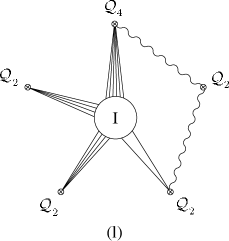
Figure 11: Diagrammatic representation of the non-perturbative Yang–Mills contributions to the correlation function $\langle{\cal Q}_{4}{\cal Q}_{2}{\cal Q}_{2}{\cal Q}_{2}{\cal Q}_{2}\rangle$. The notation is the same used in previous figures.

Writing the $SU(4)$ indices explicitly the correlation function (185) becomes

$$\hat{G}_{5} \!=\! \langle{\cal Q}^{[A_{1}B_{1}][C_{1}D_{1}][E_{1}F_{1}][G_{1}H_{1}]}(x_{1}){\cal Q}^{[A_{2}B_{2}][C_{2}D_{2}]}(x_{2})$$ (187)

$${\cal Q}^{[A_{3}B_{3}][C_{3}D_{3}]}(x_{3}){\cal Q}^{[A_{4}B_{4}][C_{4}D_{4}]}(x_{4}){\cal Q}^{[A_{5}B_{5}][C_{5}D_{5}]}(x_{5})\rangle\,,$$

where as in previous sections we use a hat to distinguish the Yang–Mills correlation function from the dual AdS amplitude to be considered in the following.

We will not compute the individual diagrams in detail since they are rather involved, but simply sketch how the generalisation of the perturbative result ought to work. The factorisation (7.3) was proved in [12] using classical supergravity and is therefore a leading order result in the $1/N$ expansion. We will also study the instanton effects only at leading order, which is $N^{1/2}$.

The diagrams in figure 11 can be organised in three groups of four characterised by the number of scalar contractions, $s=0,1,2$. Diagrams (a)-(d) form the first group ($s=0$), diagrams (e)-(h) the second group ($s=1$) and diagrams (i)-(l) the third group ($s=3$). The first four diagrams have no contractions and thus involve four $({\bar{\nu}}\nu)$ pairs. Recalling the normalisation of chiral primary operators in (54) and the general rules for the counting of powers of $N$ and $g_{{}_{\rm YM}}$ derived in section 3.2, we find that diagrams 11(a)-(d) are all of order

$$\left(\frac{N}{g_{{}_{\rm YM}}^{2}N}\right)^{4}\frac{N}{g_{{}_{\rm YM}}^{4}N^{2}}\>g_{{}_{\rm YM}}^{12}N\,N^{1/2}=N^{1/2}\,,$$ (188)

where the first two factors are the normalisations of the five operators and the remaining factors are those associated with the instanton measure and $({\bar{\nu}}\nu)$ insertions according to (46). Diagrams (a) and (b) can be argued to vanish after integration over the angular variables $\Omega^{AB}$ on the basis of group theory. In the case of (a) the operator ${\cal Q}_{4}$ soaks up all the ${\bar{\nu}}$ and $\nu$ modes. This means that they must be combined in the 105 of $SU(4)$ and thus the corresponding angular integral vanishes because it selects a singlet. In the case of diagram (b) it is easy to see that the two $(\bar{\nu}\nu)_{\bf 6}$ and one $(\bar{\nu}\nu)_{\bf 10}$ in the ${\cal Q}_{4}$ insertion must be combined to form a 126, which again means that the angular integral is zero because the remaining $({\bar{\nu}}\nu)$ bilinear is in the 10 and the product ${\bf 126}\times{\bf 10}$ does not contain the singlet. The other two diagrams, (c) and (d), are potentially non zero. The result for (c) is of the form

$$\hat{G}_{5}^{\rm(c)} \!=\! c_{\rm c}(N)\,{\rm e}^{2\pi i\tau}t_{\rm c}^{A_{1}B_{1}C_{1}D_{1}A_{2}B_{2}C_{2}D_{2}}\int\frac{d^{4}x_{0}d\rho}{\rho^{5}}\frac{\rho^{6}}{[(x_{1}-x_{0})^{2}+\rho^{2}]^{6}}(\zeta\zeta\zeta\zeta)^{E_{1}F_{1}G_{1}H_{1}}$$ (189)

$$\frac{\rho^{2}}{[(x_{2}-x_{0})^{2}+\rho^{2}]^{2}}\prod_{i=3}^{5}\frac{\rho^{4}}{[(x_{i}-x_{0})^{2}+\rho^{2}]^{4}}(\zeta\zeta\zeta\zeta)^{A_{i}B_{i}C_{i}D_{i}}+\cdots$$

where

$$c_{\rm c}(N)\sim N^{1/2}+O(N^{-1/2})$$ (190)

and the tensor $t_{\rm c}^{A_{1}B_{1}C_{1}D_{1}A_{2}B_{2}C_{2}D_{2}}$ is determined by the angular integration. In (189) we have ordered the insertion points clockwise starting from $x_{1}$ where ${\cal Q}_{4}$ is located and we have schematically indicated by $(\zeta\zeta\zeta\zeta)^{ABCD}$ the combination of superconformal modes entering in the operators ${\cal Q}_{4}$ and ${\cal Q}_{2}$ (see (63), (280) and (73)). The ellipsis stands for permutations corresponding to the other ways of distributing the zero modes with the fixed structure in figure 11(c).

The contribution of (d) takes the form

$$\hat{G}_{5}^{\rm(d)} \!=\! c_{\rm d}(N)\,{\rm e}^{2\pi i\tau}t_{\rm d}^{A_{1}B_{1}C_{1}D_{1}A_{2}B_{2}A_{3}B_{3}}\int\frac{d^{4}x_{0}d\rho}{\rho^{5}}\frac{\rho^{6}}{[(x_{1}-x_{0})^{2}+\rho^{2}]^{6}}(\zeta\zeta\zeta\zeta)^{E_{1}F_{1}G_{1}H_{1}}$$ (191)

$$\prod_{i=2}^{3}\frac{\rho^{3}}{[(x_{i}-x_{0})^{2}+\rho^{2}]^{3}}(\zeta\zeta)^{C_{i}D_{i}}\prod_{i=4}^{5}\frac{\rho^{4}}{[(x_{i}-x_{0})^{2}+\rho^{2}]^{4}}(\zeta\zeta\zeta\zeta)^{A_{i}B_{i}C_{i}D_{i}}+\cdots\,,$$

where the dots again stand for permutations and as in case (c) we have

$$c_{\rm d}(N)\sim N^{1/2}+O(N^{-1/2})\,.$$ (192)

Of the second set of four diagrams, which have one scalar contraction, only the first two are of the same order, $N^{1/2}$, as the previous ones and need to be taken into account. Diagrams (g) and (h) would be subleading, but actually they vanish after integration over the five sphere since the ${\bar{\nu}}$ and $\nu$ modes can not be combined to form a singlet. Diagrams (e) and (f) have two $(\bar{\nu}\nu)_{\bf 6}$ insertions and thus the counting of powers of $g_{{}_{\rm YM}}$ and $N$ for these contributions goes exactly as in (188). The evaluation of these two diagrams is rather lengthy and the result we get is of the form

$$\hat{G}_{5}^{\rm(e)}=c_{\rm e}(N)\,{\rm e}^{2\pi i\tau}\varepsilon^{A_{1}B_{1}C_{1}D_{1}}\int\frac{d^{4}x_{0}d\rho}{\rho^{5}}\frac{\rho^{6}}{[(x_{1}-x_{0})^{2}+\rho^{2}]^{6}}(\zeta\zeta\zeta\zeta)^{E_{1}F_{1}G_{1}H_{1}}$$

$$\varepsilon^{C_{2}D_{2}C_{3}D_{3}}\left[\frac{(\zeta\zeta\zeta\zeta)^{A_{2}B_{2}A_{3}B_{3}}}{(x_{2}-x_{3})^{2}}\prod_{i=2}^{3}\frac{\rho^{2}}{[x_{i}-x_{0})^{2}+\rho^{2}]^{2}}+(\zeta\zeta\zeta\zeta)^{A_{2}B_{2}A_{3}B_{3}}\prod_{i=2}^{3}\frac{\rho^{3}}{[x_{i}-x_{0})^{2}+\rho^{2}]^{3}}\right]$$

$$\prod_{i=4}^{5}\frac{\rho^{4}}{[(x_{i}-x_{0})^{2}+\rho^{2}]^{4}}(\zeta\zeta\zeta\zeta)^{A_{i}B_{i}C_{i}D_{i}}+\cdots\,,$$ (193)

for (e) and

$$\hat{G}_{5}^{\rm(f)} \!=\! c_{\rm f}(N)\,{\rm e}^{2\pi i\tau}\varepsilon^{A_{1}B_{1}C_{1}D_{1}}\int\frac{d^{4}x_{0}d\rho}{\rho^{5}}\,\varepsilon^{E_{1}F_{1}A_{2}B_{2}}\left[\frac{\rho^{5}}{[(x_{1}-x_{0})^{2}+\rho^{2}]^{5}}\frac{\rho^{3}\>(\zeta\zeta\zeta\zeta)^{G_{1}H_{1}C_{2}D_{2}}}{[(x_{2}-x_{0})^{2}+\rho^{2}]^{3}}\right.$$ (194)

$$\left.+\frac{1}{(x_{1}-x_{2})^{2}}\frac{\rho^{4}}{[(x_{1}-x_{0})^{2}+\rho^{2}]^{4}}\frac{\rho^{2}}{[(x_{2}-x_{0})^{2}+\rho^{2}]^{2}}(\zeta\zeta\zeta\zeta)^{G_{1}H_{1}C_{2}D_{2}}\right]$$

$$\prod_{i=4}^{5}\frac{\rho^{4}}{[(x_{i}-x_{0})^{2}+\rho^{2}]^{4}}(\zeta\zeta\zeta\zeta)^{A_{i}B_{i}C_{i}D_{i}}+\cdots\,,$$

for (f). In both (193) and (194) the dots stand for permutations and other contributions with the same structure corresponding to contractions between different pairs of scalars. As already observed both the coefficients $c_{\rm e}(N)$ and $c_{\rm f}(N)$ start at order $N^{1/2}$.

The remaining four diagrams have no $\nu$ and ${\bar{\nu}}$ insertions and so have no additional powers of $N$ associated with colour contractions in $({\bar{\nu}}\nu)$ bilinears. A counting of powers of $g_{{}_{\rm YM}}$ an $N$ for these diagrams gives

$$\left(\frac{N}{g_{{}_{\rm YM}}^{2}N}\right)^{4}\frac{N}{g_{{}_{\rm YM}}^{4}N^{2}}\>g_{{}_{\rm YM}}^{12}\,N^{1/2}=N^{-1/2}\,.$$ (195)

In diagram (i) we get an additional power of $N$ from the double scalar contraction, hence this is the only contribution that we need to take into account at leading order, $N^{1/2}$. The remaining diagrams (j), (k) and (l) are subleading and we will not examine them here. In the previous diagrams the only term in the propagator which gave a non-vanishing contribution was the one in the first line of (53), this is also true for (i) at leading order. The other terms only give rise to subleading contributions. The order $N^{1/2}$ part of (i) reads

$$\hat{G}_{5}^{\rm(i)} \!=\! c_{\rm i}(N)\,{\rm e}^{2\pi i\tau}\varepsilon^{E_{1}F_{1}A_{2}B_{2}}\varepsilon^{G_{1}H_{1}C_{2}D_{2}}\int\frac{d^{4}x_{0}d\rho}{\rho^{5}}\,\left[\frac{1}{(x_{1}-x_{2})^{4}}\frac{\rho^{4}\>(\zeta\zeta\zeta\zeta)^{A_{1}B_{1}C_{1}D_{1}}}{[x_{1}-x_{0})^{2}+\rho^{2}]^{4}}\right.$$ (196)

$$\left.+\frac{1}{(x_{1}-x_{2})^{2}}\frac{\rho^{5}}{[x_{1}-x_{0})^{2}+\rho^{2}]^{5}}\frac{\rho}{[(x_{1}-x_{0})^{2}+\rho^{2}]}(\zeta\zeta\zeta\zeta)^{E_{1}F_{1}G_{1}H_{1}}\right]$$

$$\prod_{i=2}^{5}\frac{\rho^{4}}{[x_{i}-x_{0})^{2}+\rho^{2}]^{4}}(\zeta\zeta\zeta\zeta)^{A_{i}B_{i}C_{i}D_{i}}+\cdots\,.$$

Notice that this expression indeed contains a term with the factorised structure $\langle{\cal Q}_{2}(x_{1}){\cal Q}_{2}(x_{2})\rangle\langle{\cal Q}_{2}(x_{1}){\cal Q}_{2}(x_{1}){\cal Q}_{2}(x_{1}){\cal Q}_{2}(x_{1})\rangle_{\rm inst}$, where the second factor is the instanton contribution to the minimal four-point function of chiral primaries of dimension 2, i.e.

$$\frac{\varepsilon^{E_{1}F_{1}A_{2}B_{2}}\varepsilon^{G_{1}H_{1}C_{2}D_{2}}}{(x_{1}-x_{2})^{4}}\>N^{1/2}\,{\rm e}^{2\pi i\tau}\int\frac{d^{4}x_{0}d\rho}{\rho^{5}}\prod_{\begin{array}[]{c}\scriptstyle i=1\\ \raisebox{15.0pt}{$\scriptstyle i\neq 2$}\end{array}}^{5}\frac{\rho^{4}}{[x_{i}-x_{0})^{2}+\rho^{2}]^{4}}(\zeta\zeta\zeta\zeta)^{A_{i}B_{i}C_{i}D_{i}}\,.\vspace*{-20pt}$$ (197)

In conclusion, our results are consistent with the possibility that the factorisation property (7.3) of the near-extremal five-point function remains valid when instanton corrections are included. However, for this to happen several contributions would have to cancel. The contributions of (189), (191), (193), (194) and the second term in (196), which do not individually vanish, do not possess the factorised structure of (7.3) but their sum might vanish when the precise coefficients are evaluated.

We now discuss the AdS processes contributing to the dual amplitude at leading order. All the relevant $AdS_{5}$ Witten diagrams involve a ${\cal R}^{4}$ D-instanton induced vertex and can be represented as in figure 12. All the lines in figures represent scalar fields dual to the chiral primary operators ${\cal Q}_{\ell}$. As in previous sections we denote this field and its Kaluza–Klein excited modes by $Q$. In the figure we have indicated the dimension of the associated field next to each line.

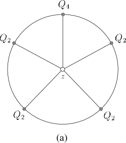
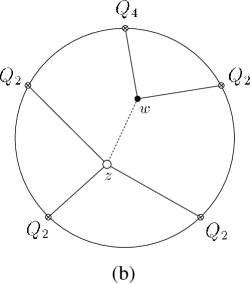
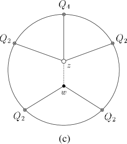
Figure 12: Diagrammatic representation of the AdS amplitudes contributing to the process dual to the correlation function $\langle{\cal Q}_{4}{\cal Q}_{2}{\cal Q}_{2}{\cal Q}_{2}{\cal Q}_{2}\rangle$.

There is an obvious contribution which comes from a contact diagram obtained expanding the ${\cal R}^{4}$ coupling. This is represented in figure 12(a) and the resulting amplitude takes the form

$$G^{5}_{\rm a}=c_{\rm a}(\tau,\bar{\tau},N)\int\frac{d^{5}z}{z_{0}^{5}}\,\frac{\partial^{8}}{\partial z^{8}}\left[K_{4}(z;x_{1})\prod_{i=2}^{5}K_{2}(z;x_{i})\right]\,,$$ (198)

where we have indicated schematically the eight derivatives entering the ${\cal R}^{4}$ coupling that act on the bulk-to-boundary propagators. The coefficient $c_{\rm a}(\tau,\bar{\tau},N)$ encodes the dependence on $N$ and the coupling which are those obtained from the ${\cal R}^{4}$ interaction at order $({\alpha^{\prime}})^{-1}$

$$c_{\rm a}(\tau,\bar{\tau},N)=c_{\rm a}\,{\rm e}^{2\pi i\tau}\left(N^{1/2}+O(N^{-1/2})\right)\,.$$ (199)

The second type of contribution corresponds to exchange diagrams with four lines coming out of a ${\cal R}^{4}$ vertex and an additional cubic interaction, see figure 12(b) and (c). There are four possible contributions of this type corresponding to the fact that the bulk-to-bulk lines in these figures can each be dual to an operator of dimension 2 or 4. In the case of figure 12(b) when the intermediate line is a dimension 2 field, the vertex in $w$ is extremal and the result reduces to

$$G^{5}_{\rm b}=c_{\rm b}(\tau,\bar{\tau},N)\frac{1}{(x_{1}-x_{2})^{4}}\int\frac{d^{5}z}{z_{0}^{5}}\,\frac{\partial^{8}}{\partial z^{8}}\prod_{\begin{array}[]{c}\scriptstyle i=1\\ \raisebox{15.0pt}{$\scriptstyle i\neq 2$}\end{array}}^{5}K_{2}(z;x_{i})\,.\vspace*{-20pt}$$ (200)

The contribution in which the intermediate state has dimension 4 can be computed using the formulae derived in [41]. However, it is expected to vanish, because the D-instanton vertex in $z$ was argued in [38] to be zero to reproduce the non-renormalisation of next-to-extremal correlation functions. For the same reason the process of figure 12(c) in which the intermediate state is dual to a dimension 2 operator also vanishes. The remaining possibility is the exchange of a dimension 4 operator. In this case the vertex in $w$ is extremal and the result is of the form

$$G^{5}_{\rm c}=c_{\rm c}(\tau,\bar{\tau},N)\int\frac{d^{5}z}{z_{0}^{5}}\,\frac{\partial^{8}}{\partial z^{8}}\left[K_{4}(z;x_{1})\prod_{i=2}^{5}K_{2}(z;x_{i})\right]\,,$$ (201)

i.e. the same as (198). For the two contributions in (200) and (201) we find again

$$c_{\rm b,c}(\tau,\bar{\tau},N)=c_{\rm b,c}\,{\rm e}^{2\pi i\tau}\left(N^{1/2}+O(N^{-1/2})\right)\,.$$ (202)

The AdS result therefore has potentially two contribution. One is a contact term resulting from the sum of (198) and (201) and the other, (200), has the factorised structure found in perturbation theory. It is striking to conjecture that the first two contributions should cancel leaving no contact amplitude and a total amplitude with the factorised form.

To summarise, our calculations are compatible with the possibility that the partial non-renormalisation of the near-extremal five-point function (187) is valid beyond perturbation theory. Although we have only carried out a qualitative analysis which does not allow us to check all the required cancellations and give a complete proof, it is impressive that it is a possibility.

7.4 Anti-instanton contributions

We conclude this section with a comment about anti-instanton contributions to correlation functions like those considered in [5, 6], which are minimal in the instanton ($K=+1$) background. Equivalently, we can study instanton contributions to correlation functions with insertions of the fields conjugate to those in (63) that we have considered up to this point. These fields contain more fermionic zero-modes in the background of an instanton and thus give rise to non-minimal correlation functions. The simplest cases to analyse are again those with the maximal number of fermionic insertions. We can consider for instance

$$\hat{G}_{\hat{\bar{\Lambda}}^{16}}=\langle\hat{\bar{\Lambda}}_{A_{1}}^{{\dot{\alpha}}_{1}}(x_{1})\ldots\hat{\bar{\Lambda}}_{A_{16}}^{{\dot{\alpha}}_{16}}(x_{16})\rangle\,,$$ (203)

where $\hat{\bar{\Lambda}}_{A}^{{\dot{\alpha}}}$ is the operator

$$\hat{\bar{\Lambda}}_{A}^{{\dot{\alpha}}}={\rm Tr}\left({\bar{\sigma}}^{{\dot{\alpha}}}_{mn\>{\dot{\beta}}}F^{mn}\bar{\lambda}^{\dot{\beta}}_{A}\right)\,,$$ (204)

transforming in the representation ${\bf 4^{*}}$ of $SU(4)$.

In the instanton background $F^{+}_{mn}$, which appears in (204), contains at least four zero-modes and $\bar{\lambda}^{\dot{\beta}}_{A}$ three, so there are seven fermionic modes for each insertion in (203), for a total of 112. Of these, sixteen must be superconformal modes that produce a non-vanishing result, which leaves 48 $\bar{\nu}\nu$ bilinears, which we expect to be only of the $(\bar{\nu}\nu)_{\bf 10}$ type. According to the general formulae of section 3.2 we therefore expect a leading $g_{{}_{\rm YM}}$ and $N$ dependence of the type

$$\hat{G}_{\hat{\bar{\Lambda}}^{16}}\sim N^{1/2}g_{{}_{\rm YM}}^{24}{\rm e}^{2\pi i\tau}\,,$$ (205)

where the powers of $g_{{}_{\rm YM}}$ are obtained by combining a factor of $g_{{}_{\rm YM}}^{-32}$ from the normalisation of the operators (see (54)) and factors of $g_{{}_{\rm YM}}^{48}$ and $g_{{}_{\rm YM}}^{8}$ from the $(\bar{\nu}\nu)_{\bf 10}$ insertions and the instanton measure respectively.

The dependence on the parameters in (205) agrees with the prediction of supergravity. Indeed the vertex $\bar{\Lambda}^{16}$, which generates the amplitude dual to (203), appears in the type IIB effective action at order ${\alpha^{\prime}}^{-1}$ multiplied by the modular form $f_{1}^{(-12,12)}(\tau,\bar{\tau})$, which has a leading instanton contribution starting as $\tau_{2}^{-12}=g_{\rm s}^{12}$.

In general, correlation functions such as (203) with insertions of operators conjugate to those entering minimal correlation functions are much more involved, because they are suppressed by many powers of the coupling $g_{{}_{\rm YM}}$, which allows for the possibility of complicated contributions with scalar contractions at leading non-vanishing order. A detailed analysis of these processes is outside the scope of this paper.

8 Discussion

In this paper we have studied the structure of a variety of correlation functions of gauge invariant composite operators in ${\cal N}=4$ $SU(N)$ Yang–Mills theory in a one-instanton background at large $N$ and at leading order in the coupling constant, $g_{{}_{\rm YM}}$. One of the main motivations was to understand to what extent the $1/N$ expansion of instanton-induced contributions to correlation functions in the ${\cal N}=4$ supersymmetric Yang–Mills theory encodes information about higher-derivative terms in the type IIB effective action via the AdS/CFT correspondence. Another motivation was to understand instanton effects for processes involving composite Yang–Mills operators that are dual to Kaluza–Klein excitations of the supergravity fields.

The calculation of Yang–Mills correlation functions that we have considered includes the contributions of the fermionic moduli, $\nu^{A}$ and $\bar{\nu}^{A}$, that are superpartners of the gauge rotations that describe the embedding of $SU(2)$ in $SU(N)$. Within the context of the AdS/CFT conjecture such modes are essential in accounting for the Kaluza–Klein excitations of the type IIB supergravity fields on the five-sphere in the presence of a single D-instanton. They are also essential in accounting for higher-order interactions in the effective type IIB string theory action in the $AdS_{5}\times S^{5}$ background. A prime example of this is the ${\alpha^{\prime}}G^{4}\Lambda^{16}$ interaction. This corresponds to a contribution to the $\langle\hat{\Lambda}^{16}{\cal E}^{4}\rangle$ of order $N^{-1/2}$, which is suppressed by a power of $1/N$ relative to the dominant instanton contributions. However, we found that the explicit Yang–Mills calculation gives a leading term of order $N^{1/2}$. In order to explain this it was important to appreciate that the $AdS_{5}\times S^{5}$ contributions are not entirely given by a single instanton-induced interaction. It is essential to include certain tree diagrams which have one induced D-instanton vertex and classical interactions at the other vertices. For example, the tree diagram for the $\langle\Lambda^{16}G^{4}\rangle$ amplitude has two propagators for a $\tau_{20^{\prime}}$, which is a Kaluza–Klein excitation of the dilaton. The coupling of these fields to the external $G$’s arises from the $\bar{\tau}\,G^{2}$ coupling of classical type IIB supergravity. This generates a new kind of instantonic contact interaction, thereby explaining the $N^{1/2}$ contribution to the $\langle\hat{\Lambda}^{16}{\cal E}^{4}\rangle$ correlation function. Since the Kaluza–Klein excitations are absent from the consistently truncated five-dimensional gauged $N=8$ supergravity, we would expect such contact terms to arise directly as D-instanton contact terms in the dimensionally reduced theory.

In the simplest instanton-induced correlation functions all of the fields in the composite operators are replaced by their ‘classical’ profiles, which include the fermionic zero modes. More generally, in the examples that we studied, even at leading order in $g_{{}_{\rm YM}}$, the effect of quantum fluctuations which give rise to propagators in the instanton background needs to be taken into account. In practice, the only propagator we needed to consider is the scalar propagator $\langle\varphi^{a}(x_{1})\varphi^{b}(x_{2})\rangle_{\rm inst}$. Although the complete expression for this propagator (53) looks complicated, its insertion in correlation functions of gauge-invariant composite operators gives rise to simple spatial structures. The combination of the terms in (53) produces contributions to Yang–Mills correlation functions which are found to reproduce the supergravity amplitudes with D-instanton induced vertices and additional tree-level interactions described above. Contributions of this type arose, for example, in determining the form of the $\langle\hat{\Lambda}^{16}{\cal Q}_{2}^{2}\rangle$ correlation function. In this example, that we discussed in detail, the combination of different effects on both sides of the correspondence is required to reconcile the results with the AdS/CFT duality.

These considerations constitute a small step towards unraveling the systematics of the $N$-dependence of instanton effects. We have restricted our analysis to the one-instanton sector. On the other hand, as shown in [6], the large-$N$ limit simplifies drastically the study of multi-instantons and their comparison with D-instanton effects in type IIB string theory. It would be interesting to extend the results of this paper to the generic $K$-instanton sector at large $N$. This would generalise the work of [6] to the class of non-minimal correlation functions and allow to investigate the large-$N$ limit of the $K$-instanton contributions beyond leading order. This program involves systematically expanding the instanton measure as well as the expressions for the composite operators. Both of these tasks are formidable and still incomplete.

There are other obvious areas in which the fermionic moduli $\nu^{A}$ and $\bar{\nu}^{A}$ and the other effects discussed in this paper should play an essential rôle. One of these is the instanton contribution to the BPS Wilson loop [47] in ${\cal N}=4$ supersymmetric $SU(N)$ Yang–Mills theory. The generalization of the arguments for the $SU(2)$ case of [48] to the $SU(N)$ case requires the inclusion of the additional $\nu$ and ${\bar{\nu}}$ modes as well as the contribution of contractions. In particular, in the $N\to\infty$ limit the sum of these additional contributions becomes an infinite series which could exponentiate and, combined with the perturbative result, give rise to an expression that transforms covariantly under S-duality. Likewise, the BMN limit [49] of superconformal Yang–Mills theory involves an infinite boost along a great circle of the five-sphere which is dominated by highly excited angular momentum states. This will involve the $\nu^{A}$ and $\bar{\nu}^{A}$ moduli in an essential manner. D-instanton configurations in a plane-wave background have been constructed [50], suggesting that instanton effects should also play a rôle in this limit. An interesting class of observables in the ${\cal N}=4$ supersymmetric Yang–Mills theory comprises correlation functions which are not protected by symmetry from receiving quantum corrections, but display ‘partial non-renormalisation properties’. Examples of this type of quantity are the near-extremal correlation functions, such as the one discussed in section 7.3. The partial non-renormalisation properties of four-point functions of chiral primary operators have been recently studied in the case of operators of dimension $\Delta=3$ [51, 52] and it was found that all these four-point correlation functions, as in the case of dimension two operators, can be expressed in terms of a unique function of two conformally invariant cross ratios. The proof that this property is still valid when instanton corrections are included would require the application of the techniques discussed in this paper. Finally, the Konishi multiplet in ${\cal N}=4$ super Yang–Mills is known to possess some unexpected non-perturbative non-renormalisation properties [29], namely its two-, three- and four-point functions do not receive instanton corrections. Higher-point functions with insertions of operators in the Konishi multiplet are non-minimal in the sense discussed here and appear to have non-vanishing instanton contributions [53].

Appendix A Conventions and useful relations

In this appendix we will summarize a few useful identities associated with $SO(4)$ and $SO(6)$ spinors.

The four-dimensional sigma matrices are defined by

$$\sigma^{m}=(\mathbbm{1},i\tau^{i})\,,\qquad\bar{\sigma}^{m}=(\mathbbm{1},-i\tau^{i})\,,$$ (206)

where $\tau^{i}$ are the Pauli matrices. The self-dual tensor $\sigma^{mn}{}_{\beta}{}^{\gamma}$ is defined by

$$\sigma^{mn}{}_{\beta}{}^{\gamma}=\frac{1}{4}(\sigma^{m}{}_{\beta{\dot{\alpha}}}{\bar{\sigma}}^{n{\dot{\alpha}}\gamma}-\sigma^{n}{}_{\beta{\dot{\alpha}}}{\bar{\sigma}}^{m{\dot{\alpha}}\gamma})\,.$$ (207)

The $SO(6)$ sigma matrices are defined by

$$\Sigma^{a}_{AB}=(\eta^{i}_{AB},i\bar{\eta}^{i}_{AB})\,,\qquad\bar{\Sigma}_{a}^{AB}=(-\eta_{i}^{AB},i\bar{\eta}^{AB}_{i})\,~{}~{}{\rm with}~{}a=1,\dots,6$$ (208)

and the ’t Hooft symbols, for $i=1,2,3$, are

$$\eta^{i}_{AB}=\bar{\eta}^{i}_{AB}=\varepsilon_{iAB}\qquad A,B=1,2,3\,,$$

$$\eta^{i}_{A4}=\bar{\eta}^{i}_{4A}=\delta^{i}_{A}\,,$$

$$\eta^{i}_{AB}=-\eta^{i}_{BA}\,,\qquad\bar{\eta}^{i}_{AB}=-\bar{\eta}^{i}_{BA}\,.$$ (209)

The following properties of the ’t Hooft symbols are of use,

$$\eta^{i}_{mn}\sigma^{mn}_{\,{\alpha}}{}^{\beta}=2i\tau^{i}_{\,{\alpha}}{}^{\beta}\,,\qquad\bar{\eta}^{i}_{mn}\bar{\sigma}^{mn}_{\,{\dot{\alpha}}}{}^{\dot{\beta}}=2i\tau^{i}_{\,{\dot{\alpha}}}{}^{\dot{\beta}}\,.$$ (210)

$$\eta^{i}_{mn}\tau^{i}_{\,{\alpha}}{}^{\beta}=-2i\sigma^{mn}_{\,{\alpha}}{}^{\beta}\,,\qquad\bar{\eta}^{i}_{mn}\tau^{i}_{\,{\dot{\alpha}}}{}^{\dot{\beta}}=-2i\bar{\sigma}^{mn}_{\,{\dot{\alpha}}}{}^{{\dot{\beta}}}\,.$$ (211)

$${\rm tr}\left(\sigma_{mn}\tau^{i}\right)=i\eta^{i}_{mn}\,,\qquad{\rm tr}\left(\bar{\sigma}_{mn}\tau^{i}\right)=i\bar{\eta}^{i}_{mn}\,.$$ (212)

The $SO(6)$ sigma matrices satisfy the following relations

$$\varepsilon^{ABCD}\Sigma^{a}_{CD}=-2{\bar{\Sigma}}^{a\,AB}\>,\qquad\varepsilon_{ABCD}{\bar{\Sigma}}^{a\,CD}=-2\Sigma^{a}_{AB}\,.$$ (213)

$$\frac{1}{2}\left(\Sigma^{a}_{AC}{\bar{\Sigma}}^{b\,CB}+\Sigma^{b}_{AC}{\bar{\Sigma}}^{a\,CB}\right)=\delta^{ab}\delta_{A}^{B}\,,$$ (214)

$$\Sigma^{a}_{AC}{\bar{\Sigma}}^{b\,CB}=\delta^{ab}\delta_{A}^{B}+\Sigma_{A}^{ab\,B}$$ (215)

where $\Sigma_{A}^{ab\,B}=\frac{1}{2}\left(\Sigma^{a\,AC}{\bar{\Sigma}}^{b}_{CB}-\Sigma^{b\,AC}{\bar{\Sigma}}^{a}_{CB}\right)$. The following identities are also of use,

$${\bar{\Sigma}}^{a\,AB}\Sigma^{a}_{CD}=2(\delta^{A}_{D}\delta^{B}_{C}-\delta^{A}_{C}\delta^{B}_{D})\,.$$ (216)

$$(\Sigma^{a}{\bar{\Sigma}}^{a})^{A}_{B}=6\delta^{A}_{B}\,.$$ (217)

$$\Sigma^{a}_{AB}\Sigma^{a}_{CD}=2\varepsilon_{ABCD}\,.$$ (218)

$$\Sigma_{A}^{ab\,B}\Sigma_{B}^{cd\,A}=-4\left(\delta^{ac}\delta^{bd}-\delta^{ad}\delta^{bc}\right)\,.$$ (219)

$$\chi_{AB}={1\over\sqrt{8}}\Sigma^{a}_{AB}\chi_{a}\,,\qquad\chi_{a}={1\over\sqrt{2}}{\bar{\Sigma}}_{a}^{AB}\chi_{BA}\,.$$ (220)

$${\rm tr}({\bar{\Sigma}}^{a}\Sigma^{b}{\bar{\Sigma}}^{c}\Sigma^{d})=4\delta^{ab}\delta^{cd}-4\delta^{ac}\delta^{bd}+4\delta^{ad}\delta^{bc}\,.$$ (221)

Appendix B Summary of ADHM for ${\cal N}=4$ theory

In this appendix we include for completeness a few formulae used in the description of multi-instanton configurations in the ADHM formalism. The discussion is by no means complete, we refer the reader for instance to [18] for a very comprehensive review.

The classical $K$-instanton solution is defined in terms of a $[N+2K]\times[2K]$ dimensional matrix $\Delta_{ai}{}^{{\alpha};j{\dot{\alpha}}}$ which is a linear function of the space-time coordinate $x_{m}$,

$$\Delta_{ui{\alpha};}{}^{j}{}_{{\dot{\alpha}}}=a_{ui{\alpha};}{}^{j}{}_{{\dot{\alpha}}}+b_{ui{\alpha};}{}^{j\beta}\,x_{\beta{\dot{\alpha}}}\,,$$ (222)

and its conjugate,

$$\bar{\Delta}_{i}{}^{{\dot{\alpha}};j{\alpha}}=\bar{a}_{i}{}^{{\dot{\alpha}};j{\alpha}}+x^{{\dot{\alpha}}\beta}\,\bar{b}_{i\beta;}{}^{uj{\alpha}}$$ (223)

(we use latin letters from the mid of the alphabet, $i,j,k,...=1,...K$, to denote instanton indices). The ADHM gauge field is written in the form

$$(A_{m})_{u;}{}^{v}={\bar{U}}_{u;}{}^{ri{\alpha}}\partial_{m}U_{ri{\alpha};}{}^{v}\,,$$ (224)

where the complex $[N]\times[N+2K]$ matrix $U(x)$ and its hermitian conjugate ${\bar{U}}(x)$ satisfy

$${\bar{U}}_{u;}{}^{ri{\alpha}}U_{ri{\alpha};}{}^{v}=\delta_{u}{}^{v}\,,$$ (225)

$${\bar{\Delta}}_{i}{}^{{\dot{\alpha}};rj\beta}U_{rj\beta;}{}^{v}=0\,,\qquad{\bar{U}}_{u;}{}^{ri{\alpha}}\Delta_{ri{\alpha};}{}^{j}{}_{\dot{\alpha}}=0\,.$$ (226)

Equation (224) gives a gauge configuration with self-dual field strength provided the matrices $\Delta$ and ${\bar{\Delta}}$ satisfy

$${\bar{\Delta}}_{i}{}^{{\dot{\alpha}};rk\beta}\Delta_{rk\beta;}{}^{j}{}_{\dot{\beta}}=\delta^{\dot{\alpha}}{}_{\dot{\beta}}\left(f^{-1}\right)_{i}{}^{j}\,,$$ (227)

where $f(x)$ is an arbitrary ($x$-dependent) $[K]\times[K]$ hermitian matrix. From this relation and the definitions (222) and (223) it follows that the coefficients $a$ and $b$ satisfy the bosonic ADHM constraints

$$\bar{a}_{i}{}^{{\dot{\alpha}}}{}^{;uk{\alpha}}\,a_{uk{\alpha};}{}^{j}{}_{{\dot{\beta}}}={{1\over 2}}(\bar{a}a)_{i}{}^{k}\,\delta^{\dot{\alpha}}_{\dot{\beta}}\,,$$ (228)

$$\bar{a}_{ui}{}^{{\dot{\alpha}};j{\alpha}}\,b_{uj{\alpha};k}{}^{\beta}=\epsilon^{\beta\gamma}\,\epsilon^{{\dot{\alpha}}{\dot{\beta}}}\,\bar{b}_{i\gamma;}{}^{uj{\alpha}}\,a_{uj{\alpha};}{}^{k}{}_{{\dot{\beta}}}\,,$$ (229)

$$\bar{b}_{i\beta;}^{uk{\alpha}}\,b_{uk{\alpha};}{}^{j\gamma}={1\over 2}(\bar{b}b)_{i}{}^{j}\,\delta_{\beta}^{\gamma}\,.$$ (230)

A choice of special frame allows to put the bosonic parameters in the form

$$b_{ui{\alpha};}{}^{j\beta}=\left(\begin{array}[]{c}0_{u;}{}^{j\beta}\\ \delta_{i}{}^{j}\,\delta_{\alpha}{}^{\beta}\end{array}\right)\,,\qquad\bar{b}_{i{\alpha};}{}^{uj\beta}=\left(\begin{array}[]{c}0_{i{\alpha};}{}^{u}\\ \delta_{i}{}^{j}\,\delta_{\alpha}{}^{\beta}\end{array}\right)\,,$$ (231)

$$a_{ui{\alpha};}{}^{j}{}_{{\dot{\alpha}}}=\left(\begin{array}[]{c}w_{u;}{}^{j}{}_{{\dot{\alpha}}}\\ ({a^{\prime}}_{{\alpha}{\dot{\alpha}}})_{i}{}^{j}\end{array}\right)\,,\qquad\bar{a}_{i}{}^{{\dot{\alpha}};uj{\alpha}}=\left(\bar{w}_{i}{}^{{\dot{\alpha}};u}\,,(\bar{a^{\prime}}^{{\dot{\alpha}}{\alpha}})_{i}{}^{j}\right)\,,$$ (232)

where ${a^{\prime}}_{{\alpha}{\dot{\alpha}}}=\sigma_{{\alpha}{\dot{\alpha}}}^{m}\,{a^{\prime}}_{m}$ and the components satisfy the matrix constraints

$${\rm tr}_{2}({\tau^{c}}\,\bar{a}a)=0\,,\qquad{a^{\prime}}_{n}^{\dagger}={a^{\prime}}_{n}\,.$$ (233)

Similarly, the fermionic variables enter as $[N+2K]\times[K]$ grassmann valued matrices, ${\cal M}$ and $\bar{\cal M}$, that satisfy the ADHM constraints

$$\bar{\cal M}_{i;}^{A\,uj{\alpha}}\,a_{uj{\alpha};}{}^{k}{}_{{\dot{\alpha}}}=-\epsilon_{{\dot{\alpha}}{\dot{\beta}}}\,\bar{a}_{i}{}^{{\dot{\beta}};uj{\alpha}}\,{\cal M}_{uj{\alpha};}{}^{k},\qquad\bar{\cal M}^{A}_{i;}{}^{uj{\alpha}}\,b_{uj{\alpha};}{}^{k\beta}=\epsilon^{\beta\gamma}\,\bar{b}_{i\gamma;}{}^{uj{\alpha}}\,{\cal M}_{uj{\alpha};}{}^{k}\,,$$ (234)

Parametrising the fermionic matrices by

$${\cal M}^{A}_{ui{\alpha};}{}^{j}=\left(\begin{array}[]{c}\nu^{A\,}_{u;}{}^{j}+w_{u;}{}^{k{\dot{\alpha}}}\,{\bar{\xi}}^{A}_{{\dot{\alpha}}k;}{}^{j}\\ {{\cal M}^{\prime}}^{A}_{i{\alpha};}{}^{j}\end{array}\right)\equiv\left(\begin{array}[]{c}\mu^{A}_{u;}{}^{j}\\ {{\cal M}^{\prime}}^{A}_{i{\alpha};}{}^{j}\end{array}\right)\,,$$ (235)

$$\bar{\cal M}^{A\,}_{i;}{}^{uj{\alpha}}=\left(\bar{\nu}^{A}_{i;}{}^{u}+\bar{\tilde{\xi}}^{A}_{{\dot{\alpha}}i;}{}^{k}\,\bar{w}^{k{\dot{\alpha}};u}\,,\>{{\cal M}^{\prime}}^{A{\alpha}}_{\>i;}{}^{j}\right)\equiv\left(\bar{\mu}^{A}_{i;}{}^{u}\,,\>\bar{{\cal M}}^{\prime A}_{i;}{}^{\,j{\alpha}}\right)\,.$$ (236)

The ADHM conditions imply that

$$\bar{w}^{{\dot{\alpha}}}_{k;}{}^{u}\,\nu^{A}_{u;}{}^{i}=0,\qquad\bar{\nu}^{A}_{i;}{}^{u}\,w_{u;}{}^{k{\dot{\alpha}}}=0,\qquad\bar{w}^{\dot{\alpha}}_{i;}{}^{u}\,w_{u;{\dot{\beta}}}{}^{j}=W^{\dot{\alpha}}{}_{{\dot{\beta}}i;}{}^{j}\,,$$ (237)

$$\bar{\cal M}^{\prime A\ {\alpha}}_{i;}{}^{j}\,\delta_{j}{}^{k}\,\delta_{\alpha}{}^{\beta}=\epsilon^{\beta\gamma}\,\delta_{i}{}^{j}\,\delta_{\gamma}{}^{{\alpha}}\,{{\cal M}^{\prime}}^{A}_{j{\alpha};}{}^{k}\,.$$ (238)

The latter equation implies

$$\bar{\cal M}^{\prime A\ \beta}_{i;}{}^{k}=\epsilon^{\beta{\alpha}}\,{{\cal M}^{\prime}}^{A}_{i{\alpha};}{}^{k}\,.$$ (239)

The gauge invariant bosonic variables are contained in

$$W^{\dot{\beta}}{}_{{\dot{\alpha}}\,i;}{}^{j}=\bar{w}^{\dot{\beta}}{}_{i;}{}^{u}\,w_{u;{\dot{\alpha}}}{}^{j}\,,$$ (240)

which can be written as

$$(W^{\dot{\beta}}{}_{{\dot{\alpha}}})_{i}{}^{j}={1\over 2}\,(W^{0})_{i}{}^{j}\,\delta_{\dot{\alpha}}{}^{{\dot{\beta}}}+{1\over 2}(W^{c})_{i}{}^{j}\,{\tau^{c}}^{{\dot{\beta}}}{}_{\dot{\alpha}}\,.$$ (241)

Inverting this expression we have

$$(W^{0})_{i}{}^{j}={\rm tr}_{2}\,W_{i}{}^{j}=(W^{\dot{\alpha}}{}_{{\dot{\alpha}}})_{i}{}^{j}\,,\qquad(W^{c})_{i}{}^{j}={\rm tr}_{2}\,({\tau^{c}}W_{i}{}^{j})=\tau^{c\,{\dot{\beta}}}{}_{\dot{\alpha}}\,(W^{\dot{\alpha}}{}_{{\dot{\beta}}})_{i}{}^{j}\,.$$ (242)

The ADHM constraints can then be expressed as

$$W^{c}_{i}{}^{j}+[{a^{\prime}}_{m},{a^{\prime}}_{n}]_{i}{}^{j}\,{\tau^{c}}_{\dot{\alpha}}^{\ {\dot{\beta}}}\,\bar{\sigma}^{mn\ {\dot{\alpha}}}_{\ \ {\dot{\beta}}}=W^{c}_{i}{}^{j}-i[{a^{\prime}}_{m},{a^{\prime}}_{n}]_{i}{}^{j}\,\bar{\eta}^{c}_{mn}=0$$ (243)

(where $\bar{\eta}$ is the conjugate ’t Hooft symbol) and

$$\bar{\tilde{\xi}}^{A}_{{\dot{\alpha}}i}{}^{j}\,W^{\dot{\alpha}}_{\ {\dot{\beta}}\,j}{}^{k}+\epsilon_{{\dot{\beta}}{\dot{\gamma}}}\,W^{\dot{\gamma}}_{\ {\dot{\alpha}}\,i}{}^{j}\,{\bar{\xi}}^{{\dot{\alpha}}A}_{j}{}^{k}+\left[{{\cal M}^{\prime}}^{A{\alpha}},{a^{\prime}}_{{\alpha}{\dot{\beta}}}\right]_{i}{}^{k}=0\,.$$ (244)

Appendix C Component fields in the one-instanton background

In this appendix we summarise the expressions for the elementary fields in the ${\cal N}=4$ SYM multiplet in terms of the ADHM variables, in particular we give explicit formulae in the one-instanton sector. All the fields in the multiplet are in the adjoint representation of the gauge group $SU(N)$ and can be represented as $[N]\times[N]$ matrices.

The (self-dual part of the) gauge field strength $F^{-}_{mn}$ in the instanton background follows from the construction of the gauge field $A_{m}$ in the previous section. The result is

$$\left(F^{mn}\right)_{u;}{}^{v}={\bar{U}}_{u;}{}^{ri{\alpha}}b_{ri{\alpha};}{}^{j\beta}\sigma^{mn}{}_{\beta}{}^{\gamma}f_{j;}{}^{k}{\bar{b}}_{k\gamma;}{}^{sl\delta}U_{sl\delta;}{}^{v}\,.$$ (245)

In the semiclassical approximation the Weyl fermions $\lambda^{A}_{\alpha}$ are replaced by the solutions to the zero-eigenvalue Dirac equation in the instanton background

$$\,{\raisebox{1.0pt}{$/$}D}\lambda^{A}_{\alpha}=0\,.$$ (246)

In terms of the ADHM variables the classical field $\lambda^{A}_{\alpha}$ is

$$\left(\lambda^{A}_{\alpha}\right)_{u;}{}^{v}={\bar{U}}_{u;}{}^{ri\beta}\left({\cal M}^{A}_{ri\beta;}{}^{j}f_{j;}{}^{k}{\bar{b}}_{k{\alpha};}{}^{sl\gamma}-\varepsilon_{{\alpha}\delta}b_{ri\beta;}{}^{j\delta}f_{j;}{}^{k}{\bar{\cal M}}^{A}_{k;}{}^{sl\gamma}\right)U_{sl\gamma;}{}^{v}$$ (247)

and it can be checked that it satisfies (246).

Analogously the scalar fields $\varphi^{AB}$ are replaced by the solution to their equation of motion in the instanton background at leading order in the Yang–Mills coupling

$$D^{2}\varphi^{AB}=\frac{i}{\sqrt{2}}[\lambda^{A},\lambda^{B}]\,.$$ (248)

The solution was constructed in [46]. In the ${\cal N}=4$ SYM theory in the superconformal phase of interest here the solution can be written in the form

$$i\varphi^{AB} = {1\over 2}{\bar{U}}_{u;}{}^{ri{\alpha}}\left({\cal M}^{B}_{ri{\alpha};}{}^{j}f_{j;}{}^{k}{\bar{\cal M}}^{A}_{k;}{}^{sl\beta}-{\cal M}^{A}_{ri{\alpha};}{}^{j}f_{j;}{}^{k}{\bar{\cal M}}^{B}_{k;}{}^{sl\beta}\right)U_{sl\gamma;}{}^{v}$$ (251)

$$+ {1\over 2}{\bar{U}}_{u;}^{ri{\alpha}}\left(\begin{array}[]{cc}0_{r;}{}^{s}&0_{r;}{}^{j\beta}\\ 0_{i{\alpha};}{}^{s}&{\cal A}^{AB}_{i;}{}^{j}\delta_{\alpha}^{\beta}\end{array}\right)U_{sj\beta;}{}^{v}\,,$$

where the $[K]\times[K]$ matrix ${\cal A}^{AB}_{i;}{}^{j}$ is defined by

$${\bf L}{\cal A}^{AB}=\Lambda^{AB}\,.$$ (252)

In this equation $\Lambda^{AB}$ is a bilinear in the fermionic collective coordinates, namely

$$\Lambda^{\!AB}_{\ i;}{}^{j}=\frac{1}{\sqrt{2}}\left({\bar{\cal M}}^{A}_{i;}{}^{rk{\alpha}}{\cal M}^{B}_{rk{\alpha};}{}^{j}-{\bar{\cal M}}^{B}_{i;}{}^{rk{\alpha}}{\cal M}^{A}_{rk{\alpha};}{}^{j}\right)$$ (253)

and the linear operator ${\bf L}$ acting in the space of $[K]\times[K]$ Hermitian matrices is given by

$${\bf L}X=\frac{1}{2}\{X,W^{0}\}+[a^{\prime}_{m},[a^{\prime}_{m},X]]\,,$$ (254)

with $W^{0}$ defined in (242).

The gauge invariant composite operators we are interested in are traces over colour indices of products of elementary fields. In evaluating correlation functions of such operators in the semiclassical approximation in the instanton background one must then compute expressions of the form

$${\cal O}={\rm Tr}_{N}\left({\bar{U}}{\tilde{F}}U\ldots{\bar{U}}{\tilde{\lambda}}U\ldots{\bar{U}}{\tilde{\varphi}}U\ldots\right)\,.$$ (255)

It is then convenient to rewrite such expressions as traces over $[N+2K]\times[N+2K]$ matrices in the following way

$${\cal O} = {\rm Tr}_{N}\left({\bar{U}}{\tilde{F}}U\ldots{\bar{U}}{\tilde{\lambda}}U\ldots{\bar{U}}{\tilde{\varphi}}U\ldots\right)$$ (256)

$$= {\rm Tr}_{N+2K}\left[({\cal P}{\tilde{F}})\ldots({\cal P}{\tilde{\lambda}})\ldots({\cal P}{\tilde{\varphi}})\ldots\right]\,,$$

where we have defined the projection operator

$${\cal P}_{ui{\alpha};}{}^{vj\beta}=U_{ui{\alpha};}{}^{r}{\bar{U}}_{r;}{}^{vj\beta}=\delta_{u;}{}^{v}\delta_{i;}{}^{j}\delta_{{\alpha}}^{\beta}-\Delta_{ui{\alpha};}{}^{k\gamma}f_{k;}{}^{l}\bar{\Delta}_{l\gamma;}{}^{vj\beta}\,,$$ (257)

where $\Delta$ and $\bar{\Delta}$ are the matrices of bosonic ADHM variables defined in the previous section.

Now consider the one-instanton ($K=1$) sector in more detail. In this case the only collective coordinates on which the classical expressions for the fields can depend are the position, size and gauge orientation of the instanton and the corresponding superpartners, that is the 16 exact zero-modes $\zeta^{A}_{\alpha}=(\rho\eta^{A}_{\alpha}-y_{{\alpha}{\dot{\alpha}}}\xi^{{\dot{\alpha}}A})/\sqrt{\rho}$ and the $\nu^{A}_{u}$ and ${\bar{\nu}}^{Au}$ modes. All the previous formulae simplify drastically. The bosonic collective coordinates are related to the ADHM variables as follows. The components of the vector $a^{\prime}_{m}$ correspond to the coordinates of the instanton position

$$a^{\prime}_{m}=-x_{0\,m}\,.$$ (258)

The gauge invariant combination

$${\bar{w}}^{{\dot{\alpha}};u}w_{u;{\dot{\beta}}}=\rho^{2}\delta^{\dot{\alpha}}_{\dot{\beta}}$$ (259)

gives the instanton size $\rho$.

The $8N$ fermionic zero-modes are collected in the ADHM matrices ${\cal M}$ and ${\bar{\cal M}}$

$${\cal M}^{A}_{{\alpha}u}=\left(\begin{array}[]{c}4w_{u;{\dot{\alpha}}}{\bar{\xi}}^{{\dot{\alpha}}A}+\nu^{A}_{u}\\ 4\eta^{A}_{\alpha}\end{array}\right)\;,\qquad{\bar{\cal M}}^{A\,u{\alpha}}=\left(-4{\bar{\xi}}^{A}_{\dot{\alpha}}{\bar{w}}^{{\dot{\alpha}};u}+{\bar{\nu}}^{A\,u}\;,\;4\eta^{{\alpha}A}\right)\,.$$ (260)

Here $\eta^{A}_{\alpha}$ and $\bar{\xi}^{A}_{\dot{\alpha}}$ denote the 16 exact zero-modes.

The matrix $f_{i;}{}^{j}$ reduces to the function

$$f=f(x;x_{0},\rho)=\frac{1}{(x-x_{0})^{2}+\rho^{2}}=\frac{1}{y^{2}+\rho^{2}}\,.$$ (261)

The operator ${\bf L}$ in (252) is simply

$${\bf L}=2\rho^{2}\,.$$ (262)

Finally the projector ${\cal P}$ becomes

$${\cal P}_{u{\alpha};}{}^{v\beta}=\delta_{u;}{}^{v}\delta_{\alpha}^{\beta}-\frac{1}{y^{2}+\rho^{2}}\left(\begin{array}[]{cc}w_{u;{\dot{\alpha}}}{\bar{w}}^{{\dot{\alpha}};v}&\quad w_{u;{\dot{\alpha}}}y^{{\dot{\alpha}}\beta}\\ y_{{\alpha}{\dot{\alpha}}}{\bar{w}}^{{\dot{\alpha}};v}&\quad y^{2}\delta_{\alpha}^{\beta}\end{array}\right)\,.$$ (263)

Notice in particular that it satisfies

$${\rm Tr}_{N+2}\left[{\cal P}(x)\right]=N\,.$$ (264)

The calculations of correlation functions in which pairs of scalar fields are contracted also involve the traces

$${\rm Tr}_{N+2}\left[{\cal P}(x_{1}){\cal P}(x_{2}){\cal P}(x_{1}){\cal P}(x_{2})\right]=N+\frac{2\rho^{4}(x_{1}-x_{2})^{4}}{(y_{1}^{2}+\rho^{2})^{2}(y_{2}^{2}+\rho^{2})^{2}}-\frac{4\rho^{2}(x_{1}-x_{2})^{2}}{(y_{1}^{2}+\rho^{2})(y_{2}^{2}+\rho^{2})}$$

$${\rm Tr}_{N+2}\left[{\cal P}(x_{1}){\cal P}(x_{2})\right]=N-\frac{2\rho^{2}(x_{1}-x_{2})^{2}}{(y_{1}^{2}+\rho^{2})(y_{2}^{2}+\rho^{2})}$$

$${\rm Tr}_{2}\left[\bar{b}{\cal P}(x_{1}){\cal P}(x_{2})b\bar{b}{\cal P}(x_{2}){\cal P}(x_{1})b\right]=\frac{2\rho^{4}}{[(x_{1}-x_{0})^{2}+\rho^{2}][(x_{2}-x_{0})^{2}+\rho^{2}]}$$ (265)

$$\hskip 162.18062pt-\frac{2\rho^{6}(x_{1}-x_{2})^{2}}{[(x_{1}-x_{0})^{2}+\rho^{2}]^{2}[(x_{2}-x_{0})^{2}+\rho^{2}]^{2}}$$

$${\rm Tr}_{2}\left[\bar{b}{\cal P}(x_{1}){\cal P}(x_{2}){\cal P}(x_{1})b\right]=\frac{2\rho^{2}}{[(x_{1}-x_{0})^{2}+\rho^{2}]}-\frac{2\rho^{4}(x_{1}-x_{2})^{2}}{[(x_{1}-x_{0})^{2}+\rho^{2}]^{2}[(x_{2}-x_{0})^{2}+\rho^{2}]}$$

$${\rm Tr}_{2}\left[\bar{b}{\cal P}(x)b\bar{b}{\cal P}(x)b\right]=\frac{2\rho^{4}}{[(x-x_{0})^{2}+\rho^{2}]^{2}}$$

$${\rm Tr}_{2}\left[\bar{b}{\cal P}(x)b\right]=\frac{\rho^{2}}{[(x-x_{0})^{2}+\rho^{2}]}\,.$$

As observed above the gauge invariant composite operators can be expressed as traces over $[N+2]\times[N+2]$ matrices, we give then the formulae for the ‘projected’ $[N+2]$-dimensional matrices of the elementary fields. For this purpose we introduce the following notation for a generic Yang–Mills field $A$

$$A_{u;}{}^{v} = {\bar{U}}_{u;}{}^{r\beta}\tilde{A}_{r\beta;}{}^{s\gamma}U_{s\gamma;}{}^{v}$$

$${\hat{A}}_{u{\alpha};}{}^{v\beta} = {\cal P}_{u{\alpha};}{}^{r\gamma}\tilde{A}_{r\gamma;}{}^{v\beta}\,.$$ (266)

For the field strength $F_{mn}$ we get

$$({\hat{F}}_{mn})_{u{\alpha};}{}^{v\beta}=\left(\begin{array}[]{cc}0&\quad\left({\hat{F}}^{(1)}_{mn}\right)_{u;}{}^{\beta}\\ 0&\quad\left({\hat{F}}^{(2)}_{mn}\right)_{{\alpha};}{}^{\beta}\end{array}\right)\,,$$ (269)

where

$$\left({\hat{F}}^{(1)}_{mn}\right)_{u;}{}^{\beta}=-\frac{4}{(y^{2}+\rho^{2})^{2}}w_{u;{\dot{\alpha}}}y^{{\dot{\alpha}}\gamma}\sigma_{mn\gamma}{}^{\beta}\>,\qquad\left({\hat{F}}^{(2)}_{mn}\right)_{{\alpha};}{}^{\beta}=\frac{4}{(y^{2}+\rho^{2})^{2}}\rho^{2}\sigma_{mn{\alpha}}{}^{\beta}\>.$$ (270)

The classical value of the fermions $\lambda^{A}_{\alpha}$ is

$$({\hat{\lambda}}^{A}_{{\alpha}})_{u\beta;}{}^{v\gamma}=\left(\begin{array}[]{cc}\left({\hat{\lambda}}^{(1)A}_{\alpha}\right)_{u;}{}^{v}&\quad\left({\hat{\lambda}}^{(2)A}_{{\alpha}}\right)_{u;}{}^{\gamma}\\ \left({\hat{\lambda}}^{(3)A}_{\alpha}\right)_{\beta;}{}^{v}&\quad\left({\hat{\lambda}}^{(4)A}_{{\alpha}}\right)_{\beta;}{}^{\gamma}\end{array}\right)\,,$$ (271)

where

$$\left({\hat{\lambda}}^{(1)A}_{\alpha}\right)_{u;}{}^{v} = \frac{1}{(y^{2}+\rho^{2})^{2}}\varepsilon_{{\alpha}\delta}w_{u;{\dot{\alpha}}}y^{{\dot{\alpha}}\delta}(-4{\bar{\xi}}^{A}_{\dot{\beta}}{\bar{w}}^{{\dot{\beta}};v}+{\bar{\nu}}^{A\,v})$$

$$\left({\hat{\lambda}}^{(2)A}_{\alpha}\right)_{u;}{}^{\gamma} = \frac{1}{(y^{2}+\rho^{2})^{2}}\left[4\left(y^{2}w_{u;{\dot{\alpha}}}{\bar{\xi}}^{{\dot{\alpha}}A}\delta_{\alpha}^{\gamma}-w_{u;{\dot{\alpha}}}y^{{\dot{\alpha}}\delta}\eta^{A}_{\delta}\delta_{\alpha}^{\gamma}+\varepsilon_{{\alpha}\delta}w_{u;{\dot{\alpha}}}y^{{\dot{\alpha}}\delta}\eta^{\gamma A}\right)\right.$$

$$+ \left.(y^{2}+\rho^{2})\nu^{A}_{u}\delta_{\alpha}^{\gamma}\right]$$

$$\left({\hat{\lambda}}^{(3)A}_{\alpha}\right)_{\beta;}{}^{v} = \frac{\rho^{2}}{(y^{2}+\rho^{2})^{2}}\varepsilon_{{\alpha}\beta}(4{\bar{\xi}}^{A}_{\dot{\alpha}}{\bar{w}}^{{\dot{\alpha}};v}-{\bar{\nu}}^{A\,v})$$

$$\left({\hat{\lambda}}^{(4)A}_{\alpha}\right)_{\beta;}{}^{\gamma} = \frac{4\rho^{2}}{(y^{2}+\rho^{2})^{2}}\left(-y_{\beta{\dot{\alpha}}}{\bar{\xi}}^{{\dot{\alpha}}A}\delta_{\alpha}^{\gamma}+\eta^{A}_{\beta}\delta_{\alpha}^{\gamma}-\varepsilon_{{\alpha}\beta}\eta^{\gamma A}\right)\,.$$ (272)

Finally the scalar field $\varphi^{AB}$ reads

$$(i{\hat{\varphi}}^{AB})_{u\beta;}{}^{v\gamma}=\left(\begin{array}[]{cc}\left({\hat{\varphi}}^{(1)AB}\right)_{u;}{}^{v}&\quad\left({\hat{\varphi}}^{(2)AB}\right)_{u;}{}^{\gamma}\\ \left({\hat{\varphi}}^{(3)AB}\right)_{\beta;}{}^{v}&\quad\left({\hat{\varphi}}^{(4)AB}\right)_{\beta;}{}^{\gamma}\end{array}\right)\,,$$ (273)

where

$$\left({\hat{\varphi}}^{(1)AB}\right)_{u;}{}^{v} \!\!=\!\! \frac{1}{4(y^{2}+\rho^{2})^{2}}\left\{y^{2}\left[-16({\bar{\xi}}^{{\dot{\alpha}}B}{\bar{\xi}}^{A}_{\dot{\beta}}-{\bar{\xi}}^{{\dot{\alpha}}A}{\bar{\xi}}^{B}_{\dot{\beta}})w_{u;{\dot{\alpha}}}{\bar{w}}^{{\dot{\beta}};v}\right.\right.$$

$$\!\!+\!\! \left.4w_{u;{\dot{\alpha}}}({\bar{\xi}}^{{\dot{\alpha}}B}{\bar{\nu}}^{A\,v}-{\bar{\xi}}^{{\dot{\alpha}}A}{\bar{\nu}}^{B\,v})\right]$$

$$\!\!+\!\! (y^{2}+\rho^{2})\left[-4({\bar{\xi}}^{B}_{\dot{\alpha}}\nu^{A}_{u}-{\bar{\xi}}^{A}_{\dot{\alpha}}\nu^{B}_{u}){\bar{w}}^{{\dot{\alpha}};v}+(\nu^{B}_{u}{\bar{\nu}}^{A\,v}-\nu^{A}_{u}{\bar{\nu}}^{B\,v})\right]$$

$$\!\!+\!\! \left.y^{{\dot{\alpha}}\delta}\left[16(\eta^{B}_{\delta}{\bar{\xi}}^{A}_{\dot{\beta}}-\eta^{A}_{\delta}{\bar{\xi}}^{B}_{\dot{\beta}})w_{u;{\dot{\alpha}}}{\bar{w}}^{{\dot{\beta}};v}-4w_{u;{\dot{\alpha}}}(\eta^{B}_{\delta}{\bar{\nu}}^{Av}-\eta^{A}_{\delta}{\bar{\nu}}^{Bv})\right]\right\}$$

$$\left({\hat{\varphi}}^{(2)AB}\right)_{u;}{}^{\gamma} \!\!=\!\! \frac{1}{4(y^{2}+\rho^{2})^{2}}\left\{16y^{2}w_{u;{\dot{\alpha}}}({\bar{\xi}}^{{\dot{\alpha}}B}\eta^{\gamma A}-{\bar{\xi}}^{{\dot{\alpha}}A}\eta^{\gamma B})+4(y^{2}+\rho^{2})(\nu^{B}_{u}\eta^{\gamma A}-\nu^{A}_{u}\eta^{\gamma B})\rule{0.0pt}{18.0pt}\right.$$

$$\!\!-\!\! \left.w_{u;{\dot{\alpha}}}\left[16y^{{\dot{\alpha}}\delta}(\eta^{B}_{\delta}\eta^{\gamma A}-\eta^{A}_{\delta}\eta^{\gamma B})+\frac{1}{2}\frac{y^{2}+\rho^{2}}{\rho^{2}}y^{{\dot{\alpha}}\gamma}({\bar{\nu}}^{Au}\nu^{B}_{u}-{\bar{\nu}}^{Br}\nu^{A}_{r})\right]\right\}$$

$$\left({\hat{\varphi}}^{(3)AB}\right)_{\beta;}{}^{v} = \frac{1}{4(y^{2}+\rho^{2})^{2}}\left\{\rho^{2}\left[16y_{\beta{\dot{\alpha}}}({\bar{\xi}}^{{\dot{\alpha}}B}{\bar{\xi}}^{A}_{\dot{\beta}}-{\bar{\xi}}^{{\dot{\alpha}}A}{\bar{\xi}}^{B}_{\dot{\beta}}){\bar{w}}^{{\dot{\beta}};v}-4y_{\beta{\dot{\alpha}}}({\bar{\xi}}^{{\dot{\alpha}}B}{\bar{\nu}}^{Av}-{\bar{\xi}}^{{\dot{\alpha}}A}{\bar{\nu}}^{Bv})\right.\right.$$

$$\!\!-\!\! \left.\left.16(\eta^{B}_{\beta}{\bar{\xi}}^{A}_{\dot{\alpha}}-\eta^{A}_{\beta}{\bar{\xi}}^{B}_{\dot{\alpha}}){\bar{w}}^{{\dot{\alpha}};v}+4(\eta^{B}_{\beta}{\bar{\nu}}^{Av}-\eta^{A}_{\beta}{\bar{\nu}}^{Bv})\right]\right\}$$

$$\left({\hat{\varphi}}^{(4)AB}\right)_{\beta;}{}^{\gamma} = \frac{\rho^{2}}{4(y^{2}+\rho^{2})^{2}}\left[-16y_{\beta{\dot{\alpha}}}({\bar{\xi}}^{{\dot{\alpha}}B}\eta^{\gamma A}-{\bar{\xi}}^{{\dot{\alpha}}B}\eta^{\gamma A})+16(\eta^{B}_{\beta}\eta^{\gamma A}-\eta^{B}_{\beta}\eta^{\gamma A})\right.$$ (274)

$$\!\!+\!\! \left.\frac{1}{2}\frac{y^{2}+\rho^{2}}{\rho^{2}}\delta_{\beta}^{\gamma}({\bar{\nu}}^{Ar}\nu^{B}_{r}-{\bar{\nu}}^{Br}\nu^{A}_{r})\right]\,.$$

Appendix D Instanton profiles of composite operators

Here we will summarise the classical expressions (i.e., leading order in $g_{{}_{\rm YM}}$) for some of the gauge invariant composite operators of the Yang–Mills theory in an instanton background. Terms which potentially contain additional fermionic modes of the $\bar{\nu}$ and $\nu$ type are omitted.

The supercurrent multiplet

In this subsection we will give the explicit instanton profiles of some of the composite operators that form the supermultiplet that contains the energy-momentum tensor and the other currents.

Using the results of appendix C the top component of the supercurrent multiplet is given by

$${\cal C}={\rm Tr}_{N+2}\left({\hat{F}}_{mn}{\hat{F}}^{mn}\right)={\rm Tr}_{2}\left({\hat{F}}^{(2)}_{mn}{\hat{F}}^{(2)mn}\right)=-\frac{96\rho^{4}}{[(x-x_{0})^{2}+\rho^{2}]^{4}}\>.$$ (275)

The fermionic composite operator $\hat{\Lambda}^{A}_{\alpha}$ is given by

$$\hat{\Lambda}^{A}_{\alpha}={\rm Tr}_{N+2}\left({\hat{F}}_{mn}\sigma^{mn}{}_{{\alpha}}{}^{\beta}{\hat{\lambda}}^{A}_{\beta}\right)=\sigma^{mn}{}_{{\alpha}}{}^{\beta}\left\{{\rm Tr}_{N}\left({\hat{F}}^{(1)}_{mn}{\hat{\lambda}}^{(3)A}_{\beta}\right)+{\rm Tr}_{2}\left({\hat{F}}^{(2)}_{mn}{\hat{\lambda}}^{(4)A}_{\beta}\right)\right\}$$

$$=-\frac{96\rho^{4}}{[(x-x_{0})^{2}+\rho^{2}]^{4}}\,\zeta^{A}_{\alpha}\>.$$ (276)

The two composite operators associated with the internal and external components of the complex type IIB two-form are respectively ${\cal E}^{AB}$ and ${\cal B}^{AB}_{mn}$. Their classical expressions in the one-instanton sector are

$${\cal E}^{(AB)}={\rm Tr}_{N+2}\left({\hat{\lambda}}^{{\alpha}A}{\hat{\lambda}}^{B}_{\alpha}\right)$$

$$={\rm Tr}_{N}\left({\hat{\lambda}}^{(1){\alpha}A}{\hat{\lambda}}^{(1)B}_{\alpha}+{\hat{\lambda}}^{(2){\alpha}A}{\hat{\lambda}}^{(3)B}_{\alpha}\right)+{\rm Tr}_{2}\left({\hat{\lambda}}^{(3){\alpha}A}{\hat{\lambda}}^{(2)B}_{\alpha}+{\hat{\lambda}}^{(4){\alpha}A}{\hat{\lambda}}^{(4)B}_{\alpha}\right)$$

$$=-\frac{96\rho^{4}}{[(x-x_{0})^{2}+\rho^{2}]^{4}}\,\zeta^{{\alpha}A}\zeta^{B}_{\alpha}-\frac{2\rho^{2}}{[(x-x_{0})^{2}+\rho^{2}]^{3}}\left({\bar{\nu}}^{Au}\nu^{B}_{u}+{\bar{\nu}}^{Bu}\nu^{A}_{u}\right)\>$$ (277)

and

$${\cal B}^{[AB]}_{mn}={\rm Tr}_{N+2}\left({\hat{\lambda}}^{{\alpha}A}\sigma_{mn{\alpha}}{}^{\beta}{\hat{\lambda}}^{B}_{\beta}+2i{\hat{\varphi}}^{AB}{\hat{F}}_{mn}\right)$$

$$=\sigma_{mn{\alpha}}{}^{\beta}\left\{{\rm Tr}_{N}\left({\hat{\lambda}}^{(1){\alpha}A}{\hat{\lambda}}^{(1)B}_{\beta}+{\hat{\lambda}}^{(2){\alpha}A}{\hat{\lambda}}^{(3)B}_{\beta}\right)+{\rm Tr}_{2}\left({\hat{\lambda}}^{(3){\alpha}A}{\hat{\lambda}}^{(2)B}_{\beta}+{\hat{\lambda}}^{(4){\alpha}A}{\hat{\lambda}}^{(4)B}_{\beta}\right)\right\}$$

$$+2i\,{\rm Tr}_{2}\left({\hat{\varphi}}^{(3)AB}{\hat{F}}^{(1)}_{mn}+{\hat{\varphi}}^{(4)AB}{\hat{F}}^{(2)}_{mn}\right)$$

$$=-\frac{96\rho^{4}}{[(x-x_{0})^{2}+\rho^{2}]^{4}}\,\zeta^{{\alpha}A}\sigma_{mn{\alpha}}{}^{\beta}\zeta^{B}_{\beta}\>,$$ (278)

As already pointed out we have kept only terms that are relevant for our calculations at leading order in the semiclassical approximation. In particular we have neglected the term cubic in the scalar fields in ${\cal E}^{AB}$ [5], which plays a crucial rôle in perturbative calculations, e.g. in the proof of the non-renormalisation of three-point functions [30].

The other spinor in the multiplet that we consider is ${\cal X}^{A_{1}[A_{2}A_{3}]}_{{\alpha}}$ and its classical expression is

$${\cal X}^{A_{1}[A_{2}A_{3}]}_{{\alpha}}={\rm Tr}_{N+2}\left(2\hat{\lambda}^{A_{1}}_{\alpha}{\hat{\varphi}}^{A_{2}A_{3}}+\hat{\lambda}^{A_{2}}_{\alpha}{\hat{\varphi}}^{A_{1}A_{3}}-\hat{\lambda}^{A_{3}}_{\alpha}{\hat{\varphi}}^{A_{1}A_{2}}\right)$$

$$=2\left\{{\rm Tr}_{N}\left(\hat{\lambda}^{(1)A_{1}}_{\alpha}{\hat{\varphi}}^{(1)A_{2}A_{3}}+{\hat{\lambda}}^{(2)A_{1}}_{\alpha}{\hat{\varphi}}^{(3)A_{2}A_{3}}\right)+{\rm Tr}_{2}\left({\hat{\lambda}}^{(3)A_{1}}_{\alpha}{\hat{\varphi}}^{(2)A_{2}A_{3}}+{\hat{\lambda}}^{(4)A_{1}}_{\alpha}{\hat{\varphi}}^{(4)A_{2}A_{3}}\right)\right.$$

$$\left.+{1\over 2}(A_{1}\longleftrightarrow A_{2})+{1\over 2}(A_{1}\longleftrightarrow A_{3})\right\}$$

$$=\frac{96\rho^{4}}{[(x-x_{0})^{2}+\rho^{2}]^{4}}\left(\zeta^{A_{3}}_{\alpha}\zeta^{\beta A_{1}}\zeta^{A_{2}}_{\beta}-\zeta^{A_{2}}_{\alpha}\zeta^{\beta A_{1}}\zeta^{A_{2}}_{\beta}\right)$$ (279)

$$+\frac{3\rho^{2}}{[(x-x_{0})^{2}+\rho^{2}]^{3}}\left[\zeta^{A_{2}}_{\alpha}({\bar{\nu}}^{A_{1}u}\nu^{A_{3}}_{u}+{\bar{\nu}}^{A_{3}u}\nu^{A_{1}}_{u})-\zeta^{A_{3}}_{\alpha}({\bar{\nu}}^{A_{1}u}\nu^{A_{2}}_{u}+{\bar{\nu}}^{A_{2}u}\nu^{A_{1}}_{u})\right]\,.$$

The lowest component of the multiplet is the chiral primary operator ${\cal Q}_{2}$. In the one-instanton background this is given by

$$\left({\cal Q}_{2}\right)^{[A_{1}B_{1}][A_{2}B_{2}]}={\rm Tr}_{N+2}\left(2{\hat{\varphi}}^{A_{1}B_{1}}{\hat{\varphi}}^{A_{2}B_{2}}+{\hat{\varphi}}^{A_{1}A_{2}}{\hat{\varphi}}^{B_{1}B_{2}}+{\hat{\varphi}}^{A_{1}B_{2}}{\hat{\varphi}}^{A_{2}B_{1}}\right)$$

$$=2\left\{{\rm Tr}_{N}\left({\hat{\varphi}}^{(1)A_{1}B_{1}}{\hat{\varphi}}^{(1)A_{2}B_{2}}+{\hat{\varphi}}^{(2)A_{1}B_{1}}{\hat{\varphi}}^{(3)A_{2}B_{2}}\right)+{\rm Tr}_{2}\left({\hat{\varphi}}^{(3)A_{1}B_{1}}{\hat{\varphi}}^{(2)A_{2}B_{2}}\right.\right.$$

$$\left.\left.+{\hat{\varphi}}^{(4)A_{1}B_{1}}{\hat{\varphi}}^{(4)A_{2}B_{2}}\right)+{1\over 2}(B_{1}\longleftrightarrow A_{2})+{1\over 2}(B_{1}\longleftrightarrow B_{2})\right\}$$

$$=\frac{96\rho^{4}}{[(x-x_{0})^{2}+\rho^{2}]^{4}}\left(\zeta^{{\alpha}A_{1}}\zeta^{A_{2}}_{\alpha}\zeta^{\beta B_{1}}\zeta^{B_{2}}_{\beta}-\zeta^{{\alpha}A_{1}}\zeta^{B_{2}}_{\alpha}\zeta^{\beta B_{1}}\zeta^{A_{2}}_{\beta}\right)$$

$$+\frac{3\rho^{2}}{[(x-x_{0})^{2}+\rho^{2}]^{3}}\left[\zeta^{{\alpha}A_{1}}\zeta_{\alpha}^{A_{2}}({\bar{\nu}}^{B_{1}u}\nu^{B_{2}}_{u}+{\bar{\nu}}^{B_{2}u}\nu^{B_{1}}_{u})-\zeta^{{\alpha}A_{1}}\zeta_{\alpha}^{B_{2}}({\bar{\nu}}^{B_{1}u}\nu^{A_{2}}_{u}+{\bar{\nu}}^{A_{2}u}\nu^{B_{1}}_{u})\right.$$

$$\left.-\zeta^{{\alpha}B_{1}}\zeta^{A_{2}}_{\alpha}({\bar{\nu}}^{A_{1}u}\nu^{B_{2}}_{u}+{\bar{\nu}}^{B_{2}u}\nu^{A_{1}}_{u})+\zeta^{{\alpha}B_{1}}\zeta^{B_{2}}_{\alpha}({\bar{\nu}}^{A_{1}u}\nu^{A_{2}}_{u}+{\bar{\nu}}^{A_{2}u}\nu^{A_{1}}_{u})\right.\rule{0.0pt}{18.0pt}$$

$$+\frac{3}{32[(x-x_{0})^{2}+\rho^{2}]^{2}}\left[({\bar{\nu}}^{A_{1}u}\nu^{A_{2}}_{u}+{\bar{\nu}}^{A_{2}u}\nu^{A_{1}}_{u})({\bar{\nu}}^{B_{1}v}\nu^{B_{2}}_{v}+{\bar{\nu}}^{B_{2}v}\nu^{B_{1}}_{v})\right.$$

$$\left.-({\bar{\nu}}^{A_{1}u}\nu^{B_{2}}_{u}+{\bar{\nu}}^{B_{2}u}\nu^{A_{1}}_{u})({\bar{\nu}}^{B_{1}v}\nu^{A_{2}}_{v}+{\bar{\nu}}^{A_{2}v}\nu^{B_{1}}_{v})\right]\rule{0.0pt}{18.0pt}\,.$$ (280)

Kaluza–Klein excitations

Two specific examples will now be given of the composite Yang–Mills theory operators that correspond to Kaluza–Klein excited states on the $AdS$ side. These examples illustrate the general structure of these operators and in particular the way they depend on the $\bar{\nu}^{Au}$ and $\nu^{A}_{u}$ modes. The simplest case is the operator corresponding to the first excited Kaluza–Klein mode of the dilaton, ${\cal C}_{\bf 6}$, which is in the ${\bf 6}$ of $SU(4)$. Using the formulae in appendix C for the elementary fields we obtain

$$({\cal C}^{[AB]})_{\bf 6}=\frac{1}{(g_{{}_{\rm YM}}^{2}N)^{3/2}}{\rm Tr}_{N+2}\left({\hat{F}}^{-\,2}{\hat{\varphi}}^{AB}\right)$$

$$=\frac{1}{(g_{{}_{\rm YM}}^{2}N)^{3/2}}\left\{{\rm Tr}_{N}\left({\hat{F}}^{(1)}_{mn}{\hat{F}}^{(2)mn}{\hat{\varphi}}^{(3)AB}\right)+{\rm Tr}_{2}\left({\hat{F}}^{(2)}_{mn}{\hat{F}}^{(2)mn}{\hat{\varphi}}^{(4)AB}\right)\right\}$$

$$=-\frac{12}{(g_{{}_{\rm YM}}^{2}N)^{3/2}}\frac{\rho^{4}}{[(x-x_{0})^{2}+\rho^{2}]^{5}}({\bar{\nu}}^{Au}\nu^{B}_{u}-{\bar{\nu}}^{Bu}\nu^{A}_{u})\,.$$ (281)

The second explicit example is the the fermionic operator $(\hat{\Lambda})_{\bf 20^{*}}$ in (4.2). This soaks up three fermionic zero modes in the instanton background and, unlike the corresponding operator in the supercurrent multiplet, depends on the additional modes $\bar{\nu}$ and $\nu$ in the combination $(\bar{\nu}\nu)_{\bf 6}$. The explicit expression is

$$\!\!\hat{\Lambda}^{A_{1}(A_{2}A_{3})}_{\alpha}=\frac{1}{(g_{{}_{\rm YM}}^{2}N)^{3/2}}\left\{{\rm Tr}\left[2\lambda^{A_{1}}_{\alpha}\left(\lambda^{\beta\,A_{2}}\lambda_{\beta}^{A_{3}}+\lambda^{\beta\,A_{3}}\lambda_{\beta}^{A_{2}}\right)+\lambda^{A_{2}}_{\alpha}\left(\lambda^{\beta\,A_{1}}\lambda_{\beta}^{A_{3}}+\lambda^{\beta\,A_{3}}\lambda_{\beta}^{A_{1}}\right)\right.\right.$$

$$\!\!\left.+\lambda^{A_{3}}_{\alpha}\left(\lambda^{\beta\,A_{1}}\lambda_{\beta}^{A_{2}}+\lambda^{\beta\,A_{2}}\lambda_{\beta}^{A_{1}}\right)\right]$$

$$\!\!\left.+{\rm Tr}\left[F_{mn}\sigma^{mn\,\beta}_{\,{\alpha}}\left(\left\{\lambda^{A_{2}}_{\beta},\varphi^{A_{1}A_{3}}\right\}+\left\{\lambda^{A_{3}}_{\beta},\varphi^{A_{1}A_{2}}\right\}\right)\right]+\cdots\right\}$$ (282)

$$\!\!=\frac{24}{(g_{{}_{\rm YM}}^{2}N)^{3/2}}\frac{\rho^{4}}{[(x-x_{0})^{2}+\rho^{2}]^{5}}\left[\zeta^{A_{2}}_{\alpha}({\bar{\nu}}^{A_{1}u}\nu^{A_{3}}_{u}-{\bar{\nu}}^{A_{3}u}\nu^{A_{1}}_{u})+\zeta^{A_{3}}_{\alpha}({\bar{\nu}}^{A_{1}u}\nu^{A_{2}}_{u}-{\bar{\nu}}^{A_{2}u}\nu^{A_{1}}_{u})\right]\,.$$

The higher dimensional chiral primary operators, ${\cal Q}_{3}$ and ${\cal Q}_{4}$, are more complicated, but they are expected to have the schematic form described in section 4.2.

Appendix E Scalar contractions in the instanton background

In this appendix we calculate some of the single and double contractions between pairs of scalar fields which enter in the calculations of sections 5.1, 6.1 and 7.

Let us consider first the single contraction in the contribution $\hat{G}^{\rm(b)}_{\hat{\Lambda}^{16}{\cal Q}_{2}^{2}}$ to the correlation function studied in section 5.1. Using the notation of appendix C we have

$${\rm Tr}\left(\varphi^{B_{1}C_{1}}\varphi^{D_{1}E_{1}}\right)(y_{1})\,{\rm Tr}\left(\varphi^{B_{2}C_{2}}\varphi^{D_{2}E_{2}}\right)(y_{2})\raisebox{-10.0pt}{ \rule{0.4pt}{4.0pt}\rule{103.85237pt}{0.4pt}\rule{0.4pt}{4.0pt}}\hskip 81.09052pt$$

$$={\cal P}_{u_{1}{\alpha}_{1}}{}^{v_{1}\beta_{1}}(y_{1})\tilde{\varphi}_{v_{1}\beta_{1}}^{B_{1}C_{1}\,r_{1}\gamma_{1}}(y_{1})\hat{\varphi}_{r_{1}\gamma_{1}}^{D_{1}E_{1}\,u_{1}{\alpha}_{1}}(y_{1}){\cal P}_{u_{2}{\alpha}_{2}}{}^{v_{2}\beta_{2}}(y_{2})\tilde{\varphi}_{v_{2}\beta_{2}}^{B_{2}C_{2}\,r_{2}\gamma_{2}}(y_{2})\hat{\varphi}_{r_{2}\gamma_{2}}^{D_{2}E_{2}\,u_{2}{\alpha}_{2}}(y_{2})\raisebox{-10.0pt}{ \rule{0.4pt}{4.0pt}\rule{196.32384pt}{0.4pt}\rule{0.4pt}{4.0pt}}\hskip 133.72786pt$$

$$=\frac{g_{{}_{\rm YM}}^{2}\varepsilon^{B_{1}C_{1}B_{2}C_{2}}}{2\pi^{2}}\left\{\frac{1}{(y_{1}-y_{2})^{2}}{\rm Tr}_{N+2}\left[{\cal P}(y_{2})\hat{\varphi}^{D_{1}E_{1}}(y_{1}){\cal P}(y_{1})\hat{\varphi}^{D_{2}E_{2}}(y_{2})\right]\right.$$

$$\left.+\frac{1}{2\rho^{2}}{\rm Tr}_{N+2}\left[{\cal P}(y_{1})\bar{b}b\hat{\varphi}^{D_{1}E_{1}}(y_{1})\right]{\rm Tr}_{N+2}\left[{\cal P}(y_{2})\bar{b}b\hat{\varphi}^{D_{2}E_{2}}(y_{2})\right]\right\}\,.$$ (283)

In the second line of (283) the original $[N]\times[N]$ traces have been rewritten in terms of $[N+2]$ dimensional traces and in the third line the expression for the propagator given in (53) has been used together with the fact that ${\cal P}$ is a projector, i.e. ${\cal P}^{2}={\cal P}$. The first of the last two terms in (283) comes from the term ${\tilde{B}}[_{r{\alpha},s\beta}^{u\gamma,v\delta}](y_{1},y_{2})$ in the propagator (53) while the second one arises from the non singular term ${\tilde{C}}[_{r{\alpha},s\beta}^{u\gamma,v\delta}](y_{1},y_{2})$. Only the terms in the first and fourth lines in the expression for the propagator (53) contribute, because the other terms produce traces over single $\varphi$ fields, which vanish since the fields are in $SU(N)$. Computing the traces in (283) we obtain

$${\rm Tr}\left(\varphi^{B_{1}C_{1}}\varphi^{D_{1}E_{1}}\right)(y_{1})\,{\rm Tr}\left(\varphi^{B_{2}C_{2}}\varphi^{D_{2}E_{2}}\right)(y_{2})\raisebox{-10.0pt}{ \rule{0.4pt}{4.0pt}\rule{103.85237pt}{0.4pt}\rule{0.4pt}{4.0pt}}\hskip 81.09052pt$$

$$=\frac{g_{{}_{\rm YM}}^{2}\varepsilon^{B_{1}C_{1}B_{2}C_{2}}}{32\pi^{2}(y_{1}-y_{2})^{2}}\frac{1}{[(y_{1}-x_{0})^{2}+\rho^{2}][(y_{2}-x_{0})^{2}+\rho^{2}]}$$

$$\left[(\bar{\nu}^{[D_{1}}\nu^{D_{2}]})(\bar{\nu}^{[E_{2}}\nu^{E_{1}]})-(\bar{\nu}^{[D_{1}}\nu^{E_{2}]})(\bar{\nu}^{[D_{2}}\nu^{E_{1}]})-(\bar{\nu}^{[D_{1}}\nu^{E_{1}]})(\bar{\nu}^{[D_{2}}\nu^{E_{2}]})\right.$$

$$\left.+(\bar{\nu}^{(D_{1}}\nu^{D_{2})})(\bar{\nu}^{(E_{1}}\nu^{E_{2})})-(\bar{\nu}^{(D_{1}}\nu^{E_{2})})(\bar{\nu}^{(D_{2}}\nu^{E_{1})})\right]\,.$$ (284)

Notice that in this expression a contact term of the form

$$\frac{g_{{}_{\rm YM}}^{2}\varepsilon^{B_{1}C_{1}B_{2}C_{2}}\rho^{2}}{32\pi^{2}[(y_{1}-x_{0})^{2}+\rho^{2}]^{2}[(y_{2}-x_{0})^{2}+\rho^{2}]^{2}}({\bar{\nu}}^{[D_{1}}\nu^{E_{1}]})({\bar{\nu}}^{[D_{1}}\nu^{E_{1}]})$$ (285)

is cancelled when the contributions of the terms ${\tilde{B}}[_{r{\alpha},s\beta}^{u\gamma,v\delta}](y_{1},y_{2})$ and ${\tilde{C}}[_{r{\alpha},s\beta}^{u\gamma,v\delta}](y_{1},y_{2})$ in the propagator are combined.

The double contraction that enters in $\hat{G}^{\rm(c)}_{\hat{\Lambda}^{16}{\cal Q}_{2}^{2}}$ is more complicated because all the terms in the propagator (53) give a non-vanishing contribution. The result of the double contraction in terms of ADHM matrices reads

$${\rm Tr}\left(\varphi^{B_{1}C_{1}}\varphi^{D_{1}E_{1}}\right)(y_{1})\,{\rm Tr}\left(\varphi^{B_{2}C_{2}}\varphi^{D_{2}E_{2}}\right)(y_{2})\raisebox{-15.0pt}{ \rule{0.4pt}{10.0pt}\rule{130.88284pt}{0.4pt}\rule{0.4pt}{10.0pt}}\raisebox{-10.0pt}{ \rule{0.4pt}{4.0pt}\rule{73.97733pt}{0.4pt}\rule{0.4pt}{4.0pt}}\hskip 85.35826pt$$

$$=\frac{g_{{}_{\rm YM}}^{4}\varepsilon^{B_{1}C_{1}D_{2}E_{2}}\varepsilon^{D_{1}E_{1}B_{2}C_{2}}}{4\pi^{4}(y_{1}-y_{2})^{4}}\left\{\left(1+\frac{1}{N^{2}}\right)\left({\rm Tr}_{N+2}\left[{\cal P}(y_{1}){\cal P}(y_{2})\right]\right)^{2}\right.$$

$$\left.-\frac{2}{N}{\rm Tr}_{N+2}\left[{\cal P}(y_{1}){\cal P}(y_{2}){\cal P}(y_{1}){\cal P}(y_{2})\right]\right\}$$

$$+\frac{g_{{}_{\rm YM}}^{4}\varepsilon^{B_{1}C_{1}D_{2}E_{2}}\varepsilon^{D_{1}E_{1}B_{2}C_{2}}}{8\pi^{4}\rho^{2}(y_{1}-y_{2})^{2}}\left\{{\rm Tr}_{2}\left[\bar{b}{\cal P}(y_{1}){\cal P}(y_{2})b\bar{b}{\cal P}(y_{2}){\cal P}(y_{1})b\right]\right.$$

$$-\frac{1}{N}\left({\rm Tr}_{2}\left[\bar{b}{\cal P}(y_{1})b\right]{\rm Tr}_{2}\left[\bar{b}{\cal P}(y_{2}){\cal P}(y_{1}){\cal P}(y_{2})b\right]+{\rm Tr}_{2}\left[\bar{b}{\cal P}(y_{2})b\right]{\rm Tr}_{2}\left[\bar{b}{\cal P}(y_{1}){\cal P}(y_{2}){\cal P}(y_{1})b\right]\right)$$

$$\left.+\frac{1}{N^{2}}{\rm Tr}_{N+2}\left[{\cal P}(y_{1}){\cal P}(y_{2})\right]{\rm Tr}_{2}\left[\bar{b}{\cal P}(y_{1})b\right]{\rm Tr}_{2}\left[\bar{b}{\cal P}(y_{1})b\right]\right\}$$

$$+\frac{g_{{}_{\rm YM}}^{4}\varepsilon^{B_{1}C_{1}D_{2}E_{2}}\varepsilon^{D_{1}E_{1}B_{2}C_{2}}}{16\pi^{4}\rho^{4}}\left\{\rule{0.0pt}{16.0pt}{\rm Tr}_{2}\left[\bar{b}{\cal P}(y_{1})b\bar{b}{\cal P}(y_{1})b\right]{\rm Tr}_{2}\left[\bar{b}{\cal P}(y_{2})b\bar{b}{\cal P}(y_{2})b\right]\right.$$

$$-\frac{1}{N}\left(\left({\rm Tr}_{2}\left[\bar{b}{\cal P}(y_{1})b\right]\right)^{2}{\rm Tr}_{2}\left[\bar{b}{\cal P}(y_{2})b\bar{b}{\cal P}(y_{2})b\right]+\left({\rm Tr}_{2}\left[\bar{b}{\cal P}(y_{2})b\right]\right)^{2}{\rm Tr}_{2}\left[\bar{b}{\cal P}(y_{1})b\bar{b}{\cal P}(y_{1})b\right]\right)$$

$$\left.+\frac{1}{N^{2}}\left({\rm Tr}_{2}\left[\bar{b}{\cal P}(y_{1})b\right]\right)^{2}\left({\rm Tr}_{2}\left[\bar{b}{\cal P}(y_{2})b\right]\right)^{2}\right\}\,.$$ (286)

Evaluating the traces we obtain

$${\rm Tr}\left(\varphi^{B_{1}C_{1}}\varphi^{D_{1}E_{1}}\right)(y_{1})\,{\rm Tr}\left(\varphi^{B_{2}C_{2}}\varphi^{D_{2}E_{2}}\right)(y_{2})\raisebox{-15.0pt}{ \rule{0.4pt}{10.0pt}\rule{130.88284pt}{0.4pt}\rule{0.4pt}{10.0pt}}\raisebox{-10.0pt}{ \rule{0.4pt}{4.0pt}\rule{73.97733pt}{0.4pt}\rule{0.4pt}{4.0pt}}\hskip 85.35826pt$$

$$=\frac{g_{{}_{\rm YM}}^{4}\varepsilon^{B_{1}C_{1}D_{2}E_{2}}\varepsilon^{D_{1}E_{1}B_{2}C_{2}}}{4\pi^{4}(y_{1}-y_{2})^{4}}\left\{\left(N^{2}-1\right)^{2}-\frac{4N\rho^{2}(y_{1}-y_{2})^{2}}{[(y_{1}-x_{0})^{2}+\rho^{2}][(y_{2}-x_{0})^{2}+\rho^{2}]}\right.$$

$$+\frac{4\rho^{4}(y_{1}-y_{2})^{4}}{[(y_{1}-x_{0})^{2}+\rho^{2}]^{2}[(y_{2}-x_{0})^{2}+\rho^{2}]^{2}}+\frac{1}{N}\left(\frac{4\rho^{2}(y_{1}-y_{2})^{2}}{[(y_{1}-x_{0})^{2}+\rho^{2}][(y_{2}-x_{0})^{2}+\rho^{2}]}\right.$$

$$\left.\left.-\frac{4\rho^{4}(y_{1}-y_{2})^{4}}{[(y_{1}-x_{0})^{2}+\rho^{2}]^{2}[(y_{2}-x_{0})^{2}+\rho^{2}]^{2}}\right)+\frac{1}{N^{2}}\frac{4\rho^{4}(y_{1}-y_{2})^{4}}{[(y_{1}-x_{0})^{2}+\rho^{2}]^{2}[(y_{2}-x_{0})^{2}+\rho^{2}]^{2}}\right\}$$

$$+\frac{g_{{}_{\rm YM}}^{4}\varepsilon^{B_{1}C_{1}D_{2}E_{2}}\varepsilon^{D_{1}E_{1}B_{2}C_{2}}\rho^{2}}{4\pi^{4}(y_{1}-y_{2})^{2}[(y_{1}-x_{0})^{2}+\rho^{2}]^{2}[(y_{2}-x_{0})^{2}+\rho^{2}]^{2}}\left\{-\left(1-\frac{4}{N}+\frac{4}{N^{2}}\right)\rho^{2}(y_{1}-y_{2})^{2}\right.$$

$$\left.+\left(1-\frac{2}{N}\right)[(y_{1}-x_{0})^{2}+\rho^{2}][(y_{2}-x_{0})^{2}+\rho^{2}]\right\}$$

$$+\frac{g_{{}_{\rm YM}}^{4}\varepsilon^{B_{1}C_{1}D_{2}E_{2}}\varepsilon^{D_{1}E_{1}B_{2}C_{2}}}{2\pi^{4}}\frac{\rho^{4}}{[(y_{1}-x_{0})^{2}+\rho^{2}]^{2}[(y_{2}-x_{0})^{2}+\rho^{2}]^{2}}\left(1-\frac{4}{N}+\frac{4}{N^{2}}\right)\,.$$ (287)

In this expression we can recognise the contributions of the terms ${\tilde{B}}[_{r{\alpha},s\beta}^{u\gamma,v\delta}](y_{1},y_{2})$ and ${\tilde{C}}[_{r{\alpha},s\beta}^{u\gamma,v\delta}](y_{1},y_{2})$ in the propagator: the first three lines are $\tilde{B}$-$\tilde{B}$ terms, the last line comes from $\tilde{C}$-$\tilde{C}$ terms and the remaining block of two lines is the result of mixed $\tilde{B}$-$\tilde{C}$ terms. As a check notice that the latter two types of terms vanish for $N=2$, as they should, because in that case the non-singular part of the propagator is zero.

In computing the correlation function (124) we have to evaluate the single scalar contraction in (130). This gives the following expression in terms of ADHM matrices

$$\hat{G}_{\hat{\Lambda}^{14}_{\bf 4}\hat{\Lambda}^{2}_{\bf 20^{*}}}^{({\rm b})}=\frac{\varepsilon^{B_{1}B_{3}C_{1}C_{3}}}{2\pi^{2}g_{{}_{\rm YM}}^{32}N}\langle{\rm Tr}\!\left(\hat{F}_{{\alpha}_{1}}{}^{\beta_{1}}\hat{\lambda}^{A_{1}}_{\gamma_{1}}\right)\!(x_{1})\ldots{\rm Tr}\!\left(\hat{F}_{{\alpha}_{14}}{}^{\gamma_{14}}\hat{\lambda}^{A_{14}}_{\beta_{14}}\right)\!(x_{14})$$

$$\left\{\frac{1}{(y_{1}-y_{2})^{2}}\left[{\rm Tr}\left({\cal P}(y_{2})\left\{\hat{F}_{\beta_{1}}{}^{\delta_{1}}(y_{1}),\hat{\lambda}^{B_{2}}_{\delta_{1}}(y_{1})\right\}\,{\cal P}(y_{1})\left\{\hat{F}_{\beta_{2}}{}^{\delta_{2}}(y_{2}),\hat{\lambda}^{C_{2}}_{\delta_{2}}(y_{2})\right\}\right)\right.\right.$$

$$-\frac{1}{N}\left({\rm Tr}\left({\cal P}(y_{1}){\cal P}(y_{2})\left\{\hat{F}_{\beta_{1}}{}^{\delta_{1}}(y_{1}),\hat{\lambda}^{B_{2}}_{\delta_{1}}(y_{1})\right\}\right){\rm Tr}\left(\left\{\hat{F}_{\beta_{2}}{}^{\delta_{2}}(y_{2}),\hat{\lambda}^{C_{2}}_{\delta_{2}}(y_{2})\right\}\right)\right.$$

$$\left.+{\rm Tr}\left(\left\{\hat{F}_{\beta_{1}}{}^{\delta_{1}}(y_{1}),\hat{\lambda}^{B_{2}}_{\delta_{1}}(y_{1})\right\}\right){\rm Tr}\left({\cal P}(y_{2}){\cal P}(y_{1})\left\{\hat{F}_{\beta_{2}}{}^{\delta_{2}}(y_{2}),\hat{\lambda}^{C_{2}}_{\delta_{2}}(y_{2})\right\}\right)\right)$$ (288)

$$+\left.\frac{1}{N^{2}}{\rm Tr}\left(\left\{\hat{F}_{\beta_{1}}{}^{\delta_{1}}(y_{1}),\hat{\lambda}^{B_{2}}_{\delta_{1}}(y_{1})\right\}\right){\rm Tr}\left(\left\{\hat{F}_{\beta_{2}}{}^{\delta_{2}}(y_{2}),\hat{\lambda}^{C_{2}}_{\delta_{2}}(y_{2})\right\}\right){\rm Tr}\left({\cal P}(y_{1}){\cal P}(y_{2})\right)\right]$$

$$+\frac{1}{2\rho^{2}}\left[{\rm Tr}\left(\bar{b}\left\{\hat{F}_{\beta_{1}}{}^{\delta_{1}}(y_{1}),\hat{\lambda}^{B_{2}}_{\delta_{1}}(y_{1})\right\}{\cal P}(y_{1})b\right){\rm Tr}\left(\bar{b}\left\{\hat{F}_{\beta_{2}}{}^{\delta_{2}}(y_{2}),\hat{\lambda}^{C_{2}}_{\delta_{2}}(y_{2})\right\}{\cal P}(y_{2})b\right)\right.$$

$$-\frac{1}{N}\left({\rm Tr}\left(\left\{\hat{F}_{\beta_{1}}{}^{\delta_{1}}(y_{1}),\hat{\lambda}^{B_{2}}_{\delta_{1}}(y_{1})\right\}\right){\rm Tr}\left(\bar{b}\left\{\hat{F}_{\beta_{2}}{}^{\delta_{2}}(y_{2}),\hat{\lambda}^{C_{2}}_{\delta_{2}}(y_{2})\right\}{\cal P}(y_{2})b\right){\rm Tr}\left(\bar{b}{\cal P}(y_{1})b\right)\right.$$

$$\left.+{\rm Tr}\left(\bar{b}\left\{\hat{F}_{\beta_{1}}{}^{\delta_{1}}(y_{1}),\hat{\lambda}^{B_{2}}_{\delta_{1}}(y_{1})\right\}{\cal P}(y_{1})b\right){\rm Tr}\left(\left\{\hat{F}_{\beta_{2}}{}^{\delta_{2}}(y_{2}),\hat{\lambda}^{C_{2}}_{\delta_{2}}(y_{2})\right\}\right){\rm Tr}\left(\bar{b}{\cal P}(y_{2})b\right)\right)$$

$$\left.\left.+\frac{1}{N^{2}}{\rm Tr}\left(\left\{\hat{F}_{\beta_{1}}{}^{\delta_{1}}(y_{1}),\hat{\lambda}^{B_{2}}_{\delta_{1}}(y_{1})\right\}\right){\rm Tr}\left(\left\{\hat{F}_{\beta_{2}}{}^{\delta_{2}}(y_{2}),\hat{\lambda}^{C_{2}}_{\delta_{2}}(y_{2})\right\}\right){\rm Tr}\left(\bar{b}{\cal P}(y_{1})b\right){\rm Tr}\left(\bar{b}{\cal P}(y_{2})b\right)\right]\right\}$$

$$+\cdots\rangle\,.$$

This result is much more complicated than the one we obtained for the single contraction in (283). This is because the operators involved, $\Lambda_{\bf 20^{*}}$, are cubic and thus the terms in (53) which make the propagator traceless also contribute.

References

- [1] J. Maldacena, The large limit of superconformal field theories and supergravity, Adv. Theor. Math. Phys. 2 (1998) 231, Int. J. Theor. Phys. 38 (1999) 1113, hep-th/9711200.
- [2] S.S. Gubser, I.R. Klebanov and A.M. Polyakov, Gauge theory correlators from non-critical string theory, Phys. Lett. B 428 (1998) 105, hep-th/9802109.
- [3] E. Witten, Anti de Sitter space and holography, Adv. Theor. Math. Phys. 2 (1998) 253, hep-th/9802150.
- [4] T. Banks and M.B. Green, Nonperturbative effects in string theory and SUSY Yang–Mills, J. High Energy Phys. 05 (1998) 002, hep-th/9804170.
- [5] M. Bianchi, M.B. Green, S. Kovacs and G.C. Rossi, Instantons in supersymmetric Yang-Mills and D-instantons in IIB superstring theory, J. High Energy Phys. 08 (1998) 013, hep-th/9807033.
- [6] N. Dorey, T.J. Hollowood, V.V. Khoze, M.P. Mattis and S. Vandoren, Multi-Instanton Calculus and the AdS/CFT Correspondence in N=4 Superconformal Field Theory, Nucl. Phys. B 552 (1999) 88, hep-th/9901128.
- [7] N. Dorey, V.V. Khoze, M.P. Mattis and S. Vandoren, Yang-Mills Instantons in the Large-N Limit and the AdS/CFT Correspondence, Phys. Lett. B 442 (1998) 145, hep-th/9808157.
- [8] E.F. Corrigan, S. Templeton, P. Goddard, Instanton Green’s functions and tensor products, Nucl. Phys. B 151 (1979) 93.
- [9] M.B. Green and P. Vanhove, D-instantons, Strings and M-theory, Phys. Lett. B 408 (1997) 122, hep-th/9704145.
- [10] M.B. Green and S. Sethi, Supersymmetry Constraints on Type IIB Supergravity, Phys. Rev. D 59 (1999) 046006, hep-th/9808061.
- [11] K. Peeters, P. Vanhove and A. Westerberg, Supersymmetric higher-derivative actions in ten and eleven dimensions, the associated superalgebras and their formulation in superspace, Class. and Quant. Grav. 18 (2001) 843, hep-th/0010167.
- [12] E. D’Hoker, J. Erdmenger, D.Z. Freedman and M. Perez-Victoria, Near-extremal correlators and vanishing supergravity couplings in AdS/CFT, Nucl. Phys. B 589 (2000) 3, hep-th/0003218.
- [13] M.B. Green and M. Gutperle, Effects of D-instantons, Nucl. Phys. B 498 (1997) 195, hep-th/9701093.
- [14] N. Berkovits and C. Vafa, Type IIB Conjectures, Nucl. Phys. B 533 (1998) 181, hep-th/9803145.
- [15] M.B. Green, Speculations on AdS/CFT at all orders in 1/N, hep-th/9903261.
- [16] R. Gopakumar and M.B. Green, Instantons and Non-renormalisation in AdS/CFT, J. High Energy Phys. 12 (1999) 015, hep-th/9908020.
- [17] M.F. Atiyah, N.J. Hitchin, V.G. Drinfeld and Yu.I. Manin, Construction of instantons, Phys. Lett. A 65 (1978) 185.
- [18] N. Dorey, T.J. Hollowood, V.V. Khoze and M.P. Mattis, The Calculus of Many Instantons, Phys. Rept. 371 (2002) 231, hep-th/0206063.
- [19] E. Witten, Sigma Models And The ADHM Construction Of Instantons, J. Geom. Phys. 15 (1995) 215, hep-th/9410052.
- [20] M.R. Douglas, Gauge Fields and D-branes, J. Geom. Phys. 28 (1998) 255, hep-th/9604198.
- [21] N. Dorey, V.V. Khoze and M.P. Mattis, On Mass-Deformed N=4 Supersymmetric Yang-Mills Theory, Phys. Lett. B 396 (1997) 141, hep-th/9612231.
- [22] M. Billo, M. Frau, F. Fucito, A. Lerda, A. Liccardo and I. Pesando, Classical gauge instantons from open strings, hep-th/0211250.
- [23] D.J. Gross and A. Neveu, Dynamical Symmetry Breaking in Asymptotically Free Field Theories, Phys. Rev. D 10 (1974) 3235.
- [24] L.S. Brown, R.D. Carlitz, D.B. Creamer, C. Lee, Propagation functions in pseudoparticle fields, Phys. Rev. D 17 (1978) 1583.
- [25] N.H. Christ, E.J. Weinberg and N.K. Stanton, General self-dual Yang–Mills solutions, Phys. Rev. D 18 (1978) 2013.
- [26] E.F. Corrigan, D.B. Fairlie, S. Templeton and P. Goddard, A Green’s function for the general selfdual gauge field, Nucl. Phys. B 140 (1978) 31.
- [27] K. Intriligator, Bonus Symmetries of N=4 Super-Yang-Mills Correlation Functions via AdS Duality, Nucl. Phys. B 551 (1999) 575, hep-th/9811047.
- [28] E. Bergshoeff, M. de Roo and B. de Wit, Extended conformal supergravity, Nucl. Phys. B 182 (1981) 173.
- [29] M. Bianchi, S. Kovacs, G.C. Rossi and Ya.S. Stanev, Properties of the Konishi multiplet in N=4 SYM theory, J. High Energy Phys. 0105 (2001) 042, hep-th/0104016.
- [30] E. D’Hoker, D.Z. Freedman and W. Skiba, Field Theory Tests for Correlators in the AdS/CFT Correspondence, Phys. Rev. D 59 (1999) 045008, hep-th/9807098.
- [31] H.J. Kim, L.J. Romans, and P. van Niewuwenhuizen, Mass spectrum of chiral ten-dimensional supergravity on , Phys. Rev. D 32 (1985) 389.
- [32] M. Gunaydin and N. Marcus, The unitary supermultiplet of N=8 conformal superalgebra involving fields of spin 2, Class. and Quant. Grav. 2 (1985) L11.
- [33] E. D’Hoker, D.Z. Freedman, S.D. Mathur, A. Matusis and L. Rastelli, Graviton exchange and complete 4-point functions in the AdS/CFT correspondence, Nucl. Phys. B 562 (1999) 353, hep-th/9903196.
- [34] E. D’Hoker, D.Z. Freedman, S.D. Mathur, A. Matusis and L. Rastelli, Extremal Correlators in the AdS/CFT Correspondence, hep-th/9908160.
- [35] M. Bianchi and S. Kovacs, Non-renormalisation of extremal correlators in N=4 SYM theory, Phys. Lett. B 468 (1999) 102, hep-th/9910016.
- [36] B. Eden, P.S. Howe, C. Schubert, E. Sokatchev and P.C. West, Extremal correlators in four-dimensional SCFT, Phys. Lett. B 472 (2000) 323, hep-th/9910150.
- [37] B. Eden, P.S. Howe, E. Sokatchev and P.C. West, Extremal and next-to-extremal n-point correlators in four-dimensional SCFT, Phys. Lett. B 494 (2000) 141, hep-th/0004102.
- [38] J. Erdmenger and M. Perez-Victoria, Non-renormalization of next-to-extremal correlators in N=4 SYM and the AdS/CFT correspondence, Phys. Rev. D 62 (2000) 045008, hep-th/9912250.
- [39] D.Z. Freedman, S.D. Mathur, A. Matusis and L. Rastelli, Correlation Functions in the CFT(D)/ADS(D+1) Correspondence, Nucl. Phys. B 546 (1999) 96, hep-th/9804058.
- [40] M. Henningson and K. Sfetsos, Spinors in the AdS/CFT correspondence, Phys. Lett. B 431 (1998) 63, hep-th/9803251; A.M. Ghezelbash, K. Kaviani, S. Parvizi and A.H. Fatollahi, Interacting spinors-scalars and AdS/CFT correspondence, Phys. Lett. B 435 (1998) 291, hep-th/9805162.
- [41] E. D’Hoker, D.Z. Freedman and L. Rastelli, AdS/CFT 4-point functions: How to succeed at z-integrals without really trying, Nucl. Phys. B 562 (1999) 395, hep-th/9905049.
- [42] J.H. Schwarz, Covariant field equations of chiral supergravity, Nucl. Phys. B 226 (1983) 269.
- [43] A. Sinha, The Term in IIB Supergravity, J. High Energy Phys. 08 (2002) 017, hep-th/0207070.
- [44] G.E. Arutyunov and S.A. Frolov, Antisymmetric tensor field on , Phys. Lett. B 441 (1998) 173, hep-th/9807046. W.S. l’Yi, Correlators of currents corresponding to the massive -form fields in AdS/CFT correspondence, Phys. Lett. B 448 (1999) 218, hep-th/9811097.
-
[45]
B. Eden, P.S. Howe, C. Schubert, E. Sokatchev and
P.C. West, Four-point functions in supersymmetric
Yang–Mills theory at two loops, Nucl. Phys. B 557 (1999) 355,
hep-th/9811172; Simplifications of four-point functions
in supersymmetric Yang–Mills theory at two loops,
Phys. Lett. B 466 (1999) 20, hep-th/9906051.
M. Bianchi, S. Kovacs, G.C. Rossi and Ya.S. Stanev, On the logarithmic behaviour in N=4 SYM theory, J. High Energy Phys. 08 (1999) 020, hep-th/9906188; Anomalous dimensions in SYM theory at order , Nucl. Phys. B 584 (2000) 216, hep-th/0003203.
B. Eden, C. Schubert and E. Sokatchev, Three-Loop Four-Point Correlator in N=4 SYM, Phys. Lett. B 482 (2000) 309, hep-th/0003096.
B. Eden, A.C. Petkou, C. Schubert and E. Sokatchev, Partial non-renormalisation of the stress-tensor four-point function in N=4 SYM and AdS/CFT, Nucl. Phys. B 607 (2001) 191, hep-th/0009106.
G. Arutyunov, S. Frolov and A.C. Petkou, Perturbative and instanton corrections to the OPE of CPOs in SYM4, Nucl. Phys. B 602 (2001) 238; Erratum-ibid. B 609 (2001) 540, hep-th/0010137.
G. Arutyunov, B. Eden, A.C. Petkou and E. Sokatchev, Exceptional non-renormalization properties and OPE analysis of chiral four-point functions in SYM4, Nucl. Phys. B 620 (2002) 380, hep-th/0103230. - [46] N. Dorey, V.V. Khoze and M.P. Mattis ,Multi-Instanton Calculus in Supersymmetric Gauge Theory, Phys. Rev. D 54 (1996) 2921, hep-th/9603136.
- [47] J.M. Maldacena, Wilson loops in large field theories, Phys. Rev. Lett. 80 (1998) 4859, hep-th/9803002.
- [48] M. Bianchi, M.B. Green and S. Kovacs, Instanton corrections to circular Wilson loops in supersymmetric Yang-Mills, J. High Energy Phys. 04 (2002) 040, hep-th/0202003; Instantons and BPS Wilson loops, hep-th/0107028.
- [49] D. Berenstein, J.M. Maldacena and H. Nastase, Strings in flat space and pp waves from super Yang Mills, J. High Energy Phys. 04 (2002) 013, hep-th/0202021.
- [50] M.R. Gaberdiel and M.B. Green, The D-instanton and other supersymmetric D-branes in IIB plane-wave string theory, hep-th/0211122.
- [51] G. Arutyunov, F.A. Dolan, H. Osborn and E. Sokatchev, Correlation functions and massive Kaluza-Klein modes in the AdS/CFT correspondence, hep-th/0212116.
- [52] P.J. Heslop and P.S. Howe, Four-point functions in SYM, hep-th/0211252.
- [53] S. Kovacs, in preparation.