KUNS-1817

YITP-02-73

TAUP-2719-02

hep-th/0212314

December 2002

The holographic renormalization group (RG) is reviewed in a self-contained manner. The holographic RG is based on the idea that the radial coordinate of a space-time with asymptotically AdS geometry can be identified with the RG flow parameter of the boundary field theory. After briefly discussing basic aspects of the AdS/CFT correspondence, we explain how the notion of the holographic RG comes out in the AdS/CFT correspondence. We formulate the holographic RG based on the Hamilton-Jacobi equations for bulk systems of gravity and scalar fields, as was introduced by de Boer, Verlinde and Verlinde. We then show that the equations can be solved with a derivative expansion by carefully extracting local counterterms from the generating functional of the boundary field theory. The calculational methods to obtain the Weyl anomaly and scaling dimensions are presented and applied to the RG flow from the ${\mathcal{N}}=4$ SYM to an ${\mathcal{N}}=1$ superconformal fixed point discovered by Leigh and Strassler. We further discuss a relation between the holographic RG and the noncritical string theory, and show that the structure of the holographic RG should persist beyond the supergravity approximation as a consequence of the renormalizability of the nonlinear $\sigma$ model action of noncritical strings. As a check, we investigate the holographic RG structure of higher-derivative gravity systems, and show that such systems can also be analyzed based on the Hamilton-Jacobi equations, and that the behaviour of bulk fields are determined solely by their boundary values. We also point out that higher-derivative gravity systems give rise to new multicritical points in the parameter space of the boundary field theories.

1 Introduction

The idea that there should be a close relation between gauge theories and string theory has a long history [1, 2, 3]. In a seminal work by ’t Hooft [2], the relation is explained in terms of the double-line representation of gluon propagators in $SU(N)$ gauge theories. There a Feynman diagram is interpreted as a string world-sheet by noting that each graph has the dependence on the gauge coupling and the number of colors as

$$(g_{\rm YM}^{2})^{-V+E}N^{I}=\lambda^{-V+E}N^{2-2g}=(g_{\rm YM}^{2})^{2g-2}\lambda^{I}.$$ (1.1)

Here $\lambda=g_{\rm YM}^{2}N$ is the ’t Hooft coupling, and $V$, $E$ and $I$ are the numbers of the vertices, propagators and index loops of a Feynman diagram, respectively. We also used the Euler relation $V-E+I=2-2g$ with $g$ a genus. In the ’t Hooft limit $N\rightarrow\infty$ with $\lambda$ fixed, a gauge theory can be regarded as a string theory with the string coupling $g_{s}\propto 1/N\propto g_{\rm YM}^{2}$, and $\lambda$ is identified with some geometrical data of the string background. To be more precise, consider the partition function of a gauge theory

$${\cal F}=\sum_{g,I}(g_{\rm YM}^{2})^{2g-2}\lambda^{I}{\cal F}_{g,I}=\sum_{g}(g_{\rm YM}^{2})^{2g-2}{\cal F}_{g}(\lambda).$$ (1.2)

A question is now if one can find a string theory that reproduces in perturbation each coefficient ${\cal F}_{g}(\lambda)$. In Ref. [4], a quantitative check for this correspondence between Chern-Simons theory on $S^{3}$ and topological $A$ model on a resolved conifold was presented. However, it is a highly involved problem to prove such a correspondence in more realistic gauge theories.

The AdS/CFT correspondence is a manifestation of the idea by ’t Hooft. By studying the decoupling limit of coincident D3 and M2/M5 branes, Maldacena [5] argued that superconformal field theories with the maximal amount of supersymmetry (SUSY) are dual to string or M theory on AdS. Soon after the ground-breaking work by Maldacena, this conjecture was made into a more precise statement by Gubser, Klebanov and Polyakov [6] and by Witten [7] that the classical action of bulk gravity should be regarded as the generating functional of the boundary conformal field theory. Since then, the correspondence has been investigated extensively and a number of evidences for the conjecture have accumulated so far (for a review, see Ref. [8]). As a typical example, consider the duality between the ${\mathcal{N}}=4$ super Yang-Mills (SYM) theory in four dimensions and the Type IIB string theory on AdS${}_{5}\times S^{5}$. The IIB supergravity solution of $N$ D3-branes reads [9]

$$ds^{2}=f_{3}^{-1/2}\left(-dt^{2}+dx_{1}^{2}+\cdots+dx_{3}^{2}\right)+f_{3}^{1/2}(dy_{1}^{2}+\cdots+dy_{6}^{2})\qquad\left(f_{3}\equiv 1+\frac{\lambda l_{s}^{4}}{r^{4}}\right),$$ (1.3)

where $r\equiv\sqrt{y_{1}^{2}+\cdots+y_{6}^{2}}$, $\lambda\equiv 4\pi Ng_{s}$, and $l_{s}=\sqrt{\alpha^{\prime}}$ and $g_{s}$ are the string length and the string coupling, respectively. The decoupling limit is defined by $l_{s}\rightarrow 0$ with $U=rl_{s}^{-2}={\rm fixed}$. The metric turns out to reduce to AdS${}_{5}\times S^{5}$:

$$l_{s}^{-2}ds^{2}={U^{2}\over\lambda^{1/2}}\eta_{ij}dx^{i}dx^{j}+{\lambda^{1/2}\over U^{2}}dU^{2}+\lambda^{1/2}d\Omega_{5}^{2}.$$ (1.4)

Or, by introducing $l=\lambda^{1/4}\,l_{s}$ and $z=\lambda^{1/2}\,U^{-1}$, this metric can be rewritten as

$$ds^{2}=\frac{l^{2}}{z^{2}}\,\Bigl{(}dz^{2}+\eta_{ij}\,dx^{i}dx^{j}\Bigr{)}\,+\,l^{2}\,d\Omega_{5}^{2},$$ (1.5)

which shows that AdS₅ and $S^{5}$ have the same curvature radius $l$. On the other hand, the low energy effective theory on the $N$ coincident D3-branes is the ${\mathcal{N}}=4$ $SU(N)$ SYM theory. From the viewpoint of open/closed string duality, it is plausible that both the theories are dual to one another. In fact, one finds that both have the same symmetry $SU(2,2|4)$. Furthermore, we will find later a more stringent check of the duality by comparing the chiral primary operators of SYM and the Kaluza-Klein (KK) spectra of IIB supergravity compactified on $S^{5}$.

Recall that the IIB supergravity description is reliable only when the effect of both quantum gravity and massive excitations of a closed string is negligible. The former condition is equivalent to

$$l\gg l_{\rm Plank}\Leftrightarrow N\gg 1,$$ (1.6)

and the latter to

$$l\gg l_{s}\Leftrightarrow g_{s}N\gg 1.$$ (1.7)

This implies that the dual SYM is in the strong coupling regime.

One of the most significant aspects of the AdS/CFT correspondence is that it gives us a framework to study the renormalization group (RG) structure of the dual field theories [10]-[29]. In this scheme of the holographic RG, the extra radial coordinate in the bulk is regarded as parametrizing the RG flow of the dual field theory, i.e., the evolution of bulk fields along the radial direction is considered as describing the RG flow of the coupling constants in the boundary field theory.

One of the main purposes of this article is to review various aspects of the holographic RG using the Hamilton-Jacobi (HJ) formulation. A systematic study of the holographic RG based on the HJ equation was initiated by de Boer, Verlinde and Verlinde [30]. (For a review of their work see Ref. [31].) In this formulation, we first perform the ADM Euclidean decomposition of the bulk metric, regarding the normal coordinate to the AdS boundary, $\tau$, as an Euclidean time. Working in the first-order formalism, we obtain two constraints, the Hamiltonian and momentum constraints, which ensure the invariance of the classical action of bulk gravity under residual diffeomorphisms after a choice of time-slice is made. The usual HJ procedure to these constraints leads to functional equations on the classical action. These are called a flow equation and play a central role in the study of the holographic RG. One of the advantages of this HJ formulation is that the HJ equation directly characterizes the classical action of bulk gravity without solving the equations of motion. In Ref. [30], a five-dimensional bulk gravity theory with scalar fields was considered, and it was shown that the flow equation yields the Callan-Symanzik equation of the four-dimensional boundary theory. They also calculated the Weyl anomaly in four dimensions and found that the result agrees with those given in Ref. [33] (see also Ref. [34, 35]) For a review of the Weyl anomaly, see Ref. [36] .

The expositions in this article are based on a series of work of the present authors [37]-[40]. We here summarize the main results briefly. In Ref. [37] bulk gravity systems with various scalar fields was investigated in arbitrary dimensionality [37]. After deriving the flow equation of this system as described above, we showed that the equation can be solved systematically with the use of a derivative expansion if we assign proper weights to the generating functional as well as to local counter terms. From this result, we derived the Callan-Symanzik equation of the $d$-dimensional dual field theory. We also computed the Weyl anomaly and find a precise agreement with that given in the literature. It was argued that the ambiguity of local counterterms does not affect the uniqueness of the Weyl anomaly [38].

The discussion was extended to bulk gravity with higher-derivative interactions in Ref. [39]. Higher-derivative interactions generically comes into the low-energy effective action of string theory by integrating out the massive modes of closed strings or due to the presence of orientifold planes [42]. On the other hand, according to the AdS/CFT correspondence, these interactions are interpreted in the dual field theories as $1/\lambda$ corrections, or for orthogonal and symplectic gauge groups, as $1/N$ (not $1/N^{2}$) corrections [42]. So the study of a higher-derivative gravity theory is important in order to justify the AdS/CFT correspondence beyond the supergravity approximation. We found that such evolution of classical solutions that maintains the holographic RG structure of boundary field theories can be investigated by using a Hamilton-Jacobi-like analysis, and that the systematic method proposed in Ref. [37] can also be applied in solving the flow equation. We computed a $1/N$ correction to the Weyl anomaly of four-dimensional ${\mathcal{N}}\!=\!2$ $USp(N)$ supersymmetric gauge theory, via higher-derivative gravity on the dual AdS that was proposed in Ref. [41] (for an earlier work on a computation of $1/N$ corrections to Weyl anomalies, see Refs. [42, 43]). The result is found to be consistent with a field theoretic computation. This implies that the AdS/CFT correspondence is valid beyond the supergravity approximation. In a higher-derivative gravity theory, new interesting phenomena of the holographic RG develop. For example, one can show that adding higher-derivative interactions to the bulk gravity action leads to the appearance of new multicritical points in the parameter space of boundary field theories [40]. For other works on the HJ formulation in the context of the holographic RG, see Refs. [45]-[54].

The expectation that the structure of the holographic RG should persist beyond the supergravity approximation can be further confirmed by formulating the string theory in terms of noncritical strings. In fact, as will be explained in §4, the Liouville field $\varphi$ of the noncritical string theory can be naturally identified with the RG flow parameter in the holographic RG. Furthermore, various settings assumed in the holographic RG (like the regularity of fields inside the bulk) have direct counterparts in the noncritical string theory. It will be further discussed in §4 that as a consequence of the renormalizability of the nonlinear $\sigma$ model action of noncritical strings, the behavior of bulk fields should be holographic in full orders of $\alpha^{\prime}$ expansion, i.e., it should be determined solely by their boundary values.

The organization of this paper is the following. In §2, we give a review of basic aspects of the AdS/CFT correspondence. We outline how the notion of the holographic RG comes out in the AdS/CFT correspondence. As an example of a holographic description of RG flows, we consider a flow from the ${\mathcal{N}}=4$ SYM to an ${\mathcal{N}}=1$ superconformal fixed point discovered by Leigh and Strassler [55]. In §3, we formulate the Hamilton-Jacobi equation of bulk gravity and derive the flow equation. We solve it in terms of a derivative expansion by introducing the weights. From this solution, we derive the Callan-Symanzik equation and the Weyl anomaly. §4 is devoted to a discussion of the relation between the holographic RG and non-critical strings, and it is discussed that the structure of the holographic RG should persist beyond the supergravity approximation as a consequence of the renormalizability of the nonlinear $\sigma$ model action of noncritical strings. In §5, we consider the HJ formulation of a higher-derivative gravity theory. We first discuss a new feature of the holographic RG that appears there. We next derive the flow equation of the higher-derivative system and solve it by using the derivative expansion. We show that this computation gives a consistent $1/N$ correction to the Weyl anomaly of ${\mathcal{N}}=2$ $USp(N)$ supersymmetric gauge theory in four dimensions. In §6, we summarize the results of this article and discuss some future directions in the AdS/CFT correspondence and the holographic RG. We also make a brief comment on field redefinitions of bulk fields in ten-dimensional supergravity in the context of the AdS/CFT correspondence. In particular, we show that the holographic Weyl anomaly is invariant under a redefinition of the ten-dimensional metric of the Type IIB supergravity theory. In appendices, we give some useful formulae and results.

2 Review of the AdS/CFT correspondence

In this section, we present a review of the AdS/CFT correspondence [5] and the holographic renormalization group (RG). We first discuss a prescription given by Gubser, Klebanov and Polyakov [6] and by Witten [7] to compute correlation functions of the dual CFT. Based on these observations, we come to the idea of the holographic RG. Here the IR/UV relation [10] in the AdS/CFT correspondence plays a central role. As an application, we calculate the scaling dimensions of scaling operators of the CFT. We discuss in some detail a typical example of the AdS/CFT correspondence, the duality between the four-dimensional ${\mathcal{N}}=4~{}SU(N)$ SYM theory and Type IIB supergravity on AdS${}_{5}\times S^{5}$. In order to check the duality, we show the one-to-one correspondence between the Kaluza-Klein spectra on $S^{5}$ and the local operators in the short chiral primary multiplets of the ${\mathcal{N}}=4~{}SU(N)$ SYM theory.

2.1 AdS/CFT correspondence and the IR/UV relation

The AdS/CFT correspondence states that a classical (super)gravity theory on a $(d+1)$-dimensional anti-de Sitter space-time (AdS_d+1) is equivalent to a conformal field theory (CFT_d) at the $d$-dimensional boundary of the AdS space-time [5, 6, 7]. To explain this, we first introduce some basic ingredients.

The AdS_d+1 of curvature radius $l$ has the metric

$$ds^{2} =\widehat{g}{}_{\mu\nu}^{\rm AdS}dX^{\mu}dX^{\nu}$$

$$=\frac{l^{2}}{z^{2}}\,\left(dz^{2}+\eta_{ij}dx^{i}dx^{j}\right)$$

$$=d\tau^{2}+e^{-2\tau/l}\eta_{ij}dx^{i}dx^{j},$$ (2.1)

where $X^{\mu}=(x^{i},z)$ or $X^{\mu}=(x^{i},\tau)$ with $\mu=1,\cdots,d+1$ and $i=1,\cdots,d$. The two parametrizations for the radial coordinate, $z$ and $\tau$, are related as $z=l\,e^{\tau/l}$, and the range of $z$ (or $\tau$) is $0<z<\infty$ (or $-\infty<\tau<\infty$), so that the boundary is located at $z=0$ ($\tau=-\infty$). For the AdS_d+1 with Lorentzian signature, we take $\eta_{ij}$ to be the flat Minkowski metric $\eta_{ij}={\rm diag}\,[-1,+1,...,+1]$. In the following, we instead consider the Euclidean version of AdS_d+1 (the Lobachevski space) by taking $\eta_{ij}=\delta_{ij}$, which generalizes the Poincaré metric of the upper half plane. The AdS_d+1 has the constant negative curvature, $\widehat{R}=-d(d+1)/l^{2}$, and has the nonvanishing cosmological constant, $\Lambda=-d(d-1)/2\,l^{2}$.

The bosonic part of the action of $(d+1)$-dimensional supergravity with the metric $\widehat{g}{}_{\mu\nu}(X)$ and scalars $\widehat{\phi}{}^{a}(X)$ has generically the following form:

$$\frac{1}{2\kappa_{d+\!1}^{2}}\,\mbox{\boldmath$S$}[\widehat{g}{}_{\mu\nu},\widehat{\phi}{}^{a}]=\frac{1}{2\kappa_{d+\!1}^{2}}\int d^{d+1}X\sqrt{\widehat{g}{}}\left[V\bigl{(}\widehat{\phi}{}\bigr{)}-\widehat{R}+\frac{1}{2}\,\widehat{g}{}^{\mu\nu}\,L_{ab}(\widehat{\phi}{})\,\partial_{\mu}\widehat{\phi}{}^{a}\,\partial_{\nu}\widehat{\phi}{}^{b}\right].$$ (2.2)

Throughout this article, we extract the $(d+1)$-dimensional Newton constant $16\pi G^{\rm N}_{d+\!1}=2\kappa_{d+\!1}^{2}$ from the action in order to simplify many of expressions in the following discussions. The scalar potential would be expanded as

$$V(\widehat{\phi}{})=2\Lambda+\sum_{a}\frac{1}{2}\,m_{a}^{2}\,\widehat{\phi}{}^{a}\widehat{\phi}{}^{a}+\cdots.$$ (2.3)

after the diagonalization of a mass-squared matrix. AdS gravity is obtained by substituting the AdS metric $\widehat{g}{}_{\rm AdS}$ into the bulk action $S$ with the cosmological constant $\Lambda$ set to be

$$\Lambda=-d(d-1)/2\,l^{2}.$$ (2.4)

We consider classical solutions $\overline{\phi}{}^{\,a}(x,z)$ of the bulk scalar fields $\widehat{\phi}{}^{a}(x,z)$ in this AdS_d+1 background. We impose boundary conditions on the scalar fields such that $\overline{\phi}{}^{a}(x,z\!=\!0)=\phi^{a}(x)$ and also that they are regular inside the bulk ($z\rightarrow+\infty$). The system is then completely specified solely by the boundary values $\phi^{a}(x)$, and thus, if we plug the classical solutions into the action (2.2), we obtain the classical action which is a functional of the boundary values;

$$S[\phi^{a}(x)]\equiv\mbox{\boldmath$S$}\left[\widehat{g}{}_{\mu\nu}(x,z)\!=\!\widehat{g}{}_{\mu\nu}^{\rm AdS}(x,z),\,\widehat{\phi}{}^{a}(x,z)\!=\!\overline{\phi}{}^{a}(x,z)\right].$$ (2.5)

A naive form of the statement of the AdS/CFT correspondence is that the classical action (2.5) is the generating functional of a conformal field theory living at the $d$-dimensional boundary of the AdS space-time;

$$\exp\Bigl{(}-\frac{1}{2\kappa_{d+\!1}^{2}}\,S[\phi^{a}(x)]\Bigr{)}=\Biggl{\langle}\exp\left(\int d^{d}x\,\phi^{a}(x)\,{\mathcal{O}_{a}}(x)\right)\Biggr{\rangle}_{\rm CFT},$$ (2.6)

where ${\mathcal{O}}_{a}(x)$’s are scaling operators of the CFT.

This statement can be understood as a simple consequence of the mathematical theorem that an isometry of AdS_d+1, $f:~{}{\rm AdS}_{d+1}\rightarrow{\rm AdS}_{d+1}$, induces a $d$-dimensional conformal transformation at the boundary. In fact, if the theorem holds, then by using the diffeomorphism invariance of the bulk action (2.2), one can easily show that the classical action $S[\phi^{a}(x)]$ is conformally invariant:

$$S[\rho^{\ast}\phi^{a}(x)]=S[\phi^{a}(x)],$$ (2.7)

where $\rho\equiv f\bigr{|}_{\partial({\rm AdS})}$ is a conformal transformation on the boundary $\partial({\rm AdS})$. Thus, if we formally define “connected $n$-point functions” by

$$\Bigl{\langle}{\mathcal{O}}_{a_{1}}(x_{1})\cdots{\mathcal{O}}_{a_{n}}(x_{n})\Bigr{\rangle}_{\rm CFT}\equiv\frac{\delta}{\delta\phi^{\,a_{1}}(x_{1})}\cdots\frac{\delta}{\delta\phi^{\,a_{n}}(x_{n})}\left(-\frac{1}{2\kappa_{d+\!1}^{2}}\,S[\phi^{a}(x)]\right)\Biggr{|}_{\phi^{a}=0},$$ (2.8)

then they are actually invariant under the $d$-dimensional conformal transformations:

$$\Bigl{\langle}{\rho^{\ast}\mathcal{O}}_{a_{1}}(x_{1})\cdots\rho^{\ast}{\mathcal{O}}_{a_{n}}(x_{n})\Bigr{\rangle}_{\rm CFT}=\Bigl{\langle}{\mathcal{O}}_{a_{1}}(x_{1})\cdots{\mathcal{O}}_{a_{n}}(x_{n})\Bigr{\rangle}_{\rm CFT}.$$ (2.9)

We here give a proof of the theorem in an extended form from the above:

Theorem [6]
Let $M_{d+1}$ be a $(d+1)$-dimensional manifold with boundary whose metric is asymptotically AdS near the boundary. Then any diffeomorphism which becomes an isometry near the boundary induces a $d$-dimensional conformal transformation at the boundary.

proof
Let us consider an infinitesimal diffeomorphism, $X^{\mu}\to X^{\mu}+\widehat{\epsilon}{\,}^{\mu}(x,z)$. Since this does not move the position of the boundary off $z=0$, $\widehat{\epsilon}{\,}^{\mu}(x,z)$ is expanded around $z=0$ as

$$\widehat{\epsilon}{\,}^{i}(x,z)=\xi^{i}(x)+{\mathcal{O}}(z^{2}),\quad\widehat{\epsilon}{\,}^{z}(x,z)=z\cdot\zeta(x)+{\mathcal{O}}(z^{3}).$$ (2.10)

If this diffeomorphism is further an isometry near the boundary, the change of the metric should take the form

$$\delta_{\widehat{\epsilon}{\,}}\widehat{g}{}_{ij}(x,z)={\mathcal{O}}(1),\qquad\delta_{\widehat{\epsilon}{\,}}\widehat{g}{}_{iz}(x,z)={\mathcal{O}}(z),\qquad\delta_{\widehat{\epsilon}{\,}}\widehat{g}{}_{zz}(x,z)={\mathcal{O}}(1),$$ (2.11)

around $z=0$. A simple calculation shows that eq. (2.11) leads to the condition that the $\widehat{\epsilon}{\,}^{i}(x,z)$ and $\widehat{\epsilon}{\,}^{z}(x,z)$ have the following expansion around $z=0$:

$$\widehat{\epsilon}{\,}^{i}(x,z) =\xi^{i}(x)-\frac{z^{2}}{2d}\,\eta^{ij}\,\partial_{j}\partial_{k}\xi^{k}(x)+{\mathcal{O}}(z^{4}),$$

$$\widehat{\epsilon}{\,}^{z}(x,z) =\frac{z}{d}\,\partial_{i}\xi^{i}(x)+{\mathcal{O}}(z^{3}),$$ (2.12)

and that the $\xi^{i}(x)$ satisfies the $d$-dimensional conformal Killing equation

$$\partial_{i}\xi_{j}(x)+\partial_{j}\xi_{i}(x)=\frac{2}{d}\,\partial_{k}\xi^{k}(x)\,\eta_{ij}.\quad(\xi_{i}(x)\equiv\eta_{ij}\,\xi^{j}(x)).$$ (2.13)

This means that $\xi^{i}(x)$ generates a $d$-dimensional conformal transformation at the boundary. (Q.E.D.)

However, the naive form of the classical action (2.5) is not defined well since the integration over $z$ generally diverges. This is because of the infinite volume of the AdS space-time and the finite cosmological constant in the Lagrangian density; $\mbox{\boldmath$S$}\sim\int_{\rm AdS}d^{d+1}x\sqrt{\widehat{g}{}}\left[2\Lambda+\cdots\right]\to\infty$. Thus, we must make a proper regularization for the integration to make physical quantities finite. Here we introduce an IR cutoff parameter $z_{0}$ to restrict the bulk to the region $z_{0}\leq z<\infty$,

$$\frac{1}{2\kappa_{d+\!1}^{2}}\,\mbox{\boldmath$S$}\bigl{[}\widehat{g}{}^{\rm AdS}_{\mu\nu}(x,z)\,\widehat{\phi}{}^{a}(x,z)\bigr{]} = \frac{1}{2\kappa_{d+1}^{2}}\,\int_{z_{0}}^{\infty}dz\int d^{d}x\sqrt{\widehat{g}{}_{\rm AdS}}\left[{\rm const.}+\frac{1}{2}\,m_{a}^{2}\,\widehat{\phi}{}^{a}\widehat{\phi}{}^{a}\right.$$ (2.14)

$$~{}~{}~{}~{}~{}~{}~{}\left.+\,\frac{1}{2}\,\widehat{g}{}^{\mu\nu}_{\rm AdS}\,L_{ab}(\widehat{\phi}{})\,\partial_{\mu}\widehat{\phi}{}^{a}\,\partial_{\nu}\widehat{\phi}{}^{b}\right].$$

We solve the equations of motion for $\widehat{\phi}{}^{a}(x,z)$ by imposing boundary conditions at the new $d$-dimensional boundary, $z=z_{0}$:

$$\overline{\phi}{}^{\,a}(x,z\!=\!z_{0})=\phi^{a}(x),$$ (2.15)

The classical action is then properly defined by substituting the classical solutions $\overline{\phi}{}^{a}(x,z)$ into the action (2.14), which is also a functional of $\phi^{a}(x)$:

$$S =S[\phi^{a}(x);z_{0}]\equiv\mbox{\boldmath$S$}\left[\widehat{g}{}_{\mu\nu}(x,z)\!=\!\widehat{g}{}^{\rm AdS}_{\mu\nu}(x,z),\widehat{\phi}{}^{a}(x,z)\!=\!\overline{\phi}{}^{\,a}(x,z)\right].$$ (2.16)

At this new boundary $z=z_{0}$, the conformal invariance disappears since this symmetry exists only at the original boundary, $z=0$. In fact, we will show below that the IR cutoff $z_{0}$ in the bulk gives a UV cutoff $\Lambda_{0}=1/z_{0}$ of the boundary theory (the IR/UV relation). Furthermore, in order to obtain a finite classical action around the original conformal fixed point ($z_{0}\!\rightarrow\!0$), we need to tune the boundary values accordingly, $\phi^{a}(x)=\phi^{a}(x;z_{0})$. This procedure corresponds to the fine tuning of bare couplings encountered in usual quantum field theories. As we see in the next section with more general settings, this fine tuning exactly corresponds to the (Euclidean) time evolution of the classical solutions; $\phi^{a}(x;z_{0})=\overline{\phi}{}^{\,a}(x,z_{0})$. Thus, tracing the classical solutions as the position of the boundary $z_{0}$ changes gives a renormalization group flow of the boundary field theory. This is the basic idea of the holographic renormalization group [10]-[29].

We now explain why the cutoff parameter $z_{0}$ can be regarded as a UV cutoff parameter, from the view point of the boundary field theory [10]. We consider a bulk scalar field $\widehat{\phi}{}(x,z)$ on (Euclidean) AdS_d+1 of the metric

$$ds^{2}=\frac{l^{2}}{z^{2}}\,\left(dz^{2}+\delta_{ij}\,dx^{i}dx^{j}\right),$$ (2.17)

and assume that the mass $m$ of the scalar is much larger than the typical scale of the AdS; $m\gg l^{-1}$. Then, according to the AdS/CFT correspondence described above, the two-point function of the operator ${\mathcal{O}}$ which is coupled to $\widehat{\phi}{}$ at the boundary $z=z_{0}$ is evaluated as

$$\Bigl{\langle}{\mathcal{O}}(x){\mathcal{O}}(y)\Bigr{\rangle}_{z_{0}}\sim\sum_{{\rm paths\,connecting}\,X\,{\rm and}\,Y}\exp\Bigl{(}-m\times\bigl{(}{\rm length\,of\,path}\bigr{)}\Bigr{)},$$ (2.18)

where $X=(x^{i},z\!=\!z_{0})$ and $Y=(y^{i},z\!=\!z_{0})$. Under the situation $m\gg l^{-1}$, we can evaluate this with the geodesics and obtain

$$\Bigl{\langle}{\mathcal{O}}(x){\mathcal{O}}(y)\Bigr{\rangle}_{z_{0}}\sim\exp\bigl{(}-m\,{\mathcal{D}}(X,Y)\bigr{)},$$ (2.19)

where ${\mathcal{D}}(X,Y)$ represents the geodesic distance between $X$ and $Y$ in AdS_d+1. For the AdS metric (2.17), the geodesic distance is given by

$${\mathcal{D}}(X,Y)=l\cdot\ln\left(\frac{\left(|x|+\sqrt{|x|^{2}+z_{0}^{2}}\right)^{2}}{z_{0}^{2}}\right),$$ (2.20)

where $|x|^{2}\equiv\delta_{ij}x^{i}x^{j}$. So the two-point function becomes

$$\Bigl{\langle}{\mathcal{O}}(x){\mathcal{O}}(y)\Bigr{\rangle}_{z_{0}} \sim\frac{z_{0}^{2m{}l}}{\left(|x-y|+\sqrt{|x-y|^{2}+z_{0}^{2}}\right)^{2m{}l}}$$

$$\sim\frac{1}{|x-y|^{2m{}l}}\qquad\text{for }|x-y|\gg z_{0}.$$ (2.21)

This means that the two-point function actually has a scaling behavior in the region $|x-y|\gg z_{0}$ with scaling dimension $\Delta=ml$. In other words, this implies that $z_{0}$ gives a short-distance scale around which the scaling becomes broken, and thus $\Lambda_{0}=1/z_{0}$ can be regarded as a UV cutoff of the boundary field theory.

If we take into account the backreactions from bulk scalar fields to bulk gravity, we need to consider a wide class of metric which has an asymptotically AdS geometry near the boundary. This leads us to introduce the boundary conditions at the new boundary for the classical solutions of the induced metric of the bulk metric $\widehat{g}{}_{\mu\nu}(x,z)$,

$$\overline{g}_{ij}(x,z_{0})=g_{ij}(x),$$ (2.22)

together with its regularity inside the bulk ($z\rightarrow+\infty$). The classical action is defined by substituting the classical solutions of the bulk metric and the bulk scalar fields into the bulk action,

$$S\bigl{[}g_{ij}(x),\phi^{a}(x)\bigr{]}\equiv\mbox{\boldmath$S$}\bigl{[}\overline{g}_{\mu\nu}(x,z),\bar{\phi}^{a}(x,z)\bigr{]}.$$ (2.23)

The classical action can be divided into the nonlocal and the local parts:

$$\frac{1}{2\kappa_{d+\!1}^{2}}S\bigl{[}g_{ij}(x),\phi^{a}(x)\bigr{]}=-\Gamma\bigl{[}g_{ij}(x),\phi^{a}(x)\bigr{]}+\frac{1}{2\kappa_{d+\!1}^{2}}S_{\rm loc}\bigl{[}g_{ij}(x),\phi^{a}(x)\bigr{]}.$$ (2.24)

The nonlocal part can be regarded as the generating functional of $d$-dimensional quantum field theory (QFT_d) in the curved background with the metric $g_{ij}(x)$. The local part is the local counterterms. This should be actually expressed in a local form since singular behavior near the boundary is translated into the short distance singularity of QFT_d.

In summary, by introducing the cutoff $z_{0}$ into the AdS/CFT correspondence, we obtain the following duality:

$${\rm SUGRA}_{d+1}~{}{\rm with~{}IR~{}cutoff}~{}z_{0}~{}\Longleftrightarrow~{}{\rm QFT}_{d}~{}{\rm with~{}UV~{}cutoff}~{}\Lambda_{0}=z_{0}^{-1}.$$ (2.25)

2.2 Calculation of scaling dimensions

Here we calculate the scaling dimension of an operator of the $d$-dimensional CFT which is coupled to a scalar field in the background of the AdS space-time [6, 7].

We consider a single scalar field on the $d$-dimensional Euclidean AdS space-time of radius $l$. To determine the scaling dimension of the dual operator, we calculate the two-point function of the operator using the prescription described in the previous subsection. As the action of the scalar, we take

$$\frac{1}{2\kappa_{d+\!1}^{2}}\, \mbox{\boldmath$S$}\bigl{[}\widehat{g}{}^{\rm AdS}_{\mu\nu}(x,z),\widehat{\phi}{}(x,z)\bigr{]}$$

$$=\frac{1}{2\kappa_{d+1}^{2}}\int d^{d+1}X\sqrt{\widehat{g}{}_{\rm AdS}}\Biggl{[}\frac{1}{2}\,\widehat{g}{}^{\mu\nu}_{\rm AdS}\,\partial_{\mu}\widehat{\phi}{}\,\partial_{\nu}\widehat{\phi}{}+\frac{m^{2}}{2}\,\widehat{\phi}{}^{2}\Bigr{]}+\bigl{(}\widehat{\phi}{}{\rm-independent~{}terms}\bigr{)}$$

$$=\frac{l^{d-1}}{4\kappa_{d+1}^{2}}\int d^{d}x\int_{z_{0}}^{\infty}\frac{dz}{z^{d-1}}\Biggl{[}\left(\partial_{z}\widehat{\phi}{}\right)^{2}+\left(\partial_{i}\widehat{\phi}{}\right)^{2}+\frac{l^{2}m^{2}}{z^{2}}\,\widehat{\phi}{}^{2}\Biggr{]}$$

$$=\frac{l^{d-1}}{4\kappa_{d+1}^{2}}\int d^{d}x\int_{z_{0}}^{\infty}{dz}\Biggl{[}-\widehat{\phi}{}\Bigl{(}\partial_{z}^{2}\widehat{\phi}{}-\frac{d-1}{z}\,\partial_{z}\widehat{\phi}{}+\partial_{i}^{2}\widehat{\phi}{}-\frac{1}{z^{d-1}}\,\frac{l^{2}m^{2}}{z^{2}}\,\widehat{\phi}{}\Bigr{)}$$

$$~{}~{}~{}~{}~{}~{}~{}~{}~{}~{}~{}~{}~{}~{}~{}~{}~{}~{}~{}~{}~{}~{}~{}~{}~{}~{}~{}~{}~{}~{}~{}~{}~{}~{}+\partial_{z}\left(\frac{1}{z^{d-1}}\,{\widehat{\phi}{}}\,\partial_{z}{\widehat{\phi}{}}\right)+\partial_{i}\left(\frac{1}{z^{d-1}}\,{\widehat{\phi}{}}\,\partial_{i}{\widehat{\phi}{}}\right)\Biggr{]},$$ (2.26)

where $z_{0}$ is the cutoff parameter to regularize the infinite volume of the AdS space-time. Using the equation of motion for $\widehat{\phi}{}$ given by

$$\partial_{z}^{2}\widehat{\phi}{}-\frac{d-1}{z}\,\partial_{z}\widehat{\phi}{}+\partial_{i}^{2}\widehat{\phi}{}-\frac{l^{2}m^{2}}{z^{2}}\,\widehat{\phi}{}=0,$$ (2.27)

the classical action reads

$$S=l^{d-1}\,\int d^{d}x\Bigl{[}\frac{1}{z^{d-1}}\,\overline{\phi}{}\,\partial_{z}\overline{\phi}{}\Bigr{]}_{z=z_{0}}^{z=\infty},$$ (2.28)

where $\overline{\phi}{}$ is the solution of (2.27).

To solve the equation of motion (2.27), we Fourier-expand the field $\overline{\phi}{}(x,z)$ as

$$\overline{\phi}{}(x,z)=\int\frac{d^{d}k}{(2\pi)^{d}}\,\lambda_{k}\,e^{ik_{i}x^{i}}\,\overline{\phi}{}_{k}(z)\qquad\left(\overline{\phi}{}_{k}(z\!\!=\!\!z_{0})=1\right).$$ (2.29)

It turns out that $\overline{\phi}{}_{k}(z)$ is expressed by a modified Bessel function;

$$\overline{\phi}{}_{k}(z)=\frac{z^{d/2}K_{\nu}\left(kz\right)}{z_{0}^{d/2}K_{\nu}\left(kz_{0}\right)}\qquad\left(\nu\equiv\sqrt{l^{2}m^{2}+d^{2}/4}\right),$$ (2.30)

where $k\equiv\sqrt{k_{1}^{2}+\cdots k_{d}^{2}}$. By substituting (2.30) into (2.28), we obtain the classical action

$$\frac{1}{2\kappa_{d+\!1}^{2}}\,S\left[\lambda_{k}\right]={2l^{d-1}\over 4\kappa_{d+1}^{2}}\int\frac{d^{d}k}{(2\pi)^{d}}\,\frac{d^{d}q}{(2\pi)^{d}}\,\lambda_{k}\,\lambda_{q}\,(2\pi)^{d}\,\delta^{d}(k+q)\,{\mathcal{F}}(k),$$ (2.31)

where

$${\mathcal{F}}(k) \equiv\Bigl{[}\overline{\phi}{}_{k}(z)\frac{1}{z^{d-1}}\,\partial_{z}\overline{\phi}{}_{k}(z)\Bigr{]}_{z=z_{0}}^{z=\infty}$$

$$=-\left.\Bigl{(}\frac{1}{z^{d-1}}\,\partial_{z}\ln\overline{\phi}{}_{k}(z)\Bigr{)}\right|_{z=z_{0}}.$$ (2.32)

Writing the boundary value of the scalar as $\overline{\phi}{}(x,z_{0})=\int\frac{d^{d}k}{(2\pi)^{d}}\,\lambda_{k}\,e^{ikx}$, the Fourier transform of the two-point function $\bigl{\langle}{\mathcal{O}}(x){\mathcal{O}}(y)\bigr{\rangle}_{\rm CFT}$ is given by

$$\Bigl{\langle}{\mathcal{O}}_{k}\,{\mathcal{O}}_{q}\Bigr{\rangle}_{\rm CFT} \equiv\int d^{d}x\,d^{d}y\,e^{-ikx-iqy}\,\Bigl{\langle}{\mathcal{O}}(x)\,{\mathcal{O}}(y)\Bigr{\rangle}_{\rm CFT}$$

$$=\frac{\delta}{\delta\lambda_{-k}}\,\frac{\delta}{\delta\lambda_{-q}}\left(-\frac{1}{2\kappa_{d+\!1}^{2}}\,S\bigl{[}\lambda_{k}\bigr{]}\right)\Bigg{|}_{\text{leading non-analytic part in $k$}}\$$

$$=-(2\pi)^{d}\frac{2l^{d-1}}{2\kappa_{d+\!1}^{2}}\,\delta^{d}(k+q)\,{\mathcal{F}}(k)\Bigg{|}_{\text{leading non-analytic part in $k$}}\,.$$ (2.33)

Using the identities

$$K_{\nu}=\frac{\pi}{2\sin\pi\nu}\left(I_{-\nu}-I_{\nu}\right),$$ (2.34)

$$I_{\nu}=\left(\frac{z}{2}\right)^{\nu}\sum_{k=0}^{\infty}\frac{(z/2)^{2k}}{k!\,\Gamma(k+\nu+1)},$$ (2.35)

and (2.30), the leading term of (2.32) in $z_{0}$ is evaluated as

$${\mathcal{F}}(k)=2z_{0}^{-d}\frac{\Gamma(1-\nu)}{\Gamma(\nu)}\left(\frac{kz_{0}}{2}\right)^{2\nu}+\left(\text{analytic in $k^{2}$}\right).$$ (2.36)

Thus the connected two-point function (2.33) is given by

$$\Bigl{\langle}{\mathcal{O}}_{k}\,{\mathcal{O}}_{q}\Bigr{\rangle}_{\rm CFT}={\mathcal{N}}\,\delta^{d}(k+q)\,\left|k\right|^{2\nu},$$ (2.37)

where ${\mathcal{N}}$ is a numerical factor. This is equivalent to

$$\Bigl{\langle}{\mathcal{O}}(x){\mathcal{O}}(y)\Bigr{\rangle}_{\rm CFT} =\int\frac{d^{d}k}{(2\pi)^{d}}\,\frac{d^{d}q}{(2\pi)^{d}}\,e^{ikx+iqy}\,\Bigl{\langle}{\mathcal{O}}_{k}\,{\mathcal{O}}_{q}\Bigr{\rangle}_{\rm CFT}$$

$$\propto\frac{1}{|x-y|^{d+2\nu}}.$$ (2.38)

We thus find that the scaling dimension $\Delta$ of the operator $\mathcal{O}$ is given by

$$\Delta=\frac{d}{2}+\nu=\frac{1}{2}\left(d+\sqrt{d^{2}+4m^{2}l^{2}}\right),$$ (2.39)

or

$$\Delta\left(\Delta-d\right)=m^{2}l^{2}.$$ (2.40)

Note that eq. (2.39) gives $\Delta\sim ml$ in the limit $m\gg l^{-1}$, which is consistent with the expression (2.21).

2.3 Example

As discussed in the introduction, the duality between Type IIB supergravity on AdS${}_{5}\times S^{5}$ and the four-dimensional ${\mathcal{N}}=4~{}SU(N)$ SYM theory is one of the typical examples of the AdS/CFT correspondence. As an evidence for this duality, we make a review of the one-to-one correspondence between the chiral primary operators of the four-dimensional ${\mathcal{N}}=4~{}SU(N)$ SYM theory and the Kaluza-Klein modes of IIB supergravity compactified on $S^{5}$ [7, 8][56]-[58].

The four-dimensional ${\mathcal{N}}=4~{}SU(N)$ SYM theory is constructed from an ${\mathcal{N}}=4$ vector multiplet, that is, six real scalar fields $\phi^{I}$ ($I=1,\cdots,6$), four complex Weyl spinor fields $\lambda_{\alpha A}$ ($A=1,\cdots,4$) and a vector field $A_{i}$, each field of which belongs to the adjoint representation of $SU(N)$. This theory has 16 real supercharges $\left(Q_{\alpha}^{A},\overline{Q}_{\dot{\alpha}A}\right)$ and the supersymmetry transformations for these fields are [59]

$$\left[Q_{\alpha}^{A},\phi^{I}\right] =\left(\gamma^{I}\right)^{AB}\lambda_{\alpha B},$$

$$\left\{Q_{\alpha}^{A},\lambda_{\beta B}\right\} =-{i\over 2}\left(\sigma^{ij}\right)_{\alpha\beta}\delta^{A}_{\ B}F_{ij}+2i\left(\gamma^{IJ}\right)^{A}_{\ B}\left[\phi^{I},\phi^{J}\right],$$

$$\left\{Q_{\alpha}^{A},\overline{\lambda}_{\dot{\alpha}}^{B}\right\} =2i\sigma^{i}_{\alpha\dot{\alpha}}\left(\gamma^{I}\right)^{AB}{\mathcal{D}}_{i}\phi^{I},$$

$$\left[Q_{\alpha}^{A},A_{i}\right] =i\left(\sigma_{i}\right)_{\alpha\dot{\alpha}}\overline{\lambda}_{\dot{\beta}}^{A}\epsilon^{\dot{\alpha}\dot{\beta}},$$ (2.41)

where

$$\Gamma^{I}=\begin{pmatrix}0&(\gamma^{I})^{AB}\\ (\overline{\gamma}^{I})_{AB}&0\end{pmatrix}$$ (2.42)

are the gamma matrices for the $SO(6)$ and $(\gamma^{IJ})^{A}_{\ B}\equiv\frac{1}{2}\left(\gamma^{I}\overline{\gamma}^{J}-\gamma^{J}\overline{\gamma}^{I}\right)^{A}_{\ B}$. The operations of $\overline{Q}_{\dot{\alpha}A}$ are similar.

The spectra of the operators in this theory include all the gauge invariant quantities that can be constructed from the fields described above. Here we concentrate our attention on the local operators that can be written as a single-trace of products of the fields in the $\mathcal{N}=4$ vector multiplet.

The four-dimensional ${\mathcal{N}}=4~{}SU(N)$ SYM theory is a superconformal field theory as a consequence of the large supersymmetry. The generators of the superconformal transformation consist of the supersymmetry generators $\left\{M_{ij},P_{i},Q^{A}_{\alpha}\right\}$, the dilatation $D$, the special conformal transformation $K_{i}$ and its superpartner $S^{A}_{\alpha}$. One also needs to introduce the generators $R$ of the $R$-symmetry group $SU(4)$. The algebra also contains the bosonic conformal algebra $\left\{M_{ij},P_{i},K_{i},D\right\}$ as a subalgebra. We show some part of the algebra which are necessary for our discussion;

$$\left[D,Q\right]=-\frac{i}{2}\,Q,\qquad\left[D,S\right]=+\frac{i}{2}\,S,$$

$$\left[D,P_{i}\right]=-iP_{i},\qquad\left[D,K_{i}\right]=+iK_{i},$$

$$\left[D,M_{ij}\right]=0,\qquad\left\{Q,S\right\}\sim M+D+R.$$ (2.43)

For the complete (anti-)commutation relations of the generators, see Ref. [63].

We are interested in representations of the superconformal algebra whose conformal dimensions are suppressed from below. Let us start with the bosonic conformal subalgebra $\{M_{ij},P_{i},K_{i},D\}$. From the assumption that the conformal dimensions are suppressed from below, there is a state $\left|\,{{\mathcal{O}}^{\prime}}\,\right\rangle$ that is characterized by the property,

$$K_{i}\left|\,{{\mathcal{O}}^{\prime}}\,\right\rangle=0.$$ (2.44)

We can generate a tower of states from the this state by acting on it with the generator $P_{i}$, which is called the primary multiplet. The state $\left|\,{\mathcal{O}^{\prime}}\,\right\rangle$ is called the primary state and the other states in the multiplet are called the descendants. Recalling the fact that the generator $P_{i}$ raises the conformal weight by $1$ (See (2.43)), the primary state is the lowest weight state in the multiplet.

There is also the same structure in an irreducible representation of the superconformal algebra, that is, there is a state that is characterized by the property,

$$S|{\mathcal{O}}\rangle=0,\quad K|{\mathcal{O}}\rangle=0,$$ (2.45)

and a tower of states is constructed from this state by acting with the generators $(Q,\overline{Q})$ and $P_{i}$, which raise the conformal weight by $1/2$ and $1$, respectively. We call the state $\left|\,{{\mathcal{O}}}\,\right\rangle$ the superconformal-primary state and other states in the multiplet the descendants. We note that the multiplet is divided into several primary multiplets of the bosonic conformal subalgebra whose primary states are obtained by acting with the supercharges to the superconformal-primary state.

In primary operators in the ${\mathcal{N}}=4$ $SU(N)$ SYM theory, we are especially interested in the chiral primary operators that are eliminated by some combinations of 16 supercharges, not only by $S$’s. From the way of construction of primary multiplets described above, we can easily see that the multiplet that is made from a chiral primary operator contains smaller number of states than a general superconformal-primary multiplet. As discussed in Ref. [64], the last equation of (2.43) gives a relation among the conformal dimension, the representation of the Lorentz group and the representation of the R-symmetry ($SU(4)$) of a chiral primary operator. This means that the conformal dimension of a chiral primary operator is determined only by the superconformal algebra, being independent of the coupling constant. Thus the chiral primary operators are appropriate in comparing their properties with those of the dual supergravity theory, since the description by classical supergravity is reliable only in the region where the ’t Hooft coupling is large [see eq. (1.7)], for which perturbative calculation of SYM is not applicable. For detailed discussions of the representation theory of extended superconformal algebras, see, for example, Refs. [63]-[70].

Let us discuss the structure of the chiral primary operators that are represented as the single trace of the fields in the ${\mathcal{N}}=4$ vector multiplet, following the presentation given in Ref. [8]. By definition, the lowest component of the chiral primary multiplet is characterized by the fact that it cannot be obtained by acting on any other operator with supercharges. The supersymmetric transformation of the ${\mathcal{N}}=4$ vector multiplet (2.41) suggests that the requested chiral primary operators are described by the trace of a symmetric product of only the scalar fields. In fact, as discussed in Ref. [63], a scalar primary operator with conformal dimension $n$ which belongs to the representation of $SU(4)$ with Dynkin index $(0,n,0)$ is eliminated by half of the 16 supercharges. This means that the lowest component of the chiral primary multiplet is given by [71, 72]

$${\mathcal{O}}_{n}\equiv{\rm tr}\left(\phi^{(I_{1}}\cdots\phi^{I_{n})}\right)-({\rm traces}),\qquad n=2,\cdots,N\,.$$ (2.46)

For example, ${\mathcal{O}}_{2}$ stands for the set of operators of the form ${\rm tr}\left(\phi^{I}\phi^{J}\right)-\frac{1}{6}\delta^{IJ}{\rm tr}\left(\sum_{K=1}^{6}\phi^{K}\phi^{K}\right)$. The conformal dimension of the operator ${\mathcal{O}}_{n}$ is $n$ because we can evaluate it in the zero coupling limit of the SYM theory. The maximum value of $n$ is $N$ because the trace of a symmetric product of more than $N$ commuting matrices can always be written as a sum of products of ${\mathcal{O}}_{n}$ $(n\leq N)$.

In the following, we examine the contents of the chiral primary multiplet built from the ${\mathcal{O}}_{n}$. We note that any state in the multiplet is in a representation of both of the superconformal algebra and the $R$-symmetry $SU(4)$. Recalling that $D$ and $M_{ij}$ commute each other, it is convenient to label the state by the conformal weight, $\Delta$, the left and right spins, $(j_{1},j_{2})$, and the Dynkin index of the $SU(4)$, $(p,q,r)$. For example, ${\mathcal{O}}_{n}$ and supercharges are labeled as

$$\begin{array}[]{c|c|c|c|c}&\Delta&SU(2)_{L}\times SU(2)_{R}&SU(4)&{\rm weight}\\ \hline\cr{\mathcal{O}}_{n}&n&(0,0)&(0,n,0)&0\\ \hline\cr Q^{A}_{\alpha}&\frac{1}{2}&(\frac{1}{2},0)&(0,0,1)&+\frac{1}{2}\\ \hline\cr\overline{Q}_{\dot{\alpha}A}&\frac{1}{2}&(0,\frac{1}{2})&(1,0,0)&-\frac{1}{2}\\ \end{array}$$ (2.47)

Here, in order to keep track of operation of supercharges, we have introduced an additive weight by assigning $+1/2$ to $Q_{\alpha}^{A}$ and $-1/2$ to $\overline{Q}_{\dot{\alpha}A}$. The operators in the multiplet are obtained by acting on the ${\mathcal{O}}_{n}$ with $Q$ and $\overline{Q}$, and their labels are determined by those of the fields in the ${\mathcal{N}}=4$ vector multiplet,

$$\begin{array}[]{c|c|c|c}&SU(2)_{L}\times SU(2)_{R}&SU(4)&{\rm weight}\\ \hline\cr\phi^{I}&(0,0)&(0,1,0)&0\\ \hline\cr\lambda_{\alpha A}&(\frac{1}{2},0)&(1,0,0)&+\frac{1}{2}\\ \hline\cr{\overline{\lambda}}_{\dot{\alpha}}^{A}&(0,\frac{1}{2})&(0,0,1)&-\frac{1}{2}\\ \hline\cr A_{i}&(\frac{1}{2},\frac{1}{2})&(0,0,0)&\pm 1\\ \end{array}$$ (2.48)

and the supersymmetry transformation (2.41).

As an example, we explicitly construct the operators with conformal weight $n+1/2$ and $n+1$ by operating the supercharges to the lowest operator ${\mathcal{O}_{n}}$ [8].

1) $\Delta=n+1/2$

The states with the conformal dimension $n+1/2$ are obtained by operating the supercharges once to the lowest state $|{\mathcal{O}}_{n}\rangle$, that is, $Q_{\alpha}|{\mathcal{O}}_{n}\rangle$ and $\overline{Q}_{\dot{\alpha}}|{\mathcal{O}}_{n}\rangle$. Their explicit expressions are

$$\lambda^{(1)}_{\alpha}\equiv{\rm tr}\left(\lambda_{\alpha A}\,\phi^{I_{2}}\cdots\phi^{I_{n}}\right)\quad{\rm and}\quad\lambda^{(1){\dagger}}_{\dot{\alpha}}={\rm tr}\left({\overline{\lambda}}_{\dot{\alpha}}^{A}\,\phi^{I_{2}}\cdots\phi^{I_{n}}\right).$$ (2.49)

They are spinor fields and their complex conjugate, whose $SU(4)$ Dynkin index and labels of the superconformal algebra are summarized in the table,

$$\begin{array}[]{c|c|c|c}&SU(2)_{L}\times SU(2)_{R}&SU(4)&{\rm weight}\\ \hline\cr{\rm complex}\ \lambda^{(1)}_{\alpha}&(\frac{1}{2},0)+(0,\frac{1}{2})&(1,n-1,0)+(0,n-1,1)&\pm\frac{1}{2}\\ \end{array}$$ (2.50)

2) $\Delta=n+1$

These states with the conformal weight $n+1$ are obtained by operating two supercharges. When we operate the supercharges with the same chirality, the irreducible representations are obtained by either symmetrizing or antisymmetrizing the supercharges. In the first case, we obtain $Q_{(\alpha}Q_{\beta)}|{\mathcal{O}}_{n}\rangle$ and its complex conjugate, which are self-dual and anti-self-dual two-form fields, respectively;

$$B^{(1)}_{ij} \equiv\left(\sigma_{ij}\right)^{\alpha\beta}{\rm tr}\left({\bigl{(}\sigma^{kl}\bigr{)}_{\alpha\beta}\,F_{kl}\,\phi^{I_{2}}\cdots\phi^{I_{n}}}\right)+\cdots,$$

$${B}^{(1)\dagger}_{ij} =\left(\overline{\sigma}_{ij}\right)^{\dot{\alpha}\dot{\beta}}{\rm tr}\left({\bigl{(}\overline{\sigma}^{kl}\bigr{)}_{\dot{\alpha}\dot{\beta}}\,F_{kl}\,\phi^{I_{2}}\cdots\phi^{I_{n}}}\right)+\cdots.$$ (2.51)

In the second case, we obtain $\epsilon^{\alpha\beta}Q_{\alpha}Q_{\beta}|{\mathcal{O}}_{n}\rangle$ and its complex conjugate, which are scalar fields and their complex conjugate, respectively;

$$\varphi^{(2)} \equiv\epsilon^{\alpha\beta}\,{\rm tr}\left(\lambda_{\alpha A}\,\lambda_{\beta B}\,\phi^{I_{3}}\cdots\phi^{I_{n}}\right)+\cdots,$$

$$\varphi^{(2)\dagger} =\epsilon^{\dot{\alpha}\dot{\beta}}\,{\rm tr}\left(\overline{\lambda}_{\dot{\alpha}}^{A}\,\overline{\lambda}_{\dot{\beta}}^{B}\,\phi^{I_{3}}\cdots\phi^{I_{n}}\right)+\cdots.$$ (2.52)

On the other hand, when we operate the supercharges with different chiralities, the obtained states, $Q_{\alpha}\overline{Q}_{\dot{\alpha}}|{\mathcal{O}}_{n}\rangle$, are real vector fields;

$$A^{(1)}_{i}\equiv\left(\sigma_{i}\right)^{\alpha\dot{\alpha}}\,{\rm tr}\left(\lambda_{\alpha A}\,\lambda_{\dot{\alpha}}^{B}\,\phi^{I_{3}}\cdots\phi^{I_{n}}\right)+\cdots.$$ (2.53)

Their $SU(4)$ Dynkin index and the labels of the superconformal algebra are summarized as

$$\begin{array}[]{c|c|c|c}&SU(2)_{L}\times SU(2)_{R}&SU(4)&{\rm weight}\\ \hline\cr{\rm complex}\ B^{(1)}_{ij}&(1,0)+(0,1)&(0,n-1,0)+(0,n-1,0)&\pm 1\\ {\rm complex}\ \varphi^{(2)}&(0,0)&(2,n-2,0)+(0,n-2,2)&\pm 1\\ {\rm real}\ A^{(1)}_{i}&(\frac{1}{2},\frac{1}{2})&(1,n-2,1)&0\end{array}$$ (2.54)

Repeating the same operation, all the states in the multiplet can be constructed. We summarize the result in the Table 1, where we write only the primary states of the bosonic conformal subalgebra in the multiplet. For example, we do not write such states that is obtained by acting with more than eight supercharges because such states must vanish or become descendants of the primary multiplets of the bosonic conformal subalgebra. In Table 1, for $n=2$ and $3$ the states with negative Dynkin indices should be ignored.

Table 1: The primary states in the short chiral primary multiplet built on the lowest state (2.46). The operator ${\mathcal{O}}_{n}$ corresponds to the scalar operator $\varphi^{(1)}$. We denote the representations of the Lorentz group by the symbols $\varphi$, $\lambda_{\alpha}$, $A_{i}$, $B_{ij}$, $\psi_{i\alpha}$, and $h_{ij}$, which correspond to states with the left and right spins $(0,0)$, $(\frac{1}{2},0)+(0,\frac{1}{2})$, $(\frac{1}{2},\frac{1}{2})$, $(1,0)+(0,1)$, $(1,\frac{1}{2})+(\frac{1}{2},1)$ and $(1,1)$, respectively. The $(p,q,r)$ is the Dynkin index of the $R$-symmetry group $SU(4)$.

$$\begin{array}[]{|c|c|c|c|c|}\hline\cr\Delta&SO(1,3)&SU(4)&{\rm weight}\\ \hline\cr\hline\cr n&{\rm real}\ \varphi^{(1)}&(0,n,0)&0\\ \hline\cr n+\frac{1}{2}&{\rm complex}\ \lambda^{(1)}_{\alpha}&(1,n-1,0)+(0,n-1,1)&\pm\frac{1}{2}\\ \hline\cr n+1&\begin{array}[]{c}{\rm complex}\ \varphi^{(2)}\\ {\rm complex}\ B^{(1)}_{ij}\\ {\rm real}\ A^{(1)}_{i}\end{array}&\begin{array}[]{c}(2,n-2,0)+(0,n-2,2)\\ (0,n-1,0)+(0,n-1,0)\\ (1,n-2,1)\end{array}&\begin{array}[]{c}\pm 1\\ \pm 1\\ 0\end{array}\\ \hline\cr n+\frac{3}{2}&\begin{array}[]{c}{\rm complex}\ \lambda^{(2)}_{\alpha}\\ {\rm complex}\ \lambda^{(3)}_{\alpha}\\ {\rm complex}\ \psi^{(1)}_{i\alpha}\end{array}&\begin{array}[]{c}(1,n-2,0)+(0,n-2,1)\\ (2,n-3,0)+(0,n-3,2)\\ (0,n-2,1)+(1,n-2,0)\end{array}&\begin{array}[]{c}\pm\frac{3}{2}\\ \pm\frac{1}{2}\\ \pm\frac{1}{2}\end{array}\\ \hline\cr n+2&\begin{array}[]{c}{\rm complex}\ \varphi^{(3)}\\ {\rm complex}\ A^{(2)}_{i}\\ {\rm real}\ \varphi^{(4)}\\ {\rm complex}\ B^{(2)}_{ij}\\ {\rm real}\ h_{ij}\end{array}&\begin{array}[]{c}(0,n-2,0)+(0,n-2,0)\\ (1,n-3,1)+(1,n-3,1)\\ (2,n-4,2)\\ (0,n-3,2)+(2,n-3,0)\\ (0,n-2,0)\end{array}&\begin{array}[]{c}\pm 2\\ \pm 1\\ 0\\ 0\\ 0\end{array}\\ \hline\cr n+\frac{5}{2}&\begin{array}[]{c}{\rm complex}\ \lambda^{(4)}_{\alpha}\\ {\rm complex}\ \lambda^{(5)}_{\alpha}\\ {\rm complex}\ \psi^{(2)}_{i\alpha}\end{array}&\begin{array}[]{c}(0,n-3,1)+(1,n-3,0)\\ (1,n-4,2)+(2,n-4,1)\\ (1,n-3,0)+(0,n-3,1)\end{array}&\begin{array}[]{c}\pm\frac{3}{2}\\ \pm\frac{1}{2}\\ \pm\frac{1}{2}\end{array}\\ \hline\cr n+3&\begin{array}[]{c}{\rm complex}\ \varphi^{(5)}\\ {\rm complex}\ B^{(3)}_{ij}\\ {\rm real}\ A^{(3)}_{i}\end{array}&\begin{array}[]{c}(0,n-4,2)+(2,n-4,0)\\ (0,n-3,0)+(0,n-3,0)\\ (1,n-4,1)\end{array}&\begin{array}[]{c}\pm 1\\ \pm 1\\ 0\end{array}\\ \hline\cr n+\frac{7}{2}&{\rm complex}\ \lambda^{(6)}_{\alpha}&(0,n-4,1)+(1,n-4,0)&\pm\frac{1}{2}\\ \hline\cr n+4&{\rm real}\ \varphi^{(6)}&(0,n-4,0)&0\\ \hline\cr\end{array}$$

On the other hand, the bosonic sector of ten-dimensional Type IIB supergravity consists of a graviton, a complex scalar, a complex two-form field and a real four-form field whose five-form field strength is self-dual, and the fermionic sector consists of a chiral complex gravitino and a chiral complex spinor of opposite chirality [73]. The Kaluza-Klein spectra on $S^{5}$ are obtained by expanding the fields by the spherical harmonics of $S^{5}$. Here we demonstrate the simplest example of the calculation, that is, the harmonic expansion of a complex scalar field ${\bf B}$ in a ten-dimensional space-time $M_{10}$. The equation of motion is given by

$${1\over\sqrt{-\mbox{\boldmath$G$}}}\partial_{M}\left(\sqrt{-\mbox{\boldmath$G$}}\mbox{\boldmath$G$}^{MN}\partial_{N}{\bf B}\right)=0,$$ (2.55)

where $\mbox{\boldmath$G$}_{MN}$ is the metric of the $M_{10}$. We assume that the manifold $M_{10}$ has a structure AdS${}_{5}\times S^{5}$ with the same curvature radius $l$. By introducing the coordinates ${\bf X}^{M}=(X^{\mu},\,y^{a})$ and writing the metric of AdS₅ and unit $S^{5}$ as $\widehat{g}_{\mu\nu}$ and $h_{ab}$, respectively, the equation of motion (2.55) is decomposed into the AdS₅-part and the $S^{5}$-part as follows:

$${1\over\sqrt{-\widehat{g}{}(X)}}\partial_{\mu}\left(\sqrt{-\widehat{g}{}(X)}\widehat{g}{}^{\mu\nu}(X)\partial_{\nu}{\bf B}(X,y)\right)+{1\over l^{2}}{1\over\sqrt{h(y)}}\partial_{a}\left(\sqrt{h(y)}h^{ab}(y)\partial_{b}{\bf B}(X,y)\right)=0.$$

(2.56)

Here $\partial_{\mu}\equiv\partial/\partial X^{\mu}$ and $\partial_{a}\equiv\partial/\partial y^{a}$. Next we decompose the scalar field ${\bf B}(X,y)$with the scalar harmonics of unit $S^{5}$,

$${\bf B}(X,y)\equiv\sum_{j=0}^{\infty}\sum_{m=1}^{A_{j}}\varphi_{jm}(X)Y_{jm}(y)\,,\qquad\left(A_{j}={1\over 12}(j+3)(j+2)^{2}(j+1)\right),$$ (2.57)

where $Y_{jm}(y)$ is the eigenfunction of the Laplacian of unit $S^{5}$,

$${1\over\sqrt{h(y)}}\partial_{a}\left(\sqrt{h(y)}h^{ab}(y)\partial_{b}Y_{jm}(y)\right)=-j(j+4)Y_{jm}(y).$$ (2.58)

Substituting (2.57) into the equation of motion (2.56), we obtain the equation which $\varphi_{jm}(X)$ satisfies;

$${1\over\sqrt{-\widehat{g}{}(X)}}\partial_{\mu}\left(\sqrt{-\widehat{g}{}(X)}\widehat{g}{}^{\mu\nu}(X)\partial_{\nu}\varphi_{jm}(X)\right)-j(j+4)\,l^{-2}\varphi_{jm}(X)=0.$$ (2.59)

Thus the Kaluza-Klein modes made from the scalar fields ${\bf B}$ consist of a tower of scalar fields of mass squared $m_{j}^{2}=j(j+4)\,l^{-2}$ $(j=0,1,2,\cdots)$ with multiplicity $A_{j}$;

$$\left\{\bigl{\{}\varphi_{jm}\bigr{\}}_{m=1}^{A_{j}}\,;m_{j}^{2}=j(j+4)\,l^{-2}\big{|}\,j=0,1,2,\cdots\right\}.$$ (2.60)

Thus, using the formula (2.39), the conformal weights of the corresponding scaling operators reads

$$\Delta_{j} =\frac{1}{2}\,\left(4+\sqrt{4^{2}+m_{j}^{2}\,l^{2}}\right)$$

$$=j+4\,,\qquad(j=0,1,2,\cdots)\,,$$ (2.61)

which exactly corresponds to the scalar operator $\varphi^{(3)}$ in Table 1 by setting $n=j+2$. In fact, for given $j$ $(=n\!-\!2)$, the degeneracy of the complex scalar modes $\varphi^{(3)}$ is given by the dimension of the representation of $SU(4)$ with the Dynkin index $(0,j,0)$, that is, ${1\over 12}(j+3)(j+2)^{2}(j+1)$, which exactly equals the degeneracy of the Kaluza-Klein modes (2.60).

The complete Kaluza-Klein spectra of Type IIB supergravity compactified on $S^{5}$ are summarized in TABLE III of Ref. [73]. To compare their masses with the conformal weights of scalar operators in the chiral multiplets of the ${\mathcal{N}}=4~{}SU(N)$ SYM theory, we show the conformal weights of all the scalar states in the chiral multiplets;

$$\begin{array}[]{cc|ccc}&&SU(4)&&\text{conformal weight}\\ \hline\cr\text{real}&\varphi^{(1)}&(0,n,0)&(n\geq 2),&\Delta=2,3,\cdots,N\,,\\ \text{complex}&\varphi^{(2)}&(2,n-2,0)+(0,n-2,2)&(n\geq 2),&\Delta=3,4,\cdots,N+1\,,\\ \text{complex}&\varphi^{(3)}&(0,n-2,0)+(0,n-2,0)&(n\geq 2),&\Delta=4,5,\cdots,N+2\,,\\ \text{real}&\varphi^{(4)}&(2,n-4,2)&(n\geq 4),&\Delta=6,7,\cdots,N+2\,,\\ \text{complex}&\varphi^{(5)}&(2,n-4,0)+(0,n-4,2)&(n\geq 4),&\Delta=7,8,\cdots,N+3\,,\\ \text{real}&\varphi^{(6)}&(0,n-4,0)&(n\geq 4),&\Delta=8,9,\cdots,N+4\,.\end{array}$$ (2.62)

If we apply the formula (2.39) to the conformal dimensions of the scalar operators in (2.62), one can show that the mass spectra of the Kaluza-Klein scalar modes in TABLE III of Ref. [73] are reproduced.

In Ref. [74], the Kaluza-Klein spectra for $S^{5}$ compactification are classified by unitary irreducible representations of the superalgebra $SU(2,2|4)$ which is the maximal supersymmetric extension of the isometry group of the geometry AdS${}_{5}\times S^{5}$, $SU(2,2)\times SU(4)$. The result is in the Table 1 of that literature. One can find the one-to-one correspondence between the Kaluza-Klein spectra in the Table 1 of Ref. [74] and the short chiral multiplets in the Table 1 of this article.

The fascinating coincidence of the short chiral primary multiplets of ${\mathcal{N}}=4~{}SU(N)$ SYM with the Kaluza-Klein spectra IIB supergravity compactified on $S^{5}$ is a strong evidence of the AdS/CFT correspondence.

2.4 Holographic RG

In this subsection, we will make a review of a holographic description of RG flows via supergravity. As was mentioned in §2.1 and will be discussed elaborately in the next section, the basic idea is that the evolution of bulk fields along the radial direction can be identified with RG flows of the dual field theories. When our interest is in an RG flow that connects a UV and an IR fixed points, the dual supergravity description is given by a background that interpolates between two different asymptotic AdS regions along the radial direction. As an example, we focus on the holographic RG flow from ${\mathcal{N}}=4~{}SU(N)~{}{\rm SYM}_{4}$ to the ${\mathcal{N}}=1$ Leigh-Strassler (LS) fixed point [55], which was investigated in Ref. [16]. The contents covered in this subsection will be re-investigated in §3.6 after we develop tools to investigate the holographic RG based on the Hamilton-Jacobi equations.

Let us first start by recalling the field theory stuff. The matter content of ${\cal N}=4$ SYM in ${\cal N}=1$ superspace formulation reads

	$SU(3)\times U(1)_{R}$
$W_{\alpha}$	$1_{1}$
$\Phi_{I}$	$3_{2/3}$

Here $W_{\alpha}$ and $\Phi_{I}$ $(I=1,2,3)$ are, respectively, ${\mathcal{N}}=1$ vector multiplet and hypermultiplets. The LS fixed point can be realized by adding the mass perturbation to ${\cal N}=4$ SYM

$${\cal W}+\Delta{\cal W}={\rm tr}\,\Phi_{1}[\Phi_{2},\Phi_{3}]+\frac{m}{2}\,{\rm tr}\,\Phi_{3}^{2},$$ (2.63)

and choosing the anomalous dimensions of $\Phi_{I}$ as

$$\gamma_{1}=\gamma_{2}=-\frac{1}{4},~{}~{}\gamma_{3}=\frac{1}{2}.$$ (2.64)

One can then see that the theory flows to an $N=1$ IR fixed point with $SU(2)\times U(1)_{R}^{\prime}$ global symmetry, because the exact beta function [75] turns out to vanish:

$$\beta(g)=-\frac{g^{3}N}{8\pi^{2}}~{}\frac{3-\sum_{i=1}^{3}(1-2\gamma_{i})}{1-g^{2}N/8\pi^{2}}.$$ (2.65)

Note that $U(1)_{R}^{\prime}$ is different from $U(1)_{R}$. We study the UV and IR fixed points by computing the Weyl anomalies. It is argued in Ref. [76] that ${\cal N}=1$ superconformal invariance relates the Weyl anomaly with the $U(1)_{R}$ anomaly as

$$\langle T_{~{}i}^{i}\rangle_{g,\,v} = \frac{c}{16\pi^{2}}\,\Bigl{(}\frac{1}{3}R^{2}-2R_{ij}^{2}+R_{ijkl}^{2}\Bigr{)}-\frac{a}{16\pi^{2}}\,\bigl{(}R^{2}-4R_{ij}^{2}+R_{ijkl}^{2}\bigr{)}+\frac{c}{6\pi^{2}}\,V_{ij}^{2},$$

$$\langle\partial_{i}(\sqrt{g}J^{i})\rangle_{g,\,v} = -\frac{a-c}{24\pi^{2}}\,\bigl{(}R^{2}-4R_{ij}^{2}+R_{ijkl}^{2}\bigr{)}+\frac{5a-3c}{9\pi^{2}}\,V_{ij}\widetilde{V}^{ij}.$$ (2.67)

Here $g_{ij}$ is a background metric and $v_{i}$ a background gauge field coupled to the $R$-current $J^{i}$. $V_{ij}$ is the field strength of $v_{i}$, $R_{ijkl}$ is the Riemann tensor and $\widetilde{V}_{ij}$ is the dual of $V_{ij}$. The Adler-Bardeen theorem guarantees that $a$ and $c$ do not receive higher-loop corrections. So the coefficients of the Weyl anomaly can be computed exactly in terms of perturbation. It is then straightforward to compute $a-c$ and $5a-3c$ in the UV and IR fixed points:

$$\frac{a_{\rm IR}}{a_{\rm UV}}=\frac{c_{\rm IR}}{c_{\rm UV}}=\frac{27}{32},~{}~{}a_{\rm UV}=c_{\rm UV},~{}a_{\rm IR}=c_{\rm IR}$$ (2.68)

We will now show that the dual supergravity analysis reproduces this relation. We first recall the computation of Weyl anomalies by supergravity [33]. It is found that the Weyl anomaly of the dual CFT_d takes the form

$$a=c\propto l^{d-1},$$ (2.69)

where $l$ is the radius of the AdS_d+1. The UV fixed point is dual to AdS${}_{5}\times S^{5}$ so that we get $l_{\rm UV}=(4\pi g_{s}N)^{1/4}$. On the other hand, the background dual to the IR fixed point should be such that it has eight supercharges as well as an $SU(2)\times U(1)$ gauge group. In fact, it is shown in Ref. [77] that ${\cal N}=8$ gauged supergravity in five dimensions allows this solution. Using this result, one can obtain the radius of the new AdS background, which turns out to yield the relation (2.68). [See also §3.6.]

In order to keep track of the whole RG trajectory using supergravity, we have to find a IIB background that interpolates along the radial direction between AdS${}_{5}\times S^{5}$ corresponding to the UV fixed point and AdS${}_{5}\times K_{5}$ with $K_{5}$ being a compact manifold that admits the necessary symmetries mentioned above. Such a solution was constructed in Ref. [78] up to some unknown functions. Because of the background being complicated, it is difficult to get information of the dual gauge theories from it. One of the promising methods toward a global understanding of holographic RG flows is to take a Penrose limit. A Penrose limit of a background is taken by considering a null geodesic on it and then defining an appropriate coordinate transformation that reduces to the null geodesic equations in some limit. So the Penrose limit amounts to probing the local geometry near the null geodesic, and the original background often gets much simplified. In fact, it is pointed out in Ref. [81] that a Penrose limit of AdS${}_{5}\times S^{5}$ yields the pp-wave background [82] that is maximally supersymmetric and the string theory on which is solvable in the light-cone gauge [83]. The Penrose limit of the Pilch-Warner solution [78] was studied in Ref. [84]. For another application of the Penrose limit to the study of the holographic RG flows, see e.g. Ref. [85].

Another intriguing aspect of the holographic RG is that supergravity allows one to define a “$c$-function” that obeys an analog of Zamolodchikov’s $c$-theorem [86]. Recalling the formula of two-dimensional Weyl anomaly $\bigl{\langle}T^{i}_{i}\bigr{\rangle}\propto c\,R$ with central charge $c$, it is natural to identify the coefficient of the Weyl anomaly as the central charge of the conformal field theory in arbitrary dimensions. Together with eq. (2.69), we thus define the central charge of the CFT dual to AdS gravity of radius $l$ as [33]

$$c\sim l^{d-1}.$$ (2.70)

To define the $c$-function, we consider a five-dimensional geometry with the metric

$$ds^{2}=d\tau^{2}+\frac{1}{a(\tau)^{2}}\,\eta_{ij}\,dx^{i}dx^{j}.$$ (2.71)

When $a(\tau)=e^{\tau/l}$, this denotes AdS_d+1 of radius $l$. This leads us to define the $c$-function as [16]

$$c(\tau)\propto\left(\frac{-1}{\widehat{K}(\tau)}\right)^{d-1},~{}~{}~{}\widehat{K}(\tau)=-d\,\frac{d}{d\tau}\,\log a(\tau).$$ (2.72)

For ${\rm AdS}_{d+1}$ of radius $l$, this actually gives $c(\tau)\propto l^{d-1}={\rm const}$, in agreement with the definition (2.70). In order to show that $c(\tau)$ is a monotonically decreasing function of $\tau$, we employ the null energy condition:

$$\widehat{R}_{\mu\nu}\,\widehat{\xi}^{\mu}\,\widehat{\xi}^{\nu}=-\frac{d-1}{d}\,\frac{d\widehat{K}}{d\tau}\geq 0~{}~{}~{}{\rm for~{}any~{}null~{}vector}~{}\widehat{\xi}^{\mu}.$$ (2.73)

Note that the inequality saturates for AdS that corresponds to a fixed point of the dual theory. It is not easy to verify a higher-dimensional analog of the Zamolodchikov theorem in the purely field theory context (for a review, see Ref. [87]). The dual supergravity description provides us with a powerful framework for that.

3 Holographic RG and Hamilton-Jacobi formulation

In this section, we discuss the formulation of the holographic RG based on the Hamilton-Jacobi equation [30, 37].

3.1 Hamilton-Jacobi constraint and the flow equation

We start by recalling the Euclidean ADM decomposition that parametrizes a $(d+1)$-dimensional metric as

$$ds^{2} = \widehat{g}_{\mu\nu}\,dX^{\mu}dX^{\nu}$$ (3.1)

$$= \widehat{N}{}(x,\tau)^{2}d\tau^{2}+\widehat{g}_{ij}(x,\tau)\Bigl{(}dx^{i}+\widehat{\lambda}{}^{i}(x,\tau)d\tau\Bigr{)}\Bigl{(}dx^{j}+\widehat{\lambda}{}^{j}(x,\tau)d\tau\Bigr{)}.$$

Here $X^{\mu}=(x^{i},\tau)$ with $i=1,\cdots,d$, and $\widehat{N}{}$ and $\widehat{\lambda}{}^{i}$ are the lapse and the shift function, respectively. The signature of the metric $\widehat{g}_{\mu\nu}$ is taken to be $(+\cdots+)$. As we discussed in the previous sections, the Euclidean time $\tau$ is identified with the RG parameter of the $d$-dimensional boundary field theory, and the evolution of bulk fields in $\tau$ is identified with the RG flow of the coupling constants of the boundary theory. In the following discussion, we exclusively consider scalar fields as such bulk fields.

The Einstein-Hilbert action with bulk scalars $\widehat{\phi}{}^{a}(x,\tau)$ on a $(d+1)$-dimensional manifold $M_{d+1}$ with boundary $\Sigma_{d}=\partial M_{d+1}$ at $\tau=\tau_{0}$ is given by

$$\mbox{\boldmath$S$}\bigl{[}\widehat{g}_{\mu\nu}(x,\tau),\widehat{\phi}{}^{a}(x,\tau)\bigr{]}$$

$$~{}~{}~{}~{}~{}=\int_{M_{d+1}}d^{d+1}X\sqrt{\widehat{g}}\left(V(\widehat{\phi}{})-\widehat{R}+{1\over 2}\,L_{ab}(\widehat{\phi}{})\,\widehat{g}^{\mu\nu}\,\partial_{\mu}\widehat{\phi}{}^{a}\,\partial_{\nu}\widehat{\phi}{}^{b}\right)-2\int_{\Sigma_{d}}d^{d}x\,\sqrt{g}\,K\,,$$

(3.2)

which is expressed in the ADM parametrization as

$$\mbox{\boldmath$S$}\bigl{[}\widehat{g}_{ij}(x,\tau),\widehat{\phi}{}^{a}(x,\tau),\widehat{N}{}(x,\tau),\widehat{\lambda}{}^{i}(x,\tau)\bigr{]}$$

$$~{}~{}~{}=\int d^{d}x\,\int_{\tau_{0}}^{\infty}d\tau\,\sqrt{\widehat{g}}\,\Bigl{[}\,\widehat{N}{}\left(V(\widehat{\phi}{})-\widehat{R}+\widehat{K}{}_{ij}\widehat{K}{}^{ij}-\widehat{K}{}^{2}\right)$$

$$~{}~{}~{}~{}~{}+\,{1\over 2\widehat{N}{}}\,L_{ab}(\widehat{\phi}{})\left(\bigl{(}\dot{\widehat{\phi}{}}{}^{a}-\widehat{\lambda}{}^{i}\partial_{i}\widehat{\phi}{}^{a}\bigr{)}\bigl{(}\dot{\widehat{\phi}{}}{}^{b}-\widehat{\lambda}{}^{i}\partial_{i}\widehat{\phi}{}^{b}\bigr{)}+\widehat{N}{}^{2}\,\widehat{g}{}^{ij}\,\partial_{i}\widehat{\phi}{}^{a}\,\partial_{j}\widehat{\phi}{}^{b}\right)\,\Bigr{]}$$

$$~{}~{}~{}\equiv\int d^{d}x\,\int_{\tau_{0}}^{\infty}d\tau\,\sqrt{\widehat{g}{}}\,{\cal L}_{d+1}\bigl{[}\widehat{g}{},\widehat{\phi}{},\widehat{N}{},\widehat{\lambda}{}\bigr{]},$$ (3.3)

where $\cdot=\partial/\partial\tau$. Here $\widehat{R}$ and $\widehat{\nabla}_{i}$ are the scalar curvature and the covariant derivative with respect to $\widehat{g}{}_{ij}$, respectively. $\widehat{K}{}_{ij}$ is the extrinsic curvature of each time-slice parametrized by $\tau$,

$$\widehat{K}{}_{ij}={1\over 2\widehat{N}{}}\left(\dot{\widehat{g}{}}_{ij}-\widehat{\nabla}_{i}\widehat{\lambda}{}_{j}-\widehat{\nabla}_{j}\widehat{\lambda}{}_{i}\right),$$ (3.4)

and $\widehat{K}$ is its trace, $\widehat{K}{}=\widehat{g}{}^{ij}\,\widehat{K}{}_{ij}$. The boundary term in Eq. (3.2) needs to be introduced to ensure that the Dirichlet boundary conditions can be imposed on the system consistently [88]. In fact, the second derivative of $\widehat{g}{}_{ij}$ in $\tau$ appears in the first term of Eq. (3.2), but can be written as a total derivative and canceled with the boundary term.

As far as classical solutions are concerned, the action (3.3) is equivalent to the following one in the first-order form:

$$\mbox{\boldmath$S$}\bigl{[}\widehat{g}{}_{ij},\widehat{\phi}{}^{a},\widehat{\pi}{}^{ij},\widehat{\pi}{}_{a},\widehat{N}{},\widehat{\lambda}{}^{i}\bigr{]}\equiv\int d^{d}x\,d\tau\,\sqrt{\widehat{g}{}}\left[\,\widehat{\pi}{}^{ij}\dot{\widehat{g}{}}_{ij}+\widehat{\pi}{}_{a}\dot{\widehat{\phi}{}}{}^{a}+\widehat{N}{}\widehat{{\cal H}}+\widehat{\lambda}{}_{i}\widehat{{\cal P}}^{i}\,\right],$$ (3.5)

with

$$\widehat{{\cal H}} = {\cal H}\bigl{(}\widehat{g}{}_{ij},\widehat{\phi}{}^{a},\widehat{\pi}{}^{ij},\widehat{\pi}{}_{a}\bigr{)}$$

$$\equiv {1\over d-1}\left(\widehat{\pi}{}_{i}^{i}\right)^{2}-\widehat{\pi}{}_{ij}^{2}-{1\over 2}\,L^{ab}(\widehat{\phi}{})\,\widehat{\pi}{}_{a}\,\widehat{\pi}{}_{b}+V(\widehat{\phi}{})-\widehat{R}+{1\over 2}\,L_{ab}(\widehat{\phi}{})\,\widehat{g}{}^{ij}\,\partial_{i}\widehat{\phi}{}^{a}\,\partial_{b}\widehat{\phi}{}^{j},$$

$$\widehat{{\cal P}}^{i} = {\cal P}^{i}\bigl{(}\widehat{g}{}_{ij},\widehat{\phi}{}^{a},\widehat{\pi}{}^{ij},\widehat{\pi}{}_{a}\bigr{)}$$ (3.6)

$$\equiv 2\,\widehat{\nabla}_{j}\widehat{\pi}{}^{ij}-\widehat{\pi}{}_{a}\,\widehat{\nabla}^{i}\widehat{\phi}{}^{a}.$$

In fact, the equations of motion for $\widehat{\pi}{}^{ij}$ and $\widehat{\pi}{}_{a}$ give the relations

$$\widehat{\pi}{}^{ij}=\widehat{K}{}^{ij}-\widehat{g}{}^{ij}\widehat{K}{},\qquad\widehat{\pi}{}_{a}={1\over\widehat{N}{}}L_{ab}(\widehat{\phi}{})\left(\dot{\widehat{\phi}{}}\,{}^{b}-\widehat{\lambda}{}^{i}\,\partial_{i}\widehat{\phi}{}\,{}^{b}\right),$$ (3.7)

and by substituting this expression into Eq. (3.5), (3.3) is obtained. Here $\widehat{N}{}$ and $\widehat{\lambda}{}^{i}$ simply behave as Lagrange multipliers, and thus we have the Hamiltonian and momentum constraints:

$${1\over\sqrt{\widehat{g}{}}}\,{\delta\mbox{\boldmath$S$}\over\delta\widehat{N}{}} = \widehat{{\cal H}}~{}=~{}0,$$ (3.8)

$${1\over\sqrt{\widehat{g}{}}}\,{\delta\mbox{\boldmath$S$}\over\delta\widehat{\lambda}{}_{i}} = \widehat{{\cal P}}^{i}~{}=~{}0.$$ (3.9)

Note that these constraints generate reparametrizations of the form $\tau\rightarrow\tau+\delta\tau(x),\,x^{i}\rightarrow x^{i}+\delta x^{i}(x)$ for each time-slice ($\tau={\rm const}$). One can easily show that they are of the first class under the canonical Poisson brackets for $g_{ij}(x),\pi^{ij}(x),\phi^{a}(x)$ and $\pi_{a}(x)$. Thus, up to gauge equivalent configurations generated by ${\cal H}(x)$ and ${\cal P}^{i}(x)$, the $\tau$-evolution of the bulk fields is uniquely determined, being independent of the values of the Lagrange multipliers $N$ and $\lambda^{i}$, at the initial time-slice.

Let $\overline{g}_{ij}(x,\tau)$ and $\bar{\phi}^{a}(x,\tau)$ be the classical solutions of the bulk action with the boundary conditions

$$\overline{g}_{ij}(x,\tau\!=\!\tau_{0})=g_{ij}(x),\qquad\bar{\phi}^{a}(x,\tau\!=\!\tau_{0})=\phi^{a}(x).$$ (3.10)

We also define $\overline{\pi}^{ij}(x,\tau)$ and $\overline{\pi}_{a}(x,\tau)$ to be the classical solutions of $\widehat{\pi}{}^{ij}(x,\tau)$ and $\widehat{\pi}{}_{a}(x,\tau)$, respectively. We then substitute these classical solutions into the bulk action to obtain the classical action which is a functional of the boundary values, $g_{ij}(x)$ and $\phi^{a}(x)$:

$$S\bigl{[}g_{ij}(x),\phi(x);\tau_{0}\bigr{]} \equiv\mbox{\boldmath$S$}\left[\overline{g}_{ij}(x,\tau),\,\bar{\phi}^{a}(x,\tau),\,\overline{\pi}^{ij}(x,\tau),\,\overline{\pi}_{a}(x,\tau),\,\overline{N}(x,\tau),\,\overline{\lambda}^{i}(x,\tau)\right]$$

$$=\int d^{d}x\int_{\tau_{0}}d\tau\,\sqrt{\overline{g}}\,\,\left[\,\overline{\pi}^{ij}\,\dot{\overline{g}}_{ij}\,+\,\overline{\pi}_{a}\,\dot{\bar{\phi}}{}^{a}\,\right].$$ (3.11)

Here we have used the Hamiltonian and momentum constraints, $\overline{{\cal H}}=\overline{{\cal P}}_{i}=0$. One can see that the variation of the action (3.3) is given by

$$\delta S\bigl{[}g(x),\phi(x);\tau_{0}\bigr{]} = -\,\int d^{d}x\,\sqrt{g}\,\Biggl{[}\,\left(\overline{\pi}^{ij}(x,\tau_{0})\,\dot{\overline{g}}_{ij}(x,\tau_{0})+\overline{\pi}_{a}(x,\tau_{0})\,\dot{\bar{\phi}}{}^{a}(x,\tau_{0})\right)\delta\tau_{0}$$ (3.12)

$$~{}~{}+\,\overline{\pi}^{ij}(x,\tau_{0})\,\delta\overline{g}_{ij}(x,\tau_{0})\,+\,\overline{\pi}_{a}(x,\tau_{0})\,\delta\bar{\phi}^{a}(x,\tau_{0})\,\Biggr{]}$$

$$= -\,\int d^{d}x\sqrt{g}\left[\,\overline{\pi}^{ij}(x,\tau_{0})\,\delta g_{ij}(x)+\overline{\pi}_{a}(x,\tau_{0})\,\delta\phi^{a}(x)\,\right],$$

since $\delta\overline{g}_{ij}(x,\tau_{0})=\delta g_{ij}(x)-\dot{\overline{g}}_{ij}(x,\tau_{0})\,\delta\tau_{0}$, etc. It thus follows that the classical conjugate momenta evaluated at $\tau=\tau_{0}$ are given by

$$\pi^{ij}(x)\equiv\overline{\pi}^{ij}(x,\tau_{0})={-1\over\sqrt{g}}\,{\delta S\over\delta g_{ij}(x)},\qquad\pi_{a}(x)\equiv\overline{\pi}_{a}(x,\tau_{0})={-1\over\sqrt{g}}\,{\delta S\over\delta\phi^{a}(x)}.$$ (3.13)

Since $\delta\tau_{0}$ disappears on the right-hand side of (3.12), we find that

$${\partial\over\partial\tau_{0}}S\bigl{[}g_{ij}(x),\phi^{a}(x);\tau_{0}\bigr{]}=0,$$ (3.14)

that is, the classical action $S$ is independent of the coordinate value of the boundary, $\tau_{0}$. Thus, the classical action $S=S\bigl{[}g(x),\phi(x)\bigr{]}$ is specified only by the constraint equations

$${\cal H}\bigl{(}g_{ij}(x),\phi^{a}(x),\pi^{ij}(x),\pi_{a}(x)\bigr{)}=0,\quad{\cal P}^{i}\bigl{(}g_{ij}(x),\phi^{a}(x),\pi^{ij}(x),\pi_{a}(x)\bigr{)}=0,$$ (3.15)

with $\pi^{ij}(x)$ and $\pi_{a}(x)$ given by (3.13). From the first equation (the Hamiltonian constraint), we obtain the flow equation of de Boer, Verlinde and Verlinde [30],

$$\bigl{\{}S,S\bigr{\}}(x)={\cal L}_{d}(x),$$ (3.16)

with

$$\bigl{\{}S,S\bigr{\}}(x)\equiv\left({1\over\sqrt{g}}\right)^{2}\left[\,-\,{1\over d-1}\left(g_{ij}{\delta S\over\delta g_{ij}}\right)^{2}+\left({\delta S\over\delta g_{ij}}\right)^{2}+{1\over 2}L^{ab}(\phi)\,{\delta S\over\delta\phi^{a}}\,{\delta S\over\delta\phi^{b}}\,\right],$$ (3.17)

and

$${\cal L}_{d}(x)\equiv V(\phi)-R+{1\over 2}\,L_{ab}(\phi)\,g^{ij}\,\partial_{i}\phi^{a}\,\partial_{j}\phi^{b}.$$ (3.18)

The second equation (the momentum constraint) ensures the invariance of $S$ under $d$-dimensional diffeomorphisms along the fixed time-slice $\tau=\tau_{0}$:

$$\int d^{d}x\left(\delta_{\epsilon}g_{ij}\,\frac{\delta S}{\delta g_{ij}}+\delta_{\epsilon}\phi^{a}\,\frac{\delta S}{\delta\phi^{a}}\right)=\int d^{d}x\,\left[\left(\nabla_{i}\epsilon_{j}+\nabla_{j}\epsilon_{i}\right)\frac{\delta S}{\delta g_{ij}}+\epsilon^{i}\,\partial_{i}\phi^{a}\,\frac{\delta S}{\delta\phi^{a}}\right]=0,$$ (3.19)

with $\epsilon^{i}(x)$ an arbitrary function.

3.2 Solution to the flow equation

In this subsection, we discuss a systematic prescription for solving the flow equation (3.16).

As was discussed in §2.1, when the boundary is shifted to $\tau=\tau_{0}$ from the original boundary $\tau\!=\!-\infty$ (or $z\!=\!0$) of AdS space, the conformal symmetry disappears at the new boundary, and thus the boundary field theory should be regarded as a cut-off theory. The limit $\tau_{0}\!\rightarrow\!-\infty$ yields an IR divergence because of the infinite volume of the bulk geometry, and thus we need to subtract this divergence from the classical action. However, as was discussed in §2.1, this divergence can also be regarded as coming from the short distance singularity for the boundary field theory (IR/UV relation). Since we are also taking into account the back reaction from matter fields to gravity, the required counter-term should be a local functional of $d$-dimensional fields, $g_{ij}(x)$ and $\phi^{a}(x)$. This consideration leads us to decompose the classical action into the following form:

$$\frac{1}{2\kappa_{d+\!1}^{2}}S\bigl{[}g(x),\phi(x)\bigr{]}=\frac{1}{2\kappa_{d+\!1}^{2}}S_{\rm loc}\bigl{[}g(x),\phi(x)\bigr{]}-\Gamma\bigl{[}g(x),\phi(x)\bigr{]}.$$ (3.20)

Here $S_{\rm loc}\bigl{[}g(x),\phi(x)\bigr{]}$ is the local counter-term, and $\Gamma\bigl{[}g(x),\phi(x)\bigr{]}$ is now regarded as the generating functional with respect to the source fields $\phi^{a}(x)$ that live in a curved background with metric $g_{ij}(x)$.

We make a derivative expansion of the local counter-term in the following way:

$$S_{\rm loc}[g(x),\phi(x)]=\int d^{d}x\,\sqrt{g(x)}\,{{\cal L}_{\rm loc}}(x)=\int d^{d}x\,\sqrt{g(x)}\sum_{w=0,2,4,\cdots}\bigl{[}{{\cal L}_{\rm loc}}(x)\bigr{]}_{w}.$$ (3.21)

The order of derivatives is counted with respect to the weight $w$ [37] that is defined additively from the following rule:

	weight
$g_{ij}(x),\,\phi^{a}(x),\,\Gamma[g,\phi]$	$0$
$\partial_{i}$	$1$
$R,\,R_{ij},\,\partial_{i}\phi^{a}\partial_{j}\phi^{b},\,\cdots$	$2$
$\delta\Gamma/\delta g_{ij}(x),\,\delta\Gamma/\delta\phi^{a}(x)$	$d$

The separation of a local counter term $S_{\rm loc}$ from the generating functional $\Gamma$ is usually ambiguous for higher weight, and we here assign the vanishing weight to $\Gamma$ since this greatly simplifies the analysis of $\Gamma$ [37]. The last line of the table is a natural consequence of this assignment, since $\delta\Gamma=\int d^{d}x\bigl{(}\delta\phi(x)\times\delta\Gamma/\delta\phi(x)+\cdots\bigr{)}$ and $d^{d}x$ gives the weight $w=-d$. Then, substituting the above equation into the flow equation (3.16) and comparing terms of the same weight, we obtain a sequence of equations that relate the bulk action (3.3) to the classical action (3.20). They take the following form [37]:

$${\cal L}_{d} = \Bigl{[}\bigl{\{}{S_{\rm loc}},\,{S_{\rm loc}}\bigr{\}}\Bigr{]}_{0}+\Bigl{[}\bigl{\{}{S_{\rm loc}},\,{S_{\rm loc}}\bigr{\}}\Bigr{]}_{2}\,,$$ (3.22)

$$0 = \Bigl{[}\bigl{\{}{S_{\rm loc}},\,{S_{\rm loc}}\bigr{\}}\Bigr{]}_{w}\quad\quad(w=4,6,\cdots,d-2),$$ (3.23)

$$0 = 2\Bigl{[}\bigl{\{}{S_{\rm loc}},\,\Gamma\bigr{\}}\Bigr{]}_{d}-\frac{1}{2\kappa_{d+\!1}^{2}}\Bigl{[}\bigl{\{}{S_{\rm loc}},\,{S_{\rm loc}}\bigr{\}}\Bigr{]}_{d}\,,$$ (3.24)

$$0 = 2\Bigl{[}\bigl{\{}{S_{\rm loc}},\,\Gamma\bigr{\}}\Bigr{]}_{w}-\frac{1}{2\kappa_{d+\!1}^{2}}\Bigl{[}\bigl{\{}{S_{\rm loc}},\,{S_{\rm loc}}\bigr{\}}\Bigr{]}_{w}\quad(w=d+2,\cdots,2d-2),$$ (3.25)

$$0 = \Bigl{[}\bigl{\{}\Gamma,\,\Gamma\bigr{\}}\Bigr{]}_{2d}-\frac{2}{2\kappa_{d+1}^{2}}\Bigl{[}\bigl{\{}{S_{\rm loc}},\,\Gamma\bigr{\}}\Bigr{]}_{2d}+\frac{1}{(2\kappa_{d+1})^{2}}\Bigl{[}\bigl{\{}{S_{\rm loc}},\,{S_{\rm loc}}\bigr{\}}\Bigr{]}_{2d}\,,$$ (3.26)

$$0 = 2\Bigl{[}\bigl{\{}{S_{\rm loc}},\,\Gamma\bigr{\}}\Bigr{]}_{w}-\frac{1}{2\kappa_{d+\!1}^{2}}\Bigl{[}\bigl{\{}{S_{\rm loc}},\,{S_{\rm loc}}\bigr{\}}\Bigr{]}_{w}\quad(w=2d+2,\cdots).\,$$ (3.27)

Equations  (3.22) and (3.23) determine $\left[{{\cal L}_{\rm loc}}\right]_{w}~{}(w=0,2,\cdots,d-2)$, which together with Eq. (3.24) in turn determine the non-local functional $\Gamma$. Although $\left[{{\cal L}_{\rm loc}}\right]_{d}$ enters the expression, we will see later that this does not give any physically relevant effect.

By parametrizing $[{{\cal L}_{\rm loc}}]_{0}$ and $[{{\cal L}_{\rm loc}}]_{2}$ as

$$\left[{{\cal L}_{\rm loc}}\right]_{0} = W(\phi),$$ (3.28)

$$\left[{{\cal L}_{\rm loc}}\right]_{2} = -\Phi(\phi)\,R+{1\over 2}\,M_{ab}(\phi)\,g^{ij}\,\partial_{i}\phi^{a}\,\partial_{j}\phi^{b},$$ (3.29)

one can easily solve (3.22) to obtain [37]

$$V(\phi) = -{d\over 4(d-1)}\,W(\phi)^{2}+{1\over 2}L^{ab}(\phi)\,\partial_{a}W(\phi)\,\partial_{b}W(\phi)\,,$$ (3.30)

$$-1 = {d-2\over 2(d-1)}\,W(\phi)\,\Phi(\phi)-L^{ab}(\phi)\,\partial_{a}W(\phi)\,\partial_{b}\Phi(\phi)\,,$$ (3.31)

$${1\over 2}\,L_{ab}(\phi) = -{d-2\over 4(d-1)}\,W(\phi)\,M_{ab}(\phi)-L^{cd}(\phi)\,\partial_{c}W(\phi)\,\Gamma^{(M)}_{d;ab}(\phi)\,,$$ (3.32)

$$0 = W(\phi)\,\nabla^{2}\,\Phi(\phi)+L^{ab}(\phi)\,\partial_{a}W(\phi)\,M_{bc}(\phi)\,\nabla^{2}\phi^{c}\,.$$ (3.33)

Here $\partial_{a}=\partial/\partial\phi^{a}$, and $\Gamma^{(M)c}_{ab}(\phi)\equiv M^{cd}(\phi)\,\Gamma^{(M)}_{d;ab}(\phi)$ is the Christoffel symbol constructed from $M_{ab}(\phi)$. For pure gravity ($L_{ab}=0,M_{ab}=0$), for example, setting $V=2\Lambda=-d(d-1)/l^{2}$, we find

$$W=-\,\frac{2\,(d-1)}{l},\quad\Phi=\frac{l}{d-2}.$$ (3.34)

Here $\Lambda$ is the bulk cosmological constant, and when the metric is asymptotically AdS, the parameter $l$ is identified with the radius of the asymptotic AdS_d+1.

When $d\geq 4$, we need to solve Eq. (3.23). For the pure gravity case, for example, by parametrizing the local term of weight 4 as

$$[{{\cal L}_{\rm loc}}]_{4}=XR^{2}+YR_{ij}R^{ij}+ZR_{ijkl}R^{ijkl},$$ (3.35)

Eq. (3.23) with $w=4$ is expressed as

$$0 \equiv \Bigl{[}\bigl{\{}S_{\rm loc},S_{\rm loc}\bigr{\}}\Bigr{]}_{4}$$ (3.36)

$$= -{W\over 2(d-1)}\left((d-4)X-{d\,l^{3}\over 4(d-1)(d-2)^{2}}\right)R^{2}$$

$$~{}~{}~{}~{}~{}-{W\over 2(d-1)}\left((d-4)Y+{l^{3}\over(d-2)^{2}}\right)R_{ij}R^{ij}~{}-{d-4\over 2(d-1)}\,WZ\,R_{ijkl}R^{ijkl}\$$

$$~{}~{}~{}~{}~{}+\left(2X+{d\over 2(d-1)}Y+{2\over d-1}Z\right)\nabla^{2}R,$$

from which we find

$$X={d\,l^{3}\over 4(d-1)(d-2)^{2}(d-4)},\quad Y=-{l^{3}\over(d-2)^{2}(d-4)},\quad Z=0,$$ (3.37)

and $\Bigl{[}\{{S_{\rm loc}},{S_{\rm loc}}\}\Bigr{]}_{6}$ can be calculated easily to be

$$\Bigl{[}\bigl{\{}S_{\rm loc},S_{\rm loc}\bigr{\}}\Bigr{]}_{6}$$

$$~{}~{}=\Phi\left[\,\left(-4X+\frac{d+2}{2(d-1)}Y\right)R\,R_{ij}\,R^{ij}+{d+2\over 2(d-1)}XR^{3}-4\,YR^{ik}R^{jl}R_{ijkl}\right.$$

$$~{}~{}~{}~{}\left.+(4X+2Y)R^{ij}\nabla_{i}\nabla_{j}R-2YR^{ij}\nabla^{2}R_{ij}+\left(2(d-3)X+\frac{d-2}{2}Y\right)R\,\nabla^{2}R\,\right]$$

$$~{}~{}~{}~{}+({\rm contributions~{}from}~{}[{{\cal L}_{\rm loc}}]_{6})$$

$$~{}~{}=l^{4}\left[\,-\,\frac{3d+2}{2(d-1)(d-2)^{3}(d-4)}\,R\,R_{ij}\,R^{ij}+{d(d+2)\over 8(d-1)^{2}(d-2)^{3}(d-4)}\,R^{3}\right.$$

$$~{}~{}~{}~{}+\,{4\over(d-2)^{3}(d-4)}\,R^{ik}\,R^{jl}\,R_{ijkl}-\,{1\over(d-1)(d-2)^{2}(d-4)}\,R^{ij}\,\nabla_{i}\nabla_{j}R$$

$$~{}~{}~{}~{}\left.+\,{2\over(d-2)^{3}(d-4)}\,R^{ij}\,\nabla^{2}R_{ij}-\,{1\over(d-1)(d-2)^{3}(d-4)}\,R\,\nabla^{2}R\,\right]$$

$$~{}~{}~{}~{}+\,({\rm contributions~{}from}~{}[{{\cal L}_{\rm loc}}]_{6}).$$ (3.38)

On the other hand, from the flow equation of weight $d$, (3.24), we find

$$\frac{2}{\sqrt{g}}\,g_{ij}{\delta\Gamma\over\delta g_{ij}}-\beta^{a}(\phi)\frac{1}{\sqrt{g}}\,{\delta\Gamma\over\delta\phi^{a}}=-\frac{1}{2\kappa_{d+\!1}^{2}}\,{2(d-1)\over W(\phi)}\,\Bigl{[}\{S_{\rm loc},S_{\rm loc}\}\Bigr{]}_{d},$$ (3.39)

with

$$\beta^{a}(\phi)\equiv{2(d-1)\over W(\phi)}L^{ab}(\phi)\,\partial_{b}W(\phi).$$ (3.40)

It is crucial that $\beta^{a}$ can be identified with the RG beta function. To see this, we recall that an RG flow in the boundary field theory is described by a classical solution in the bulk. Here we consider the classical solutions $\overline{g}_{ij}(x,\tau)$ and $\bar{\phi}^{a}(x,\tau)$ with the boundary conditions

$$\overline{g}_{ij}(x,\tau_{0})=g_{ij}(x)\equiv{1\over a^{2}}\,\delta_{ij},\qquad\bar{\phi}^{a}(x,\tau_{0})=\phi^{a}(x)\equiv\phi^{a}.\quad\bigl{(}a,\phi:~{}{\rm const.}\bigr{)}$$ (3.41)

This represents the most generic background that preserves the $d$-dimensional Poincaré (or Euclidean) symmetry. Since we set the fields to constant values, the system is now perturbed finitely. Furthermore, since $a$ gives the unit length of the $d$-dimensional space, this perturbation should describe the system with the cutoff length $a$, which corresponds to the time $\tau=\tau_{0}$ in the RG flow. From Eq. (3.7) and the Hamilton-Jacobi equation (3.13), we obtain

$${d\over d\tau}\,\overline{g}_{ij}(x,\tau)\Big{|}_{\tau=\tau_{0}} = {1\over d-1}\,W(\phi)\,{1\over a^{2}}\,\delta_{ij},$$ (3.42)

$${d\over d\tau}\,\bar{\phi}^{a}(x,\tau)\Big{|}_{\tau=\tau_{0}} = -L^{ab}(\phi)\,\partial_{b}W(\phi).$$ (3.43)

We then assume that the classical solutions take the following form for general $\tau$:

$$\overline{g}_{ij}(x,\tau)={1\over a(\tau)^{2}}\delta_{ij},\qquad\bar{\phi}^{a}(x,\tau)=\phi^{a}(a(\tau)),$$ (3.44)

with $a(\tau_{0})=a$. Note that $a(\tau)$ can be identified with the cutoff length at $\tau$. It then follows from (3.42) and (3.43) that

$$a\,{d\tau\over da} = -\,{2(d-1)\over W(\phi)},$$ (3.45)

$$a\,{d\over da}\,\phi^{a}(a) = {2(d-1)\over W(\phi)}\,L^{ab}(\phi)\,\partial_{b}W(\phi).$$ (3.46)

Comparing the latter with Eq. (3.40), we thus conclude that the $\beta^{a}(\phi)$’s in (3.39) are actually the beta functions of the holographic RG;

$$\beta^{a}(\phi)=a\frac{d}{da}\phi^{a}(a).$$ (3.47)

Eq. (3.39) is one of the key ingredients in the study of the holographic RG. In fact, we will show that this yields the Weyl anomalies and the Callan-Symanzik equation in the dual field theory.

3.3 Holographic Weyl anomaly

We first notice that $(2/\sqrt{g})\,\delta\Gamma/\delta g_{ij}(x)$ gives the vacuum expectation value of the energy momentum tensor in the background $g_{ij}(x)$ and $\phi^{a}(x)$;

$$\frac{2}{\sqrt{g}}\,\frac{\delta\Gamma\bigl{[}g,\phi\bigr{]}}{\delta g_{ij}(x)}=\bigl{\langle}T^{ij}(x)\bigr{\rangle}_{g,\phi}.$$ (3.48)

Thus, if we choose the couplings $\phi^{a}$ such that their beta functions vanish, Eq. (3.39) shows that its right-hand side gives the Weyl anomaly:

$${\cal W}_{d}(x)\equiv\Bigl{\langle}T^{i}_{~{}i}(x)\Bigr{\rangle}\Big{|}_{\beta(\phi)=0}=-\,\frac{1}{2\kappa_{d+\!1}^{2}}\,{2(d-1)\over W(\phi)}\,\Bigl{[}\{S_{\rm loc},S_{\rm loc}\}\Bigr{]}_{d}\Bigg{|}_{\beta(\phi)=0}.$$ (3.49)

Before turning to a computation of the holographic Weyl anomaly, we here would like to clarify the relation between the uniqueness of Weyl anomalies and an ambiguity of the solution of the flow equation, that was argued in Ref. [38].

Generically, the Weyl anomaly has the form

$${\cal W}_{d} = -\,\frac{1}{2\kappa_{d+\!1}^{2}}\,{2(d-1)\over W(\phi)}\,\left(\Bigl{[}\bigl{\{}S_{\rm loc},S_{\rm loc}\bigr{\}}^{\prime}\Bigr{]}_{d}+2\,\bigl{\{}S_{{\rm loc};\,-d},S_{{\rm loc};\,0}\bigr{\}}\right)\Big{|}_{\beta(\phi)=0},$$ (3.50)

where $\{S_{\rm loc},S_{\rm loc}\}^{\prime}$ is the part of $\{S_{\rm loc},S_{\rm loc}\}$ which does not include contributions from $[{\cal L}_{\rm loc}]_{d}$, and we have introduced

$$S_{{\rm loc};\,\,w-d}\equiv\int d^{d}x\,\sqrt{g(x)}\,[{\cal L}_{\rm loc}]_{w}.$$ (3.51)

The first term on the right-hand side of (3.50) is written only with $\bigl{[}{{\cal L}_{\rm loc}}\bigr{]}_{0},\cdots,\bigl{[}{{\cal L}_{\rm loc}}\bigr{]}_{d-2}$, all of which can be determined by the flow equation. On the other hand, the second term contains $\bigl{[}{{\cal L}_{\rm loc}}\bigr{]}_{d}$ that cannot not be determined by the flow equation. However, this can be absorbed into the effective action $\Gamma$. In fact, by using the relations

$${\delta S_{{\rm loc};\,-d}\over\delta g_{ij}}={\sqrt{g}\over 2}\,W(\phi)\,g^{ij},\qquad{\delta S_{{\rm loc};\,-d}\over\delta\phi^{a}}=\sqrt{g}\,\,\partial_{a}W(\phi),$$ (3.52)

one finds that

$$2\,{2(d-1)\over W(\phi)}\,\bigl{\{}S_{{\rm loc};\,-d},S_{{\rm loc};\,0}\bigr{\}}=-\frac{2}{\sqrt{g}}\,g_{ij}{\delta S_{{\rm loc};\,0}\over\delta g_{ij}}+\beta^{a}(\phi)\,\frac{1}{\sqrt{g}}\,{\delta S_{{\rm loc};\,0}\over\delta\phi^{a}},$$ (3.53)

and can rewrite the flow equation (3.39) as

$$\frac{2}{\sqrt{g}}\,g_{ij}{\delta\over\delta g_{ij}}\left(\Gamma-\frac{1}{2\kappa_{d+\!1}^{2}}\,S_{{\rm loc};\,0}\right)-\beta^{a}(\phi)\,\frac{1}{\sqrt{g}}\,{\delta\over\delta\phi^{a}}\left(\Gamma-\frac{1}{2\kappa_{d+\!1}^{2}}\,S_{{\rm loc};\,0}\right)$$

$$=-\,\frac{1}{2\kappa_{d+\!1}^{2}}\,{2(d-1)\over W(\phi)}\,\Bigl{[}\bigl{\{}S_{\rm loc},S_{\rm loc}\bigr{\}}^{\prime}\Bigr{]}_{d}.$$ (3.54)

Thus, we have seen that the contribution from the term $\bigl{[}{{\cal L}_{\rm loc}}\bigr{]}_{d}$ can be absorbed into $\Gamma$ by redefining it as $\Gamma^{\prime}=\Gamma-(1/2\kappa_{d+\!1}^{2})\,S_{{\rm loc};\,0}$. Note that $\Gamma^{\prime}$ still has vanishing weight.

Instead of redefining $\Gamma$, one can modify the Weyl anomaly without making any essential change. To show this, we first notice that the second term in eq. (3.53) can be written as a total derivative:

$$2\,g_{ij}\,{\delta S_{{\rm loc};\,0}\over\delta g_{ij}}=-\,\sqrt{g}\,\nabla_{i}{\cal J}^{i}_{d}$$ (3.55)

with ${\cal J}_{d}^{i}$ some local current. In fact, for infinitesimal Weyl transformations ($\sigma(x)\ll 1$: arbitrary function), we have

$$S_{{\rm loc};\,0}[e^{\sigma(x)}g(x),\phi(x)]-S_{{\rm loc};\,0}[g(x),\phi(x)]=\int d^{d}x\,\sigma(x)\,g_{ij}\,{\delta S_{{\rm loc};0}\over\delta g_{ij}}.$$ (3.56)

One can easily understand that $S_{{\rm loc};\,0}[g(x),\phi(x)]$ is invariant under constant Weyl transformations ($g_{ij}(x)\!\rightarrow\!e^{\sigma}g_{ij}(x)$, $\phi^{a}(x)\!\rightarrow\!\phi^{a}(x)$ with $\sigma$ constant), so that the left-hand side of eq. (3.56) can generally be written as

$$\int d^{d}x\,\partial_{i}\sigma(x)\,\sqrt{g}\,{\cal J}_{d}^{i}$$ (3.57)

with some local function ${\cal J}_{d}^{i}$. By integrating this by parts and comparing the result with the right-hand side of eq. (3.56), one obtains eq. (3.55). Thus we have shown that eq. (3.39) can be rewritten into the following form:

$$\frac{2}{\sqrt{g}}\,g_{ij}\,{\delta\Gamma\over\delta g_{ij}}-\beta^{a}(\phi)\frac{1}{\sqrt{g}}\,{\delta\Gamma\over\delta\phi^{a}}$$

$$~{}~{}~{}~{}=-\,\frac{1}{2\kappa_{d+\!1}^{2}}\,{2(d-1)\over W(\phi)}\,\Bigl{[}\bigl{\{}S_{\rm loc},S_{\rm loc}\bigr{\}}^{\prime}\Bigr{]}_{d}-\nabla_{i}{\cal J}^{i}_{d}+\beta^{a}(\phi)\frac{1}{\sqrt{g}}\,{\delta S_{{\rm loc};\,0}\over\delta\phi^{a}}.$$ (3.58)

This implies that when we take $\Gamma$ as the generating functional, the Weyl anomaly ${\cal W}_{d}$ has an ambiguity which can be always made into a total derivative term (since we set $\beta^{a}(\phi)=0$).

Now that the flow equation is found to provide us with a unique form of Weyl anomalies, we will consider two simple examples to illustrate how the above prescription works.

5D dilatonic gravity [37]:

We normalize the Lagrangian with a single scalar field as follows:

$${\cal L}_{4}=-\frac{12}{l^{2}}-R+\frac{1}{2}\,g^{ij}\,\partial_{i}\phi\,\partial_{j}\phi.$$ (3.59)

Then, assuming that all the functions $W(\phi),M(\phi)$ and $\Phi(\phi)$ are constant in $\phi$, we can solve Eqs. (3.30)–(3.32) with $V=-d(d-1)/l^{2}=-12/l^{2}$ and $L=1$, and obtain

$$W=-\frac{6}{l},\quad\Phi=\frac{l}{2},\quad M=\frac{l}{2};$$ (3.60)

that is,

$$S_{{\rm loc}}[g,\phi]=\int d^{4}x\sqrt{g}\left(-\frac{6}{l}-{l\over 2}R+{l\over 2}g^{ij}\partial_{i}\phi\,\partial_{j}\phi\right).$$ (3.61)

We can calculate $\Bigl{[}\{{S_{\rm loc}},{S_{\rm loc}}\}\Bigr{]}_{4}$ easily and find

$${\cal W}_{4} = \frac{l}{2\kappa_{5}^{2}}\,\,\Bigl{[}\{{S_{\rm loc}},{S_{\rm loc}}\}\Bigr{]}_{4}$$ (3.62)

$$= \frac{l^{3}}{2\kappa_{5}^{2}}\left(-{1\over 12}R^{2}+{1\over 4}R_{ij}R^{ij}+{1\over 12}R\,g^{ij}\,\partial_{i}\phi\,\partial_{j}\phi\right.$$

$$\left.-{1\over 4}\,R^{ij}\,\partial_{i}\phi\,\partial_{j}\phi+{1\over 24}\left(g^{ij}\,\partial_{i}\phi\,\partial_{j}\phi\right)^{2}+{1\over 8}\left(\nabla^{2}\phi\right)^{2}\right).$$

This is in exact agreement with the result in Ref. [91].

In the duality between IIB supergravity on AdS${}_{5}\times S^{5}$ and the large $N~{}SU(N)$ SYM₄, the radii of AdS₅ and $S^{5}$ both have $l=(4\pi g_{s}N)^{1/4}\,l_{s}$. This gives the five-dimensional Newton constant

$$\frac{1}{2\kappa_{5}^{2}}=\frac{{\rm Vol}(S^{5})}{2\kappa_{10}^{2}}\,=\frac{\pi^{3}\,l^{5}}{128\,\pi^{7}g_{s}^{2}}.$$ (3.63)

Thus, by setting $\phi=0$, we obtain

$${\cal W}_{4} = \frac{l^{8}}{128\,\pi^{4}g_{s}^{2}}\,\left(-\,{1\over 12}\,R^{2}+{1\over 4}\,R_{ij}R^{ij}\right)$$ (3.64)

$$= \frac{N^{2}}{2\,(4\pi)^{2}}\left(-\,{1\over 3}\,R^{2}+R_{ij}R^{ij}\right),$$

which exactly gives the large $N$ limit of the Weyl anomaly of the the large $N$ $SU(N)$ SYM₄ [36].

7D pure gravity [37]:

By using the value in Eq. (3.37) with $d=6$, the local part of weight up to four is given by

$$S_{\rm loc}[g]=\int d^{6}x\sqrt{g}\left(-\frac{10}{l}-{l\over 4}R+{3l^{3}\over 320}R^{2}-{l^{3}\over 32}R_{ij}R^{ij}\right).$$ (3.67)

From the flow equation of weight $w=6$, we thus find

$${\cal W}_{6} = -\frac{l}{2\kappa_{7}^{2}}\,\Bigl{[}\bigl{\{}{S_{\rm loc}},{S_{\rm loc}}\bigr{\}}\Bigr{]}_{6}$$ (3.68)

$$= \frac{l^{5}}{2\kappa_{7}^{2}}\,\left({1\over 128}\,RR_{ij}R^{ij}-{3\over 3200}\,R^{3}-{1\over 64}\,R^{ik}R^{jl}R_{ijkl}\right.$$

$$~{}~{}\left.+\,{1\over 320}\,R^{ij}\nabla_{i}\nabla_{j}R-{1\over 128}\,R^{ij}\nabla^{2}R_{ij}+{1\over 1280}\,R\,\nabla^{2}R\right),$$

which is in perfect agreement with the six-dimensional Weyl anomaly given in Ref. [33].

3.4 Callan-Symanzik equation

Next we derive the Callan-Symanzik equation [30]. Acting on Eq. (3.39) with the functional derivative

$${\delta\over\delta\phi^{a_{1}}(x_{1})}{\delta\over\delta\phi^{a_{2}}(x_{2})}\cdots{\delta\over\delta\phi^{a_{n}}(x_{n})},$$ (3.69)

and then setting $\phi^{a}=0$, we obtain the relation

$$\left[-2g_{ij}(x){\delta\over\delta g_{ij}(x)}+\beta^{a}(\phi(x))\,{\delta\over\delta\phi^{a}(x)}\right]\bigl{\langle}{\cal O}_{a_{1}}(x_{1}){\cal O}_{a_{2}}(x_{2})\cdots{\cal O}_{a_{n}}(x_{n})\bigr{\rangle}$$

$$~{}~{}~{}~{}~{}~{}+\sum_{k=1}^{n}\delta(x-x_{k})\partial_{a_{k}}\beta^{b}(\phi(x))\bigl{\langle}{\cal O}_{a_{1}}(x_{1})\cdots{\cal O}_{b}(x_{k})\cdots{\cal O}_{a_{n}}(x_{n})\bigr{\rangle}=0.$$ (3.70)

Recall that $\Gamma$ is the generating functional of correlation functions with $\phi^{a}$ regarded as an external field coupled to the scaling operator ${{\cal O}_{a}}(x)$. By integrating it over ${\bf R}^{d}$ and considering the finite perturbation

$$g_{ij}(x)={1\over a^{2}}\,\delta_{ij},~{}~{}\phi^{a}(x)=\phi^{a},\quad(a,\phi^{a}\!:~{}{\rm const.})$$ (3.71)

we end up with the Callan-Symanzik equation

$$\left[a{\partial\over\partial a}+\beta^{a}(\phi)\,{\partial\over\partial\phi^{a}}\right]\bigl{\langle}{\cal O}_{a_{1}}(x_{1}){\cal O}_{a_{2}}(x_{2})\cdots{\cal O}_{a_{n}}(x_{n})\bigr{\rangle}$$

$$~{}~{}~{}~{}~{}~{}-\sum_{k=1}^{n}\gamma_{a_{k}}^{b}(\phi)\bigl{\langle}{\cal O}_{a_{1}}(x_{1})\cdots{\cal O}_{b}(x_{k})\cdots{\cal O}_{a_{n}}(x_{n})\bigr{\rangle}=0.$$ (3.72)

Here $\gamma_{a}^{b}(\phi)=-\partial_{a}\beta^{b}(\phi)$ is the matrix of anomalous dimensions.

3.5 Anomalous dimensions

Here we show that one can generalize to arbitrary dimension the argument in Ref. [30] that the scaling dimensions can be calculated directly from the flow equation [37]. First, we assume that the bulk scalars are normalized as $L_{ab}(\widehat{\phi}{})=\delta_{ab}$ and that the bulk scalar potential $V(\widehat{\phi}{})$ has the expansion

$$V(\widehat{\phi}{})=2\Lambda+{1\over 2}\sum_{a}m_{a}^{2}\,\widehat{\phi}{}_{a}^{2}+\frac{1}{3!}\,\sum_{a,b,c}g_{abc}\,\widehat{\phi}{}_{a}\widehat{\phi}{}_{b}\widehat{\phi}{}_{c}+\cdots,$$ (3.73)

with $\Lambda=-d(d-1)/2l^{2}$. Then it follows from (3.30) that the superpotential $W$ takes the form

$$W(\phi)=-\frac{2(d-1)}{l}+{1\over 2}\sum_{a}\lambda_{a}\,\phi_{a}^{2}+\frac{1}{3!}\,\sum_{a,b,c}\lambda_{abc}\,\phi_{a}\phi_{b}\phi_{c}+\cdots,$$ (3.74)

with

$$l\lambda_{a}={1\over 2}\left(-d+\sqrt{d^{2}+4\,m_{a}^{2}\,l^{2}}\right),$$ (3.75)

$$g_{abc}=\left(\frac{d}{l}+\lambda_{a}+\lambda_{b}+\lambda_{c}\right)\lambda_{abc}.$$ (3.76)

The beta functions can then be evaluated easily and are found to be

$$\beta^{a}=-\sum_{a}l\lambda_{a}\,\phi_{a}-\frac{1}{2}\,\sum_{b,c}\lambda_{abc}\,\phi_{b}\phi_{c}+\cdots.$$ (3.77)

Thus, equating the coefficient of the first term with $d-\Delta_{a}$, where $\Delta_{a}$ is the scaling dimension of the operator coupled to $\phi_{a}$, we obtain

$$\Delta_{a}=d+l\lambda_{a}={1\over 2}\left(d+\sqrt{d^{2}+4\,m_{a}^{2}\,l^{2}}\right).$$ (3.78)

This exactly reproduces the result given in Ref. [5, 6, 7] (see also §2.2).

3.6 $c$-function revisited

We here make a comment on how the the holographic $c$-function can be formulated within the framework developed in this section. For the Euclidean invariant metric $\widehat{g}{}_{ij}(x,\tau)=a(\tau)^{-2}\delta_{ij}$, the trace of the extrinsic curvature can be written as

$$\widehat{K}{}(\tau)=\widehat{g}{}^{ij}\,\frac{1}{2}\,\frac{d}{d\tau}{\widehat{g}{}}_{ij}=-d\,\frac{d}{d\tau}\ln a=\frac{d}{2(d-1)}\,W\bigl{(}\widehat{\phi}{}(\tau)\bigr{)},$$ (3.79)

so that the holographic $c$-function can be rewritten into the following form:

$$\left(\frac{-1}{\widehat{K}{}}\right)^{d-1}\sim\left(\frac{-1}{W\bigl{(}\widehat{\phi}{}(\tau)\bigr{)}}\right)^{d-1}\equiv c(\widehat{\phi}{}(\tau)).$$ (3.80)

Thus, by introducing the “metric” of the coupling constants as

$$G_{ab}(\phi)\equiv\frac{1}{2}\,\left(\frac{-1}{W(\phi)}\right)^{d-1}L_{ab}(\phi),$$ (3.81)

the beta functions can be expressed as

$$\beta^{a}(\widehat{\phi}{})\,\left(=a\,\frac{d}{da}\widehat{\phi}{}^{a}\right)\,=-G^{ab}\bigl{(}\widehat{\phi}{}\bigr{)}\,\partial_{b}\,c\bigl{(}\widehat{\phi}{}\bigr{)}.$$ (3.82)

In this Euclidean setting, the monotonic decreasing of the $c$-function can be directly seen by assuming that $L_{ab}(\phi)$ (and thus $G_{ab}(\phi)$ also) is positive definite:

$$a\,\frac{d}{da}\,c\bigl{(}\widehat{\phi}{}(a)\bigr{)}=\beta^{a}\bigl{(}\widehat{\phi}{}\bigr{)}\,\partial_{a}c\bigl{(}\widehat{\phi}{}\bigr{)}=-G^{ab}\bigl{(}\widehat{\phi}{}\bigr{)}\,\partial_{a}c\bigl{(}\widehat{\phi}{}\bigr{)}\,\partial_{b}c\bigl{(}\widehat{\phi}{}\bigr{)}\leq 0.$$ (3.83)

The equality holds when and only when the beta functions vanish.

Let us apply this analysis to the holographic RG flow from the ${\mathcal{N}}=4$ $SU(N)$ SYM₄ to the ${\mathcal{N}}=1$ LS fixed point [16], which was mentioned in §2.4. The vector multiplet of the ${\mathcal{N}}=4$ theory can be decomposed into a single ${\mathcal{N}}=1$ vector multiplet $V=(A_{i}(x),\lambda(x))$ and three ${\mathcal{N}}=1$ chiral multiplets $\Phi_{I}=(\varphi_{I}(x),\psi_{I}(x))$ $(I=1,2,3)$, each field of which belongs to the adjoint representation of $SU(N)$ and has the superpotential ${\cal W}(\Phi)={\rm tr}([\Phi_{1},\Phi_{2}]\Phi_{3})$. One can deform the theory by adding to the superpotential an ${\mathcal{N}}=1$ invariant mass term $\delta{\cal W}(\Phi)=(m/2)\,{\rm tr}(\Phi_{3})^{2}$. This gives rise to an additional term in the potential, which can be written schematically as ${\cal V}=m\,{\rm tr}[(\varphi_{3})^{3}\!+\!(\lambda_{3})^{2}]+m^{2}\,{\rm tr}[(\varphi_{3})^{2}]$, and the LS fixed point is obtained by taking the limit $m\rightarrow\infty$. On the other hand, such deformations have a dual description in the ${\mathcal{N}}=8$ gauged supergravity theory, and in particular, perturbations with the operators ${\cal O}_{1}(x)={\rm tr}[(\varphi_{3})^{3}\!+\!(\lambda_{3})^{2}]$ and ${\cal O}_{2}(x)={\rm tr}[(\varphi_{3})^{2}]$ can be treated by considering the time development of two scalar (bulk) fields $\widehat{\phi}{}_{a}(x,\tau)$ $(a=1,2)$, whose superpotential is given by [16]

$$W(\widehat{\phi}{})=e^{-\widehat{\phi}{}_{2}/\sqrt{6}}\left[\cosh\widehat{\phi}{}_{1}\cdot\left(e^{\sqrt{6}\,\widehat{\phi}{}_{2}/2}-2\right)-3\,e^{\sqrt{6}\,\widehat{\phi}{}_{2}/2}-2\right].$$ (3.84)

We here have normalized the scalar fields such that they have the kinetic term with $L_{ab}(\widehat{\phi}{})=\delta_{ab}$. The scalar potential is then given by

$$V\bigl{(}\widehat{\phi}{}\bigr{)}=\frac{1}{2}\left(\partial_{a}W\bigl{(}\widehat{\phi}{}\bigr{)}\right)^{2}-\frac{1}{3}\left(W\bigl{(}\widehat{\phi}{}\bigr{)}\right)^{2}.$$ (3.85)

The shape of the $W(\phi)$ and $V(\phi)$ is depicted in Fig. 1 and Fig. 2.

Figure 1: Superpotential $W(\phi)$. The fixed points are at $(\pm\ln 3,(2/\sqrt{6})\ln 2)$.

Figure 2: Scalar potential $V(\phi)$. The fixed points $(\pm\ln 3,(2/\sqrt{6})\ln 2)$ are saddle points, so that one direction is relevant and the other irrelevant.

The origin $(\phi_{a})=(0,0)$ corresponds to the UV ${\mathcal{N}}=4$ fixed point, and, as one can see from the figures, there appear another fixed points at $(\phi^{\ast}_{a})=(\pm\ln 3,(2/\sqrt{6})\ln 2)$ (the two new fixed points are related by $\mbox{\boldmath$Z$}_{2}$ transformation $\phi_{1}\rightarrow-\phi_{1}$), which is the LS fixed point. Around the origin, the superpotential is expanded as

$$W=-6-\frac{1}{2}\,(\phi_{1})^{2}-(\phi_{2})^{2}+\cdots,$$ (3.86)

from which one finds that

$$l=1,\quad\lambda_{1}=-1,\quad\lambda_{2}=-2,$$ (3.87)

and thus their mass squared in the bulk gravity are calculated to be $m_{1}^{2}=-3$ and $m_{2}^{2}=-4$, respectively. The scaling dimensions are then obtained from the standard formula to be $\Delta_{1}=3$ and $\Delta_{2}=2$, which are precisely the scaling dimensions of ${\cal O}_{1}$ and ${\cal O}_{2}$ in the ${\mathcal{N}}=4$ super Yang-Mills theory. On the other hand, around the IR fixed point, the superpotential is expanded as $W=-4\cdot 2^{2/3}+\cdots$, from which one finds that the radius changes from $l=1$ to $l^{\ast}=3\cdot 2^{-5/3}$. The mass-squared matrix $\partial_{a}\partial_{b}\,V(\phi^{\ast})$ can be calculated easily as

$$\bigl{(}\partial_{a}\partial_{b}\,V(\phi^{\ast})\bigr{)} = \frac{2^{13/4}}{3^{2}}\left(\begin{array}[]{cc}3&\sqrt{6}\\ \sqrt{6}&1\end{array}\right)$$ (3.90)

$$\rightarrow \frac{2^{13/4}}{3^{2}}\left(\begin{array}[]{cc}2-\sqrt{7}&0\\ 0&2+\sqrt{7}\end{array}\right)\quad({\rm diagonalized}),$$ (3.93)

so that by using $\Delta^{\ast}=2+\sqrt{4+m^{2}\,(l^{\ast})^{2}}$ the scaling dimensions are calculated as $\Delta^{\ast}_{1}=1+\sqrt{7}~{}(<4)$ and $\Delta^{\ast}_{2}=3+\sqrt{7}~{}(>4)$. This shows that at the IR fixed point the operators acquire large anomalous dimensions and one of the two becomes irrelevant. The ratio of the central charge can be calculated as before:

$$\frac{c_{\rm IR}}{c_{\rm UV}}=\frac{c\bigl{(}\phi^{\ast})}{c(0)}=\left(\frac{-1/\,W(\phi^{\ast})}{-1/\,W(0)}\right)^{3}=\left(\frac{l^{\ast}}{l}\right)^{3}=\frac{27}{32},$$ (3.94)

which certainly is less than unity and agrees with the previous result. Note that the ridge from the ${\mathcal{N}}=4$ fixed point to the ${\mathcal{N}}=1$ fixed point is given by the curve which has the shape $\phi_{2}=(\phi_{1})^{2}$ around the origin. This is an expected result since such ridge should preserve the ${\mathcal{N}}=1$ symmetry and the two scalars are expressed as $\phi_{1}\simeq m$ and $\phi_{2}\simeq m^{2}$ around the origin [16].

3.7 Continuum limit

In this subsection, we describe a direct prescription for taking continuum limits of boundary field theories which is such that counterterms can be extracted easily. The following argument is based on Ref. [37].

Let $\overline{g}_{ij}(x,\tau)$ and $\bar{\phi}^{a}(x,\tau)$ be the classical trajectory of $\widehat{g}{}_{ij}(x,\tau)$ and $\widehat{\phi}{}^{a}(x,\tau)$ with the boundary condition

$$\overline{g}_{ij}(x,\tau_{0})=g_{ij}(x),\qquad\bar{\phi}^{a}(x,\tau_{0})=\phi^{a}(x).$$ (3.95)

Recall that the classical action is given as a functional of the boundary values $g_{ij}(x)$ and $\phi^{a}(x)$, obtained by substituting these classical solutions into the bulk action:

$$S\bigl{[}g_{ij}(x),\phi^{a}(x)\bigr{]}=\int d^{d}x\int_{\tau_{0}}d\tau\,\sqrt{\overline{g}}\,{\cal L}_{d+1}\bigl{[}\overline{g}(x,\tau),\bar{\phi}(x,\tau)\bigr{]}.$$ (3.96)

Also, recall that the fields $g_{ij}(x)$ and $\phi^{a}(x)$ are considered as the bare sources at the cutoff scale corresponding to the flow parameter $\tau_{0}$. Although the classical action is actually independent of $\tau_{0}$ due to the Hamilton-Jacobi constraint, we still need to tune the fields $g_{ij}(x)$ and $\phi^{a}(x)$ as functions of $\tau_{0}$ so that the low energy physics is fixed and described in terms of finite renormalized couplings.

In the holographic RG, such renormalization can be easily carried out by tuning the bare sources back along the classical trajectory in the bulk (see Fig. 3).

Figure 3: The evolution of the classical solutions $\bigl{(}\overline{g}_{ij}(x,\tau),\bar{\phi}^{a}(x,\tau)\bigr{)}$ along the radial direction $\tau$. The region I is defined by $\tau\geq\tau_{\rm R}$, and the region II is defined by $\tau_{0}\leq\tau<\tau_{\rm R}$.

That is, if we would like to fix the couplings at the “renormalization point” $\tau=\tau_{\rm R}$ to be $\bigl{(}g_{\rm R}(x),\phi_{\rm R}(x)\bigr{)}$ and to require that physics does not change as the cutoff moves, we only need to take the bare sources to be

$$g_{ij}(x;\tau_{0})=\overline{g}_{ij}(x,\tau_{0}),\qquad\phi^{a}(x;\tau_{0})=\bar{\phi}^{a}(x,\tau_{0}).$$ (3.97)

The classical action with these running bare sources can be easily evaluated by using Eq. (3.97):

$$S\bigl{[}g_{ij}(x;\tau_{0}),\,\phi^{a}(x;\tau_{0})\bigr{]} =\int d^{d}x\int_{\tau_{0}}d\tau\,\sqrt{\overline{g}}\,{\cal L}_{d+1}\left[\overline{g}(x,\tau),\bar{\phi}(x,\tau)\right]$$

$$=\int d^{d}x\left(\int_{\tau_{\rm R}}d\tau+\int_{\tau_{0}}^{\tau_{\rm R}}d\tau\right)\sqrt{\overline{g}}\,{\cal L}_{d+1}$$

$$=S_{\rm R}\bigl{[}g_{\rm R}(x),\phi_{\rm R}(x)\bigr{]}+S_{\rm CT}\bigl{[}g_{\rm R}(x),\phi_{\rm R}(x);\tau_{0},\tau_{\rm R}\bigr{]}.$$ (3.98)

Here $S_{\rm R}$ is given by integrating $\sqrt{\overline{g}}{\cal L}_{d+1}$ over the region I in Fig. 3, and it obeys the Hamiltonian constraint, which ensures that $S_{\rm R}$ does not depend on $\tau_{\rm R}$. On the other hand, $S_{\rm CT}$ is given by integrating $\sqrt{\overline{g}}{\cal L}_{d+1}$ over the region II. It also obeys the Hamiltonian constraint and thus does not depend on the coordinates of the boundaries of integration, $\tau_{\rm R}$ and $\tau_{0}$, explicitly. However, in this case, their dependence implicitly enters $S_{\rm CT}$ through the condition that the boundary values at $\tau=\tau_{0}$ are on the classical trajectory through the renormalization point:

$$S_{\rm CT} =S\bigl{[}g_{\rm R}(x),\phi_{\rm R}(x);g(x,\tau_{0}),\phi(x,\tau_{0})\bigr{]}$$

$$=S\bigl{[}g_{\rm R}(x),\phi_{\rm R}(x);\overline{g}(x,\tau_{0};g_{\rm R},\tau_{\rm R}),\bar{\phi}(x,\tau_{0};\phi_{\rm R},\tau_{\rm R})\bigr{]}.$$ (3.99)

It is thus natural to interpret $S_{\rm CT}\bigl{[}g_{\rm R},\phi_{\rm R};\tau_{0},\tau_{\rm R}\bigr{]}$ as the counterterm, and the nonlocal part of $S_{\rm R}\bigl{[}g_{\rm R},\phi_{\rm R}\bigr{]}$ gives the renormalized generating functional of the boundary field theory, $\Gamma_{\rm R}\bigl{[}g_{\rm R},\phi_{\rm R}\bigr{]}$, written in terms of the renormalized sources.

Since, as pointed out above, $S_{\rm R}\bigl{[}g_{\rm R},\phi_{\rm R}\bigr{]}$ also satisfies the Hamiltonian constraint, it will yield the same form of the flow equation, with all the bare fields replaced by the renormalized fields. This suggests that the holographic RG exactly describes the so-called renormalized trajectory [92], which is a submanifold in the parameter space, consisting of the flows driven by relevant perturbations from an RG fixed point at $\tau_{0}=-\infty$.

There is another scheme of the renormalization which was systematically developed by Henningson and Skenderis [33]. A detailed comparison of their scheme with that of this subsection was given in Ref. [37].

4 Holographic RG and the noncritical string theory

In this section, we show that the structure of the holographic RG can be naturally understood within the framework of noncritical string theory. In particular, we demonstrate that the Liouville field $\varphi$ can be understood to be the $(d+1)$-st coordinate appearing in the holographic RG;

$$\varphi~{}~{}(\mbox{Liouville})~{}\longleftrightarrow~{}\tau=X^{d+1}.$$ (4.1)

4.1 Noncritical string theory

We first summarize the basic results on noncritical strings. The noncritical string theory [93, 94] is a world-sheet theory where only the two-dimensional diffeomorphism (${{\rm Diff}_{2}}$) is imposed as a gauge symmetry, while the usual critical string theory has the gauge symmetry ${{\rm Diff}_{2}}\times{{\rm Weyl}}$. The nonlinear $\sigma$ model action of the noncritical string theory can be written as

$$S_{{\rm NL}\sigma}[x^{i}(\xi),\gamma_{ab}(\xi)] = \frac{1}{4\pi\alpha^{\prime}}\,\int d^{2}\xi\,\sqrt{\gamma}\,\left(\gamma^{ab}\,g_{ij}(x(\xi))\,\partial_{a}x^{i}(\xi)\,\partial_{b}x^{j}(\xi)\right.$$ (4.2)

$$~{}~{}~{}~{}\left.+\,T(x(\xi))\,+\,\alpha^{\prime}\,R_{\gamma}\,\Phi(x(\xi))\,+\,\cdots\right).$$

Here $\xi=(\xi^{a})=(\xi^{1},\xi^{2})$ are the coordinates of the world-sheet, and $\gamma_{ab}(\xi)$ is an intrinsic metric on the world-sheet. $x^{i}~{}(i=1,2,\cdots,d)$ are the coordinates of the $d$-dimensional target space, and $g_{ij}(x)$, $T(x)$ and $\Phi(x)$ are, respectively, the metric, tachyon and dilaton fields in the target space. The partition function is defined as

$$Z=\int\frac{{\cal D}x^{i}(\xi)\,{\cal D}\gamma_{ab}(\xi)}{{\rm Vol}({{\rm Diff}_{2}})}\,\exp\left(-S_{{\rm NL}\sigma}[x^{i}(\xi),\,\gamma_{ab}(\xi)]\right).$$ (4.3)

One can see from the above expression that the slope parameter $\alpha^{\prime}$ plays the role of expansion parameter ($\alpha^{\prime}\sim\hbar$).

The convenient gauge fixing is the conformal gauge for which we set the intrinsic metric $\gamma_{ab}(\xi)$ to be

$$\gamma_{ab}(\xi)=e^{\varphi(\xi)}\cdot\widehat{\gamma}{}_{ab}(\xi),$$ (4.4)

where we have introduced a (fixed) fiducial metric $\widehat{\gamma}{}_{ab}(\xi)$, and the field $\varphi(\xi)$ is called the Liouville field. This gauge fixing actually is not complete and leaves the residual gauge symmetry consisting of local conformal isometries with respect to $\widehat{\gamma}{}_{ab}$:

$$\frac{{\cal D}\gamma_{ab}(\xi)}{{\rm Vol}({{\rm Diff}_{2}})}=\frac{{\cal D}\varphi(\xi)}{{\rm Vol}({{\rm Conf}_{2}})}\,e^{-S_{\rm Liouville}[\varphi(\xi),\,\widehat{g}{}_{ab}(\xi)]},$$ (4.5)

where $S_{\rm Liouville}$ is a local functional written with $\varphi(\xi)$ and the fiducial metric $\widehat{g}{}(\xi)$.

As is the case for any scalar fields on the world-sheet, the Liouville field $\varphi$ can be regarded as an extra dimensional coordinate. This interpretation can be pursued further if we change the measure of $\varphi$ from the original one

$${\cal D}\varphi(\xi)~{}\leftrightarrow~{}||\delta\varphi||^{2}_{\gamma}\equiv\int d^{2}\xi\sqrt{\gamma}\,(\delta\varphi)^{2}=\int d^{2}\xi\sqrt{\widehat{\gamma}{}}\,e^{\varphi}\,(\delta\varphi)^{2}$$ (4.6)

to the translationally invariant one [94]:

$$\widehat{{\cal D}}{}\varphi(\xi)~{}\leftrightarrow~{}||\delta\varphi||^{2}_{\widehat{\gamma}{}}\equiv\int d^{2}\xi\sqrt{\widehat{\gamma}{}}\,(\delta\varphi)^{2}.$$ (4.7)

It will induce a Jacobian factor which can be absorbed into the the bare fields $g_{ij}(x)$, $T(x)$ and $\Phi(x)$ due to the renormalizability of the NL$\sigma$ model. We thus obtain the following expression for the partition function:

$$Z = \int\frac{{\cal D}x^{i}\,{\cal D}\varphi}{{\rm Vol}({{\rm Conf}_{2}})}\,e^{-S_{{\rm NL}\sigma}}\,e^{-S_{\rm Liouville}}$$ (4.8)

$$= \int\frac{\widehat{{\cal D}}{}x^{i}\,\widehat{{\cal D}}{}\varphi}{{\rm Vol}({{\rm Conf}_{2}})}\,e^{-\widehat{S}{}_{{\rm NL}\sigma}[x^{i}\!,\varphi;\,\widehat{\gamma}{}_{ab}]},$$

where the effective action $\widehat{S}{}_{{\rm NL}\sigma}[x^{i}\!,\varphi;\,\widehat{\gamma}{}_{ab}]$ now has the form

$$\widehat{S}{}_{{\rm NL}\sigma} = \frac{1}{4\pi\alpha^{\prime}}\int d^{2}\xi\,\sqrt{\widehat{\gamma}{}}\,\left[\widehat{\gamma}{}^{ab}\left(\partial_{a}\varphi\,\partial_{b}\varphi\,+\,\widehat{g}{}_{ij}(x,\phi)\,\partial_{a}x^{i}\,\partial_{b}x^{j}\right)\right.$$ (4.9)

$$~{}~{}~{}~{}~{}\left.+\,\widehat{T}{}(x,\varphi)\,+\,\alpha^{\prime}\,R_{\widehat{\gamma}{}}\cdot\widehat{\Phi}{}{}(x,\varphi)\,+\,\cdots\right].$$

Here we have rescaled $\varphi$ such that it has the kinetic term in a canonical form. The above expression shows that one can introduce a $(d+1)$-dimensional space with the coordinates $X^{\mu}=(x^{i},\varphi)~{}(i=1,...,d)$ and the metric

$$ds^{2}=\widehat{g}{}_{\mu\nu}(x,\varphi)\,dX^{\mu}\,dX^{\nu}\equiv(d\varphi)^{2}+\widehat{g}{}_{ij}(x,\varphi)\,dx^{i}\,dx^{j}.$$ (4.10)

Those coefficients cannot take arbitrary values since we must impose the conformal symmetry on the effective action, which is equivalent to choosing the coefficients such that their beta functions vanish. One can easily show that the equations $\beta=0$ can be derived as the equations of motion of the following effective action of the target space:

$$\mbox{\boldmath$S$}=\int d^{d}x\,d\varphi\,\sqrt{\widehat{g}{}}\,e^{-2\widehat{\Phi}{}{}}\,\left(2\Lambda_{0}-\widehat{R}-4(\widehat{\nabla}\widehat{\Phi}{}{})^{2}+(\widehat{\nabla}\widehat{T}{})^{2}+m_{0}^{2}\,\widehat{T}{}^{2}+O(\alpha^{\prime})\right)$$ (4.11)

with $2\Lambda_{0}=2(d-25)/3\alpha^{\prime}$ and $m_{0}^{2}=-4/\alpha^{\prime}$. Since the residual conformal isometry can be translated into the Weyl symmetry, the above discussion shows that the $d$-dimensional noncritical string theory is equivalent to a $d$-dimensional critical string theory.

4.2 Holographic RG in terms of noncritical strings

As will be further investigated in the following sections, one of the basic assumptions in the holographic RG is that the (Euclidean) time development should be regular interior of the bulk. It turns out that this corresponds to the so-called Seiberg condition [95] in the noncritical string theory. Let us consider a $(d+1)$-dimensional bosonic string theory in the linear dilaton background [96], although this does not have asymptotically AdS geometry:

$$\widehat{g}{}_{ij}=\delta_{ij},\quad\widehat{\Phi}{}{}=Q\,\varphi.$$ (4.12)

The coefficient $Q$ is determined from the conformal invariance as $Q^{2}=-\Lambda_{0}/2=(25-d)/6\alpha^{\prime}$. Then the tachyon vertex with Euclidean momentum $k_{\mu}=(k_{i},\alpha)$ is expressed by

$$\widehat{T}{} = e^{i\,k_{i}x^{i}+\alpha\,\varphi}$$ (4.13)

$$= e^{\widehat{\Phi}{}{}}\cdot e^{i\,k_{i}x^{i}+(\alpha-Q)\varphi}.$$

Here we extract the factor $e^{\widehat{\Phi}{}{}}=e^{Q\,\varphi}$ which comes from the curvature arising when an infinitely long cylinder is inserted in the world-sheet. Thus the momentum along the cylinder is effectively $k_{\mu}|_{\rm cylinder}=(k_{i},\,\alpha-Q)$, so that the convergence of the wave function inside the bulk ($\varphi\rightarrow+\infty$) is equivalent to the Seiberg condition $\alpha-Q<0$.

Furthermore, the bulk IR cutoff $\tau\geq\tau_{0}$ (or $\varphi\geq\varphi_{0}$) is equivalent to the small-area cutoff of the world-sheet [97]. In fact, when the $(d+1)$-dimensional target space is asymptotically AdS, the integration over the zero mode of $\varphi(\xi)$ diverges around $\varphi\sim-\infty$. This divergence can be regularized by introducing the cutoff $\varphi_{0}$ as we did in the preceding sections:

$$\int_{-\infty}^{\infty}d\varphi\int\widehat{{\cal D}}{}^{\prime}\varphi(\xi)\,e^{-\widehat{S}{}_{{\rm NL}\sigma}}~{}\Rightarrow~{}\int_{\varphi_{0}}^{\infty}d\varphi\int\widehat{{\cal D}}{}^{\prime}\varphi(\xi)\,e^{-\widehat{S}{}_{{\rm NL}\sigma}}.$$ (4.14)

On the other hand, the area of the world-sheet can be expressed by the zero mode through the volume element $\sqrt{\gamma}=e^{\alpha\varphi}$, so that this cutoff actually sets a lower bound on the area:

$$A=\int\sqrt{\gamma}=\int e^{\alpha\varphi}\geq\int e^{\alpha\varphi_{0}}=A_{{\rm min}}.$$ (4.15)

Thus, the holographic RG describes the development of string backgrounds as the minimum area of world-sheet is changed, which is equivalent, after the Legendre transformation, to the development with respect to the two-dimensional cosmological constant.

The above two features can be best seen when one sets up the holographic RG within the framework of noncritical string theory, although it is mathematically equivalent to the critical string theory. Taking the translationally invariant measure for the Liouville field $\varphi$ is necessary in order for $\varphi$ to be interpreted as the RG flow parameter. Moreover, those two features are realized automatically in (old) matrix models. In fact, in such matrix models there exists a bare cosmological term which gives rise to the Liouville wall so that any physically meaningful wave functions are regular inside the bulk of the target space, which is nothing but the Seiberg condition. Furthermore, the continuum limit is obtained by fine-tuning couplings such that contributions from surfaces with large area survive. In fact, the contribution from surfaces with small area is always non-universal and discarded in taking the continuum limit, and the cutoff on the (physically) small area is naturally set by introducing the renormalized cosmological constant term.

The nonlinear $\sigma$ model action $S_{{\rm NL}\sigma}[x^{i},\gamma_{ab}]$ with finitely many “couplings” $g_{ij}(x)$, $\Phi(x)$ and $T(x)$ gives a renormalizable theory, which means that these couplings determine the structure of the $(d+1)$-dimensional target space $X^{\mu}=(x^{i},\varphi)$ for any value of $\alpha^{\prime}$. Actually the dependence of the renormalized fields on $\varphi$ is totally determined by the conformal symmetry on the world-sheet. This observation implies that the holographic RG structure should be preserved for all orders in the $\alpha^{\prime}$ expansion. We will give a few evidences to this expectation.

5 Holographic RG for higher-derivative gravity

In this section, we investigate gravity systems with higher-derivative interactions and discuss their relationship to the boundary field theories [39, 40]. As we show in §5.2, for a higher-derivative system, in order to determine the classical behavior uniquely we need more boundary conditions than those without higher-derivative interactions. Thus, the holographic principle may seem not to work for higher-derivative gravity. The main aim of this section is to demonstrate that the holographic structure still persists for such systems by showing that the behavior of bulk fields can be specified only by their boundary values. This statement is not surprising because higher-derivative terms in string theory come from $\alpha^{\prime}$ corrections; as we have seen in the the case of non-critical strings, the renormalizability of the nonlinear $\sigma$ model action assures the holographic structure to exist for that system.

As a warming-up, we first analyze the system that has Euclidean symmetry at each time-slice. We introduce a parametrization with which one can easily investigate the global structure of the holographic RG of the boundary field theories. We show that there appear new multicritical fixed points in addition to the original conformal fixed points existing in the AdS/CFT correspondence. After grasping basic ideas, we then formulate the holographic RG for higher-derivative gravity in terms of the Hamilton-Jacobi equation, and show that bulk gravity always exhibits the holographic behavior even with higher-derivative interactions. We also apply this formulation to a computation of the Weyl anomaly and show that the result is consistent with a field theoretic calculation.

5.1 Holographic RG structure in higher-derivative gravity

In this subsection, we exclusively consider a bulk metric with $d$-dimensional Euclidean invariance. We introduce a parametrization which allows us to easily investigate the global structure of the holographic RG of the boundary field theory.

The bulk metric with $d$-dimensional Euclidean symmetry can be written in the following form by setting $\widehat{g}{}_{ij}=e^{-2q(\tau)}\,\delta_{ij}$, $\widehat{N}=N(\tau)$ and $\widehat{\lambda}{}^{i}=0$ in the ADM decomposition (3.1):

$$ds^{2}=N(\tau)^{2}d\tau^{2}+e^{-2q(\tau)}\,\delta_{ij}\,dx^{i}dx^{j}.$$ (5.1)

For this metric, the unit length in the $d$-dimensional time-slice at $\tau$ is given by $a=e^{q(\tau)}$. Since the unit length should grow monotonically under the RG flow, $dq(\tau)/d\tau$ must be positive in order for the bulk metric to have a chance to describe the holographic RG flow of the boundary field theories.

We consider two kinds of gauge fixings (or parametrizations of time). One is the temporal gauge which is obtained by setting $N(\tau)=1$:

$$ds^{2}=d\tau^{2}+e^{-2q(\tau)}\delta_{ij}dx^{i}dx^{j}.$$ (5.2)

The other is a gauge fixing that can be made only when the above condition

$$\frac{dq(\tau)}{d\tau}>0\qquad(-\infty<\tau<\infty)$$ (5.3)

is satisfied. Then $q$ itself can be regarded as a new time coordinate. We call this parametrization the block spin gauge [40]. By writing $q(\tau)$ as $t$, the metric in this gauge is expressed as

$$ds^{2}=Q(t)^{-2}dt^{2}+e^{-2t}\,\delta_{ij}\,dx^{i}dx^{j}.$$ (5.4)

Since two parametrizations of time (temporal and block spin) are related as

$$t=q(\tau),$$ (5.5)

together with the condition (5.3) the coefficient $Q(t)$ is given by

$$Q(t)={dq(\tau)\over d\tau}\bigg{|}_{\tau=q^{-1}(t)}(>0),$$ (5.6)

which we call a “higher-derivative mode.” Note that a constant $Q~{}(\equiv 1/l)$ gives the AdS metric of radius $l$,

$$ds^{2} = d\tau^{2}+e^{-2\tau/l}\,dx_{i}^{2}\quad({\rm temporal~{}gauge})$$ (5.7)

$$= l^{2}dt^{2}+e^{-2t}\,dx_{i}^{2}\quad({\rm block~{}spin~{}gauge}),$$

with the boundary at $\tau=-\infty$ (or $t=-\infty$).

Here we show that the condition (5.3) sets a restriction on the possible geometry, by solving the Einstein equation both in the temporal and block spin gauges. In the temporal gauge, the Einstein-Hilbert action

$$\mbox{\boldmath$S$}_{E}=\int_{M_{d+1}}d^{d+1}X\sqrt{\widehat{g}{}}\left[2\Lambda-\widehat{R}{}\right]$$ (5.8)

becomes

$$\mbox{\boldmath$S$}_{E}=-d(d-1){\mathcal{V}}_{d}\int d\tau e^{-dq(\tau)}\left(\dot{q}(\tau)^{2}+\frac{1}{l^{2}}\right),$$ (5.9)

up to total derivatives. Here we have parametrized the cosmological constant as $\Lambda=-d(d-1)/2l^{2}$, and $\mathcal{V}_{d}$ is the volume of the $d$-dimensional space. A general classical solution for this action is given by

$$\frac{dq}{d\tau}=\frac{1}{l}\,\frac{1-Ce^{d\tau/l}}{1+Ce^{d\tau/l}}\qquad(C\geq 0).$$ (5.10)

This shows that the geometry with a non-vanishing, finite $C$ ($C\neq 0$ or $\infty$) cannot be described in the block spin gauge, since $\dot{q}$ vanishes at $\tau=-(l/d)\ln{C}$, violating the condition (5.3). In fact, in the block spin gauge (5.4), the action (5.8) becomes

$$\mbox{\boldmath$S$}_{E}=-d(d-1){\mathcal{V}}_{d}\int dte^{-dt}\left(\frac{1}{l^{2}Q}+Q\right),$$ (5.11)

which readily gives the classical solution as

$$Q(t)=\frac{1}{l}\quad(>0).$$ (5.12)

This actually reproduces only the AdS solution among the possible classical solutions obtained in the temporal gauge.

Next we consider a pure $R^{2}$ gravity theory in a $(d+1)$-dimensional manifold $M_{d+1}$ with boundary $\Sigma_{d}$. The action is generally given by

$$\mbox{\boldmath$S$}= \int_{M_{d+1}}d^{d+1}X\sqrt{\widehat{g}{}}\left(2\Lambda-\widehat{R}{}-a\widehat{R}{}^{2}-b\widehat{R}{}_{\mu\nu}^{2}-c\widehat{R}{}_{\mu\nu\rho\sigma}^{2}\right)$$

$$+\int_{\Sigma_{d}}d^{d}x\sqrt{g}\left(2K+x_{1}\,RK+x_{2}\,R_{ij}K^{ij}+x_{3}\,K^{3}+x_{4}\,KK_{ij}^{2}+x_{5}\,K_{ij}^{3}\right),$$ (5.13)

with some given constants $a,b$ and $c$. Here $X^{\mu}=(x^{i},t)$ $(i=1,\cdots,d)$ and we set the boundary at $t=t_{0}$. $K_{ij}$ and $R_{ijkl}$ are the extrinsic curvature and the Riemann tensor on $\Sigma_{d}$, respectively. The first term in the boundary terms in (5.13) is the Gibbons-Hawking term for Einstein gravity [88], and the form of the rest terms are determined by requiring that it is invariant under the diffeomorphism

$$X^{\mu}\rightarrow X^{\prime\mu}=f^{\mu}(X),$$ (5.14)

with the condition

$$f^{\,t}(x,t\!=\!t_{0})=t_{0},$$ (5.15)

which implies that the diffeomorphism does not change the location of the boundary. A detailed analysis on this condition is given in Appendix D. (Other studies of boundary terms in higher-derivative gravity can be found in Refs. [99] and [100].)

In the block spin gauge, the equation of motion for $Q$ reads [40]

$$Q\ddot{Q}+{1\over 2}\dot{Q}^{2}-dQ\dot{Q}={1\over A}\biggl{(}{2\Lambda\over Q^{2}}+d(d-1)-3BQ^{2}\biggr{)},$$ (5.16)

where $\cdot=d/dt$, and $A$ and $B$ are given by

$$A=2d\bigl{(}4da+(d+1)b+4c\bigr{)},\quad B=\frac{d(d-3)}{3}\bigl{(}d(d+1)a+db+2c\bigr{)}.$$ (5.17)

Here we set $t$ to run from $t_{0}$ to $\infty$. The classical action $S$ is obtained by substituting into $S$ the classical solution $Q(t)$ that satisfies the boundary condition $Q(t_{0})=Q_{0}$ and has a regular behavior in the limit $t\to+\infty$. It is a function of the boundary value, $\mbox{\boldmath$S$}[Q(t)]\equiv S(Q_{0},t_{0})$.

In the holographic RG, this classical action would be interpreted as the bare action of a $d$-dimensional field theory with bare coupling $Q_{0}$ at the UV cutoff $\Lambda_{0}=\exp(-t_{0})$, as was discussed in detail in §2 and §3. Our strategy to investigate the global structure of the RG flow with respect to $t$ is as follows. We first find the solution that converges to $Q\!=\!{\rm const.}$ as $t\to+\infty$ in order to have a finite classical action. We next examine the stability of the solution by studying a linear perturbation around it. Since the solution $Q\!=\!{\rm const.}$ gives an AdS geometry, the fluctuation of $Q$ around it is regarded as the motion of the higher-derivative mode in the AdS background, which leads to a holographic RG interpretation of the higher-derivative mode.

Following the above strategy, we first look for AdS solutions (i.e., $Q(t)={\rm const.}$). By parametrizing the cosmological constant as

$$\Lambda=-{d(d-1)\over 2l^{2}}+{3B\over 2l^{4}},$$ (5.18)

the equation of motion (5.16) gives two AdS solutions,

$$Q^{2}=\begin{cases}\displaystyle{~{}~{}~{}~{}~{}~{}{1\over l^{2}}}&\displaystyle{\equiv\,{1\over l_{1}^{2}}}\,\,,\vspace{2mm}\\ \displaystyle{{d(d-1)\over 3B}-{1\over l^{2}}}&\displaystyle{\equiv\,{1\over l_{2}^{2}}}\,\,,\end{cases}$$ (5.19)

where the solution $Q=1/l_{2}$ exists only when $B>0$. We denote by AdS${}^{(i)}\,\,(i=1,2)$ the AdS solution of radius $l_{i}$. We assume that we can take the limit $a,b,c\to 0$ smoothly, in which the system reduces to Einstein gravity on AdS of radius $l=l_{1}$. We also assume that this AdS gravity comes from the low-energy limit of a string theory, so that its radius $l_{1}=l$ should be sufficiently larger than the string length. On the other hand, the AdS⁽²⁾ solution, if it exists, appears only when the higher-derivative terms are taken into account. As the higher-derivative terms are thought to stem from string excitations, their coefficients $a,b$ and $c$ (and hence $A$ and $B$) are ${\mathcal{O}}(\alpha^{\prime})$. Thus the radius of the AdS⁽²⁾ is much smaller than that of AdS⁽¹⁾.

Next, we examine the perturbation of classical solutions around (5.19), writing $Q(t)$ as

$$Q(t)={1\over l_{i}}+X_{i}(t).$$ (5.20)

The equation of motion (5.16) is then linearized as

$$\ddot{X}_{i}-d\dot{X}_{i}-l_{i}^{2}m_{i}^{2}X_{i}=0,$$ (5.21)

with

$$m_{i}^{2}\equiv-{2\over A}\left(2\Lambda l_{i}^{2}+{3B\over l_{i}^{2}}\right).$$ (5.22)

The general solution of (5.21) is given by a linear combination of the functions

$$f_{i}^{\pm}(t)\equiv\exp\left[\left({d\over 2}\pm\sqrt{{d^{2}\over 4}+l_{i}^{2}m_{i}^{2}}\right)t\right].$$ (5.23)

Here $l_{i}^{2}m_{i}^{2}$ can be easily calculated from (5.19) and (5.22) as

$$\begin{cases}\displaystyle{~{}l_{1}^{2}m_{1}^{2}\!}&\displaystyle{=\,{2\over A}\left(d(d-1)l^{2}-6B\right)}\,\,,\vspace{2mm}\\ \displaystyle{~{}l_{2}^{2}m_{2}^{2}\!}&\displaystyle{=\,-\,{6B\over A}\cdot{d(d-1)l^{2}-6B\over d(d-1)l^{2}-3B}}\,\,.\end{cases}$$ (5.24)

perturbation around AdS⁽¹⁾

From (5.23) and (5.24), we see that the behavior of $f_{1}^{\pm}(t)$ depends on the sign of $A$. For $A>0$, recalling that $A$ is ${\mathcal{O}}(\alpha^{\prime})$, $f_{1}^{+}(t)$ grows while $f_{1}^{-}(t)$ damps very rapidly. On the other hand, for $A<0$, the value in the square root in (5.23) becomes negative, and thus both $f_{1}^{\pm}(t)$ oscillate rapidly.

perturbation around AdS⁽²⁾

We assume $B>0$ because, as mentioned above, AdS⁽²⁾ exists only in this region. For $A>0$, both of $f_{2}^{\pm}(t)$ grow exponentially, because $l_{2}^{2}m_{2}^{2}<0$. On the other hand, for $A<0$, $f_{2}^{+}(t)$ grows and $f_{2}^{-}(t)$ damps exponentially.

Besides, as we explained before, the solution of interest to us is the one that converges to either AdS⁽¹⁾ or AdS⁽²⁾ as $t\to+\infty$, satisfying the condition that $Q(t)$ be positive for the entire region of $t$ [see (5.6)]. It then turns out that the classical solutions should behave as in Figs. 4 and 5. In fact, a numerical analysis with the proper boundary condition at $t=+\infty$ indicates these behaviors upon choosing the branch $f_{i}^{-}(t)$ around $Q=1/l_{i}$. The result of the numerical calculation for $A>0$ and $B>0$ is shown in Fig. 6.

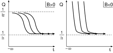
Figure 4: Classical solutions $Q(t)$ for $A>0$.

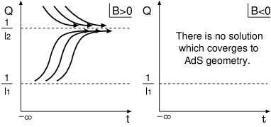
Figure 5: Classical solutions $Q(t)$ for $A<0$.

Figure 6: Result of the numerical calculation of classical solutions $Q(\tau)$ for the values $d=4$, $A=0.1$, $B=0.1$ and $l=1$ ($1/l_{1}=1$ and $1/l_{2}=6.24$).

Now we give a holographic RG interpretation to the above results. We first consider the AdS⁽¹⁾ solution. Looking at the equation (2.27), the equation (5.21) is nothing but the equation of motion of a scalar field in the AdS background of radius $l$, with mass squared given by

$$m_{1}^{2} =-{2\over A}\left(2\Lambda l^{2}+{3B\over l^{2}}\right)$$

$$={2\over A}\left(d(d-1)-{6B\over l^{2}}\right).$$ (5.25)

Thus for $A>0$, the higher-derivative mode $Q$ is interpreted as a very massive scalar mode, and thus it is coupled to a highly irrelevant operator around the fixed point, since its scaling dimension is given by [6, 7]

$$\Delta={d\over 2}+\sqrt{{d^{4}\over 4}+l^{2}m_{1}^{2}}\gg d.$$ (5.26)

This can also be understood from Fig. 4 which depicts a rapid convergence of the RG flow to the fixed point $Q(t)=1/l$. On the other hand, for $A<0$, the mass squared of the higher-derivative mode is far below the lower bound for a scalar mode in the AdS⁽¹⁾ geometry, $-d^{2}/4l^{2}$ [7], and the scaling dimension becomes complex. Thus, in this case, the higher-derivative mode makes the AdS⁽¹⁾ geometry unstable, and a holographic RG interpretation cannot be given to such a solution.

We note here that, to obtain the original CFT dual to the AdS⁽¹⁾ as the continuum limit is taken, $t\to-\infty$, we must fix the higher-derivative mode at the stationary point, $Q=1/l_{1}$. Roughly speaking, this is realized by tuning the boundary value of the conjugate momentum of the higher-derivative mode to be zero. In the next subsection, we adopt this boundary condition to derive the flow equation for the $R^{2}$ gravity theory.

We next consider the AdS⁽²⁾. For $A>0$ and $B>0$ in Fig. 4, it can be seen that classical trajectories begin from AdS⁽²⁾ to AdS⁽¹⁾. In the context of the holographic RG, this means that the AdS⁽²⁾ solution $Q(t)=1/l_{2}$ corresponds to a multicritical point in the phase diagram of the boundary field theory. From (5.19) and (5.22), the mass squared of the mode $Q$ around the AdS⁽²⁾ can be calculated as

$$m_{2}^{2}=-{2\over A}\left(d(d-1)-{6B\over l^{2}}\right),$$ (5.27)

and if this mass squared is above the unitarity bound,

$$l_{2}^{2}m_{2}^{2}=-{6B\over A}{d(d-1)l^{2}-6B\over d(d-1)l^{2}-3B}>-{d^{2}\over 4},$$ (5.28)

the scaling dimension of the corresponding operator is given by

$$\Delta={d\over 2}+\sqrt{{d^{2}\over 4}+l_{2}^{2}m_{2}^{2}}\,\cong\,{d\over 2}+\sqrt{{d^{2}\over 4}-{6B\over A}}.$$ (5.29)

For example, if we consider the case in which $d=4$, $a=b=0$ and $c>0$, we have $A=32c>0$ and $B=8c/3>0$, and thus the scaling dimension of $Q$ around the AdS⁽²⁾ is found to be $\Delta\cong 2+\sqrt{7/2}$. It would be interesting to investigate which conformal field theory describes this fixed point.

We conclude this subsection with a comment on the $c$-theorem. Since the trace of the extrinsic curvature, $\widehat{K}{}$, is given by $\widehat{K}{}\sim Q$ in the block spin gauge, we see from Eq. (2.72) (or Eq. (3.80)) that the $c$-function [16] is given by $c(Q)=Q^{1-d}$. Fig. 3 shows that it increases when $A>0$, but this does not contradict the assertion of the $c$-theorem, because in this case, the kinetic term of $Q(t)$ in the bulk action has a negative sign. This suggests that the obtained multicritical point defines a nonunitary theory like a Lee-Yang edge singularity.

5.2 Hamilton-Jacobi equation for a higher-derivative Lagrangian

In the previous subsection, we pointed out that the boundary value of the higher-derivative mode must be at a stationary point in order to implement the continuum limit of the boundary field theory. To clarify this point further, in this subsection, we give a detailed discussion on the boundary conditions for higher-derivative modes that incorporate the idea of the holographic RG. We here discuss a point particle system, and will extend our analysis to systems of higher-derivative gravity in the next subsection.

A dynamical system with the action

$$\mbox{\boldmath$S$}\bigl{[}q(\tau)\bigr{]}=\int_{t^{\prime}}^{t}d\tau\,L\left(q,\dot{q},\ddot{q}\right)$$ (5.30)

is described by the equation of motion which is a fourth-order differential equation in time $\tau$;

$${d^{2}\over d\tau^{2}}\left({\partial L\over\partial\ddot{q}}\right)-{d\over d\tau}\left({\partial L\over\partial\dot{q}}\right)+{\partial L\over\partial{q}}=0.$$ (5.31)

This implies that we need four boundary conditions to determine the classical solution uniquely. Possible boundary conditions can be found most easily by rewriting the system into the Hamiltonian formalism with an extra set of canonical variables $(Q,P)$ which represents $\dot{q}$ and its canonical momentum.

The Lagrangian in (5.30) is classically equivalent to

$$L^{\prime}(q,Q,\dot{Q};p)=L\left(q,Q,\dot{Q}\right)+p\left(\dot{q}-Q\right),$$ (5.32)

where $p$ is a Lagrange multiplier. We then carry out a Legendre transformation from $(Q,\dot{Q})$ to $(Q,P)$ through

$$P={\partial L^{\prime}\over\partial\dot{Q}}\bigl{(}q,Q,\dot{Q};p\bigr{)}\,.$$ (5.33)

Assuming that this equation can be solved with respect to $\dot{Q}$ $\left(\equiv\dot{Q}\!\left(q,Q;P\right)\right)$, we introduce the Hamiltonian

$$H(q,Q;\,p,P)\equiv p\,Q+P\dot{Q}\!\left(q,Q;\,P\right)-\,L\left(q,Q,\dot{Q}\!\left(q,Q;\,P\right)\right),$$ (5.34)

and rewrite the action (5.30) in the first-order form;

$$\mbox{\boldmath$S$}[q,Q;\,p,P]=\int^{t}_{t^{\prime}}d\tau\left[p\,\dot{q}+P\dot{Q}-H(q,Q;\,p,P)\right],$$ (5.35)

where $\dot{Q}$ is now the time-derivative of the independent variable $Q$. The variation of the action (5.35) reads

$$\delta\mbox{\boldmath$S$}= \int^{t}_{t^{\prime}}d\tau\left[\,\delta p\left(\dot{q}-{\partial H\over\partial p}\right)+\delta P\left(\dot{Q}-{\partial H\over\partial P}\right)\right.$$

$$\hskip 36.98857pt\left.-\,\delta q\left(\dot{p}+{\partial H\over\partial q}\right)-\delta Q\left(\dot{P}+{\partial H\over\partial Q}\right)\right]$$

$$~{}~{}+\left(p\,\delta q+P\,\delta Q\right)\Big{|}^{t}_{t^{\prime}}\,,$$ (5.36)

and thus the equation of motion consists of the usual Hamilton equations,

$$\dot{q}={\partial H\over\partial p},\quad\dot{Q}={\partial H\over\partial P},\quad\dot{p}=-{\partial H\over\partial q},\quad\dot{P}=-{\partial H\over\partial Q}\,,$$ (5.37)

plus the following constraints which must hold at the boundary, $\tau=t$ and $\tau=t^{\prime}$:

$$p\,\delta q+P\,\delta Q=0\quad(\tau=t,t^{\prime})\,.$$ (5.38)

The latter requirement, (5.38), can be satisfied by imposing either Dirichlet boundary conditions,

$${\rm\underline{Dirichlet}:}\qquad\delta q=0\,,\quad\delta Q=0\quad(\tau=t,t^{\prime})\,,$$ (5.39)

or Neumann boundary conditions,

$${\rm\underline{Neumann}:}\qquad p=0\,,\quad P=0\quad(\tau=t,t^{\prime})\,,$$ (5.40)

for each variable $q$ and $Q$. If, for example, we take the classical solution $(\overline{q},\overline{Q},\overline{p},\overline{P})$ that satisfies the Dirichlet boundary conditions for all $(q,Q)$ with specified boundary values as

$$\overline{q}(\tau\!=\!t)=q,~{}\overline{Q}(\tau\!=\!t)=Q,\quad~{}{\rm and}\quad\overline{q}(\tau\!=\!t^{\prime})=q^{\prime},~{}\overline{Q}(\tau\!=\!t^{\prime})=Q^{\prime}\,,$$ (5.41)

then after plugging the solution into the action, we obtain the classical action that is a function of these boundary values,

$$S\bigl{(}t,q,Q;\,t^{\prime},q^{\prime},Q^{\prime}\bigr{)}=\mbox{\boldmath$S$}\left[\overline{q}(\tau),\overline{Q}(\tau);\,\overline{p}(\tau),\overline{P}(\tau)\right].$$ (5.42)

However, this classical action is not relevant to us in the context of the AdS/CFT correspondence, since we must further set the boundary value $Q$ of the higher-derivative mode to a stationary point in order to implement the continuum limit of the boundary field theory. This requirement is equivalent to the condition that the higher-derivative mode has vanishing momentum. We are thus led to use mixed boundary conditions [39]:

$$\delta q=0\quad{\rm and}\quad P=0\qquad(\tau=t,\,t^{\prime})\,,$$ (5.43)

that is, we impose the Dirichlet boundary conditions for $q$ and Neumann boundary conditions for $Q$. In this case, the classical action (to be called the reduced classical action) becomes a function only of the boundary values $q$ and $q^{\prime}$:

$$S=S(t,q;\,t^{\prime},q^{\prime})\,.$$ (5.44)

If we further demand the regular behavior in taking $t\rightarrow+\infty$, the classical action depends only on the initial value. The same argument can be applied to dynamical systems of $(d+1)$-dimensional fields with higher-derivative interactions of arbitrary order [39]. Furthermore, the discussion in the previous subsection shows that higher-derivative modes should take stationary values in order to get a finite result in approaching the boundary. This supports our expectation that for any bulk system of gravity with higher-derivative interactions, if we require the regularity inside the bulk and the finiteness near the boundary, the Euclidean time development is completely determined only by the boundary values of the original fields. That is, the holographic nature still exists for higher-derivative systems.

Now we derive an equation that determines the reduced classical action (5.44). This can be derived in two ways, and we first explain a more complicated, but straightforward, way since this gives us a deeper understanding of the mathematical structure. To this end, we first change the polarization of the system by performing the canonical transformation

$$\widehat{\mbox{\boldmath$S$}}\equiv\mbox{\boldmath$S$}-\int^{t}_{t^{\prime}}d(PQ)\,.$$ (5.45)

Although the Hamilton equation does not change under this transformation, the boundary conditions at $\tau=t$ and $\tau=t^{\prime}$ become

$$p\,\delta q-Q\delta P=0\quad(\tau=t,t^{\prime})\,.$$ (5.46)

These boundary conditions can be satisfied by imposing the Dirichlet boundary conditions for both $\overline{q}$ and $\overline{P}$:

$$\overline{q}(\tau\!=\!t)=q,~{}\overline{P}(\tau\!=\!t)=P\,,\quad{\rm and}\quad\overline{q}(\tau\!=\!t^{\prime})=q^{\prime},~{}\overline{P}(\tau\!=\!t^{\prime})=P^{\prime}\,.$$ (5.47)

Substituting this solution into $\widehat{\mbox{\boldmath$S$}}$, we obtain a new classical action that is a function of these boundary values,

$$\widehat{S}\left(t,q,P;\,t^{\prime},q^{\prime},P^{\prime}\right)=\widehat{\mbox{\boldmath$S$}}\left[\overline{q}(\tau),\overline{Q}(\tau);\,\overline{p}(\tau),\overline{P}(\tau)\right].$$ (5.48)

By taking the variation of $\widehat{\mbox{\boldmath$S$}}$ and using the equation of motion, we can easily show that the new classical action $\widehat{S}$ obeys the Hamilton-Jacobi equation:

$${\partial\widehat{S}\over\partial t} = -H\left(q,-{\partial\widehat{S}\over\partial P};\,+{\partial\widehat{S}\over\partial q},P\right),$$

$${\partial\widehat{S}\over\partial t^{\prime}} = +H\left(q^{\prime},+{\partial\widehat{S}\over\partial P^{\prime}};\,-{\partial\widehat{S}\over\partial q^{\prime}},P^{\prime}\right).$$ (5.49)

The reduced classical action $S(t,q;t^{\prime},q^{\prime})$ is then obtained by setting $P\!=\!0$ in $\widehat{S}$:

$$S\left(t,q;t^{\prime},q^{\prime}\right)=\widehat{S}\left(t,q,P\!=\!0;\,t^{\prime},q^{\prime},P^{\prime}\!=\!0\right).$$ (5.50)

Note that the generating function $PQ$ vanishes at the boundary when we set $P\!=\!0$. In Appendix E, we briefly describe how the Hamilton-Jacobi equation (5.49) is solved for a system of a point particle.

In solving the full Hamilton-Jacobi equation, we must impose the regularity for $\widehat{S}(t,q,P)$ in the limit $c\!=\!0$ when $P\!=\!0$. This is because the higher-derivative term is regarded as a perturbation and the reduced classical action must have a finite limit for $c\!\rightarrow\!0$. One can see that the Hamilton-Jacobi equation reduces to an equation involving the reduced action. We call it a Hamilton-Jacobi-like equation. However, once the regularity condition is imposed, we have an alternative way to derive the Hamilton-Jacobi-like equation with greater ease. In fact, for any Lagrangian of the form

$$L(q^{i},\dot{q}^{i},\ddot{q}^{i})=L_{0}(q^{i},\dot{q}^{i})+c\,L_{1}(q^{i},\dot{q}^{i},\ddot{q}^{i})\,,$$ (5.51)

one can prove the following theorem, assuming that the classical solution can be expanded around $c\!=\!0$:

Theorem [39]
Let $H_{0}(q,p)$ be the Hamiltonian corresponding to $L_{0}(q,\dot{q})$. Then the reduced classical action $S(t,q;\,t^{\prime},q^{\prime})\!=\!S_{0}(t,q;\,t^{\prime},q^{\prime})+c\,S_{1}(t,q;\,t^{\prime},q^{\prime})+{\cal O}(c^{2})$ satisfies the following equation up to ${\cal O}(c^{2})$:

$$-{\partial S\over\partial t}=\widetilde{H}(q,p),\quad p_{i}={\partial S\over\partial q^{i}},\quad{\rm and}\quad+{\partial S\over\partial t^{\prime}}=\widetilde{H}(q^{\prime},p^{\prime}),\quad p^{\prime}_{i}=-{\partial S\over\partial q^{\prime\,i}},$$ (5.52)

where

$$\widetilde{H}(q,p) \equiv H_{0}(q,p)-c\,L_{1}(q,f_{1}(q,p),f_{2}(q,p)),$$

$$f_{1}^{i}(q,p) \equiv \left\{H_{0},q^{i}\right\}={\partial H_{0}\over\partial p_{i}},$$

$$f_{2}^{i}(q,p) \equiv \left\{H_{0},\left\{H_{0},q^{i}\right\}\right\}={\partial^{2}H_{0}\over\partial p_{i}\partial q^{j}}{\partial H_{0}\over\partial p_{j}}-{\partial^{2}H_{0}\over\partial p_{i}\partial p_{j}}{\partial H_{0}\over\partial q^{j}}.$$ (5.53)

$$\left(\left\{F(q,p),G(q,p)\right\}\equiv\frac{\partial F}{\partial p_{i}}\frac{\partial G}{\partial q^{i}}-\frac{\partial G}{\partial p_{i}}\frac{\partial F}{\partial q^{i}}\right)$$

We call $\widetilde{H}$ a pseudo-Hamiltonian.

A proof of this theorem is given in Appendix F. One can see easily that this correctly reproduces (E.11) and (E.12) for the Lagrangian given in (E.1)–(E.3).

5.3 Application to higher-derivative gravity

Here we apply the formalism developed in the previous subsection to a system of higher-derivative gravity with the action (5.13). We first derive the Hamilton-Jacobi-like equation of the system. We also show that the coefficients $x_{1},\cdots,x_{5}$ must obey some relations so that we can impose the mixed boundary condition consistently.

The action (5.13) is expressed in terms of the ADM parametrization as

$$\mbox{\boldmath$S$}=\int_{\tau_{0}}^{\infty}d\tau\int d^{d}x\sqrt{\widehat{g}{}}\,\left[\mbox{\boldmath${\cal L}$}_{0}\bigl{(}\widehat{g}{},\widehat{K}{};\,N,\widehat{\lambda}{}\bigr{)}+\mbox{\boldmath${\cal L}$}_{1}\bigl{(}\widehat{g}{},\widehat{K}{},\dot{\widehat{K}{}};\,\widehat{N},\widehat{\lambda}{}\bigr{)}\right],$$ (5.54)

where

$$\frac{1}{\widehat{N}}\,\mbox{\boldmath${\cal L}$}_{0} = 2\Lambda-\widehat{R}{}+\widehat{K}{}_{ij}^{2}-\widehat{K}{}^{2},$$ (5.55)

$$\frac{1}{\widehat{N}}\,\mbox{\boldmath${\cal L}$}_{1} = -a\widehat{R}{}^{2}-b\widehat{R}{}_{ij}^{2}-c\widehat{R}{}_{ijkl}^{2}+\Big{[}(-6a+2x_{1})\widehat{K}{}_{ij}^{2}+(2a-x_{1})\widehat{K}{}^{2}\Big{]}\widehat{R}{}$$ (5.56)

$$+\Big{[}-2(2b+4c-x_{2})(\widehat{K}{}^{2})_{ij}+(2b+2x_{1}-x_{2})\widehat{K}{}\widehat{K}{}_{ij}\Big{]}\widehat{R}{}^{ij}$$

$$+\,2(6c+x_{2})\widehat{K}{}_{ik}\widehat{K}{}_{jl}\widehat{R}{}^{ijkl}$$

$$-\,2(2b+c-3x_{5})\widehat{K}{}_{ij}^{4}+(4b+4x_{4}-x_{5})\widehat{K}{}\widehat{K}{}_{ij}^{3}$$

$$-\,(9a+b+2c-2x_{4})\left(\widehat{K}{}_{ij}^{2}\right)^{2}+(6a-b+6x_{3}-x_{4})\widehat{K}{}^{2}\widehat{K}{}_{ij}^{2}$$

$$-\,(a+x_{3})\widehat{K}{}^{4}$$

$$-\,(4b+2x_{1}-x_{2})\widehat{K}{}_{ij}\widehat{\nabla}{}^{i}\widehat{\nabla}{}^{j}\widehat{K}{}+2(b-4c+x_{2})\widehat{K}{}_{ij}\widehat{\nabla}{}^{j}\widehat{\nabla}{}_{k}\widehat{K}{}^{ki}$$

$$+\,(8c+x_{2})\widehat{K}{}_{ij}\widehat{\nabla}{}^{2}\widehat{K}{}^{ij}+2(b+x_{1})\widehat{K}{}\widehat{\nabla}{}^{2}\widehat{K}{}$$

$$-\Big{[}(4a+b)\widehat{g}{}^{ij}\widehat{g}{}^{kl}+(b+4c)\widehat{g}{}^{ik}\widehat{g}{}^{jl}\Big{]}\widehat{L}{}_{ij}\widehat{L}{}_{kl}$$

$$+\bigg{[}\Big{\{}(4a-x_{1})\widehat{R}{}+(12a+2b-x_{4})\widehat{K}{}_{kl}^{2}-(4a+3x_{3})\widehat{K}{}^{2}\Big{\}}\widehat{g}{}^{ij}$$

$$~{}~{}~{}+(2b-x_{2})\widehat{R}{}^{ij}+(4b+8c-3x_{5})(\widehat{K}{}^{2})^{ij}-2(b+x_{4})\widehat{K}{}\widehat{K}{}^{ij}\bigg{]}\widehat{L}{}_{ij},$$

with

$$\widehat{K}{}_{ij}=\frac{1}{2\widehat{N}}\left(\dot{\widehat{g}{}}_{ij}-\widehat{\nabla}{}_{i}\widehat{\lambda}{}_{j}-\widehat{\nabla}{}_{j}\widehat{\lambda}{}_{i}\right),$$ (5.57)

and

$$\widehat{L}{}_{ij}=\frac{1}{\widehat{N}}\left(\dot{\widehat{K}{}}_{ij}-\widehat{\lambda}{}^{k}\,\widehat{\nabla}{}_{k}\widehat{K}{}_{ij}-\widehat{\nabla}{}_{i}\widehat{\lambda}{}^{k}\,\widehat{K}{}_{kj}-\widehat{\nabla}{}_{j}\widehat{\lambda}{}^{k}\,\widehat{K}{}_{ik}+\widehat{\nabla}{}_{i}\widehat{\nabla}{}_{j}\widehat{N}\right)\,.$$ (5.58)

For details of the ADM decomposition, see Appendix C.

We now derive the Hamilton-Jacobi-like equation of $R^{2}$ gravity by using the Theorem, (5.52) and (5.53). We first rewrite the Lagrangian density of zero-th order, $\mbox{\boldmath${\cal L}$}_{0}$, into the first-order form

$$\mbox{\boldmath${\cal L}$}_{0}\rightarrow\widehat{\pi}{}^{ij}\dot{\widehat{g}{}}_{ij}-\mbox{\boldmath${\cal H}$}_{0}\,,$$ (5.59)

where the zero-th order Hamiltonian density $\mbox{\boldmath${\cal H}$}_{0}$ is given by

$$\mbox{\boldmath${\cal H}$}_{0}\bigl{(}\widehat{g}{},\widehat{\pi}{};\,\widehat{N},\widehat{\lambda}{}\bigr{)}=\widehat{N}\,\left(\widehat{\pi}{}_{ij}^{2}-{1\over d-1}\widehat{\pi}{}^{2}-2\Lambda+\widehat{R}{}\right)-2\widehat{\lambda}{}_{i}\,\widehat{\nabla}{}_{j}\widehat{\pi}{}^{ij}\,.$$ (5.60)

Then by using the Theorem, the pseudo-Hamiltonian density is given by

$$\widetilde{\mbox{\boldmath${\cal H}$}}\bigl{(}\widehat{g}{},\widehat{\pi}{};\,\widehat{N},\widehat{\lambda}{}\bigr{)}=\mbox{\boldmath${\cal H}$}_{0}\bigl{(}\widehat{g}{},\widehat{\pi}{};\,\widehat{N},\widehat{\lambda}{}\bigr{)}-\mbox{\boldmath${\cal L}$}_{1}\bigl{(}\widehat{g}{},\widehat{K}{}^{0}(g,\pi),\widehat{K}{}^{1}(\widehat{g}{},\widehat{\pi}{});\,\widehat{N},\widehat{\lambda}{}\bigr{)}\,.$$ (5.61)

Here $\widehat{K}{}^{0}_{ij}(\widehat{g}{},\widehat{\pi}{})$ is obtained by replacing $\dot{\widehat{g}{}}_{ij}(x)$ in (5.57) with $\left\{\int d^{d}y\sqrt{\widehat{g}{}}\,\mbox{\boldmath${\cal H}$}_{0}(y),\,\widehat{g}{}_{ij}(x)\right\}$, and it is calculated to be

$$\widehat{K}{}^{0}_{ij}=\widehat{\pi}{}_{ij}-{1\over d-1}\widehat{\pi}{}\,\widehat{g}{}_{ij}\,.$$ (5.62)

On the other hand, $\widehat{K}{}^{1}_{ij}\equiv\left\{\int d^{d}y\sqrt{\widehat{g}{}}\,\mbox{\boldmath${\cal H}$}_{0}(y),\,\widehat{K}{}^{0}_{ij}\right\}$ is found to be equivalent to replacing $\widehat{L}{}_{ij}$ in $\mbox{\boldmath${\cal L}$}_{1}$ by

$$\widehat{L}{}^{0}_{ij}= \,-{1\over 2(d-1)^{2}}\Bigl{[}2(d-1)\Lambda+(d-1)\widehat{R}{}+(d-1)\widehat{\pi}{}_{kl}^{2}-3\widehat{\pi}{}^{2}\Bigr{]}\widehat{g}{}_{ij}$$

$$~{}+\widehat{R}{}_{ij}+2(\widehat{\pi}{}^{2})_{ij}-{3\over d-1}\widehat{\pi}{}\widehat{\pi}{}_{ij}\,.$$ (5.63)

Using Eqs. (5.59)–(5.63), we obtain the following Hamilton-Jacobi-like equation for the reduced classical action [39]:

$$0 \!=\! \int d^{d}x\sqrt{g}\,\widetilde{\mbox{\boldmath${\cal H}$}}\left(g(x),\pi(x);N(x),\lambda^{i}(x)\right)$$ (5.64)

$$\!=\! \int d^{d}x\sqrt{g}\,\left[N(x)\,\widetilde{{\cal H}}(g(x),\pi(x))+\lambda^{i}(x)\,\widetilde{{\cal P}}_{i}(g(x),\pi(x))\right]\,,$$

$$\pi^{ij}(x)=\frac{-1}{\sqrt{g}}\frac{\delta S}{\delta g_{ij}(x)}\,,$$ (5.65)

where $g_{ij}$ and $\pi^{ij}$ are the boundary values of $\widehat{g}{}_{ij}$ and $\widehat{\pi}{}^{ij}$, respectively, and

$$\widetilde{{\cal H}}(g,\pi) \equiv \pi_{ij}^{2}-{1\over d-1}\pi^{2}-2\Lambda+R$$ (5.66)

$$+\,\alpha_{1}\,\pi_{ij}^{4}+\alpha_{2}\,\pi\pi_{ij}^{3}+\alpha_{3}\left(\pi_{ij}^{2}\right)^{2}+\alpha_{4}\,\pi^{2}\pi_{ij}^{2}+\alpha_{5}\,\pi^{4}$$

$$+\,\beta_{1}\,\Lambda\pi_{ij}^{2}+\beta_{2}\,\Lambda\pi^{2}+\beta_{3}\,R\,\pi_{ij}^{2}+\beta_{4}\,R\,\pi^{2}$$

$$+\,\beta_{5}\,R_{ij}(\pi^{2})^{ij}+\beta_{6}\,R_{ij}\,\pi\pi^{ij}+\beta_{7}\,R_{ijkl}\,\pi^{ik}\pi^{jl}$$

$$+\,\gamma_{1}\,\Lambda^{2}+\gamma_{2}\,\Lambda R+\gamma_{3}\,R^{2}+\gamma_{4}\,R_{ij}^{2}+\gamma_{5}\,R_{ijkl}^{2}\,,$$

$$\widetilde{{\cal P}}_{i}(g,\pi) \equiv -2\nabla^{j}\pi_{ij}\,,$$ (5.67)

with

$$\alpha_{1}= \,2c,\quad\alpha_{2}={2x_{5}\over(d-1)},$$

$$\alpha_{3}= \,{1\over 4(d-1)^{2}}\Big{[}4a+(d^{2}-3d+4)b+4(d-2)(2d-3)c$$

$$\qquad\qquad~{}~{}-2(d-1)(dx_{4}+3x_{5})\Big{]},$$

$$\alpha_{4}= \,{1\over 2(d-1)^{3}}\left[-4a-(d^{2}-3d+4)b-4(2d^{2}-5d+4)c\right.$$

$$\left.\qquad\qquad~{}~{}-3dx_{3}+(2d^{2}-7d+2)x_{4}-3(2d-1)x_{5}\right],$$

$$\alpha_{5}= \,{1\over 4(d-1)^{4}}\left[4a+(d^{2}-3d+4)b+4(2d^{2}-5d+4)c\right.$$

$$\left.\qquad\qquad~{}~{}+2(3d-4)x_{3}-2(d^{2}-6d+6)x_{4}+2(5d-6)x_{5}\right],$$ (5.68)

$$\beta_{1}= \,{1\over(d-1)^{2}}\Big{[}4da-d(d-3)b-4(d-2)c-(d-1)(dx_{4}+3x_{5})\Big{]},$$

$$\beta_{2}= \,{1\over(d-1)^{3}}\Big{[}-4da+d(d-3)b+4(d-2)c$$

$$\qquad\qquad~{}~{}-3dx_{3}+(d^{2}-2d-2)x_{4}+3(d-2)x_{5}\Big{]},$$

$$\beta_{3}= \,{1\over 2(d-1)^{2}}\Big{[}4a+(d^{2}-3d+4)b-4(3d-4)c$$

$$\qquad\qquad~{}~{}-(d-1)(dx_{1}+x_{2}-(d-2)x_{4}+3x_{5})\Big{]},$$

$$\beta_{4}= \,{1\over 2(d-1)^{3}}\Big{[}-4a-(d^{2}-3d+4)b+4(d-2)c$$

$$\qquad\qquad~{}~{}-(d-1)(d-4)x_{1}-3(d-1)x_{2}+3(d-2)x_{3}$$

$$\qquad\qquad~{}~{}-(d^{2}-8d+10)x_{4}+3(3d-4)x_{5}\Big{]},$$

$$\beta_{5}= \,16c+3x_{5},\qquad\beta_{6}={2(x_{1}+2x_{2}-x_{4}-3x_{5})\over d-1},\qquad\beta_{7}=-12c-2x_{2},$$ (5.69)

$$\gamma_{1} = {d\over(d-1)^{2}}\Big{[}4da+(d+1)b+4c\Big{]},$$

$$\gamma_{2} = {1\over(d-1)^{2}}\Big{[}4da-d(d-3)b-4(d-2)c-(d-1)(dx_{1}+x_{2})\Big{]},$$

$$\gamma_{3} = {1\over 4(d-1)^{2}}\Big{[}4a+(d^{2}-3d+4)b-4(3d-4)c+2(d-1)((d-2)x_{1}-x_{2})\Big{]},$$

$$\gamma_{4} = 4c+x_{2},\qquad\gamma_{5}=c.$$ (5.70)

Here $R_{ijkl}$ is the Riemann tensor made of the metric tensor of the $d$-dimensional boundary $\tau=\tau_{0}$. Since the (true) classical action $\widehat{S}{}[g(x),P(x)]$ is independent of the choice of $N$ and $\lambda^{i}$ (and thus, so is $S[g(x)]$), from Eqs. (5.64)–(5.67) we finally obtain the following equation that determines the reduced classical action:

$$\widetilde{{\cal H}}\bigl{(}g_{ij}(x),\pi^{ij}(x)\bigr{)}=0\,,\quad\widetilde{{\cal P}}_{i}\bigl{(}g_{ij}(x),\pi^{ij}(x)\bigr{)}=0\,,\quad\pi^{ij}(x)=\frac{-1}{\sqrt{g}}\frac{\delta S}{\delta g_{ij}(x)}\,.$$ (5.71)

We make a few comments on the possible form of the boundary action $\mbox{\boldmath$S$}_{b}$ and the cosmological constant $\Lambda$. As discussed above, in order that the boundary field theory has a continuum limit, the geometry must be asymptotically AdS:

$$ds^{2}\rightarrow d\tau^{2}+e^{-2\tau/l}\eta_{ij}(x)dx^{i}dx^{j}\quad{\rm for}~{}~{}\tau\rightarrow-\infty.$$ (5.72)

This should be consistent with our boundary condition $P^{ij}\!=\!0$. Explicitly investigating the equations of motion derived from the action (5.54), we can show that this compatibility gives rise to the relation

$$d^{2}\,x_{3}+d\,x_{4}+x_{5} = -{4\over 3}\Big{(}d(d+1)a+db+2c\Big{)}.$$ (5.73)

It can also be shown that the asymptotic behavior (5.72) determines the cosmological constant $\Lambda$ as

$$\Lambda=-{d(d-1)\over 2l^{2}}+{d(d-3)\over 2l^{4}}\Big{[}d(d+1)a+db+2c\Big{]}.$$ (5.74)

5.4 Solution to the flow equation and the Weyl anomaly

We first note that the basic equation, (5.71), can be rewritten as a flow equation of the form [39]

$$\{S,S\}+\{S,S,S,S\}={\cal L}_{d},$$ (5.75)

with

$$\left(\sqrt{g}\right)^{2}\,\{S,S\}\equiv \,\left[\left({\delta S\over\delta g_{ij}}\right)^{2}-{1\over d-1}\left(g_{ij}{\delta S\over\delta g_{ij}}\right)^{2}\right.$$

$$\left.~{}+\beta_{1}\,\Lambda\left({\delta S\over\delta g_{ij}}\right)^{2}+\beta_{2}\,\Lambda\left(g_{ij}{\delta S\over\delta g_{ij}}\right)^{2}+\beta_{3}\,R\left({\delta S\over\delta g_{ij}}\right)^{2}\right.$$

$$\left.~{}+\beta_{4}\,R\left(g_{ij}{\delta S\over\delta g_{ij}}\right)^{2}+\beta_{5}\,R_{ij}g_{kl}{\delta S\over\delta g_{ik}}{\delta S\over\delta g_{jl}}\right.$$

$$\left.~{}+\beta_{6}\,R_{ij}{\delta S\over\delta g_{ij}}\,g_{kl}{\delta S\over\delta g_{kl}}+\beta_{7}\,R_{ijkl}{\delta S\over\delta g_{ik}}\,{\delta S\over\delta g_{jl}}\right],$$ (5.76)

$$\left(\sqrt{g}\right)^{4}\{S,S,S,S\} \equiv \left[\alpha_{1}\left({\delta S\over\delta g_{ij}}\right)^{4}+\alpha_{2}\left(g_{kl}{\delta S\over\delta g_{kl}}\right)\left({\delta S\over\delta g_{ij}}\right)^{3}+\alpha_{3}\left(\left({\delta S\over\delta g_{ij}}\right)^{2}\right)^{2}\right.$$ (5.77)

$$\left.~{}+\alpha_{4}\left(g_{kl}{\delta S\over\delta g_{kl}}\right)^{2}\left({\delta S\over\delta g_{ij}}\right)^{2}+\alpha_{5}\left(g_{ij}{\delta S\over\delta g_{ij}}\right)^{4}\right],$$

$${\cal L}_{d} \equiv 2\Lambda-R-\gamma_{1}\Lambda^{2}-\gamma_{2}\Lambda R-\gamma_{3}R^{2}-\gamma_{4}R_{ij}^{2}-\gamma_{5}R_{ijkl}^{2}.$$ (5.78)

As in §3, we decompose the reduced classical action into the local part and the non-local part,

$$\frac{1}{2\kappa_{d+1}^{2}}S[g(x)]=\frac{1}{2\kappa_{d+1}^{2}}S_{\rm loc}[g(x)]-\Gamma[g(x)]\,.$$ (5.79)

Following the prescription given in §3, we first determine the weight $0$ and $2$ parts of the $S_{\rm loc}$,

$$\left[{{\cal L}_{\rm loc}}\right]_{0}=W\,,\qquad\left[{{\cal L}_{\rm loc}}\right]_{2}=-\Phi\,R,$$ (5.80)

$$W= \,-{2(d-1)\over l}+{1\over l^{3}}\Big{[}-4d(d+1)a-4db-8c+d(d^{2}x_{3}+dx_{4}+x_{5})\Big{]},$$

$$\Phi= \,{l\over d-2}-{2\over(d-1)(d-2)\,l}\Big{[}d(d+1)a+d\,b+2c\Big{]}$$

$$+{1\over l}\left[d\,x_{1}+x_{2}+{3(d^{2}x_{3}+d\,x_{4}+x_{5})\over 2(d-1)}\right],$$ (5.81)

where (5.74) has been used.

For $d=4$, the weight $4$ part of the flow equation is an equation that the generating functional $\Gamma$ obeys,

$$2\Big{[}\{{S_{\rm loc}},\,\Gamma\}\Big{]}_{4}+4\Big{[}\{{S_{\rm loc}},\,{S_{\rm loc}},\,{S_{\rm loc}},\,\Gamma\}\Big{]}_{4}$$

$$=\frac{1}{2\kappa_{5}^{2}}\left(\Big{[}\{{S_{\rm loc}},\,{S_{\rm loc}}\}\Big{]}_{4}+\Big{[}\{{S_{\rm loc}},\,{S_{\rm loc}},\,{S_{\rm loc}},\,{S_{\rm loc}}\}\Big{]}_{4}\right.$$

$$\hskip 99.58464pt+\,\gamma_{3}R^{2}+\gamma_{4}R_{ij}^{2}+\gamma_{5}R_{ijkl}^{2}\Bigr{)}.$$ (5.82)

From this, we can evaluate the trace of the stress tensor for the boundary field theory:

$$\langle T^{i}_{i}\rangle_{g}\equiv{2\over\sqrt{g}}\,g_{ij}{\delta\Gamma\over\delta g_{ij}}.$$ (5.83)

In fact, using the values in (5.81), we can show that the trace is given by [39]

$$\langle T^{i}_{i}\rangle_{g}={2l^{3}\over 2\kappa_{5}^{2}}\Biggl{[} \left({-1\over 24}+{5a\over 3l^{2}}+{b\over 3l^{2}}+{c\over 3l^{2}}\right)R^{2}+\left({1\over 8}-{5a\over l^{2}}-{b\over l^{2}}-{3c\over 2l^{2}}\right)R_{ij}^{2}$$

$$+{c\over 2l^{2}}R_{ijkl}^{2}\Biggr{]}\,.$$ (5.84)

This correctly reproduces the result obtained in Refs. [42] and [101], where the Weyl anomaly was calculated by perturbatively solving the equation of motion near the boundary and by looking at the logarithmically divergent term, as in Ref. [33].

For the case of ${\cal N}\!=\!2$ superconformal $USp(N)$ gauge theory in four dimensions, we choose $2\kappa_{5}^{2}$ such that

$${1\over 2\kappa_{5}^{2}}={{\rm Vol}(S^{5}/\mbox{\boldmath$Z$}_{2})\,({\rm radius~{}of~{}}S^{5}/\mbox{\boldmath$Z$}_{2})^{5}\over 2\kappa^{2}},$$ (5.85)

where $2\kappa^{2}=(2\pi)^{7}g_{s}^{2}$ is the ten-dimensional Newton constant [102], and the radius of $S^{5}/\mbox{\boldmath$Z$}_{2}$ could be set to $(8\pi g_{s}N)^{1/4}$ [43]. In this relation, we note the replacement $N\to 2N$ as compared to the $AdS_{5}\times S^{5}$ case. This is because here we must quantize the RR $5$-form flux over $S_{5}/\mbox{\boldmath$Z$}_{2}$ instead of over $S^{5}$ [41]. For the $AdS_{5}$ radius $l$, we may also set $l=(8\pi g_{s}N)^{1/4}$. Setting the values $a=b=0$ and $c/2l^{2}=1/32N+{\cal O}(1/N^{2})$, as determined in Ref. [42], we find that the Weyl anomaly (5.84) takes the form

$$\langle T^{i}_{i}\rangle_{g} = {N^{2}\over 2\pi^{2}}\left[\left({-1\over 24}+{1\over 48N}\right)R^{2}+\left({1\over 8}-{3\over 32N}\right)R_{ij}^{2}+{1\over 32N}R_{ijkl}^{2}\right]+{\cal O}(N^{0})\,.$$

This is different from the field theoretical result [36],

$$\langle T^{i}_{i}\rangle_{g} = {N^{2}\over 2\pi^{2}}\left[\left({-1\over 24}-{1\over 32N}\right)R^{2}+\left({1\over 8}+{1\over 16N}\right)R_{ij}^{2}+{1\over 32N}R_{ijkl}^{2}\right]+{\cal O}(N^{0})\,.$$

As was pointed out in Ref. [42], the discrepancy could be accounted for by possible corrections to the radius $l$ as well as to the five-dimensional Newton constant. In fact, if these corrections are

$$l=(8\pi g_{s}N)^{1/4}\left(1+\frac{\xi}{N}\right)\,,\quad\frac{1}{2\kappa_{5}^{2}}=\frac{{\rm Vol}(S^{5}/\mbox{\boldmath$Z$}_{2})\,(8\pi g_{s}N)^{5/4}}{2\kappa^{2}}\left(1+{\eta\over N}\right)\,,$$ (5.88)

then the field theoretical result is correctly reproduced for $3\xi+\eta=5/4$.

6 Conclusion

In this article, we have investigated various aspects of the AdS/CFT correspondence and the holographic renormalization group (RG).

In §2, we gave a review of the basic idea of the AdS/CFT correspondence and the holographic RG, and calculated the scaling dimensions of the scaling operators which are dual to bulk scalar fields in the AdS background. As a typical example of the AdS/CFT correspondence, we considered the duality between the ${\mathcal{N}}=4$ $SU(N)$ SYM₄ and Type IIB supergravity on AdS${}_{5}\times S^{5}$. As a consistency check for the duality, we showed the one-to-one correspondence between the short chiral primary multiplets of the CFT and the Kaluza-Klein spectra of supergravity. We also demonstrated the holographic description of RG flows that interpolate between a UV and an IR fixed points, by considering the example of an RG flow from the ${\mathcal{N}}=4$ $SU(N)$ SYM₄ to the ${\mathcal{N}}=1$ Leigh-Strassler fixed point. The “c-function” was defined from the view point of the holographic RG, and shown to obey an analog of Zamolodchikov’s c-theorem.

In §3, we explored the formulation of the holographic RG based on the Hamilton-Jacobi equation of bulk gravity given by de Boer, Verlinde and Verlinde. A systematic prescription for calculating the Weyl anomaly of the boundary CFT was proposed. We also derived the Callan-Symanzik equation for $n$-point functions in the boundary field theory. We calculated the scaling dimensions of scaling operators from the coefficients of the RG beta functions, and showed that they are in precise agreement with known results in the AdS/CFT correspondence. We explained how we take the continuum limit of the boundary field theory, and concluded that the holographic RG describes the so-called renormalized trajectory.

We discussed the holographic RG in the framework of the noncritical string theory in §4. In the holographic RG, we must introduce an IR cutoff to regularize the infinite volume of the bulk space-time, and the (Euclidean) time development of fields in the gravity theory is required to be regular interior of the bulk. We demonstrated that this basic requirement in the holographic RG can be understood naturally in the context of noncritical strings.

In §5, the holographic RG for $R^{2}$ gravity was investigated. In general, when we work in the Hamiltonian formalism, we must introduce new valuables which we call the “higher-derivative modes.” We introduced a parametrization of the metric in which the Euclidean time evolution of the system can be directly interpreted as an RG transformation of the boundary field theory. We examined classical solutions of the system under this parametrization. We found that the stability of an AdS solution depends on the coefficients of the curvature squared terms, and the fluctuation of the higher-derivative mode around a stable AdS solution is interpreted as a very massive scalar field in the background of the AdS space-time. In the AdS/CFT correspondence, this means that the fluctuation of the higher-derivative mode corresponds to a highly irrelevant operator of the boundary CFT. Thus, we must fix the boundary values of higher-derivative modes at stationary values in order to implement the continuum limit of the boundary field theory. We discussed that the condition is automatically satisfied by adopting the mixed boundary condition, that is, the Dirichlet boundary condition for the usual valuables and the Neumann boundary condition for the higher-derivative modes. We also discussed that when the coefficients of the curvature squared terms satisfy an appropriate condition, there appears another conformal fixed point in the parameter space of the boundary field theories.

Using the prescription with the mixed boundary conditions, we derived a Hamilton-Jacobi-like equation for $R^{2}$ gravity which describes RG flows of the dual field theory. As an application, we calculated the $1/N$ correction of the Weyl anomaly of ${\mathcal{N}}=2$ $USp(N)$ supersymmetric gauge theory in four dimensions. We found that the result is consistent with a field theoretical calculation.

We here make a comment on field redefinitions of bulk gravity in the context of the AdS/CFT correspondence [103]. The AdS/CFT correspondence should have the property that any physical quantities of the $d$-dimensional boundary field theory calculated from $(d+1)$-dimensional bulk gravity are invariant under field redefinitions of the fields in ten-dimensional supergravity. This is because ten-dimensional classical supergravity represents the on-shell structure of massless modes of superstrings, and the on-shell amplitudes (more precisely, the residues of one-particle poles of correlation functions for external momenta) should be invariant under redefinitions of fields [104] (see also Ref. [105] for discussions in the context of string theory).

As an example, let us show [103] that the holographic Weyl anomaly of the ${\mathcal{N}}=4$ $SU(N)$ SYM₄ does not change under the field redefinition of the ten-dimensional metric of the form

$$\mbox{\boldmath$G$}_{MN}\to\mbox{\boldmath$G$}_{MN}^{\prime}\equiv\mbox{\boldmath$G$}_{MN}+\alpha\mbox{\boldmath$R$}\mbox{\boldmath$G$}_{MN}+\beta\mbox{\boldmath$R$}_{MN}.$$ (6.1)

The bosonic part of the ten-dimensional Type IIB supergravity action is given by

$$\mbox{\boldmath$S$}_{10}=\frac{1}{2\kappa_{10}^{2}}\int d^{10}X\sqrt{-\mbox{\boldmath$G$}}\left[e^{-2\phi}\left(\mbox{\boldmath$R$}+4\left|d\phi\right|^{2}\right)-{1\over 4}\left|F_{5}\right|^{2}\right].$$ (6.2)

In the context of the AdS₅/CFT₄ correspondence, we are interested in the AdS₅$\times$$S^{5}$ solution that is realized as the near horizon limit of the black 3-brane solution:

$$ds^{2}=\frac{l^{2}}{r^{2}}\,dr^{2}+\frac{r^{2}}{l^{2}}\,\eta_{ij}\,dx^{i}dx^{j}+l^{2}\,d\Omega_{5}^{2},$$

$$(F_{5})_{r0123}=-{4\over g_{s}}\,{r^{3}\over l^{4}},\quad(F_{5})_{y^{1}\cdots y^{5}}={4\over g_{s}}\,l^{4},$$

$$e^{\phi}=g_{s}.$$ (6.3)

Here, $d\Omega_{5}^{2}$ is the metric of the unit five-sphere and $i,j\in\{0,1,2,3\}$. In this case, the AdS₅ and $S^{5}$ have the same radius, $l$, whose value is determined by the D3-brane charge as

$$l=(4\pi g_{s}N)^{1/4},$$ (6.4)

where $N$ is the number of the coincident D3-branes, and we have set the string length $l_{s}$ to $1$. The action of the effective five-dimensional gravity is given by compactifying the ten-dimensional action (6.2) on $S^{5}$:

$$\mbox{\boldmath$S$}_{5}={\pi^{3}l^{5}\over 2\kappa_{10}^{2}g_{s}^{2}}\int d^{5}x\sqrt{-\widehat{g}{}}\left({12\over l^{2}}+\widehat{R}{}\right).$$ (6.5)

The holographic Weyl anomaly calculated from this action is given in (3.64), which reproduces the Weyl anomaly of the ${\mathcal{N}}=4$ $SU(N)$ SYM₄ as mentioned in §3.3.

On the other hand, if we make the field redefinition (6.1), the obtained new ten-dimensional gravity action is

$$\widetilde{\mbox{\boldmath$S$}}_{10}[ \mbox{\boldmath$G$}_{MN}]\equiv\mbox{\boldmath$S$}_{10}[\mbox{\boldmath$G$}_{MN}+\alpha\mbox{\boldmath$R$}\mbox{\boldmath$G$}_{MN}+\beta\mbox{\boldmath$R$}_{MN}]$$

$$=\frac{1}{2\kappa_{10}^{2}}\int d^{10}X\sqrt{-\mbox{\boldmath$G$}}\Biggl{\{}e^{-2\phi}\biggl{[}\mbox{\boldmath$R$}+4\left|d\phi\right|^{2}+a\mbox{\boldmath$R$}^{2}+b\mbox{\boldmath$R$}_{MN}^{2}$$

$$\qquad\qquad\qquad\qquad\qquad\qquad\quad+a\mbox{\boldmath$R$}\left|d\phi\right|^{2}+b\,\mbox{\boldmath$R$}^{MN}\partial_{M}\phi\,\partial_{N}\phi\biggr{]}$$

$$\qquad\qquad-{1\over 4}\left|F_{5}\right|^{2}+{b\over 8}\,\mbox{\boldmath$R$}\left|F_{5}\right|^{2}-{b\over 4}\,{1\over 4!}\,\mbox{\boldmath$R$}_{MN}(F_{5})^{MPQRS}(F_{5})^{N}_{\ PQRS}\Biggr{\}}.$$ (6.6)

Here $a$ and $b$ are defined as

$$a=4\alpha+{1\over 2}\beta,\quad b=-\beta.$$ (6.7)

The AdS${}_{5}\times S^{5}$ solution for the action (6.6) is given by

$$ds^{2}=\left(1-{8b\over{l^{\prime}}^{2}}\right){{l^{\prime}}^{2}\over r^{2}}\,dr^{2}+{r^{2}\over{l^{\prime}}^{2}}\,\eta_{ij}\,dx^{i}dx^{j}+{l^{\prime}}^{2}d\Omega_{5}^{2},$$

$$(F_{5})_{r0123}={4\over g_{s}}\left(1+{8b\over{l^{\prime}}^{2}}\right){r^{3}\over{l^{\prime}}^{4}},\quad(F_{5})_{y^{1}\cdots y^{5}}={4\over g_{s}}\left(1-{8b\over{l^{\prime}}^{2}}\right){l^{\prime}}^{4},$$

$$e^{\phi}=g_{s},$$ (6.8)

where the new radius of the $S^{5}$ is related to $l$ by

$$l^{\prime}=\left(1+\frac{2b}{l^{2}}\right)l.$$ (6.9)

Note that after the field redefinition, the radius of $S^{5}$, $l^{\prime}$, differs from that of AdS₅, $L$, which is expressed as

$$L\equiv\left(1-{4b\over{l^{\prime}}^{2}}\right)l^{\prime}=\left(1-{2b\over l^{2}}\right)l.$$ (6.10)

From the solution (6.8), we compactify ten-dimensional spacetime on $S^{5}$ of radius $l^{\prime}$. Then, the (dimensionally reduced) five-dimensional action is obtained as

$$\widetilde{\mbox{\boldmath$S$}}_{5}=\frac{\pi^{3}{l^{\prime}}^{5}}{2\kappa_{10}^{2}g_{s}^{2}} \left(1+{40a+4b\over{l^{\prime}}^{2}}\right)\times$$

$$\int d^{5}x\sqrt{-\widehat{g}{}}\left[\left({12\over{l^{\prime}}^{2}}-{80a-80b\over{l^{\prime}}^{4}}\right)+\widehat{R}{}+a\widehat{R}{}^{2}+b\widehat{R}{}_{\mu\nu}^{2}\right].$$ (6.11)

This action has an AdS₅ solution with radius $\left(1-4b/{l^{\prime}}^{2}\right)l^{\prime}$, which is consistent with the AdS${}_{5}\times S^{5}$ solution (6.8). The corresponding Weyl anomaly is calculated by using the formula (5.84) as

$$\langle T_{i}^{i}\rangle ={2L^{3}\over 2\kappa_{5}^{2}}\left(1-{40a+8b\over{l^{\prime}}^{2}}\right)\left(-{1\over 24}R^{2}+{1\over 8}R_{ij}^{2}\right)$$

$$=\frac{2\pi^{3}{l^{\prime}}^{8}}{2\kappa_{10}^{2}g_{s}^{2}}\left(1-{16b\over{l^{\prime}}^{2}}\right)\left(-{1\over 24}R^{2}+{1\over 8}R_{ij}^{2}\right)$$

$$=\frac{2\pi^{3}l^{8}}{2\kappa_{10}^{2}g_{s}^{2}}\left(-{1\over 24}R^{2}+{1\over 8}R_{ij}^{2}\right)$$

$$={N^{2}\over 4\pi^{2}}\left(-{1\over 24}R^{2}+{1\over 8}R_{ij}^{2}\right).$$ (6.12)

This is identical to the result (3.64).

We conclude this article by making a few comments on future directions in the AdS/CFT correspondence and the holographic RG.

Once we start with AdS_d+1 gravity with $d\geq 4$, the dual $d$-dimensional conformal field theory is in general at a non-trivial fixed point, because operators of dual CFT coupled to bulk modes have non-trivial anomalous dimensions. It is thus natural to conjecture that any CFT in higher dimensions which has an AdS dual is a non-abelian gauge theory. In fact, all the known examples of the AdS/CFT correspondence involve non-abelian gauge theories. Furthermore, a non-trivial fixed point for $d\geq 4$ seems unlikely besides non-abelian gauge theories because of triviality. It would be nice to study the conjecture in more detail. In particular, it is interesting to investigate if there is a chance to gain information on the gauge symmetry of the boundary theory only from bulk supergravity.

The equation (3.30) seems to imply some hidden symmetry in bulk. In fact, the form of (3.30) is reminiscent of a scalar potential of supergravity with $W(\phi)$ a “superpotential.” Moreover, as pointed out in Ref. [16], holographic RG flows can be described by first-order differential equations via the superpotential. These facts might suggest that bulk gravity has a hidden supersymmetry or some novel symmetry.

To show the gauge/string duality from the loop equations of the Yang-Mills theory [108, 109] is an old but fascinating idea [110]-[116]. A strong coupling analysis in lattice gauge theory [3, 117] shows that elementary excitations in gauge theory are strings of color flux, and the interaction of strings would be suppressed in the large $N$ limit, as mentioned in Introduction. It is thus reasonable that we can describe a gauge theory in terms of strings of color flux. In this framework, a gauge theory would be described by the Wilson loop;

$$W[C(s)]=\biggl{\langle}{\rm Tr}{\mathcal{P}}\exp\left(i\oint_{C}dx^{i}A_{i}\right)\biggr{\rangle},\qquad\left(0\leq s\leq 2\pi\right)$$ (6.13)

where $s$ parametrizes the contour $C$. The Wilson loop (6.13) has a reparametrization invariance $s\to s^{\prime}(s)$. Here we can allow for the $s^{\prime}(s)$ to “go backward” on the way of $s\in\left[0,2\pi\right]$, that is, $ds^{\prime}(s)/ds$ can vanish at some $s$. This characteristic symmetry of the Wilson loop is called the zigzag symmetry [111]. Fundamental equations that characterize the Wilson loops are the loop equations, and written schematically as

$$\hat{L}(s)W[C]=W*W,$$ (6.14)

where $\hat{L}$ is the loop Laplacian and the right-hand side represents the interaction of two loops (or intersection of a single loop) at a single point. For an accurate definition of the loop equations, see the literature [108, 109].

The equivalence between gauge theory and string theory means that there is an open string with its ends on the loop $C$ such that the functional $W[C]$ defined by

$$W[C]=\int{\mathcal{D}}x^{i}\,{\mathcal{D}}\varphi\,e^{-\widehat{S}{}\left[x^{i},\varphi\right]}\qquad\left(i=1,\cdots,4\right)$$ (6.15)

satisfies the loop equation (6.14) and has the zigzag symmetry. Here $\varphi$ and $x^{i}$ express the Liouville field and matter fields on the string world-sheet, respectively. So far, lots of efforts have been made to find the duality. For example, in Ref. [111], it is argued that world sheet supersymmetry eliminates boundary tachyonic modes and the zigzag symmetry is to be expected. It would be nice to pursue these ideas to gain a deeper insight into the gauge/string correspondence.

As discussed in §2.4, the Penrose limit of AdS${}_{5}\times S^{5}$ leads us to the maximally supersymmetric pp-wave background, on which string theory is exactly solvable in the light-cone gauge. From the exact result of the string spectra, Berenstein, Maldacena and Nastase made a prediction about the anomalous dimensions of ${\cal N}=4$ SYM composite operators for $N,J\gg 1$ with $N/J^{2}$ fixed, expressed as exact functions of $\lambda=4\pi g_{s}N=g_{\rm YM}^{2}N$. In order to confirm this pp-wave/CFT correspondence, we have to compute the exact anomalous dimensions from the field theory side. That computation was done in Ref. [118], reproducing the exact anomalous dimensions. (For a related work, see Ref. [119]). So the pp-wave/CFT correspondence is justified beyond the supergravity approximation. One of the problems there, however, is that the holography is not manifest in the pp-wave backgrounds. Since a Penrose limit zooms in the local geometry near a null geodesic of a given background, the resulting background has a totally different boundary compared to the original one. Thus the holographic rules in the AdS/CFT correspondence are no longer valid in the pp-wave backgrounds. Although several attempts have been made to understand how the holography works in the pp-wave backgrounds [120, 121, 122], there still remain a lot of issues to be clarified. In particular, it might be possible to formulate the holographic principle on a pp-wave background beyond the supergravity approximation because the string theory on it is simple enough.

Appendix A Variations of curvature

In this appendix, we list the variations of the curvature tensor, Ricci tensor and Ricci scalar with respect to the metric.

Our convention is

$$R^{\mu}_{~{}\,\nu\lambda\sigma} \equiv \partial_{\lambda}\Gamma_{\sigma\nu}^{\mu}+\Gamma_{\lambda\rho}^{\mu}\Gamma_{\sigma\nu}^{\rho}-(\lambda\leftrightarrow\sigma),$$

$$R_{\mu\nu} \equiv R^{\rho}_{~{}\mu\rho\nu},\qquad R\,\equiv\,G^{\mu\nu}\,R_{\mu\nu}.$$ (A.1)

The fundamental formula is

$$\delta\Gamma^{\kappa}_{\mu\nu}=\frac{1}{2}\,G^{\kappa\lambda}\,\left(\nabla_{\mu}\,\delta G_{\nu\lambda}+\nabla_{\nu}\,\delta G_{\mu\lambda}-\nabla_{\lambda}\,\delta G_{\mu\nu}\right),$$ (A.2)

from which one can calculate the variations of curvatures:

$$\delta R^{\mu}_{~{}\,\nu\lambda\sigma} = \nabla_{\lambda}\,\delta\Gamma^{\mu}_{\sigma\nu}-\nabla_{\sigma}\,\delta\Gamma^{\mu}_{\lambda\nu},$$ (A.3)

$$\delta R_{\mu\nu\lambda\sigma} = \frac{1}{2}\Bigl{[}\nabla_{\lambda}\nabla_{\nu}\delta G_{\sigma\mu}-\nabla_{\lambda}\nabla_{\mu}\delta G_{\sigma\nu}-\nabla_{\sigma}\nabla_{\nu}\delta G_{\lambda\mu}+\nabla_{\sigma}\nabla_{\mu}\delta G_{\lambda\nu}$$ (A.4)

$$~{}~{}+\delta G_{\mu\rho}\,R^{\rho}_{~{}\nu\lambda\sigma}-\delta G_{\nu\rho}\,R^{\rho}_{~{}\mu\lambda\sigma}\Bigr{]},$$

$$\delta R_{\mu\nu} = \frac{1}{2}\left[\nabla^{\rho}\left(\nabla_{\mu}\delta G_{\nu\rho}+\nabla_{\nu}\delta G_{\mu\rho}\right)-\nabla^{2}\delta G_{\mu\nu}-\nabla_{\mu}\nabla_{\nu}\left(G^{\rho\lambda}\delta G_{\rho\lambda}\right)\right],$$

$$\delta R = -\delta G_{\mu\nu}\,R^{\mu\nu}+\nabla^{\mu}\nabla^{\nu}\delta G_{\mu\nu}-\nabla^{2}\left(G^{\mu\nu}\delta G_{\mu\nu}\right).$$ (A.6)

Here note that

$$\Bigl{[}\nabla_{\mu},\nabla_{\nu}\Bigr{]}\,\delta G_{\lambda\sigma}=-\delta G_{\rho\sigma}\,R^{\rho}_{~{}\lambda\mu\nu}-\delta G_{\lambda\rho}\,R^{\rho}_{~{}\sigma\mu\nu}.$$ (A.7)

Appendix B Variations of $S_{\rm loc}[g(x),\phi(x)]$

In this appendix, we list the variations of $S_{\rm loc}[g(x),\phi(x)]$.

Pure gravity:

If we only consider terms with weight $w\leq 4$ of the form

$$S_{\rm loc}[g]=\int d^{d}x\sqrt{g}\left(W-\Phi R+XR^{2}+YR_{ij}R^{ij}+ZR_{ijkl}R^{ijkl}\right),$$ (B.1)

then we have

$$\frac{1}{\sqrt{g}}\frac{\delta S_{\rm loc}}{\delta g_{ij}}\! = \!\frac{1}{2}\Bigl{(}W-\Phi R+XR^{2}+YR_{ij}R^{ij}+ZR_{ijkl}R^{ijkl}\Bigr{)}g^{ij}$$ (B.2)

$$+\,\Phi R^{ij}-2X\Bigl{(}RR^{ij}-\nabla^{i}\nabla^{j}R\Bigr{)}-Y\Bigl{(}2R^{i}_{\,~{}k}R^{jk}-2\nabla_{k}\nabla^{\left(i\right.}R^{\left.j\right)k}+\nabla^{2}R^{ij}\Bigr{)}$$

$$-2Z\Bigl{(}R^{i}_{~{}\,klm}R^{jklm}-2\nabla^{k}\nabla^{l}R^{\left(i~{}~{}j\right)}_{~{}~{}kl~{}}\Bigr{)}-\left(2X+\frac{1}{2}\,Y\right)g^{ij}\,\nabla^{2}R,$$

and thus

$$\frac{1}{\sqrt{g}}\,g_{ij}\,\frac{\delta S_{\rm loc}}{\delta g_{ij}} = \frac{d}{2}\,W-\frac{d-2}{2}\,\Phi\,R+\frac{d-4}{2}\left(XR^{2}+YR_{ij}R^{ij}+ZR_{ijkl}R^{ijkl}\right)$$ (B.3)

$$~{}-\left(2(d-1)X+\frac{d}{2}\,Y+2Z\right)\nabla^{2}R.$$

In the last expression, we have used the Bianchi identity: $\nabla^{i}R_{ij}=(1/2)\nabla_{j}R$.

Gravity coupled to scalars:

For $S_{\rm loc}[g,\phi]$ of the form

$$S_{\rm loc}[g,\phi]=\int d^{d}x\sqrt{g}\left(W(\phi)-\Phi(\phi)R+\frac{1}{2}M_{ab}(\phi)g^{ij}\partial_{i}\phi^{a}\partial_{j}\phi^{b}\right),$$ (B.4)

we have

$$\frac{1}{\sqrt{g}}\frac{\delta{S_{\rm loc}}}{\delta g_{ij}} = \frac{1}{2}\left(W-\Phi R+\frac{1}{2}\,M_{ab}\,\partial_{k}\phi^{a}\,\partial^{k}\phi^{b}\right)g^{ij}$$ (B.5)

$$+\,\Phi\,R^{ij}+g^{ij}\,\nabla^{2}\Phi-\nabla^{i}\nabla^{j}\Phi-\frac{1}{2}\,M_{ab}\,\partial^{i}\phi^{a}\,\partial^{j}\phi^{b},$$

$$\frac{1}{\sqrt{g}}\frac{\delta{S_{\rm loc}}}{\delta\phi^{a}} = \partial_{a}W-\partial_{a}\Phi\,R-M_{ab}\,\nabla^{2}\phi^{b}-\Gamma_{a;bc}^{(M)}\,\partial_{i}\phi^{b}\,\partial^{i}\phi^{c},$$ (B.6)

where $\Gamma_{bc}^{(M)a}(\phi)\equiv M^{ad}(\phi)\,\Gamma_{d;bc}^{(M)}(\phi)$ is the Christoffel symbol constructed from $M_{ab}(\phi)$.

Appendix C ADM decomposition

In this appendix, we summarize the components of the Riemann tensor, Ricci tensor and scalar curvature written in terms of the ADM decomposition.

In the ADM decomposition, the metric takes the form

$$ds^{2} = \widehat{g}{}_{\mu\nu}\,dX^{\mu}dX^{\nu}$$ (C.1)

$$= N(x,{\tau})^{2}d{\tau}^{2}+g_{ij}(x,{\tau})\Bigl{(}dx^{i}+\lambda^{i}(x,{\tau})d{\tau}\Bigr{)}\Bigl{(}dx^{j}+\lambda^{j}(x,{\tau})d{\tau}\Bigr{)}.$$

Here we use the following basis instead of the coordinate basis $\partial_{\mu}$:

$$\widehat{e}_{\widehat{n}}={1\over N}(\partial_{\tau}-\lambda^{i}\partial_{i},),\qquad\widehat{e}_{i}=\partial_{i}.$$ (C.2)

In this basis, the components of the metric are given by

$$\left(\begin{array}[]{cc}{\widehat{g}{}}(\widehat{e}_{\widehat{n}},\widehat{e}_{\widehat{n}})&{\widehat{g}{}}(\widehat{e}_{\widehat{n}},\widehat{e}_{j})\\ {\widehat{g}{}}(\widehat{e}_{j},\widehat{e}_{\widehat{n}})&{\widehat{g}{}}(\widehat{e}_{i},\widehat{e}_{j})\end{array}\right)=\left(\begin{array}[]{cc}1&0\\ 0&g_{ij}\end{array}\right).$$ (C.7)

For the purpose of computing the Riemann tensor in this basis, it is useful to start with the formula

$$\widehat{R}{}^{\sigma}_{\,\,\,\rho\mu\nu}\,\widehat{e}_{\sigma} = \widehat{R}{}(\widehat{e}_{\mu},\widehat{e}_{\nu})\widehat{e}_{\rho}$$ (C.8)

$$= \left[\widehat{\nabla}{}_{\widehat{e}_{\mu}},\widehat{\nabla}{}_{\widehat{e}_{\nu}}\right]\widehat{e}_{\rho}-\widehat{\nabla}{}_{[\widehat{e}_{\mu},\widehat{e}_{\nu}]}\,\widehat{e}_{\rho}.$$

Each component can be calculated explicitly by using the equations

$$\widehat{\nabla}{}_{\widehat{e}_{i}}\widehat{e}_{j} = -K_{ij}\widehat{e}_{\widehat{n}}+\Gamma^{k}_{ij}\,\widehat{e}_{k},$$

$$\widehat{\nabla}{}_{\widehat{e}_{i}}\widehat{e}_{\widehat{n}} = K_{i}^{k}\,\widehat{e}_{k},$$

$$\widehat{\nabla}{}_{\widehat{e}_{\widehat{n}}}\widehat{e}_{j} = {1\over N}\,\partial_{j}N\,\widehat{e}_{\widehat{n}}+\left(K^{k}_{j}+{1\over N}\,\partial_{j}\lambda^{k}\right)\widehat{e}_{k},$$

$$\widehat{\nabla}{}_{\widehat{e}_{\widehat{n}}}\widehat{e}_{\widehat{n}} = -{1\over N}\,g^{kl}\,\partial_{k}N\,\widehat{e}_{l},$$

$$\left[\widehat{e}_{\widehat{n}},\widehat{e}_{i}\right] = {1\over N}\,\partial_{i}N\,\widehat{e}_{\widehat{n}}+{1\over N}\,\partial_{i}\lambda^{k}\,\widehat{e}_{k},$$ (C.9)

where $K_{ij}$ is the extrinsic curvature and $\Gamma^{i}_{jk}$ is the affine connection with respect to $g_{ij}$. We thus obtain

$$\widehat{R}{}_{ijkl} = R_{ijkl}-K_{ik}K_{jl}+K_{il}K_{jk},$$

$$\widehat{R}{}_{\widehat{n}jkl} = \nabla_{l}K_{jk}-\nabla_{k}K_{jl},$$

$$\widehat{R}{}_{\widehat{n}j\widehat{n}l} = (K^{2})_{jl}-L_{jl},$$ (C.10)

with

$$K_{ij} ={1\over 2N}\left(\dot{g}_{ij}+\nabla_{i}\lambda_{j}+\nabla_{j}\lambda_{i}\right),$$ (C.11)

$$L_{ij} ={1\over N}\left(\dot{K}_{ij}-\lambda^{k}\,\nabla_{k}K_{ij}-\nabla_{i}\lambda^{k}\,K_{kj}-\nabla_{j}\lambda^{k}\,K_{kj}+\nabla_{i}\nabla_{j}N\right).$$ (C.12)

The components of the Ricci tensor $\widehat{R}{}_{\mu\nu}\equiv{\widehat{R}{}}^{\rho}_{\,\,\,\mu\rho\nu}={\widehat{R}{}}_{\nu\mu}$ are given by

$$\widehat{R}{}_{ij} = R_{ij}+2(K^{2})_{ij}-KK_{ij}-L_{ij},$$

$$\widehat{R}{}_{i\widehat{n}} = \nabla^{k}K_{ki}-\nabla_{i}K,$$

$$\widehat{R}{}_{\widehat{n}\widehat{n}} = K_{ij}^{2}-g^{ij}L_{ij}\,,$$ (C.13)

and the scalar curvature is

$$\widehat{R}{} =R+3K_{ij}^{2}-K^{2}-2g^{ij}L_{ij}$$

$$=R-K_{ij}^{2}+K^{2}-{2\over N}\left(\dot{K}+\lambda_{k}\left(\nabla^{k}N-\lambda^{k}K\right)\right),$$ (C.14)

where we use the fact

$$g^{ij}L_{ij}={1\over N}\left[\dot{K}+\nabla_{k}\left(\nabla^{k}N-\lambda^{k}K\right)\right]+\left(2K_{ij}^{2}-K^{2}\right).$$ (C.15)

Appendix D Boundary terms

In this appendix, we supplement the discussion of the possible boundary terms in (5.13). In this appendix we omit the hat on the bulk fields.

We first consider the infinitesimal transformation

$$x^{i}\rightarrow x^{\prime i}=x^{i}+\epsilon^{i}(x,\tau),\qquad\tau\rightarrow\tau^{\prime}=\tau+\epsilon(x,\tau).$$ (D.1)

Under this transformation, $N,\lambda_{i}$ and $g_{ij}$ are found to transform as

$${1\over N^{\prime}} = {1\over N}(1+\dot{\epsilon}-\lambda^{i}\partial_{i}\epsilon),$$

$$\lambda^{\prime}_{i} = \lambda_{i}-\partial_{i}\epsilon^{j}\lambda_{j}-\dot{\epsilon}\lambda_{i}-\partial_{i}\epsilon\,(N^{2}+\lambda^{2})-g_{ij}\dot{\epsilon}^{j},$$

$$g^{\prime}_{ij} = g_{ij}-\partial_{i}\epsilon^{k}g_{kj}-\partial_{j}\epsilon^{k}g_{ik}-\partial_{i}\epsilon\,\lambda_{j}-\partial_{j}\epsilon\,\lambda_{i}.$$ (D.2)

Furthermore, $\Gamma^{i}_{jk}$, the affine connection defined by $g_{ij}$, transforms under the diffeomorphism (D.1) as

$$\Gamma^{\prime i}_{jk}=\Gamma^{i}_{jk}-\partial_{j}\,\partial_{k}\epsilon^{i}+\Gamma^{m}_{jk}\,\partial_{m}\epsilon^{i}-\Gamma^{i}_{mk}\,\partial_{j}\epsilon^{m}-\Gamma^{i}_{jm}\partial_{k}\epsilon^{m}+\tilde{\delta}\Gamma^{i}_{jk},$$ (D.3)

with

$$\tilde{\delta}\Gamma^{i}_{jk}=-\lambda^{i}\nabla_{j}\nabla_{k}\epsilon-\partial_{j}\epsilon\nabla_{k}\lambda^{i}-\partial_{k}\epsilon\nabla_{j}\lambda^{i}-Ng^{il}(\partial_{j}\epsilon\,K_{lk}+\partial_{k}\epsilon\,K_{lj}-\partial_{l}\epsilon\,K_{jk}).$$

Note that $\tilde{\delta}\Gamma^{i}_{jk}$ does not contain $\epsilon^{i}$. From these relations, it is straightforward to verify that the extrinsic curvature transforms as

$$K^{\prime}_{ij}= \,K_{ij}-\partial_{i}\epsilon^{l}\,K_{lj}-\partial_{k}\epsilon^{l}\,K_{jl}$$

$$+N\nabla_{i}\nabla_{j}\epsilon+\partial_{i}\epsilon\,(\partial_{j}N-\lambda^{l}K_{jl})+\partial_{j}\epsilon\,(\partial_{i}N-\lambda^{l}K_{lj}).$$ (D.5)

We can also show that the Riemann curvature $R^{i}_{\,\,jkl}$ transforms under (D.1) as

$$R^{\prime i}_{\,\,\,jkl} = R^{i}_{\,\,jkl}+\partial_{m}\epsilon^{i}\,R^{m}_{\,\,jkl}-\partial_{j}\epsilon^{m}\,R^{i}_{\,\,mkl}-\partial_{k}\epsilon^{m}\,R^{i}_{\,\,jml}-\partial_{l}\epsilon^{m}\,R^{i}_{\,\,jkm}$$ (D.6)

$$-\partial_{k}\epsilon\,\dot{\Gamma}^{i}_{lj}+\partial_{l}\epsilon\,\dot{\Gamma}^{i}_{kj}+\nabla_{k}\tilde{\delta}\Gamma^{i}_{lj}-\nabla_{l}\tilde{\delta}\Gamma^{i}_{kj}.$$

As argued in §$5$, we focus on the diffeomorphism that obeys the condition (5.15). This is equivalent to the following relation in an infinitesimal form:

$$\partial_{i}\epsilon(\tau\!=\!\tau_{0})=0.$$ (D.7)

Therefore, we find that the boundary action in (5.13) is invariant under this diffeomorphism.

We remark that in the above, we have discarded boundary terms of the form

$$\mbox{\boldmath$S$}^{\prime}_{b}=\int_{\Sigma_{d}}d^{d}x\sqrt{g}\left(K^{ij}L_{ij}+Kg^{ij}L_{ij}\right),$$ (D.8)

although these are allowed by the diffeomorphism. The reason is that if there were such boundary terms, they would require us to further introduce an extra boundary condition, since

$$\delta\mbox{\boldmath$S$}^{\prime}_{b}=\int_{\Sigma_{d}}d^{d}x\sqrt{g}\left[\cdots+\delta\dot{K}_{ij}P_{2}^{ij}(g_{kl},K_{kl})\right].$$ (D.9)

Appendix E Example of derivation of the Hamilton-Jacobi-like equation

We briefly describe how the Hamilton-Jacobi equation (5.49) is solved. For simplicity, we consider the case $N\!=\!1$ and focus only on the upper boundary at $\tau\!=\!t$. Motivated by the gravitational system considered in the next section, we assume that the Lagrangian takes the form

$$L(q,\dot{q},\ddot{q})=L_{0}(q,\dot{q})+cL_{1}(q,\dot{q},\ddot{q}),$$ (E.1)

where

$$L_{0}(q,\dot{q}) = {1\over 2}m_{ij}(q)\dot{q}^{i}\dot{q}^{j}-V(q),$$

$$L_{1}(q,\dot{q},\ddot{q}) = {1\over 2}n_{ij}(q)\ddot{q}^{i}\ddot{q}^{j}-A_{i}(q,\dot{q})\ddot{q}^{i}-\phi(q,\dot{q}),$$ (E.2)

with

$$A_{i}(q,\dot{q}) = a_{ijk}^{(2)}(q)\dot{q}^{j}\dot{q}^{k}+a_{i}^{(0)}(q),$$

$$\phi(q,\dot{q}) = \phi^{(4)}_{ijkl}(q)\dot{q}^{i}\dot{q}^{j}\dot{q}^{k}\dot{q}^{l}+\phi^{(2)}_{ij}(q)\dot{q}^{i}\dot{q}^{j}+\phi^{(0)}(q).$$ (E.3)

We further assume that the determinants of the matrices $m_{ij}(q)$ and $n_{ij}(q)$ have the same signature. Following the procedure discussed in §5, this Lagrangian can be rewritten into the first-order form

$$L=p\,\dot{q}+P\dot{Q}-H(q,Q;\,p,P)\,,$$ (E.4)

with the Hamiltonian

$$H(q,Q;p,P)= \,\,p_{i}Q^{i}-{1\over 2}m_{ij}(q)Q^{i}Q^{j}+V(q)$$

$$+{1\over 2c}n^{ij}(q)\Big{(}P_{i}+cA_{i}(q,Q)\Big{)}\Big{(}P_{j}+cA_{j}(q,Q)\Big{)}+c\,\phi(q,Q),$$ (E.5)

where $(n^{ij})=(n_{ij})^{-1}$. The Hamilton-Jacobi equation (5.49) is solved as a double expansion with respect to $c$ and $P$ by assuming that the classical action takes the form

$$\widehat{S}(t,q,P) = {1\over\sqrt{c}}\,\widehat{S}_{-1/2}(t,q,P)+\widehat{S}_{0}(t,q,P)+\sqrt{c}\,\widehat{S}_{1/2}(t,q,P)+c\,\widehat{S}_{1}(t,q,P)$$ (E.6)

$$+{\cal O}(c^{3/2}).$$

After some simple algebra, the coefficients are found to be

$$\widehat{S}_{-1/2} = {1\over 2}u^{ij}(q)P_{i}P_{j}+{\cal O}(P^{3}),$$

$$\widehat{S}_{0} = S_{0}(t,q)-P_{i}\,\partial^{i}S_{0}+{\cal O}(P^{2}),$$

$$\widehat{S}_{1/2} = P_{i}\,u^{ij}(q)n_{jk}(q)\left[\mbox{\boldmath$\Gamma$}^{k}_{lm}\,\partial^{l}S_{0}\,\partial^{m}S_{0}+\partial^{k}V(q)+n^{kl}(q)A_{l}\!\left(q,{\partial S_{0}\over\partial q}\right)\right]$$ (E.7)

$$+{\cal O}(P^{2}).$$

Here,

$$\partial_{i}\equiv{\partial\over\partial q^{i}},\qquad\partial^{i}\equiv m^{ij}\partial_{i},$$ (E.8)

and $\mbox{\boldmath$\Gamma$}^{i}_{jk}$ is the affine connection defined by $m_{ij}$. Also $u^{ij}$ is defined by the relation

$$u^{ik}(q)u^{jl}(q)m_{kl}(q)=n^{ij}(q).$$ (E.9)

Furthermore, $S_{0}(t,q)=\widehat{S}_{0}(t,q,P\!=\!0)$ and $S_{1}(t,q)=\widehat{S}_{1}(t,q,P\!=\!0)$ satisfy the equations

$$-{\partial S_{0}\over\partial t}= \,{1\over 2}m_{ij}(q){\partial S_{0}\over\partial q^{i}}{\partial S_{0}\over\partial q^{j}}+V(q),$$

$$-{\partial S_{1}\over\partial t}= \,m_{ij}(q){\partial S_{1}\over\partial q^{i}}{\partial S_{0}\over\partial q^{j}}$$

$$-{1\over 2}n_{ij}(q)\left(\mbox{\boldmath$\Gamma$}^{i}_{kl}\,\partial^{k}S_{0}\,\partial^{l}S_{0}+\partial^{i}V(q)\right)\left(\mbox{\boldmath$\Gamma$}^{j}_{mn}\,\partial^{m}S_{0}\,\partial^{n}S_{0}+\partial^{j}V(q)\right)$$

$$-A_{i}\!\left(q,{\partial S_{0}\over\partial q}\right)\left(\mbox{\boldmath$\Gamma$}^{i}_{kl}\,\partial^{k}S_{0}\,\partial^{l}S_{0}+\partial^{i}V(q)\right)+\phi\!\left(q,{\partial S_{0}\over\partial q}\right)\,,$$ (E.10)

which can be expressed as a Hamilton-Jacobi-like equation for the reduced classical action $S(t,q)\!=\!S_{0}(t,q)+c\,S_{1}(t,q)+{\cal O}(c^{2})$:

$$-{\partial S\over\partial t}=\widetilde{H}(q,p),\qquad p_{i}={\partial S\over\partial q^{i}}\,,$$ (E.11)

where

$$\widetilde{H}(q,p) = {1\over 2}m^{ij}(q)p_{i}p_{j}+V(q)$$ (E.12)

$$+\,c\left[-{1\over 2}n_{ij}(q)\left(\mbox{\boldmath$\Gamma$}^{i}_{kl}\,p^{k}p^{l}+\partial^{i}V(q)\right)\left(\mbox{\boldmath$\Gamma$}^{j}_{mn}\,p^{m}p^{n}+\partial^{j}V(q)\right)\right.$$

$$~{}~{}~{}~{}~{}~{}-A_{i}(q,p)\left(\mbox{\boldmath$\Gamma$}^{i}_{kl}\,p^{k}p^{l}+\partial^{i}V(q)\right)+\phi(q,p)\Bigl{]}.$$

It is important to note that $\widetilde{H}$ is not the Hamiltonian. In fact, the Hamilton equation for $\widetilde{H}$ does not coincide with that obtained from (E.5).

Appendix F Proof of Theorem

In this appendix, we give a detailed proof of Theorem, (5.52) and (5.53), for the action

$$\mbox{\boldmath$S$}=\int^{t}_{t^{\prime}}d\tau\Big{[}L_{0}(q^{i},\dot{q}^{i})+c\,L_{1}(q^{i},\dot{q}^{i},\ddot{q}^{i})\Big{]},$$ (F.1)

where $i$ runs over some values. In the following discussion, we focus only on the upper boundary, for simplicity.

We first rewrite the zero-th order Lagrangian $L_{0}$ into the first-order form by introducing the conjugate momentum $p_{0i}$ of $q^{i}$ as

$$\mbox{\boldmath$S$}[q(\tau),p_{0}(\tau)]=\int^{t}d\tau\Big{[}p_{0i}\dot{q}^{i}-H_{0}(q,p_{0})+c\,L_{1}(q,\dot{q},\ddot{q})\Big{]},$$ (F.2)

through the Legendre transformation from $(q,\dot{q})$ to $(q,p_{0})$ defined by

$$p_{0i}={\partial L_{0}\over\partial\dot{q}^{i}}(q,\dot{q})\,.$$ (F.3)

From this, the equation of motion for $p_{0i}$ and $q^{i}$ is given by

$$\dot{q}^{i} = {\partial H_{0}\over\partial p_{0i}},$$ (F.4)

$$\dot{p_{0i}} = -{\partial H_{0}\over\partial q^{i}}+c\left[{\partial L_{1}\over\partial q^{i}}-{d\over d\tau}\left({\partial L_{1}\over\partial\dot{q}^{i}}\right)+{d^{2}\over d\tau^{2}}\left({\partial L_{1}\over\partial\ddot{q}^{i}}\right)\right].$$ (F.5)

Let $\bar{q}(\tau),\,\bar{p}_{0}(\tau)$ be the solution to this equation of motion that satisfies the boundary condition

$$\bar{q}^{i}(\tau\!=\!t)=q^{i}\,.$$ (F.6)

Since this condition determines the classical trajectory uniquely [together with the lower boundary values $\bar{q}^{i}(\tau\!=\!t^{\prime})=q^{\prime\,i}$ that we have not written here explicitly], the boundary value of $\bar{p}_{0}$ is completely specified by $t$ and $q$: $\bar{p}_{0}(\tau\!=\!t)\!=\!p_{0}(t,q)$. By plugging the classical solution into the action $S$, the classical action is obtained as a function of the boundary value $q^{i}$ and $t$:

$$S(t,q)=\mbox{\boldmath$S$}[\bar{q}(\tau),\bar{p}_{0}(\tau)].$$ (F.7)

In order to derive a differential equation that determines $S(t,q)$, we then take the variation of $S(t,q)$. Using (F.4) and (F.5), this is easily evaluated to be

$$\delta S = \delta t\Big{[}p_{0i}\dot{q}^{i}-H_{0}(q,p_{0})+c\,L_{1}(q,\dot{q},\ddot{q})\Big{]}$$ (F.8)

$$+\,\delta\bar{q}^{i}(t)\left[p_{0i}+c\left({\partial L_{1}\over\partial\dot{q}^{i}}(q,\dot{q},\ddot{q})-{d\over d\tau}\!\left.\left({\partial L_{1}\over\partial\ddot{q}^{i}}(\bar{q},\dot{\bar{q}},\ddot{\bar{q}})\right)\right|_{\tau=t}\right)\right]$$

$$+\,c\,\delta\dot{\bar{q}}^{i}(t)\,{\partial L_{1}\over\partial\ddot{q}^{i}}(q,\dot{q},\ddot{q}),$$

where

$$\dot{q}^{i}\equiv{d\bar{q}^{i}\over d\tau}(\tau\!=\!t),\qquad\ddot{q}^{i}\equiv{d^{2}\bar{q}^{i}\over d\tau^{2}}(\tau\!=\!t)\,,$$ (F.9)

and $\delta\bar{q}^{i}(t)$ and $\delta\dot{\bar{q}}^{i}(t)$ are understood to be $\delta\bar{q}^{i}(\tau)|_{\tau=t}$ and $d\,\delta\bar{q}^{i}(\tau)/d\tau|_{\tau=t}$, respectively. By expanding the classical solution $\bar{q}^{i}(\tau)$ around $\tau\!=\!t$, we find that the variations $\delta\bar{q}^{i}(t)$ and $\delta\dot{\bar{q}}^{i}(t)$ are given by

$$\delta\bar{q}^{i}(t)=\delta q^{i}-\dot{q}^{i}\,\delta t,\qquad\delta\dot{\bar{q}}^{i}(t)=\delta\dot{q}^{i}-\ddot{q}^{i}\,\delta t.$$ (F.10)

Here it is important to note that $\dot{q}$ can be written in terms of $q$ and $t$, since the classical solution is determined uniquely by the boundary value $q$. Actually it can be shown that

$$\delta\dot{q}^{i} = {\partial^{2}H_{0}\over\partial q^{j}\partial p_{0i}}\,\delta q^{j}+{\partial^{2}H_{0}\over\partial p_{0i}p_{0j}}\,\delta p_{0j}$$ (F.11)

$$= {\partial^{2}H_{0}\over\partial q^{j}\partial p_{0i}}\,\delta q^{j}+{\partial^{2}H_{0}\over\partial p_{0i}p_{0j}}\,\left({\partial p_{0j}\over\partial t}\delta t+{\partial p_{0j}\over\partial q^{k}}\delta q^{k}\right),$$

where we have used (F.4) as well as the fact that $p_{0}=p_{0}(t,q)$. From these relations, the variation (F.8) is found to be

$$\delta S=p_{i}\,\delta q^{i}-\widetilde{H}(q,p)\,\delta t,$$ (F.12)

with

$$p_{i} = p_{0i}+c\left[{\partial L_{1}\over\partial\dot{q}^{i}}(q,\dot{q},\ddot{q})-{d\over d\tau}\!\left.\left({\partial L_{1}\over\partial\ddot{q}^{i}}(\bar{q},\dot{\bar{q}},\ddot{\bar{q}})\right)\right|_{\tau=t}\right.$$ (F.13)

$$\left.+\,{\partial L_{1}\over\partial\ddot{q}^{j}}\left({\partial^{2}H_{0}\over\partial q^{i}\partial p_{0j}}+{\partial^{2}H_{0}\over\partial p_{0j}\partial p_{0k}}{\partial p_{0k}\over\partial q^{i}}\right)\right],$$

$$\widetilde{H}(q,p) = H_{0}(q,p_{0})$$ (F.14)

$$+\,c\left[-L_{1}(q,\dot{q},\ddot{q})+\dot{q}^{i}\left({\partial L_{1}\over\partial\dot{q}^{i}}(q,\dot{q},\ddot{q})-{d\over d\tau}\!\left.\left({\partial L_{1}\over\partial\ddot{q}^{i}}(\bar{q},\dot{\bar{q}},\ddot{\bar{q}})\right)\right|_{\tau=t}\right)\right.$$

$$~{}~{}~{}~{}~{}\,\left.+\,{\partial L_{1}\over\partial\ddot{q}^{i}}\left(\ddot{q}^{i}-{\partial^{2}H_{0}\over\partial p_{0i}\partial p_{0j}}{\partial p_{0j}\over\partial t}\right)\right].$$

In order to compute $\widetilde{H}(q,p)$, we first note that the Hamilton equation appearing in (F.4) and (F.5) gives the relation

$$\ddot{q}^{i}={\partial^{2}H_{0}\over\partial p_{0i}\partial q^{j}}{\partial H_{0}\over\partial p_{0j}}+{\partial^{2}H_{0}\over\partial p_{0i}\partial p_{0j}}\left({\partial p_{0j}\over\partial q^{k}}{\partial H_{0}\over\partial p_{0k}}+{\partial p_{0k}\over\partial t}\right)\,.$$ (F.15)

It is then easy to verify that $\widetilde{H}(q,p)$ takes the form

$$\widetilde{H}(q,p)=H_{0}(q,p)-c\,L_{1}(q,\dot{q},\ddot{q})+{\cal O}(c^{2}).$$ (F.16)

Here $\dot{q}^{i}$ and $\ddot{q}^{i}$ in $L_{1}$ can be replaced by

$$f_{1}^{i}(q,p)\equiv\left\{H_{0}(q,p),q^{i}\right\}=\frac{\partial H_{0}}{\partial p_{i}}(q,p)$$ (F.17)

and

$$f_{2}^{i}(q,p) \equiv \left\{H_{0}(q,p),\left\{H_{0}(q,p),q^{i}\right\}\right\}$$ (F.18)

$$= {\partial^{2}H_{0}\over\partial p_{i}\partial q^{j}}(q,p){\partial H_{0}\over\partial p_{j}}(q,p)-{\partial^{2}H_{0}\over\partial p_{i}\partial p_{j}}(q,p){\partial H_{0}\over\partial q^{j}}(q,p)\,,$$

respectively, up to ${\cal O}(c^{2})$. This completes the proof of (5.52) and (5.53).

References

-
[1]
Y. Nambu,
in Symmetries and quark models,
ed. R. Chand (Tordon and Breach 1970), p 269.
H. Nielsen, in the 15th International Conference on High Energy Physics (Kiev 1970).
L. Susskind, “Dual Symmetric Theory Of Hadrons. 1,” Nuovo Cim. A 69 (1970), 457. - [2] G. ’t Hooft, “A Planar Diagram Theory For Strong Interactions,” Nucl. Phys. B 72 (1974), 461.
- [3] K. G. Wilson, “Confinement Of Quarks,” Phys. Rev. D 10 (1974), 2445.
- [4] R. Gopakumar and C. Vafa, “On the gauge theory/geometry correspondence,” Adv. Theor. Math. Phys. 3 (1999), 1415, hep-th/9811131.
- [5] J. Maldacena, “The large N limit of superconformal field theories and supergravity,” Adv. Theor. Math. Phys. 2 (1998), 231, hep-th/9711200.
- [6] S. S. Gubser, I. R. Klebanov and A. M. Polyakov, “Gauge Theory Correlators from Non-Critical String Theory,” Phys. Lett. B 428 (1998), 105, hep-th/9802109.
- [7] E. Witten, “Anti De Sitter Space And Holography,” Adv. Theor. Math. Phys. 2 (1998), 253, hep-th/9802150.
- [8] O. Aharony, S. S. Gubser, J. Maldacena, H. Ooguri and Y. Oz, “Large N Field Theories, String Theory and Gravity,” hep-th/9905111, and references therein.
- [9] G. T. Horowitz and A. Strominger, “Black Strings And P-Branes,” Nucl. Phys. B 360 (1991), 197.
- [10] L. Susskind and E. Witten, “The holographic bound in anti-de Sitter space,” hep-th/9805114.
- [11] E. T. Akhmedov, “A remark on the AdS/CFT correspondence and the renormalization group flow,” Phys. Lett. B 442 (1998), 152, hep-th/9806217.
- [12] E. Alvarez and C. Gomez, “Geometric holography, the renormalization group and the c-theorem,” Nucl. Phys. B 541 (1999), 441, hep-th/9807226.
- [13] L. Girardello, M. Petrini, M. Porrati and A. Zaffaroni, “Novel Local CFT and Exact Results on Perturbations of N=4 Super Yang Mills from AdS Dynamics,” J. High Energy Phys. 12 (1998), 022, hep-th/9810126.
- [14] M. Porrati and A. Starinets, “RG Fixed Points in Supergravity Duals of 4-d Field Theory and Asymptotically AdS Spaces,” Phys.Lett. B 454 (1999), 77, hep-th/9903085.
- [15] V. Balasubramanian and P. Kraus, “Spacetime and the Holographic Renormalization Group,” Phys. Rev. Lett. 83 (1999), 3605, hep-th/9903190.
- [16] D. Z. Freedman, S. S. Gubser, K. Pilch and N. P. Warner, “Renormalization group flows from holography supersymmetry and a c-theorem,” Adv. Theor. Math. Phys. 3 (1999), 363, hep-th/9904017.
- [17] L. Girardello, M. Petrini, M. Porrati and A. Zaffaroni “The Supergravity Dual of N=1 Super Yang-Mills Theory,” Nucl. Phys. B 569 (2000), 451, hep-th/9909047.
- [18] K. Skenderis and P. K. Townsend, “Gravitational Stability and Renormalization-Group Flow,” Phys. Lett. B 468 (1999), 46, hep-th/9909070.
- [19] O. DeWolfe, D. Z. Freedman, S. S. Gubser and A. Karch, “Modeling the fifth dimension with scalars and gravity,” Phys. Rev. D 62 (2000), 046008, hep-th/9909134.
- [20] V. Sahakian, “Holography, a covariant c-function and the geometry of the renormalization group,” Phys. Rev. D 62 (2000), 126011, hep-th/9910099.
- [21] E. Alvarez and C. Gomez, “A comment on the holographic renormalization group and the soft dilaton theorem,” Phys. Lett. B 476 (2000), 411, hep-th/0001016.
- [22] S. Nojiri, S. D. Odintsov and S. Zerbini, “Quantum (in)stability of dilatonic AdS backgrounds and holographic renormalization group with gravity,” Phys. Rev. D 62 (2000), 064006, hep-th/0001192.
- [23] M. Li, “A note on relation between holographic RG equation and Polchinski’s RG equation,” Nucl. Phys. B 579 (2000), 525, hep-th/0001193.
- [24] V. Sahakian, “Comments on D branes and the renormalization group,” J. High Energy Phys. 0005 (2000), 011, hep-th/0002126.
- [25] O. DeWolfe and D. Z. Freedman, “Notes on fluctuations and correlation functions in holographic renormalization group flows,” hep-th/0002226.
- [26] V. Balasubramanian, E. G. Gimon and D. Minic, “Consistency conditions for holographic duality,” J. High Energy Phys. 0005 (2000), 014, hep-th/0003147.
- [27] C. V. Johnson, K. J. Lovis and D. C. Page, “Probing some N = 1 AdS/CFT RG flows,” J. High Energy Phys. 0105 (2001), 036, hep-th/0011166.
- [28] J. Erdmenger, “A field-theoretical interpretation of the holographic renormalization group,” Phys. Rev. D 64 (2001), 085012, hep-th/0103219.
- [29] S. Yamaguchi, “Holographic RG flow on the defect and g-theorem,” J. High Energy Phys. 0210 (2002), 002, hep-th/0207171.
- [30] J. de Boer, E. Verlinde and H. Verlinde, “On the Holographic Renormalization Group,” hep-th/9912012.
- [31] J. de Boer, “The holographic renormalization group,” Fortsch. Phys. 49 (2001), 339, hep-th/0101026.
- [32] A. M. Polyakov, “A Few projects in string theory,” hep-th/9304146.
- [33] M. Henningson and K. Skenderis, “The Holographic Weyl anomaly,” J. High Energy Phys. 07 (1998), 023, hep-th/9806087.
- [34] V. Balasubramanian and P. Kraus, “A stress tensor for anti-de Sitter gravity,” Commun. Math. Phys. 208 (1999), 413, hep-th/9902121.
- [35] S. de Haro, K. Skenderis and S. Solodukhin, “Holographic Reconstruction of Spacetime and Renormalization in the AdS/CFT Correspondence,” hep-th/0002230.
- [36] M. J. Duff, “Twenty Years of the Weyl Anomaly,” Class. Quant. Grav. 11 (1994), 1387, hep-th/9308075.
- [37] M. Fukuma, S. Matsuura and T. Sakai, “A note on the Weyl anomaly in the holographic renormalization group,” Prog. Theor. Phys. 104 (2000), 1089, hep-th/0007062.
- [38] M. Fukuma and T. Sakai, “Comment on ambiguities in the holographic Weyl anomaly,” Mod. Phys. Lett. A 15 (2000), 1703, hep-th/0007200.
- [39] M. Fukuma, S. Matsuura and T. Sakai, “Higher-Derivative Gravity and the AdS/CFT Correspondence,” Prog. Theor. Phys. 105 (2001), 1017, hep-th/0103187.
- [40] M. Fukuma and S. Matsuura, “Holographic renormalization group structure in higher-derivative gravity,” Prog. Theor. Phys. 107 (2002), 1085, hep-th/0112037.
-
[41]
A. Fayyazuddin and M. Spalinski
“Large Superconformal Gauge Theories and Supergravity
Orientifolds,”
Nucl. Phys. B 535 (1998), 219,
hep-th/9805096.
O. Aharony, A. Fayyazuddin and J. Maldacena, “The Large Limit of Field Theories from Three Branes in F-theory,” J. High Energy Phys. 9807 (1998), 013, hep-th/9806159. - [42] M. Blau, K. S. Narain and E. Gava “On Subleading Contributions to the AdS/CFT Trace Anomaly,” J. High Energy Phys. 9909 (1999), 018, hep-th/9904179.
- [43] O. Aharony, J. Pawelczyk, S. Theisen and S. Yankielowicz, “A Note on Anomalies in the AdS/CFT correspondence,” Phys. Rev. D 60 (1999), 066001, hep-th/9901134.
- [44] V. L. Campos, G. Ferretti, H. Larsson, D. Martelli and B. E. Nilsson, “A study of holographic renormalization group flows in d = 6 and d = 3,” J. High Energy Phys. 0006 (2000), 023, hep-th/0003151.
- [45] S. Corley, “A Note on Holographic Ward Identities,” Phys. Lett. B 484 (2000), 141, hep-th/0004030.
- [46] J. Kalkkinen and D. Martelli, “Holographic renormalization group with fermions and form fields,” Nucl. Phys. B 596 (2001), 415, hep-th/0007234.
- [47] S. Nojiri, S. D. Odintsov and S. Ogushi, “Scheme-dependence of holographic conformal anomaly in d5 gauged supergravity with non-trivial bulk potential,” Phys. Lett. B 494 (2000), 318, hep-th/0009015.
- [48] N. Hambli, “On the holographic RG-flow and the low-energy, strong coupling, large N limit,” Phys. Rev. D 64 (2001), 024001, hep-th/0010054.
- [49] S. Nojiri, S. D. Odintsov and S. Ogushi, “Holographic renormalization group and conformal anomaly for AdS(9)/CFT(8) correspondence,” Phys. Lett. B 500 (2001), 199, hep-th/0011182.
- [50] J. de Boer, “The holographic renormalization group,” Fortsch. Phys. 49 (2001), 339, hep-th/0101026.
- [51] J. Kalkkinen, D. Martelli and W. Muck, “Holographic renormalisation and anomalies,” J. High Energy Phys. 0104 (2001), 036, hep-th/0103111.
- [52] S. Nojiri and S. D. Odintsov, “Conformal anomaly from dS/CFT correspondence,” Phys. Lett. B 519 (2001), 145, hep-th/0106191.
- [53] S. Nojiri and S. D. Odintsov, “Asymptotically de Sitter dilatonic space-time, holographic RG flow and conformal anomaly from (dilatonic) dS/CFT correspondence,” Phys. Lett. B 531 (2002), 143, hep-th/0201210.
- [54] D. Martelli and W. Muck, “Holographic renormalization and Ward identities with the Hamilton-Jacobi method,” hep-th/0205061.
- [55] R. G. Leigh and M. J. Strassler, “Exactly marginal operators and duality in four-dimensional N=1 supersymmetric gauge theory,” Nucl. Phys. B 447 (1995), 95, hep-th/9503121.
- [56] S. Ferrara, C. Fronsdal and A. Zaffaroni, “On N = 8 supergravity on AdS(5) and N = 4 superconformal Yang-Mills theory,” Nucl. Phys. B 532 (1998), 153, hep-th/9802203.
- [57] L. Andrianopoli and S. Ferrara, “K-K excitations on AdS(5) x S(5) as N = 4 *primary* superfields,” Phys. Lett. B 430 (1998), 248, hep-th/9803171.
- [58] S. Ferrara, M. A. Lledo and A. Zaffaroni, “Born-Infeld corrections to D3 brane action in AdS(5) x S(5) and N = 4, d = 4 primary superfields,” Phys. Rev. D 58 (1998), 105029, hep-th/9805082.
- [59] M. F. Sohnius, “Introducing Supersymmetry,” Phys. Rept. 128 (1985), 39.
- [60] O. Aharony, M. Berkooz and E. Silverstein, “Multiple-trace operators and non-local string theories,” J. High Energy Phys. 0108 (2001), 006, hep-th/0105309.
- [61] E. Witten, “Multi-trace operators, boundary conditions, and AdS/CFT correspondence,” hep-th/0112258.
- [62] M. Berkooz, A. Sever and A. Shomer, “Double-trace deformations, boundary conditions and spacetime singularities,” J. High Energy Phys. 0205 (2002), 034, hep-th/0112264.
- [63] S. Minwalla, “Restrictions imposed by superconformal invariance on quantum field theories,” Adv. Theor. Math. Phys. 2 (1998), 781, hep-th/9712074.
- [64] V. K. Dobrev and V. B. Petkova, “All Positive Energy Unitary Irreducible Representations Of Extended Conformal Supersymmetry,” Phys. Lett. B 162 (1985), 127.
- [65] L. Andrianopoli and S. Ferrara, “K-K Excitations on as ‘Primary’ Superfields,” Phys. Lett. B 430 (1998), 248, hep-th/9803171.
- [66] M. Gunaydin, D. Minic, and M. Zagermann, “Novel supermultiplets of and the AdS5 / CFT4 duality,” Nucl. Phys. B 534 (1998), 96, hep-th/9806042.
- [67] S. Ferrara and A. Zaffaroni, “Bulk gauge fields in AdS supergravity and supersingletons,” hep-th/9807090.
- [68] L. Andrianopoli and S. Ferrara, “Nonchiral’ Primary Superfields in the AdSd+1 / CFTd Correspondence,” Lett. Math. Phys. 46 (1998), 265, hep-th/9807150.
- [69] M. Gunaydin, D. Minic, and M. Zagermann, “Novel supermultiplets of and the AdS5 / CFT4 duality,” hep-th/9810226.
- [70] L. Andrianopoli and S. Ferrara, “On Short and Long Multiplets in the AdS/CFT Correspondence,” hep-th/9812067.
- [71] P. S. Howe, K. S. Stelle and P. K. Townsend, “Supercurrents,” Nucl. Phys. B 192 (1981), 332.
-
[72]
P. S. Howe and P. C. West,
“Operator product expansions in four-dimensional
superconformal field theories,”
Phys. Lett. B 389 (1996), 273,
hep-th/9607060,
“Is N = 4 Yang-Mills theory soluble?,” hep-th/9611074,
“Superconformal invariants and extended supersymmetry,” Phys. Lett. B 400 (1997), 307, hep-th/9611075. - [73] H. J. Kim, L. J. Romans and P. van Nieuwenhuizen, “The Mass Spectrum Of Chiral N=2 D = 10 Supergravity On S**5,” Phys. Rev. D 32 (1985), 389.
- [74] M. Günaydin and N. Marcus, “The Spectrum Of The S**5 Compactification Of The Chiral N=2, D=10 Supergravity And The Unitary Supermultiplets Of U(2, 2/4),” Class. Quant. Grav. 2 (1985), L11.
- [75] V. A. Novikov, M. A. Shifman, A. I. Vainshtein and V. I. Zakharov, “Exact Gell-Mann-Low Function Of Supersymmetric Yang-Mills Theories From Instanton Calculus,” Nucl. Phys. B 229 (1983), 381.
- [76] D. Anselmi, D. Z. Freedman, M. T. Grisaru and A. A. Johansen, “Nonperturbative formulas for central functions of supersymmetric gauge theories,” Nucl. Phys. B 526 (1998), 543, hep-th/9708042.
- [77] A. Khavaev, K. Pilch and N. P. Warner, “New vacua of gauged N = 8 supergravity in five dimensions,” Phys. Lett. B 487 (2000), 14, hep-th/9812035.
- [78] K. Pilch and N. P. Warner, “N = 1 supersymmetric renormalization group flows from IIB supergravity,” Adv. Theor. Math. Phys. 4 (2002), 627, hep-th/0006066.
- [79] M. Berg and H. Samtleben, “An exact holographic RG flow between 2d conformal fixed points,” J. High Energy Phys. 0205 (2002), 006, hep-th/0112154.
- [80] M. Berg and H. Samtleben, “Holographic correlators in a flow to a fixed point,” J. High Energy Phys. 0212 (2002), 070, hep-th/0209191.
- [81] D. Berenstein, J. M. Maldacena and H. Nastase, “Strings in flat space and pp waves from N = 4 super Yang Mills,” J. High Energy Phys. 0204 (2002), 013, hep-th/0202021.
-
[82]
M. Blau, J. Figueroa-O’Farrill, C. Hull and G. Papadopoulos,
“A new maximally supersymmetric background of IIB superstring
theory,”
J. High Energy Phys. 0201 (2002), 047,
hep-th/0110242,
M. Blau, J. Figueroa-O’Farrill, C. Hull and G. Papadopoulos, “Penrose limits and maximal supersymmetry,” Class. Quant. Grav. 19 (2002), L87, hep-th/0201081,
M. Blau, J. Figueroa-O’Farrill and G. Papadopoulos, “Penrose limits, supergravity and brane dynamics,” Class. Quant. Grav. 19 (2002), 4753, hep-th/0202111. - [83] R. R. Metsaev, “Type IIB Green-Schwarz superstring in plane wave Ramond-Ramond background,” Nucl. Phys. B 625 (2002), 70, hep-th/0112044.
-
[84]
R. Corrado, N. Halmagyi, K. D. Kennaway and N. P. Warner,
“Penrose limits of RG fixed points and pp-waves
with background fluxes,”
hep-th/0205314.
E. G. Gimon, L. A. Pando Zayas and J. Sonnenschein, “Penrose limits and RG flows,” hep-th/0206033.
D. Brecher, C. V. Johnson, K. J. Lovis and R. C. Myers, “Penrose limits, deformed pp-waves and the string duals of N = 1 large N gauge theory,” J. High Energy Phys. 0210 (2002), 008, hep-th/0206045. - [85] Y. Oz and T. Sakai, “Penrose limit and six-dimensional gauge theories,” Phys. Lett. B 544 (2002), 321, hep-th/0207223; etc.
- [86] A. B. Zamolodchikov, “Irreversibility’ Of The Flux Of The Renormalization Group In A 2-D Field Theory,” JETP Lett. 43 (1986), 730, [Pisma Zh. Eksp. Teor. Fiz. 43 (1986), 565].
- [87] D. Anselmi, “Anomalies, unitarity, and quantum irreversibility,” Annals Phys. 276 (1999), 361, hep-th/9903059.
- [88] G. W. Gibbons and S. W. Hawking, “Action Integrals and Partition Functions in Quantum Gravity,” Phys. Rev. D 15 (1977), 2752.
- [89] C. R. Graham and J. M. Lee, “Einstein Metrics with Prescribed Conformal Infinity on the Ball,” Adv. Math. 87 (1991), 186.
- [90] M. Green, J. Schwarz and E. Witten, “Superstring Theory,” Cambridge University Press, New York, 1987.
-
[91]
S. Nojiri and S. Odintsov,
“Conformal Anomaly for Dilaton Coupled Theories from
AdS/CFT Correspondence,”
Phys. Lett. B 444 (1998), 92,
hep-th/9810008.
S. Nojiri, S. Odintsov and S. Ogushi, “Conformal Anomaly from d5 Gauged Supergravity and c-function Away from Conformity,” hep-th/9912191,
“Finite Action in d5 Gauged Supergravity and Dilatonic Conformal Anomaly for Dual Quantum Field Theory,” hep-th/0001122. - [92] K. G. Wilson and J. B. Kogut, “The Renormalization Group And The Epsilon Expansion,” Phys. Rept. 12, 75 (1974).
-
[93]
A. Polyakov,
“Quantum Geometry Of Bosonic Strings,”
Phys. Lett. B 103 (1981), 207,
“Quantum Geometry Of Fermionic Strings,” Phys. Lett. B 103 (1981), 211.
V. Knizhnik, A. Polyakov and A. Zamolodchikov, “Fractal Structure Of 2d-Quantum Gravity,” Mod. Phys. Lett. A 3 (1988), 819. -
[94]
F. David,
“Conformal Field Theories Coupled To 2-D Gravity In The Conformal
Gauge,”
Mod. Phys. Lett. A3 (1988), 1651.
J. Distler and H. Kawai, “Conformal Field Theory And 2-D Quantum Gravity Or Who’s Afraid Of Joseph Liouville?,” Nucl. Phys. B 321 (1989), 509. - [95] N. Seiberg, “Notes on quantum Liouville theory and quantum gravity,” Prog. Theor. Phys. Suppl. 102 (1990), 319.
- [96] R. Myers, “New Dimensions For Old Strings,” Phys. Lett. B 199 (1987), 371
- [97] A. Dhar and S. Wadia, “Noncritical strings, RG flows and holography,” Nucl. Phys. B 590 (2000), 261, hep-th/0006043.
- [98] S. Nojiri and S. D. Odintsov, “Brane World Inflation Induced by Quantum Effects,” Phys. Lett. B 484 (2000), 119, hep-th/0004097.
- [99] R. C. Myers, “Higher-derivative gravity, surface terms, and string theory,” Phys. Rev. D 36 (1987), 392.
-
[100]
S. Nojiri and S. D. Odintsov,
“Brane-World Cosmology in Higher Derivative Gravity or Warped
Compactification in the Next-to-leading Order of AdS/CFT Correspondence,”
J. High Energy Phys. 0007 (2000), 049,
hep-th/0006232.
S. Nojiri, S. D. Odintsov and S. Ogushi, “Dynamical Branes from Gravitational Dual of Superconformal Field Theory,” hep-th/0010004,
“Holographic entropy and brane FRW-dynamics from AdS black hole in d5 higher derivative gravity,” hep-th/0105117. -
[101]
S. Nojiri and S. D. Odintsov,
“On the conformal anomaly from higher derivative gravity
in AdS/CFT correspondence,”
Int. J. Mod. Phys. A 15 (2000), 413,
hep-th/9903033;
“Finite gravitational action for higher derivative and stringy gravity,” Phys. Rev. D 62 (2000), 064018, hep-th/9911152. - [102] J. Polchinski, “String Theory,” Vol. II, Cambridge University Press, 1998.
- [103] M. Fukuma and S. Matsuura, “Comment on field redefinitions in the AdS/CFT correspondence,” Prog. Theor. Phys. 108 (2002), 375, hep-th/0204257.
- [104] S. Kamefuchi, L. O’Raifeartaigh and A. Salam, “Change Of Variables And Equivalence Theorems In Quantum Field Theories,” Nucl. Phys. 28 (1961), 529.
- [105] D. J. Gross and E. Witten, “Superstring Modifications Of Einstein’s Equations,” Nucl. Phys. B 277 (1986), 1.
- [106] J. I. Latorre and T. R. Morris, “Exact scheme independence,” J. High Energy Phys. 0011 (2000), 004, hep-th/0008123.
- [107] I. R. Klebanov and A. M. Polyakov, “AdS dual of the critical O(N) vector model,” Phys. Lett. B 550, (2002), 213, hep-th/0210114.
- [108] A. M. Polyakov, “Gauge Fields As Rings Of Glue,” Nucl. Phys. B 164, (1980), 171.
- [109] Y. Makeenko and A. A. Migdal, “Quantum Chromodynamics As Dynamics Of Loops,” Nucl. Phys. B 188, (1981), 269.
- [110] A. M. Polyakov, “Confining strings,” Nucl. Phys. B 486, (1997), 23, hep-th/9607049.
- [111] A. M. Polyakov, “String theory and quark confinement,” Nucl. Phys. Proc. Suppl. 68, (1998), 1, hep-th/9711002.
- [112] A. M. Polyakov, “The wall of the cave,” Int. J. Mod. Phys. A 14, (1999), 645, hep-th/9809057.
- [113] A. M. Polyakov and V. S. Rychkov, “Gauge fields - strings duality and the loop equation,” Nucl. Phys. B 581, (2000), 116, hep-th/0002106.
- [114] A. M. Polyakov and V. S. Rychkov, “Loop dynamics and AdS/CFT correspondence,” Nucl. Phys. B 594, (2001), 272, hep-th/0005173.
- [115] A. M. Polyakov, “String theory as a universal language,” Phys. Atom. Nucl. 64, (2001), 540, hep-th/0006132.
- [116] A. M. Polyakov, “Gauge fields and space-time,” Int. J. Mod. Phys. A 17S1, (2002), 119, hep-th/0110196.
- [117] J. B. Kogut and L. Susskind, “Hamiltonian Formulation Of Wilson’s Lattice Gauge Theories,” Phys. Rev. D 11 (1975), 395.
- [118] A. Santambrogio and D. Zanon, “Exact anomalous dimensions of N = 4 Yang-Mills operators with large R charge,” Phys. Lett. B 545 (2002), 425, hep-th/0206079.
- [119] Y. Oz and T. Sakai, “Exact anomalous dimensions for N = 2 ADE SCFTs,” hep-th/0208078.
- [120] S. R. Das, C. Gomez and S. J. Rey, “Penrose limit, spontaneous symmetry breaking and holography in pp-wave background,” Phys. Rev. D 66 (2002), 046002, hep-th/0203164.
- [121] R. G. Leigh, K. Okuyama and M. Rozali, “PP-waves and holography,” Phys. Rev. D 66 (2002), 046004, hep-th/0204026.
- [122] D. Berenstein and H. Nastase, “On lightcone string field theory from super Yang-Mills and holography,” hep-th/0205048.