Regular cosmological bouncing solutions in
low energy effective action from string theories.

Abstract

The possibility of obtaining singularity free cosmological solutions in four dimensional effective actions motivated by string theory is investigated. In these effective actions, in addition to the Einstein-Hilbert term, the dilatonic and the axionic fields are also considered as well as terms coming from the Ramond-Ramond sector. A radiation fluid is coupled to the field equations, which appears as a consequence of the Maxwellian terms in the Ramond-Ramond sector. Singularity free bouncing solutions in which the dilaton is finite and strictly positive are obtained for models with flat or negative curvature spatial sections when the dilatonic coupling constant is such that $\omega<-3/2$, which may appear in the so called $F$ theory in 12 dimensions. These bouncing phases are smoothly connected to the radiation dominated expansion phase of the standard cosmological model, and the asymptotic pasts correspond to very large flat spacetimes.

I Introduction

Superstring is the most promising candidate to describe a unified theory of all interactions, gravity included. There are five consistent superstring theories in 10 dimensions, which are connected among themselves through duality transformations. To each superstring theory, there is a corresponding supergravity theory in 10 dimensions. All of them can be obtained from the 11 dimensional supergravity theory. This indicates that those superstring theories are different manifestations of a unique 11 dimensional framework, that has been named $M$ theory [1, 2, 3]. Moreover, the superstring type-IIB can be recast in a more geometrical form in a 12 dimensional model, suggesting that perhaps a yet more fundamental framework may exist in 12 dimensions, which has been called $F$ theory [4].

The physical properties of superstring theories become relevant at energy scales comparable with the Planck scale. This renders very improbable that superstring phenomenology may be tested in the near future in some laboratory experiment (see, however, Ref. [5] in which the Planck mass is lowered to TeV scale by accounting for large extra dimensions). According to the hot big bang scenario, however, energy scales even as high as the usual Planck scale ($M_{{}_{\mathrm{Pl}}}\sim 10^{19}$GeV) may have been reached in the very early universe. Hence, for the moment, cosmology seems to be the most natural arena where the consequences of superstring theories may be tested. The pre-big bang paradigm [6] was one of the first ideas to implement superstring theories in this framework. Some relics of a cosmological string phase may also be identified [7], opening perhaps the possibility of testing superstring models. Furthermore, superstring theories open the possibility that some typical drawbacks of the standard cosmological model, such as the existence of an initial singularity, may be solved in the context of superstring cosmological models. The goal of the present paper is to show that, under certain conditions, it is possible to obtain completely regular bouncing cosmological models in the context of effective actions constructed from superstring theories (not involving, in particular, negative energies [8]), for which, moreover, the dilaton is strictly positive (nonvanishing) at all times and never diverges.

String cosmology is based on the low energy limit of string or superstring theories. In the most general case of the supersymmetric string theory, there are two sectors, related with the choice of periodic or antiperiodic boundary conditions on the spinor fields, namely the Ramond and Neveu-Schwarz (NS) sectors [1, 2]. Since fermions can be either left or right moving, this leads to four possible combinations of these sectors. The bosonic fields arise both from the NS-NS and Ramond-Ramond (RR) sectors. The NS-NS sector provides the Einstein-Hilbert term, as well as a three-form, called the axionic field, and the dilaton. The latter is directly related with the string perturbative expansion parameter and takes the form of a Brans-Dicke-like scalar field, nonminimally coupled to both the Einstein-Hilbert and the axionic fields. In the RR sector, $p$ forms appear, which are minimally coupled to the dilaton field. The dimensions of the $p$ forms depend on the specific superstring theory which is under consideration. In cosmological applications, we are interested in scalar fields that emerge from these different $p$ forms. They differ by the way they couple with the dilatonic field and between themselves.

Out of the many different possibilities stemming from string theory, one can construct in general an effective action suitable for cosmological applications with two main features: scalar fields coming from the NS-NS sector and nonminimally coupled to the dilaton, and scalar fields from the RR sector which are minimally coupled to the dilaton. All the possibilities are not exhausted by these two frameworks, but they summarize the general aspects of what has been proposed in the literature as far as effective actions coming from string theory are concerned. One can also obtain phenomenological matter fields by averaging on some components of those original $p$ forms.

This brief description explicits the great richness of the string effective action procedure, which implies a large variety of possible cosmological models. Notice that these effective actions exhibit great similarities with those that can be obtained from multidimensional and supergravity theories. To select one cosmological model that could be a candidate to describe the physical world, two possible prescriptions are: either the cosmological model is completely regular, with no curvature or expansion parameter singularity, or it is compatible with observation; ultimately, both criteria should be satisfied. In the present work we will concentrate on the first. The second criterion, which presents some specific challenges, will be treated in the future [9].

The search for singularity free cosmology in string theories is not a new subject [10, 11, 12, 13, 14]. The string action at tree level does not lead in general to singularity free cosmological solutions, at least when the strict string case ($\omega=-1$, $\omega$ being the dilatonic coupling parameter) is considered. The pre-big bang model [6], which is an example of a string cosmology, requires the introduction of nonlinear curvature terms in order to achieve a smooth transition from a curvature growing phase to a curvature decreasing phase. If large negative values of the dilatonic coupling parameter $\omega$ are allowed, it is possible, in some cases, to obtain completely regular models, including in the dilatonic sector [13]. This may be achieved mainly in models with spatial sections with negative curvature.

Here, it will be shown that regular cosmological models may also be obtained if a radiation fluid is coupled to the string action at the tree level. Such a radiation fluid can have a fundamental motivation, for example, in the case of the superstring type IIB theory, where a 5-form appears in the RR sector. Truncation and dimensional reduction of this 5-form lead to a Maxwell term in four dimensions with the desired features [15]. Hence, the model to be studied here is totally based on superstring theories. The string motivated phenomenological term included under the form of a radiation fluid makes it possible to connect smoothly such string cosmological models to the radiation phase of the standard cosmological model before nucleosynthesis.

In Ref. [12], models motivated by string theory similarly including a radiation fluid have been studied, restricted to flat spatial sections and $\omega>-3/2$. In such cases, bouncing solutions have been obtained only for $\omega<-4/3$. Furthermore, for these solutions, the dilaton vanishes in the infinite past, raising doubts on the validity of the tree level action in such a region. In the present paper, the curvature of the spatial sections and the value of $\omega$ are kept arbitrary. New bouncing regular solutions are then obtained, for which, as mentioned above, the dilaton remains finite and nonvanishing at all times. When $\omega>-3/2$, which includes the strict string case ($\omega=-1$), the solutions can only be bouncing provided the spatial sections have negative curvature and if the dilaton is always negative, which is not consistent with the higher dimensional framework of stringlike theories, and implies a repulsive gravity. We shall henceforth disregard such solutions. When $\omega<-3/2$, the bouncing solutions are obtained for models with flat or negative curvature, and the dilaton is strictly positive at all times.

In the following section, we derive effective string motivated actions in four dimensions. In particular, we show how to obtain an effective string action in four dimensions with $\omega<-3/2$ in the context of the so-called $F$ theory in twelve dimensions. In Sec. III we derive nonsingular cosmological solutions from these effective theories, which are thoroughly discussed in Sec. IV from the point of view of violation of energy conditions. We end up with the conclusions in Sec. V.

II The effective action

Our analysis is based on the following effective action at tree level:

$$L=\sqrt{-\tilde{g}}\mathrm{e}^{-\tilde{\sigma}}\biggl{(}\tilde{R}-\omega\tilde{\sigma}_{;{\scriptscriptstyle{A}}}\tilde{\sigma}^{;{\scriptscriptstyle{A}}}-\frac{1}{12}H_{{\scriptscriptstyle{ABC}}}H^{{\scriptscriptstyle{ABC}}}\biggr{)}$$

$$-\sqrt{-\tilde{g}}\biggr{(}\frac{1}{2}\xi_{;{\scriptscriptstyle{A}}}\xi^{;{\scriptscriptstyle{A}}}+\frac{1}{240}F_{{\scriptscriptstyle{ABCDE}}}F^{{\scriptscriptstyle{ABCDE}}}\biggr{)}$$ (1)

where $\tilde{\sigma}$ is the dilatonic field, $H_{{\scriptscriptstyle{ABC}}}$ is the axionic field, and $\omega$ is the dilatonic coupling constant. The two last terms come from the RR sector of superstring type IIB. The tildes indicate that all quantities are considered in a $D$-dimensional spacetime, $D=10$ in the pure superstring context.

The dilatonic coupling constant is $\omega=-1$ for usual superstring theory. However, this may not necessarily be the case for some ten dimensional theories stemming from a more fundamental one in higher dimensions. In some specific situations, the value of $\omega$ can be found to be even less than $-3/2$. As an example, the superstring type IIB action may be reformulated in 12 dimensions, in the context of the so-called $F$ theory. A low energy limit of the $F$ theory has been studied by [4], where an action in 12 dimensions has been established, which was shown to lead to the low energy limit of the superstring type IIB in 10 dimensions through truncation and dimensional reduction. Let us consider this twelve dimensional action, given by [4]

$$L_{12}=\sqrt{-\tilde{g}}\biggl{(}\tilde{R}-\frac{1}{2}\Psi_{;{\scriptscriptstyle{A}}}\Psi^{;{\scriptscriptstyle{A}}}-\frac{1}{48}\mathrm{e}^{a\Psi}F_{{\scriptscriptstyle{ABCD}}}F^{{\scriptscriptstyle{ABCD}}}$$

$$-\frac{1}{240}\mathrm{e}^{b\Psi}G_{{\scriptscriptstyle{ABCDE}}}G^{{\scriptscriptstyle{ABCDE}}}+\lambda B_{4}{\scriptstyle\wedge}\mathrm{d}A_{3}{\scriptstyle\wedge}\mathrm{d}A_{3}\biggr{)},$$ (2)

with $a^{2}=-1/5$ and $b^{2}=-4/5$, $\lambda$ being a coupling parameter for the Chern-Simons type term involving the potentials of the five and four-forms. Writing the metric as

$$\mathrm{d}s_{12}^{2}=g_{\mu\nu}\mathrm{d}x^{\mu}\mathrm{d}x^{\nu}-\mathrm{e}^{2\beta}\mathrm{d}x_{i}\mathrm{d}x^{i},$$ (3)

with Greek indices $\mu,\nu$ running from 0 to 9 and Latin indices $i\in[10,11]$, and setting the five-form equal to zero, we obtain the following Lagrangian

$$L_{10} = \sqrt{-g}\mathrm{e}^{2\beta}\biggr{(}R+2\beta_{;\rho}\beta^{;\rho}-\frac{1}{2}\Psi_{;\rho}\Psi^{;\rho}$$ (4)

$$- \frac{1}{12}\mathrm{e}^{a\Psi-2\beta}F_{\mu\nu\lambda}F^{\mu\nu\lambda}-\frac{1}{8}\mathrm{e}^{a\Psi-4\beta}F_{\mu\nu}F^{\mu\nu}\biggl{)},$$

where we have retained just the two and three-forms coming from the four-form in the original action. The term originating the three-form was made purely imaginary in 12 dimensions. Choosing $\Psi=2\beta/a$, and defining $\phi=\mathrm{e}^{2\beta}$, one ends up with the following action in 10 dimensions:

$$L_{10}=\sqrt{-g}\biggl{[}\phi\biggl{(}R+3\frac{\phi_{;\rho}\phi^{;\rho}}{\phi^{2}}-\frac{1}{12}F_{\mu\nu\lambda}F^{\mu\nu\lambda}\biggl{)}-\frac{1}{8}F_{\mu\nu}F^{\mu\nu}\biggr{]}.$$ (5)

One can see that, in this case, we obtain an action with $\omega=-3$ together with a Maxwell term (which generates the radiation fluid). This is a remarkable example of how an effective string action with $\omega\neq-1$ (in this case, $\omega=-3<-3/2$) can be realized. That is why we will maintain the value of $\omega$ in Eq. (1) arbitrary in what follows, unless otherwise specified.

The $D$-dimensional metric is written as

$$\mathrm{d}s^{2}=g_{\mu\nu}\mathrm{d}x^{\mu}\mathrm{d}x^{\nu}-\mathrm{e}^{2\beta}\delta_{ij}\mathrm{d}x^{i}\mathrm{d}x^{j},$$ (6)

where $g_{\mu\nu}$ is the four dimensional metric, $\mathrm{e}^{\beta}$ is the scale factor of the $d=D-4$ dimensional internal space which we suppose to be homogeneous and flat. For now on, we will consider a static internal space. This is not obligatory in some of the cases to be analyzed latter, but such a restriction considerably simplifies the unified presentation of many different cases allowed by the action given by Eq. (1).

Dimensional reduction and isotropization of the Maxwellian term [which may come from the RR sector, or as described in the passage from Eq. (2) to Eq. (5)], lead to the following effective action in four dimensions:

$${\it L}=\sqrt{-g}\biggl{[}\phi\biggl{(}R-\omega\frac{\phi_{;\rho}\phi^{;\rho}}{\phi^{2}}-\frac{\Psi_{;\rho}\Psi^{;\rho}}{\phi^{2}}\biggr{)}-\frac{1}{2}\xi_{;\rho}\xi^{;\rho}\biggr{]}+L_{\rm r},$$ (7)

where from now on Greek indices run from 0 to 3. In this action, $\phi=\mathrm{e}^{-\tilde{\sigma}}$ is the dilaton, the field $\Psi$ comes from the axionic term, and is thus called the axion, while $L_{\rm r}$ represents an ordinary radiation fluid term, which can be obtained from the five-form existing in the RR sector, as was stressed above. We shall also call $\xi$ the RR-scalar as it originates from the same sector.

The Lagrangian described by Eq. (7) may cover theories others than pure string theory. For instance, one can consider a more general coupling between the dilatonic and axionic fields, i.e. of the type $\phi^{n}\Psi_{;\rho}\Psi^{;\rho}$, with $n$ a new parameter. This less restrictive coupling contains the string case if one sets $n=-1$, but general multidimensional theories and supergravity theories in higher dimensions are examples where the parameter $n$ may take different values. As was discussed in Refs. [12, 15], the final results depend very weakly on the parameter $n$ and one may thus expect that this generalized effective action will give results that are essentially similar to those obtained in the pure string case. Hence, the results presented below are of a quite general nature, and should not be understood as statements restricted to string cosmology only, even though they were derived in this specific framework.

From Eq. (7), we obtain the field equations

$$R_{\mu\nu}-\frac{1}{2}g_{\mu\nu}R = \frac{8\pi}{\phi}T_{\mu\nu}+\frac{\omega}{\phi^{2}}\biggr{(}\phi_{;\mu}\phi_{;\nu}-\frac{1}{2}g_{\mu\nu}\phi_{;\rho}\phi^{;\rho}\biggl{)}$$ (8)

$$+\frac{1}{\phi}\biggr{(}\phi_{;\mu\nu}-g_{\mu\nu}\Box\phi\biggl{)}$$

$$+\frac{1}{\phi^{2}}\biggr{(}\Psi_{;\mu}\Psi_{;\nu}-\frac{1}{2}g_{\mu\nu}\Psi_{;\rho}\Psi^{;\rho}\biggl{)}$$

$$+\frac{1}{\phi}\biggr{(}\xi_{;\mu}\xi_{;\nu}-\frac{1}{2}g_{\mu\nu}\xi_{;\rho}\xi^{;\rho}\biggl{)},$$

for the Einstein part,

$$\Box\phi+\frac{2}{3+2\omega}\phi^{-1}\Psi_{;\rho}\Psi^{;\rho}+\frac{1}{3+2\omega}\xi_{;\rho}\xi^{;\rho}=\frac{8\pi T}{3+2\omega},$$ (9)

with $T\equiv T^{\mu}_{\ \ \mu}$ the trace of the stress-energy tensor, for the dilaton $\phi$, while we get

$$\Box\Psi-\Psi_{;\rho}\frac{\phi^{;\rho}}{\phi}=0,$$ (10)

to describe the dynamics of the axion $\Psi$, and finally

$$\Box\xi = 0,$$ (11)

$${T^{\mu\nu}}_{;\mu} = 0,$$ (12)

for the RR-scalar $\xi$ and the radiation fluid respectively. These equations we now implement in a cosmological context.

III Cosmological solutions

Introducing the Friedman-Robertson-Walker metric

$$\mathrm{d}s^{2}=\mathrm{d}t^{2}-a^{2}(t)\left[\frac{\mathrm{d}r^{2}}{1-kr^{2}}+r^{2}\left(\mathrm{d}\theta^{2}+\sin^{2}\theta\mathrm{d}\phi^{2}\right)\right],$$ (13)

$k$ being the normalized curvature of the maximally symmetric spatial sections ($k=0,\pm 1$), and assuming the fields now depend only on time, the field equations derived above reduce to the following equations of motion:

$$3\biggr{(}\frac{\dot{a}}{a}\biggl{)}^{2}+3\frac{k}{a^{2}}=8\pi\frac{\rho}{\phi}+\frac{\omega}{2}\biggr{(}\frac{\dot{\phi}}{\phi}\biggl{)}^{2}-3\frac{\dot{a}}{a}\frac{\dot{\phi}}{\phi}+\frac{\dot{\Psi}^{2}}{2\phi^{2}}+\frac{\dot{\xi}^{2}}{2\phi},$$ (14)

which is the generalization of the Friedman equation, and

$$\ddot{\phi}+3\frac{\dot{a}}{a}\dot{\phi}+\frac{2}{(3+2\omega)}\frac{\dot{\Psi}^{2}}{\phi}+\frac{\dot{\xi}^{2}}{(3+2\omega)} = \frac{8\pi(\rho-3p)}{(3+2\omega)},$$

$$\ddot{\Psi}+3\frac{\dot{a}}{a}\dot{\Psi}-\dot{\Psi}\frac{\dot{\phi}}{\phi} = 0,$$ (16)

$$\ddot{\xi}+3\frac{\dot{a}}{a}\dot{\xi} = 0,$$ (17)

$$\dot{\rho}+3\frac{\dot{a}}{a}(\rho+p) = 0.$$ (18)

In these expressions, $\rho$ is the energy density and $p$ is the pressure of some perfect fluid which obeys, for the sake of generality, a barotropic equation of state, $p=\lambda\rho$, with $\lambda$ an arbitrary constant. In what follows, we will specialize this fluid to the case we are interested in, namely, radiation, for which $\lambda=\lambda_{\mathrm{r}}=1/3$. A dot stands for a derivative with respect to the cosmic time $t$.

Equations (16), (17) and (18) admit the first integrals

$$\dot{\Psi}=\frac{A\phi}{a^{3}},\quad\dot{\xi}=\frac{B}{a^{3}},\quad\rho=Da^{-3(1+\lambda)},$$ (19)

where $A$, $B$ and $D$ are integration constants. According to the string motivated action discussed above, let us now specialize the equations for the radiation fluid case and accordingly set $\lambda=1/3$. For this specific case, Eq. (III) simplifies to

$$\ddot{\phi}+3\frac{\dot{a}}{a}\dot{\phi}+\frac{2}{(3+2\omega)}\frac{A^{2}}{a^{6}}\phi+\frac{B^{2}}{(3+2\omega)a^{6}}=0,$$ (20)

which can be solved in the following way. It is convenient to define a new timelike coordinate $\theta$ given by the relation

$$\mathrm{d}t=a^{3}\mathrm{d}\theta.$$ (21)

In terms of this new coordinate, Eq. (20) reads

$$\phi^{\prime\prime}+\frac{2A^{2}}{(3+2\omega)}\phi+\frac{B^{2}}{(3+2\omega)}=0,$$ (22)

where primes denote differentiations with respect to $\theta$. Similarly, Eq. (14), when expressed in terms of $\theta$, reads

$$\left({a^{\prime}\over a^{3}}\right)^{2}+k={M\over a^{2}\phi}+{\omega\over 6}{\phi^{\prime 2}\over a^{4}\phi^{2}}-{a^{\prime}\phi^{\prime}\over a^{5}\phi}+{1\over 6a^{4}}\left(A^{2}+{B^{2}\over\phi}\right),$$ (23)

in which use has been made of Eq. (19), and we have set $M=8\pi D/3$, which is dimensionless in the radiation case.

Equation (23) may be recast in a very convenient form through the redefinition

$$a=\phi^{-1/2}b,$$ (24)

which implies to change to the so-called Einstein frame. This yields

$$\left({b^{\prime}\over b}\right)^{2}+(kb^{2}-M){b^{2}\over\phi^{2}}={1\over 6}\left(A^{2}+{B^{2}\over\phi}+{3+2\omega\over 2}{\phi^{\prime 2}\over\phi^{2}}\right),$$ (25)

whose solution we next investigate. Notice, however, that we want to keep considering the Jordan frame as the physical frame; the conformal transformation above is introduced only for technical reasons. The solutions of Eqs. (22) and (14), with the redefinition made above for the scale factor, depend on the sign of the term $3+2\omega$ and on the presence of the RR scalar field. We will consider each case separately. For simplicity, we will call $3+2\omega>0$ ($<0$) as the normal (anomalous) case, and $\xi=$ const ($\xi\neq$ const) as the axionic (RR) case.

In the special case for which $\omega$ assumes the critical value $\omega=-3/2$, the dilatonic field is not a physical degree of freedom since it may be eliminated by means of a conformal transformation $g_{\mu\nu}=\mathrm{e}^{-\phi}\tilde{g}_{\mu\nu}$: it is a mere artifact of a metric redefinition. For $\omega<-3/2$, the scalar field in the Einstein frame, obtained from the Jordan frame by a conformal transformation, does not preserve energy conditions as it appears with a sign for its kinetic term which is opposite to the usual situation, leading to a negative energy contribution [see the last term in Eq. (25)]. Such a negative energy field can provide the necessary compensation with the usually positive energy density contributions in order to allow bouncing solutions in general relativity [8, 16]. For $\omega>-3/2$, the last term in Eq. (25) appears with the ordinary sign, implying a positive energy contribution.

In what follows, the quantities $\phi_{0}$ and $a_{0}$ are constants of integration subject to the constraints indicated in each case.

III.1 Normal axionic case

In this first case for which $\xi$ is constant [i.e. $B=0$ in Eq. (19)] and $\omega>-3/2$, the solution of Eq. (22) is given by

$$\phi(\theta)=\phi_{0}\sin(\alpha\theta),$$ (26)

where

$$\alpha=\sqrt{\frac{2A^{2}}{3+2\omega}}$$ (27)

and we have chosen $\phi(0)=0$.

Plugging this solution into Eq. (25) yields

$$\phi_{0}^{2}\sin^{2}(\alpha\theta)b^{\prime 2}=(C^{2}+Mb^{2}-kb^{4})b^{2},$$ (28)

where

$$C^{2}=\frac{1}{6}A^{2}\phi_{0}^{2}.$$ (29)

We are seeking regular bouncing solutions for which the scale factor is bounded from below but can grow arbitrarily large, while $\phi$ is nonvanishing and finite. This means that the function $b$ should also grow indefinitely on both sides of the bounce. As can be seen by inspection of Eqs. (26) and (28), a necessary condition for this to happen in a finite interval in $\theta$ (to ensure $\phi$ remains finite at all times) is that the curvature be nonpositive. This is to be contrasted with the general relativistic case for which a positive curvature is a pre-requisite to ensure that a bounce is possible [16], and can be understood by stating that, in the case at hand, a positive curvature implies a finite scale factor at all times.

Under the assumption that both sides are positive definite, one can integrate Eq. (28), written as

$$\int_{b_{0}}^{b}{\mathrm{d}\tilde{b}\over\tilde{b}\sqrt{C^{2}+M\tilde{b}^{2}-k\tilde{b}^{4}}}=\pm\int_{\theta_{0}}^{\theta}{\mathrm{d}\tilde{\theta}\over\phi_{0}\sin(\alpha\tilde{\theta})},$$ (30)

to provide the solution [see, e.g., Ref. [17], Eq. (2.266)]

$${g(b)\over g(b_{0})}={f(\theta)\over f(\theta_{0})},$$ (31)

where

$$f(\theta)=\left|\tan\left(\frac{\alpha\theta}{2}\right)\right|^{p},$$ (32)

and

$$g(b)={M\over C}+{2\over b^{2}}\left(C+\sqrt{C^{2}+Mb^{2}-kb^{4}}\right),$$ (33)

$b_{0}$ and $\theta_{0}$ being constants of integration that we choose such that $Cg(b_{0})=f(\theta_{0})$ for further convenience, and

$$p=\pm\sqrt{1+\frac{2}{3}\omega}.$$ (34)

Setting $a_{0}^{2}=4C^{2}/\phi_{0}$, we finally get

$$a(\theta)=\frac{a_{0}}{\sqrt{\sin\alpha\theta}}\left\{\frac{f(\theta)}{\left[M-f(\theta)\right]^{2}+4C^{2}k}\right\}^{1/2},$$ (35)

which is the desired result for the scale factor. Note that because of the trigonometric identity

$$\tan\left[-\left({\alpha\theta+\pi/2\over 2}\right)\right]=\left[\tan\left({\pi/2-\alpha\theta\over 2}\right)\right]^{-1},$$ (36)

the solution (35) with $p\to-p$ can be straightforwardly deduced from the original one by a mirror symmetry with respect to the point $\alpha\theta=\pi/2$. It is thus sufficient to consider $p>0$ and we shall in what follows restrict our attention to this case.

These solutions have some interesting features. As we have already discussed, for $k=1$, there are no bouncing solutions. On the other hand, for $k=0$ or $k=-1$, it is possible to choose the parameters in such a way that the extremes of the range of validity of the variable $\theta$ occur for $t\rightarrow\pm\infty$, where spacetime becomes flat.

The case $k=0$ was presented in Ref. [12]; let us recall it briefly for the sake of completeness. The denominator in Eq. (35) has only two roots if $k=0$, and the parameter $\theta$ varies from $\theta_{\rm i}=0$ to $\theta_{\rm f}=2\alpha^{-1}\arctan(M^{1/p})$. Bouncing nonsingular solutions are possible only when $-3/2<\omega<-4/3$. This can be seen by considering the limit for which $\theta\to\theta_{\rm i}=0$. There, the scale factor is $a\propto\theta^{(p-1)/2}$, and, from Eq. (21), $t\propto\theta^{(3p-1)/3}$, yielding $a\propto|t|^{(p-1)/(3p-1)}$. As $a(t)$ is a power law (disregarding the exceptional cases $p=1\Leftrightarrow\omega=0$, and $p=1/3\Leftrightarrow\omega=-4/3$, also discussed in Ref.[12]), the scalar curvature for $k=0$ is proportional to $t^{-2}$, which converges (in fact, goes to zero) only if $t\to\infty$ as $\theta\to 0$. This happens only for $p<1/3$, which yields $-3/2<\omega<-4/3$. Note, however, that for $\theta=0$ the dilaton $\phi$ vanishes, independently of the value of $\omega$, rendering dubious the validity of the tree level action (1) in this region.

When $k=-1$, the denominator in Eq. (35) has now three roots. One can take the parameter $\theta$ varying from $\theta_{\rm i}=0$ to $\theta_{\rm f}=2\alpha^{-1}\arctan[(M-2C)^{1/p}]$, supposing $2C<M$. In this interval, the same analysis given in the precedent paragraph is valid here: one can have bouncing solutions which present an initial singularity in the curvature and in the string expansion parameter $g_{\rm s}^{2}=\phi^{-1}$ if $-4/3<\omega<0$, and other bouncing solutions which do not present curvature singularities initially but still have a singularity in the string expansion parameter if $-3/2<\omega<-4/3$. One can also take the parameter $\theta$ to vary from $\theta_{\rm i}=2\alpha^{-1}\arctan[(M-2C)^{1/p}]$ to $\theta_{\rm f}=2\alpha^{-1}\arctan[(M+2C)^{1/p}]$. Provided $2C<M$, the dilatonic field given by Eq. (26) is finite and never vanishes, taking constant values in the asymptotic regions.

Let us now consider the limit $\theta\to\theta_{\rm i}$ or $\theta\to\theta_{\rm f}$. Setting $\alpha\theta=\alpha\theta_{\rm i}+\varepsilon$ or $\alpha\theta=\alpha\theta_{\rm f}-\varepsilon$, and expanding the denominator around $\varepsilon=0$, we get $a\propto\varepsilon^{-1/2}$, from Eq. (21) $|t|\propto\varepsilon^{-1/2}$, and finally $a\propto|t|$, independently of the value of $p$ or $\omega$. As we are considering $k=-1$, this limit corresponds to Milne flat spacetime. The scale factor given by Eq. (35) thus appears to represent, with this choice of range for $\theta$, a universe contracting from a Milne spacetime to a minimum size, bouncing to an expansion phase, and ending asymptotically also in a Milne spacetime.

However interesting this solution might be, it is unfortunately physically meaningless since it demands the dilaton to be negative. This can be seen by looking at Eqs. (25) and (35). From Eq. (35) for $k=-1$, one can obtain the scale factor in the Einstein frame $b(\theta)=\sqrt{\phi(\theta)}a(\theta)$, which is

$$b(\theta)=4C^{2}\left\{\frac{f(\theta)}{\left[M-f(\theta)\right]^{2}-4C^{2}}\right\}^{1/2}.$$ (37)

In the above range of values of $\theta$, there must exist a point at which $b^{\prime}(\theta)=0$. However, from Eq. (25) with $-3/2<\omega$, this could only be possible if $b(\theta)$ were purely imaginary. Then, for the string-frame scale factor $a(\theta)$ to be real, $\sqrt{\phi(\theta)}$ should also be imaginary, so that $\phi(\theta)$ should be negative in the corresponding range of values. Many of the characteristic features of this solution are however present also in the cosmologically more relevant anomalous situation to which we now turn.

III.2 Anomalous axionic case

For $3+2\omega<0$, the previous solution for Eq. (22) must be replaced by

$$\phi(\theta)=\phi_{0}\sinh(\alpha\theta),$$ (38)

where now

$$\alpha=\sqrt{\frac{-2A^{2}}{3+2\omega}},$$ (39)

and, as before, we have imposed $\phi(0)=0$.

Again, inserting this solution into Eq. (25) yields

$$\phi_{0}^{2}\sinh^{2}(\alpha\theta)b^{\prime 2}=(Mb^{2}-C^{2}-kb^{4})b^{2},$$ (40)

where $C$ is as before [Eq. (29)]. The same argument concerning the existence of a bouncing solution applies, namely, that such solutions cannot exist for $k=1$. Manipulations similar to those of the previous case then lead to

$$f(\theta) = \ln\left[\left|\tanh\left(\frac{\alpha\theta}{2}\right)\right|^{p}\right],$$ (41)

$$g(b) = \arcsin\left({Mb^{2}-2C^{2}\over b^{2}\sqrt{M^{2}-4kC^{2}}}\right),$$ (42)

where we have assumed $M^{2}-4kC^{2}>0$ (recall we are only interested in the cases $k=0$ and $k=-1$). We now choose $f(\theta_{0})=g(b_{0})$, set

$$p=\pm\sqrt{-\left(1+\frac{2}{3}\omega\right)},\ \ \hbox{ and }\ \ \ a_{0}^{2}={A^{2}\phi_{0}\over 3M},$$ (43)

to obtain the scale factor as

$$a(\theta)=\frac{a_{0}}{\sqrt{\sinh\alpha\theta}}\left[1\pm\sqrt{1-4\displaystyle{\frac{kC^{2}}{M^{2}}}}\sin f(\theta)\right]^{-1/2}.$$ (44)

Regular bouncing solutions may be obtained for $k=0$ or $k=-1$. Differently from the previous situation, the flat case also does not exhibit any singularity in the string expansion parameter. Furthermore, it is possible to find ranges of values of $\theta$ for which the dilaton is strictly positive all along. This is because Eq. (25) with $\omega<-3/2$ admits $b^{\prime}(\theta)=0$ in the Einstein frame with a real scale factor $b$. Hence, it is not necessary to have $\phi<0$ in order to have the string frame scale factor $a$ real. As the dilaton is finite and strictly positive, there are also no singularities in the string expansion parameter given by $g_{\rm s}^{2}=\phi^{-1}$, and the tree level approximation can be trusted all along. Consequently, we have obtained a perfectly regular bouncing solution in the string framework, without any singularity, even in the dilatonic field, when the curvature of the spatial section is negative or vanishing.

Investigation of the asymptotic behaviors reveals that, for $k=0$, the universe displays a radiation dominated phase in both extremities of the range ($a\propto 1/|\theta|$, i.e. $a\propto|t|^{1/2}$ for $t\rightarrow\pm\infty$), while for $k=-1$, the curvature dominates in the asymptotic regions, leading to a Milne universe ($a\propto|\theta|^{-1/2}\rightarrow|t|$). Hence, in the $k=0$ case, we have a bounce between two asymptotic radiation dominated standard cosmological models, one contracting and the other expanding, while for $k=-1$ the bounce connects two Milne asymptotic regions.

Recovering the units and connecting the parameters with the real Universe in order to evaluate the value of $M$, we consider $G_{\rm eff}=G_{{}_{\rm N}}/\phi$, where $G_{{}_{\rm N}}$ is the value of the gravitational coupling today, and make the replacements $\phi\rightarrow\phi/G_{{}_{\rm N}}$, $\Psi\rightarrow\Psi/G_{{}_{\rm N}}$, $t\rightarrow a_{0}t$, $a_{0}\approx 1/H_{0}$ ($H_{0}$ being the present Hubble parameter, which we choose to be our inverse unit of time). Assuming the present amount of radiation ($\rho_{0{\rm r}}=\Omega_{0{\rm r}}\rho_{\rm c}\sim 10^{-4}\rho_{\rm c}\approx 10^{-33}{\rm g/cm}^{3}$, with $\rho_{\rm c}$ the critical density today), we obtain from Eq. (14), assuming the radiation term to dominate at the time under consideration, that $M\sim 8\pi G_{{}_{\rm N}}\rho_{0{\rm r}}H_{0}^{-2}/3=\Omega_{0{\rm r}}\approx 10^{-4}$.

It is interesting to note that these models can provide a quite effective way of enhancing the gravitational coupling. To illustrate this point with a numerical example, let us choose $p=1$ (i.e. the case derived in Sec. II with $\omega=-3$, our prototypical example), $k=0$, $f(\theta_{\rm i})=-7\pi/2$ and $f(\theta_{\rm f})=-3\pi/2$. One then obtains $\phi_{\rm i}\approx 10^{-3}$ and $\phi_{\rm f}\approx 1$, where the constant $\phi_{0}$ is chosen $\phi_{0}\approx 10^{-2}$ in order to obtain the effective gravitational “constant” today equal to Newton constant $G_{{}_{\rm N}}$. With this choice of parameters, the enhancement of the effective gravitational “constant” in the past was therefore of three orders of magnitude. Note that the dilaton is strictly positive and finite in this range.

III.3 Normal RR case

Integrating the equations of motion (22) after inclusion of $\xi$, i.e., with a nonvanishing $B$ and still for $\omega>-3/2$, simply turns the solution given by Eq. (26) into

$$\phi(\theta)=\phi_{0}\left(\sin\alpha\theta-s\right),$$ (45)

where

$$s=\frac{B^{2}}{2A^{2}\phi_{0}},$$ (46)

provides the particular solution of the inhomogeneous equation, and we have assumed the same initial condition for the homogeneous part. The constant $\alpha$ is defined as in the normal axionic case.

After some straightforward calculations, we get that Eq. (30) is modified into

$$\int_{b_{0}}^{b}{\mathrm{d}\tilde{b}\over\tilde{b}\sqrt{\pm C^{2}+M\tilde{b}^{2}-k\tilde{b}^{4}}}=\pm\frac{1}{\phi_{0}}\int_{\theta_{0}}^{\theta}\frac{\mathrm{d}\tilde{\theta}}{\sin(\alpha\tilde{\theta})-s},$$ (47)

where now

$$C^{2}=\frac{1}{6}A^{2}\phi_{0}^{2}|1-s^{2}|$$ (48)

takes into account the inhomogeneous part. In Eq. (47), the sign in front of the factor $C^{2}$ in the denominator of the right-hand side integrand is positive or negative depending on whether $s^{2}<1$ or $s^{2}>1$ respectively. We shall treat both cases separately.

III.3.1 Small RR-scalar

We assume from now on that even though we allow variations for $\xi$, those are limited in such a way that $s^{2}<1$. Equation (47), being in a form similar to Eq. (30), yields the same result that bounces cannot be realized unless $k\leq 0$.

Integrating both sides of Eq. (47), we obtain the function $b$, thanks to which we can write the scale factor as

$$a(\theta)=\frac{a_{0}}{\sqrt{\sin\alpha\theta-s}}\left\{\frac{f(\theta)}{\left[M-f(\theta)\right]^{2}+4C^{2}k}\right\}^{1/2},$$ (49)

with [see again Ref. [17], Eq. (2.551/3)]

$$f(\theta)=\left|{2\over s}\left[\frac{s\tan\left(\alpha\theta/2\right)-1+\sqrt{1-s^{2}}}{1+\sqrt{1-s^{2}}-s\tan\left(\alpha\theta/2\right)}\right]\right|^{p},$$ (50)

where $a_{0}$, $p$ and the choice for the relationship between $f(\theta_{0})$ and $g(b_{0})$ are the same as in the normal axionic case, except for the new definition (48) of the constant $C$. The normalization in Eq. (50) has been chosen in such a way that the limit $s\to 0$ gets indeed back to the normal axionic case (32).

The properties of these solutions are qualitatively the same as in the normal axionic case.

III.3.2 Large RR-scalar

In the opposite situation for which $s^{2}>1$, one can normalize the solution in such a way that [see Ref. [17], Eq. (2.551/3)]

$$f(\theta)=2p\arctan\left[{1-s\tan\left(\alpha\theta/2\right)\over\sqrt{s^{2}-1}}\right],$$ (51)

and, provided $a_{0}^{2}=2C/(M\phi_{0})$, the solution can be written as

$$a(\theta)=\frac{a_{0}}{\sqrt{s-\sin(\alpha\theta)}}\left[1\pm\sqrt{1-4\displaystyle{\frac{kC^{2}}{M^{2}}}}\sin f(\theta)\right]^{-1/2}\!\!\!\!\!\!\!\!\!\!.$$ (52)

These solutions, both in the large and small RR-scalar sectors, share with the normal axionic case the feature of requiring a meaningless negative dilaton field. They were derived here for the sake of completeness.

III.4 Anomalous RR case

Finally, the last situation, for which Eq. (22) is solved by

$$\phi=\phi_{0}\left[\sinh\left(\alpha\theta\right)-s\right],$$ (53)

is very similar to the anomalous axionic case except that the hyperbolic sine squared in Eq. (40) is replaced by $[\sinh(\alpha\theta)-s]^{2}$, with the same definition for the constant $s$ and $C$ as in the anomalous axionic situation. This case is essentially similar to the normal RR one, except that we obtain a different function [see Ref. [17], Eq. (2.441/3)]

$$f(\theta)=p\ln\left|{2\over s}\left[\frac{s\tanh\left(\alpha\theta/2\right)+1-\sqrt{1+s^{2}}}{1+\sqrt{1+s^{2}}+s\tanh\left(\alpha\theta/2\right)}\right]\right|,$$ (54)

where the normalization again ensures that the limit $s\to 0$ is equivalent to the anomalous axionic case. With the new scale factor normalization

$$a_{0}^{2}={A^{2}\phi_{0}\over 3M}(1+s^{2}),$$ (55)

the new solution is expressed as

$$a(\theta)=\frac{a_{0}}{\sqrt{\sinh\alpha\theta-s}}\left[1\pm\sqrt{1-4\displaystyle{\frac{kC^{2}}{M^{2}}}}\sin f(\theta)\right]^{-1/2}\!\!\!\!\!\!\!\!\!\!.$$ (56)

Again, as in the anomalous axionic case, completely nonsingular solutions, also with respect to the dilatonic field, which is strictly positive, are obtained for $k=0$ or $k=-1$. The properties of both anomalous (axionic and RR) cases are very similar, even in the asymptotic regions. The significant feature of this case is that, for $k=0$, it is not difficult to choose the free parameters in order to allow huge increases of the dilaton along the evolution of such universes.

The anomalous cases are the ones that present bouncing eras connecting asymptotically contracting and (standard) expanding cosmological models which can represent the real Universe (with attractive gravitation). The key requirement to obtain these solutions is that $\omega<-3/2$, a property that can be obtained from $F$ theory in twelve dimensions.

The presence of the axion and/or the RR scalar field is not important qualitatively. They just change the functions $f(\theta)$ which appear in the scale factor given by Eqs. (35), (44), (49), (52) and (56). In fact, one can find solutions without the axion, or with neither the axion nor the RR scalar field, which are also given by the very same equations but with different (and actually simpler) $f(\theta)$. For instance, in the case where neither the axion nor the RR scalar field are present, we have $[f(\theta)]^{1/p}=|\phi(\theta)|\propto|\theta|$ and $[f(\theta)]^{1/p}=\ln(|\phi(\theta)|)=\ln(|\theta|)$ in Eqs. (35) and (44), respectively. Those solutions can also be obtained as limiting cases of Eqs. (32) and (41) as $A\to 0$. The qualitative behavior of these solutions is the same as in the case with the axion (normal and anomalous axionic cases).

IV The null energy condition

For a nonpositive curvature universe described by general relativity, the null energy condition (NEC) $\rho_{{}_{\mathrm{T}}}+p_{{}_{\mathrm{T}}}\geq 0$, where the subscript “T” denotes the total contribution of all the fields and type of matter, must be violated in order for a bounce to occur (see Ref. [18] and references therein for a discussion of the relevant singularity theorems in general relativity [19]). In the context under consideration here, this result cannot be straightforwardly applied since the nonminimal coupling involved prevents an easy identification of the energy density and pressure sourcing the Einstein geometry (many results can however be applied to a theory with nonminimal coupling; this is discussed in, e.g. Ref. [19]).

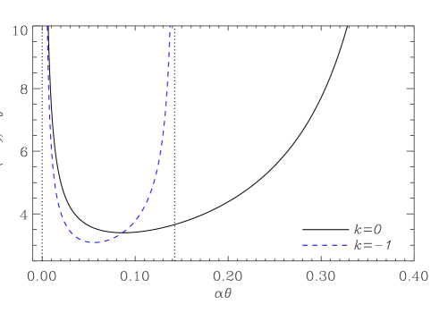
Figure 1: Scale factors as functions of the parameter $\alpha\theta$ for two cases of interest, described by Eq. (44) in the case derived in Sec. II, i.e. with $\omega=-3$. The flat case is shown as the full line, whereas the open case is plotted as a dashed line. For these figures, the parameters have been chosen to be $M=1.1$ and $C=1$. The straight dotted line at $\alpha\theta\sim 0.142$ represents the maximal permitted value for the timelike coordinate $\alpha\theta$, i.e. it corresponds to the future infinity, in the open case $k=-1$, the equivalent line for the flat case $k=0$ being at the edge of the figure (i.e. the allowed range of variation is in this case $0\leq\alpha\theta\mathrel{\hbox to0.0pt{\lower 3.0pt\hbox{$\mathchar 536\relax$}\hss}\raise 2.0pt\hbox{$\mathchar 316\relax$}}0.4$).

In what follows, we sketch an analysis of the problem of violation of the energy conditions, adapting the expressions for the nonminimal coupling with the dilatonic field. The effective energy density $\rho_{\mathrm{eff}}$ and pressure $p_{\mathrm{eff}}$ are derived from the field equations (8), whose right-hand side we take to be the effective stress-energy tensor $T^{\mu\nu}_{\mathrm{eff}}$ we are looking for, assuming an Einstein-like form for Eq. (8) as

$$R_{\mu\nu}-\frac{1}{2}g_{\mu\nu}R=8\pi G_{{}_{\rm N}}T_{\mu\nu}^{\mathrm{eff}}.$$ (57)

The corresponding cosmological equations are then seen as projections of Eq. (57) by means of a normalized timelike vector $u_{\mu}$ (with $u_{\mu}u^{\mu}=1$): defining $\rho_{\mathrm{eff}}=T^{\mu\nu}_{\mathrm{eff}}u_{\mu}u_{\nu}$ and $p_{\mathrm{eff}}=-\frac{1}{3}T^{\mu\nu}_{\mathrm{eff}}\left(g_{\mu\nu}-u_{\mu}u_{\nu}\right)$, Eqs. (8) are then nothing but the usual system describing a cosmological background with a fluid.

Starting with the field equations derived above, one obtains the following expressions:

$$8\pi G_{{}_{\rm N}}\rho_{\mathrm{eff}} = \frac{8\pi}{\phi}\rho+\frac{\omega}{2}\frac{\dot{\phi}^{2}}{\phi^{2}}+\frac{1}{2}\frac{\dot{\Psi}^{2}}{\phi^{2}}+\frac{1}{2}\frac{\dot{\xi}^{2}}{\phi}$$ (58)

$$-3\frac{\dot{a}}{a}\frac{\dot{\phi}}{\phi},$$

$$8\pi G_{{}_{\rm N}}p_{\mathrm{eff}} = \frac{8\pi}{3\phi}\rho+\frac{\omega}{2}\frac{\dot{\phi}^{2}}{\phi^{2}}+\frac{1}{2}\frac{\dot{\Psi}^{2}}{\phi^{2}}+\frac{1}{2}\frac{\dot{\xi}^{2}}{\phi}$$ (59)

$$+\frac{\ddot{\phi}}{\phi}+2\frac{\dot{a}}{a}\frac{\dot{\phi}}{\phi},$$

which, contrary to the standard cosmological situation, are both not positive definite. The energy conditions may therefore be violated, due to the terms arising from the nonminimal coupling and if either $\omega$ or $\phi$ is negative.

To understand the causes for the bounces in our solutions, it is also useful to use Eq. (25). In the normal cases (from the purely mathematical point of view) with nonvanishing dilaton, we have seen that one must have $\phi<0$ (repulsive gravity) in order to have a bounce. In this case, the negative dilaton is sufficient to make the bounce, and there is no need to have $\omega<0$. In the normal cases with the dilaton vanishing at some point, $b$ does not actually bounce. Hence the dilaton $\phi$ can be positive. The bounce then comes from the requirement $\omega<0$.

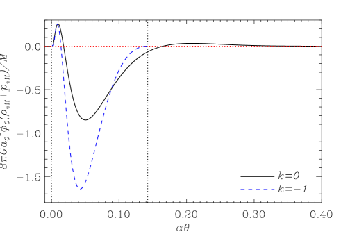
Figure 2: The null energy condition during the evolution of the Universe models depicted in Fig. 1, again with the full line standing for the $k=0$ case (rescaled by a factor of $3$ to appear with comparable magnitude) and the dashed line for $k=-1$.

In the anomalous cases, where the dilaton is strictly positive and finite, it is the negative value of $\omega$, more precisely the fact that $\omega<-3/2$, which causes the bounces. Figure 1 illustrates two cases of bounces for which the scale factors are shown, taken in the anomalous axionic case, i.e. using the solution (44). In terms of the scale factor, the expression for the null energy condition reads

$$8\pi G_{{}_{\rm N}}\left(\rho_{\mathrm{eff}}+p_{\mathrm{eff}}\right)=\frac{2}{a^{6}}\left[4\left(\frac{a^{\prime}}{a}\right)^{2}-\frac{a^{\prime\prime}}{a}+ka^{4}\right],$$ (60)

which coincides, on shell, with what is obtained by summing Eqs. (58) and (59). Plotting the right hand side of this expression as in Fig. 2 for the cases of Fig. 1, we verify that the null energy condition can be violated in large domains around the bounce, depending on the choice of parameters. One should notice that the timelike coordinate $\theta$ has been chosen to emphasize the bounce itself. In terms of the cosmic time, the domain where the NEC is violated is in fact reduced to just a small fraction of the whole interval, since the latter is actually infinite. Moreover, no violation is observed in the large positive time limit, where the models tend to Milne or radiation dominated universes.

V Conclusions

We have constructed fully regular cosmological solutions in the framework of effective actions derived from string theory principles. These solutions present bouncing behaviors for a wide range of parameters ($\omega<-3/2$), and are singularity free; furthermore, the spacetimes they lead to are geodesically complete, thereby improving the so-called horizon problem of standard cosmology. Stemming from string theory in the context of the so-called $F$ theory in twelve dimensions, where it is possible to have $\omega<-3/2$, they have a reasonably sound basis as long as the dilaton is strictly positive and finite in such a case. As a consequence, it is not necessary to go beyond the tree level approximation in any part of their histories: the analytic solutions exhibited above can describe the whole history of the cosmological models they represent. Their consequences may, in turn, be used as cosmological tests.

Remembering that the radiation fluid included here also has a motivation in the superstring type IIB action, this turns out to be, to our knowledge, the first case where a complete regular bouncing cosmological solution is obtained in the string framework and related theories, which moreover is smoothly connected with the standard cosmological model radiation dominated phase. This solution may have flat or negative curvature spatial sections.

In the axionic and RR cases with $k=0$ or $k=-1$, there are nonsingular bouncing solutions for $-3/2<\omega<-4/3$ but with vanishing dilaton in the beginning, where the tree level action cannot be trusted, and bouncing solutions with an initial curvature singularity if $-4/3<\omega<0$. If $k=-1$ and $-3/2<\omega<0$ (normal, including the pure string case), one can have singularity free bouncing solutions with, however, a negative definite dilaton field.

As all the models with $\omega<-3/2$ have the interesting feature to approach flat spacetime in the infinite past (either in Milne coordinates for $k=-1$, or the infinitely large radiation dominated standard model with $k=0$), there is the possibility to implement a quantum spectrum of perturbations in the initial asymptotics without any trans-Planckian problem [20], and, at the same time, to accomplish a smooth transition to the standard cosmological model when, after the bounce, a standard radiation dominated phase is recovered (asymptotically in the $k=0$ case), preserving some of its main achievements like, e.g. primordial nucleosynthesis. The bouncing solutions with $\omega>-3/2$ and positive dilaton still present some sort of trans-Planckian problem as long as the string expansion parameter diverges initially and one must go beyond the tree level action in such cases.

Notice that, in the cases where the dilaton is strictly positive, the initial value of the dilatonic field can be made smaller than its final value. Hence, the gravitational coupling can be initially given a much greater value than it would have today. This opens the possibility to solve the hierarchical problem of the gravitational coupling, in a spirit similar to the so-called brane cosmology [21].

- [1] J. Polchinski, String theory, Cambridge University Press (Cambridge, 1998), Vols. I & II.
- [2] M. B. Green, J. H. Schwarz, and E. Witten, Superstring theory, Cambridge University Press (Cambridge, 1987), Vols. I & II.
- [3] E. Kiritsis, “Introduction to superstring theory”, hep-th/9709062.
- [4] N. Khviengia, Z. Khviengia, H. Lu, and C. N. Pope, Class. Quantum Grav. 15, 759 (1998).
- [5] I. Antoniadis, N. Arkani-Hamed, S. Dimopoulos, and G. Dvali, Phys. Lett. B 436, 257 (1998); L. Randall and R. Sundrum, Phys. Rev. Lett. 83, 4690 (1999).
- [6] G. Veneziano, Phys. Lett. B 265, 287 (1991); M. Gasperini and G. Veneziano, Astropart. Phys. 1, 317 (1993); see also J. E. Lidsey, D. Wands, and E. J. Copeland, Phys. Rep. 337, 343 (2000); G. Veneziano, String Cosmology : The Pre-Big Bang Scenario, Les Houches summer school, edited by P. Binétruy et al. (Elsevier Science Publishers, 2001); M. Gasperini and G. Veneziano, Phys. Rep. 373, 1 (2003).
- [7] P. Binétruy, C. Deffayet, and P. Peter, Phys. Lett. B 441, 52 (1998).
- [8] P. Peter and N. Pinto-Neto,Phys. Rev. D66, 063509 (2002).
- [9] J. C. Fabris, P. Peter, and N. Pinto-Neto (in preparation).
- [10] J. E. Lidsey, D. Wands, and E. J. Copeland, Phys. Rep. 337, 343 (2000).
- [11] A. Feinstein and M. A. Vazquez-Mozo, Nucl. Phys. B568, 405 (2000).
- [12] C. P. Constantinidis, J. C. Fabris, R. G. Furtado, and M. Picco, Phys. Rev. D61, 043503 (2000).
- [13] K. A. Bronnikov and J. C. Fabris, J. High Energy Phys. 09, 62 (2002); see also S. Tsujikawa, hep-th/0302181 where other solutions are also discussed.
- [14] R. Brandenberger, R. Easther, and J. Maia, J. High Energy Phys. 08, 007 (1998); D. A. Easson and R. H. Brandenberger, ibid. 09, 003 (1999).
- [15] J. C. Fabris, Phys. Lett. B 267, 30 (1991).
- [16] P. Peter and N. Pinto-Neto, Phys. Rev. D65, 023513 (2001), and references therein.
- [17] I. S. Gradshteyn and I. M. Ryshik, Table of Integrals, Series and Products, (Academic Press, New York, 1980).
- [18] C. Molina-Paris and M. Visser, Phys. Lett. B 455, 90 (1999); see also R. Brustein and R. Madden, ibid. 410, 110 (1997); Phys. Rev. D57, 712 (1998); N. Kaloper, R. Madden, and K. A. Olive, Nucl. Phys. B452, 667 (1995); Phys. Lett. B 371, 34 (1996); R. Easther, K. Maeda, and D. Wands, Phys. Rev. D53, 4247 (1996); J. Khoury, B. A. Ovrut, N. Seiberg, P. J. Steinhardt, and N. Turok, ibid. 65, 086007 (2002).
- [19] S. W. Hawking and G. F. R. Ellis, The Large Scale Structure of Space-time (Cambridge University Press, Cambridge, England, 1973); R. M. Wald, General Relativity (Chicago University Press, Chicago, 1984); see also A. Borde and A. Vilenkin, Phys. Rev. D56, 717 (1997) for a more recent discussion.
- [20] J. Martin and R. Brandenberger, Phys. Rev. D63, 123501 (2001); R. Brandenberger and J. Martin, Mod. Phys. Lett. A 16, 999 (2001); J. C. Niemeyer, Phys. Rev. D63, 123502 (2001).
- [21] D. Langlois, in Proceedings of the YITP workshop on ”Braneworld - Dynamics of spacetime boundary” [Prog. Theor. Phys. Suppl. 148, 181 (2003)].