Remarks on Charged Vortices in the Maxwell-Chern-Simons Model

Abstract

We study vortex-like configuration in Maxwell-Chern-Simons Electrodynamics. Attention is paid to the similarity it shares with the Nielsen-Olesen solutions at large distances. A magnetic symmetry between a point-like and an azimuthal-like current in this framework is also pointed out. Furthermore, we address the issue of a neutral spinless particle interacting with a charged vortex, and obtain that the Aharonov-Casher-type phase depends upon mass and distance parameters.

I Introduction

Since the appearance of the first works on field-theoretic models defined in the (2+1)-dimensional space-time, nearly two decades ago firstones1 ; firstones2 ; reviewsWDK ; Dunne , a great deal of efforts has been driven to the subject GFT . Actually, planar physics has not only shed light on theoretical questions concerning the structure and topology of such a space-time, but has also provided a number of new and powerful ideas and techniques with wide applications, for example, in Condensed Matter phenomena. “Exotic objects” exhibiting fractional statistics and charge, for instance, have been proposed as the keystone entities for a better and deeper understanding of the Fractional Quantum Hall Effect (for details, see Ref. fqhe ). Along this line, there is also a broad literature claiming for their importance in a number of mechanisms involved in the so-called High-Tc Superconductivity, whenever planar physical effects cannot be neglected (for reviews, see Ref. htcsup ).

In this sense, the so-called Chern-Simons action is a simple and good example of a model which provides such requirements. This comes about by virtue of its topological nature, which gives rise to a number of novelties, whenever coupled to matter or even to other models. Actually, besides the fractional statistics, such an action also displays the interesting feature of providing a gauge invariant mass gap for matter and gauge fields (for further details, see Ref. firstones2 ). In this case, the excitations described by the matter fields are shown to be attached to the magnetic vortex-like objects. As a consequence of the connection between an Aharonov-Bohm type phase and quantum physics, these composite objects display fractional statistics anyons ; reviewsWDK ; Dunne ; htcsup .

   In a recent paper, we have studied issues concerning planar radiation in Maxwell and Maxwell-Chern-Simons (MCS) models, namely, how the Huyghens Principle and Planck’s Law read in the planar world pla . A number of results have indicated that “planar photons” should behave quite different from their (3+1)-dimensional counterparts. In this sense, the present work may be viewed as a step forward in the issue of planar radiation propagation. Indeed, Section 4 is devoted to the Aharonov-Casher-type effect between a MCS charged vortex and a neutral spinless particle. In this case, the results may be considered as a way to measure the Chern-Simons parameter, as long as experiments concerning planar aspects of physical radiation could be performed.

II The MCS vortex-like configuration

Let us start off with the pure Chern-Simons model, which may be written as:

$$\mathcal{L}_{\mathrm{CS}}=\frac{m}{2}\epsilon^{\mu\nu\kappa}\,A_{\mu}\partial_{\nu}A_{\kappa}-A_{\mu}j^{\mu}\,,$$ (1)

where $j^{\mu}$ is the conserved current, $\partial_{\mu}j^{\mu}=0$. The equations of motion are simply:

$$F_{\mu\nu}=\frac{1}{m}\epsilon_{\mu\nu\kappa}j^{\kappa}\,,$$ (2)

while Bianchi identity reads: $\partial_{\mu}\widetilde{F}^{\mu}=0$; with the usual definitions: $F_{\mu\nu}=\partial_{\mu}A_{\nu}-\partial_{\nu}A_{\mu}$ and $\widetilde{F}^{\mu}=\frac{1}{2}\epsilon^{\mu\nu\kappa}F_{\nu\kappa}$. Now, if we take a point-like electric charge, $\rho(\vec{x})=q\delta^{2}(\vec{x})$, then we get a point-like magnetic vortex, $B(\vec{x})=(q/m)\delta^{2}(\vec{x})$ attached to the charge. This vortex has finite flux, $\Phi_{B}=\int\,d^{2}\vec{x}\,B(\vec{x})=q/m$, but the magnetic energy, $\mathcal{E}_{B}=\frac{1}{2}\int\,d^{2}\vec{x}\,B^{2}(\vec{x})$, blows up, highlighting its point-like structure. In addition, we should notice that, in this framework, electromagnetic interaction takes place only by “contact”, since there is no photon dynamics. Then, whenever two (or more) of these composites (charged vortex) interact amongst themselves, topological phases (Aharonov-Bohm type) are induced in one another, and fractional statistics takes place (some reviews on the subject are listed in Refs. reviewsWDK ; Dunne ).

On the other hand, whenever Higgs fields are coupled to Chern-Simons Lagrangian density, i.e.:

$$\mathcal{L}_{\mathrm{CSH}}=\frac{m}{2}\epsilon^{\mu\nu\kappa}\,A_{\mu}\partial_{\nu}A_{\kappa}+|D_{\mu}\phi|^{2}-V(\phi)\,,$$ (3)

then, the eqs. of motion (for the $A_{\mu}$-field) take the forms:

$$F_{\mu\nu}=\frac{1}{m}\epsilon_{\mu\nu\kappa}j^{\kappa}=\frac{i}{m}\epsilon_{\mu\nu\kappa}\left[\phi^{*}\,D^{\kappa}\phi-(D^{\kappa}\phi)^{*}\,\phi\right]\,,$$ (4)

while Bianchi identity remains $\partial_{\mu}\widetilde{F}^{\mu}=0$. The magnetic field, for example, now reads:

$$B(x)=\frac{i}{m}\left[\phi^{*}\,D_{0}\phi-(D_{0}\phi)^{*}\,\phi\right]\,.$$ (5)

The magnetic vortex-like configurations associated to the solution above are electrically charged (like those appearing in pure CS model), in contrast with their counterparts of the usual Abelian Higgs model. Moreover, it is well-known that such a model supports topological ($|\phi|\to\nu$ as $|\vec{x}|\to\infty$) and non-topological ($|\phi|\to 0$ as $|\vec{x}|\to\infty$) solitons, as well. Their flux, charge and energy are respectively given by:

$$\hskip-28.45274pt\Phi_{B}=2\pi N\,,\quad Q=m\Phi_{B}\quad\mathrm{and}\quad\mathcal{E}=\nu^{2}|\Phi_{B}|\,,$$ (6)

$$\hskip-28.45274pt\Phi_{B}=2\pi(N+\alpha)\,,\quad Q=m\Phi_{B}\quad\mathrm{and}\quad\mathcal{E}=\nu^{2}|\Phi_{B}|,$$ (7)

with integer $N$, measuring the vorticity of the soliton solutions, while $\alpha$ is a continuous parameter. Notice also that all of these three quantities are finite. Namely, the finiteness of the energy implies that such configurations are finite-size (for a review, see Ref. Dunne and related references therein).

In the present work, we would like to concentrate on the Maxwell-Chern-Simons Electrodynamics, whose Lagrangian density reads as below:

$$\mathcal{L}_{\mathrm{MCS}}=-\frac{1}{4}F_{\mu\nu}F^{\mu\nu}+\frac{m}{2}\epsilon^{\mu\nu\kappa}\,A_{\mu}\partial_{\nu}A_{\kappa}-A_{\mu}j^{\mu}\,,$$ (8)

which leads us to the following eqs. of motion:

$$\left(\partial_{\nu}\partial^{\nu}+m^{2}\right)\widetilde{F}^{\mu}=\frac{1}{m}\epsilon^{\mu\nu\kappa}\partial_{\nu}j_{\kappa}-j^{\mu},$$ (9)

besides the geometric one, $\partial_{\mu}\widetilde{F}^{\mu}=0$.

By virtue of the Maxwell term, Gauss Law becomes a dynamical equation, and interaction between electric charges turns out to be of finite range. As we shall see in what follows, such a feature is responsible for another very interesting aspect concerning solutions of the $\vec{E}$ and $B$ fields, specially the magnetic sector, which now appears to have associated finite-energy.

For that, let us consider eq. (9), describing a point-like electric charge, $j_{0}=\rho(\vec{x})=q\delta^{2}(\vec{x})$, integrated over the two-dimensional volume. Then, we get (using that the classical fields, $\vec{E}$ and $B$ are short-range; a more general study of this problem, including time-dependent solutions, may be found in Ref. prd63 ):

$$\int_{V}\,d^{2}\vec{x}\,\nabla\cdot\vec{E}=\oint_{\partial V}\vec{E}\cdot d\vec{S}\mid_{r\to\infty}=0=q-m\Phi_{B}\,,$$ (10)

which implies that the total magnetic flux associated to the $B$-field is:

$$\Phi_{B}=\int_{V}\,B(x)d^{2}\vec{x}=\frac{q}{m}\,,$$ (11)

and the total electric flux vanishes.

Let us now seek for possible solutions to the eq. (11). An immediate solution consists in taking the magnetic field concentrated at a unique point (like in the pure Chern-Simons case): $B(\vec{x})=\frac{q}{m}\delta^{2}(\vec{x})$. It is easy to check that, while this field satisfies (11), it does violate Gauss Law, $\nabla\cdot\vec{E}(\vec{x})=\rho(\vec{x})-mB(\vec{x})$, whenever $\nabla\cdot\vec{E}\neq 0$. Actually, the suitable solution for the magnetic and electric fields which satisfy the eqs. (9), (10) and (11) are given by:

$$B(\vec{x}) = +\frac{mq}{2\pi}\,K_{0}\left(m|\vec{x}|\right)\,,$$ (12)

$$\vec{E}(\vec{x}) = +\frac{mq}{2\pi}\,K_{1}\left(m|\vec{x}|\right)\hat{\mathbf{x}}\,.$$ (13)

Here, $K_{0}$ and $K_{1}$ are modified Bessel functions of 2nd kind and $\hat{\mathbf{x}}=\vec{x}/|\vec{x}|$.

The gauge potential, in turn, appears to be:

$$A^{0}(\vec{x})=+\frac{q}{2\pi}\,K_{0}(m|\vec{x}|)\,,$$ (14)

$$A^{i}(\vec{x})=+\frac{q}{2\pi m}\epsilon^{ij}\frac{x_{j}}{|\vec{x}|}\left(\frac{1}{|\vec{x}|}-m\,K_{1}(m|\vec{x}|)\right).$$ (15)

Now, let us remark that, since $K_{0}$ and $K_{1}$ behave like $e^{\sqrt{m|\vec{x}|}}/\sqrt{m|\vec{x}|}$ as $|\vec{x}|\to\infty$, then $\vec{E}$, $B$ and $A^{0}$ vanish asymptotically. In contrast, the vector potential is long-range: $A^{i}(\vec{x})=+\frac{q}{2\pi m}\epsilon^{ij}\frac{x_{j}}{|\vec{x}|^{2}}$ as $|\vec{x}|\to\infty$, which is a pure-gauge term, $\partial^{i}\theta(\vec{x})$, and supports, similarly to the pure Chern-Simons case, the magnetic vortex-like solutions, eq. (12). Another interesting feature of such quantities concerns their behavior near the origin: while $\vec{E}$, $B$ and $A^{0}$ blow up as $|\vec{x}|\to 0$, the vector potential, $\vec{A}$, vanishes. Then, although CS Electrodynamics quantities are recovered at large distances (what is equivalent to take $m\to\infty$, as usual), the finite scale behavior of both models are quite different, mainly as $|\vec{x}|\to 0$.

The magnetic field of eq. (12) presents finite flux and energy given respectively by (see expressions 6.561-16 in page 684, and 5.54-2 in page 634 of the Ref. grad1 ):

$$\Phi_{B} = \frac{q}{m},$$

$$\mathcal{E}_{B} = \frac{q^{2}m^{2}}{8\pi^{2}}\int d^{2}\vec{x}\biggl{[}K_{0}(m|\vec{x}|)\biggr{]}^{2}=\frac{q^{2}}{8\pi},$$

which could suggest that our electrically charged magnetic vortex-like configuration, (12), presents finite-size. However, since magnetic vortices in MCS framework always appear electrically charged, then their total energy (electric + magnetic) blows up, since solution (13) leads to a divergent electric energy. Then, although the magnetic sector presents finite energy, the charged vortices are structure-less, similarly to their counterparts in pure Chern-Simons model.

To end this section, let us perform a brief comparison amongst our magnetic results and those found by Nielsen and Olesen NO in the case of the (3+1)-dimensional Abelian Maxwell-Higgs (AMH) model with axial-symmetry (then, an effective (2+1)d theory). Their asymptotic results read as below:

$$|\vec{A}(\vec{x})|_{\mbox{{\tiny N-O}}}=\frac{1}{er}-|\phi|\,K_{1}(e|\phi|r)\,,$$ (16)

$$|\vec{B}(\vec{x})|_{\mbox{{\tiny N-O}}}=+\,e|\phi|^{2}\,K_{0}(e|\phi|r)\,,$$ (17)

where $e$ is the minimal coupling constant, $D_{\mu}=\partial_{\mu}+ieA_{\mu}$, while $|\phi|={\mbox{\rm constant}}$ is the absolute value of the Higgs field as $r$ becomes large.

Since their results and ours are strictly obtained in different space-times, then the gauge potential and the classical electromagnetic fields have different canonical dimensions. So, at a first stage, only the arguments of the Bessel functions could be compared. In this case, the similarity in behavior demands that:

$$m=e|\phi|,$$

which states us that the CS-parameter is fixed by the value of the Higgs field (times the constant $e$).

Nevertheless, Nielsen-Olesen solutions, eqs. (16,17), are strictly valid whenever AMH model is defined in (2+1) dimensions. Now, the gauge coupling constant and the Higgs field possess the same canonical dimension, $[e]=[\phi]=[\mathrm{mass}]^{1/2}$ (even though a $\phi^{6}$ -type potential be included). In such a scenario, a “complete identification” amongst $\vec{A}_{\mbox{{\tiny N-O}}}$, $B_{\mbox{{\tiny N-O}}}$ and expressions (12-15) may be carried out, provided that the following constraints hold:

$$m=e|\phi|=\frac{eq}{2\pi}\,.$$ (18)

If we now take into account that the electric charge appears as multiple of the elementary one, $q=n\,e$ ($n$ integer) then, we finally have that:

$$\frac{2\pi m}{e^{2}}=\frac{|\phi|}{e}=n\,.$$ (19)

Even though the relation above could not be considered as a Dirac-like quantization condition for the mass parameter (or Higgs field) in (2+1)-dimensional Abelian Electrodynamics, since no quantum mechanics was involved, it is interesting to remark that expression (19) fixes the possible values of $m$ (and/or $|\phi|$), in those regimes in which (2+1)-dimensional AMH and MCS models present the same physical behavior, whenever $|\phi|$ takes a constant value (see however, Refs.HTetc , dealing with some cases in which the topological mass parameter appears to be quantized). Then, we may also conclude that the magnetic sector of the non-linear AMH model behaves as if it were a linear one, as long as distances become very large (and $|\phi|\to\mathrm{constant}$).

III Magnetic Symmetry between Charges and Azimuthal Currents

Let us again consider eq. (9), in which the source is now taken tobe a steady and azimuthal electric current, say $j_{i}=Q\epsilon_{ij}\,x_{j}/2\pi|\vec{x}|^{2}$; $\rho=0$. The electric and magnetic fields associated with such a configuration read:

$$\vec{E}(\vec{x}) = \frac{Q}{2\pi\,m}\frac{\vec{x}}{|\vec{x}|}\left(\frac{1}{|\vec{x}|}-m\,K_{1}(m|\vec{x}|)\right)\,,$$ (20)

$$B(\vec{x}) = -\frac{Q}{2\pi}K_{0}(m|\vec{x}|)\,.$$

Notice that the $B$ above exactly coincides with (12), whenever $Q=-qm$, which states us that we have a magnetic symmetry between a point-like charge and such a electric current. It should be mentioned that a similar scenario does not hold, for example, neither for the pure Maxwell nor the Chern-Simons models. Notice also that both fields yield finite flux. The magnetic energy is also finite while the electric one presents infrared and ultraviolet divergences.

Another interesting point here is that, if we introduce a cutoff in the current above:

$$j_{i}(\vec{x})=\left\{\begin{array}[]{l}0\qquad\qquad\mathrm{if}\quad|\vec{x}|<r_{0}\\ \\ \frac{{Q}}{2\pi}\frac{\epsilon_{ij}\,x_{j}}{|\vec{x}|^{2}}\quad\mathrm{if}\quad|\vec{x}|>r_{0}\,,\end{array}\right.$$ (24)

then $r_{0}$ will be naturally fixed by the Chern-Simons parameter, as we shall see in what follows.

Nevertheless, before that, let us explain what we mean by the expression above. For that, consider a very thin finite-size sample placed in a region where a perpendicular magnetic field of strength $B_{0}$, crosses it. In addition, suppose, for simplicity, that such a field could be confined to a very small disc (of radius $r_{0}$) around a given point in the sample. Then, an electric current looking like (24) would appear in the sample. To some extent, this scenario could be taken as an analogue to the presence of a unique neutral magnetic vortex inside a high-Tc superconducting sample (an Aharonov-Bohm-type flux) surrounded by such an external current. The solutions to the eq. (9) associated to the current above read as below:

$$\begin{array}[]{l}B(\vec{x})=B_{0}\,I_{0}(m|\vec{x}|)\,,\\ \hskip 136.5733pt\mathrm{if}\quad|\vec{x}|<r_{0},\\ \vec{E}(\vec{x})=B_{0}\,I_{0}(m|\vec{x}|)\hat{\mathbf{x}}\,,\\ \end{array}$$ (28)

$$\begin{array}[]{l}\hskip-17.07182ptB(\vec{x})=-\frac{{Q}}{2\pi}\,K_{0}(m|\vec{x}|)\,,\\ \hskip 128.0374pt\quad\mathrm{if}\quad|\vec{x}|>r_{0},\\ \hskip-17.07182pt\vec{E}(\vec{x})=\frac{{Q}}{2\pi m}\left(\frac{1}{|\vec{x}|}-mK_{1}(m|\vec{x}|)\right)\hat{\mathbf{x}}.\end{array}$$ (32)

In addition, the scalar potentials associated to the solutions above read respectively, as follows:

$$\hskip-28.45274ptA_{0}(\vec{x})=\frac{B_{0}}{m}I_{0}(m|\vec{x}|),\qquad\qquad\qquad\quad\;\mathrm{if}\,|\vec{x}|<r_{0}\,,$$ (33)

(34)

$$\hskip-28.45274ptA_{0}(\vec{x})=-\frac{{Q}}{m}\left(\ln(m|\vec{x}|)+K_{0}(m|\vec{x}|)\right),\;\;\mathrm{if}\,|\vec{x}|>r_{0}\,,$$

while the vector potential takes the forms below:

$$\hskip-28.45274ptA^{i}(\vec{x})=\frac{B_{0}}{m}I_{0}(m|\vec{x}|)\epsilon^{ij}\,\frac{x^{j}}{|\vec{x}}|\qquad\qquad\qquad\;\mathrm{if}\,|\vec{x}|<r_{0}\,,$$ (35)

(36)

$$\hskip-28.45274ptA^{i}(\vec{x})=-\frac{{Q}\epsilon^{ij}\,x^{j}}{2\pi m^{2}|\vec{x}|}\left(\frac{1}{|\vec{x}|}-mK_{1}(m|\vec{x}|)\right),\;\mathrm{if}\,|\vec{x}|>r_{0},$$

where $I_{0}$ is the modified Bessel functions of 2nd kind. Notice the similarity between the scalar and vector quantities above, namely, observe that the electric field is dual to the vector potential (up to the multiplicative constant $m$).

In order that the solutions above make sense, the expressions for the scalar potential should be continuous at the “effective vortex radius”, $|\vec{x}|=r_{0}$. This condition leads us to the following set of equations:

$$B_{0}\,I_{0}(mr_{0})=-\frac{{Q}}{2\pi}K_{0}(mr_{0})\,,$$ (37)

$$\frac{B_{0}}{m}\,I_{0}(mr_{0})=-\frac{{Q}}{2\pi m}\biggl{(}\,\ln(mr_{0})+K_{0}(mr_{0})\,\biggr{)}\,,$$ (38)

which can be simultaneously satisfied if and only if $r_{0}=1/m$. This amounts to saying that an eddy-like current around a neutral vortex, in the MCS framework, naturally fixes the radius of the latter as being the inverse of the CS parameter (value identical to that obtained in pure CS model for its charged vortex; see Ref. Jackiwvortex , for details). Furthermore, we also obtain that the strength of the eddy current increases, as an external magnetic field is brought about, and vice-versa; this means: $|{Q}|=2\pi B_{0}\frac{I_{0}(1)}{K_{0}(1)}\approx 6\pi B_{0}$. [Figure 1 shows how the magnetic field above behaves “inside” and “outside” this vortex. We have taken $r_{0}=1$ and $B_{0}=1$].

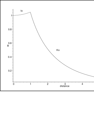
Figure 1: The behavior of the magnetic field, $B(r)$, inside the vortex ($r_{0}<1$) and outside ($r_{0}>1$). We have taken $r_{0}=B_{0}=1$ and centered the vortex at the origin.

IV Neutral Spinless Particle, Charged Vortices and the Aharonov-Casher Effect

As it is well-known, in (2+1) dimensions, even spinless particles may carry anomalous magnetic momenta (AMM), whenever they interact with an electromagnetic field. The reason for this peculiarity lies in the fact that the canonical momentum of particles can naturally be supplemented by the dual of $F_{\mu\nu}$, by means of a non-minimal coupling as follows:

$$p_{\mu}\quad\longrightarrow\quad p_{\mu}+f\widetilde{F}_{\mu}\,,$$ (39)

where the constant $f$ measures the planar AMM of the particle (see Ref. nonminimal ; see also Refs. prd65 ; CK ; Hagen ).

Now, let us recall that the field-strength generated by a charged vortex in MCS framework reads like eqs. (12-13):

$$\widetilde{F}^{\mu}=(-B;\epsilon^{ij}E^{i}\hat{{x}}^{j})=\frac{mq}{2\pi}\biggl{[}K_{0}(mr);\epsilon^{ij}\hat{{x}}^{j}\,K_{1}(mr)\biggr{]}.$$ (40)

Thus, for a neutral spinless particle (of mass M) which experiences the fields above, its energy will be given by (the case of spin particles may be carried out in an analogous way):

$$\mathbf{H}=+\frac{1}{2M}\left(p_{\mu}+f\widetilde{F}_{\mu}\right)^{2}\,.$$ (41)

Indeed, since its free wave-function ($f=0$) satisfies the free Schrödinger equation, $[2i\,\hbar\,M\partial_{t}+\nabla^{2}]\psi^{0}(\mathbf{x},t)=0$, then WKB approximation will lead us to (hereafter, we write $\hbar$ constant explicitly):

$$\psi(\mathbf{x},t)=\psi^{0}(\mathbf{x},t)\,exp\left[-i\hbar f\int\,dx_{\mu}\widetilde{F}^{\mu}\right]\,.$$ (42)

Here, we clearly realize that the non-minimal prescription, (39), is equivalent (at WKB level) to introducing a non-integrable phase to $\psi^{0}$. Now, the interesting case to be considered regards the particle performing a spatial loop, $\theta$, in an adiabatic way around the charged vortex. In such a case, we have:

$$\theta=f\oint\,dx_{i}\,\widetilde{F}^{i}=f\oint_{C}\,\vec{E}\cdot d\vec{x}=f\Phi_{E}\,.$$ (43)

Now, using that $\oint_{C}\,\vec{E}\cdot d\vec{x}=\int_{S}\,\nabla\cdot\vec{E}\,d^{2}\vec{x}=\int_{S}d^{2}\vec{x}\left[q\,\delta^{2}(\vec{x})\,-mB\right]$, we get:

$$\theta=f\Phi_{E}=f(q-m\Phi_{B})\,.$$ (44)

The point to be stressed is that the electric or the magnetic flux above is not the total flux, but only that part contained inside a circular region of radius $R$ ($R$ is the distance between the MCS vortex and the neutral particle). This flux is given by (see formula 6.561-8 on page 683, in Ref. grad1 ):

$$\Phi_{B}=qm\int^{R}_{0}\,rK_{0}(mr)\,dr=\frac{q}{m}\biggl{[}1-mR\,K_{1}(mR)\biggr{]}\,.$$

Finally, we obtain that the Aharonov-Casher phase is given as below:

$$\theta_{AC}=\hbar fq\,mR\,K_{1}(mR)\,,$$ (45)

which implies that $\psi(\mathbf{x},t)=\psi^{0}(\mathbf{x},t)\,e^{i\theta_{AC}}$. Therefore, the wave-function describing the neutral spinless particle acquires a topological phase that depends upon mass and distance parameters, as previously announced (see also Fig. 2). The pure Maxwell limit, $m\to 0$ (or equivalently, $R\to 0$), taken in this phase, yields the result obtained by Carrington and Kunstatter CK , namely, $\theta_{AC}|_{m\to 0}=\hbar fq$. On the other hand, as $m\to\infty$ (pure CS limit) then $\theta_{AC}$ vanishes. This result agrees with Gauss law in MCS framework and also with the fact that in pure CS framework there is no static electric field, yielding $\Phi_{E}\equiv 0$ everywhere in this case.

Concerning the limit discussed above, let us recall that the energy density radiated, per unity of frequency, for “planar photons” in thermal equilibrium, $U^{\rm 2+1}(\nu^{\prime},m)$, is vanishing, whenever it is taken in the planar version of the Planck’s Law pla . Then, we may conclude that, when the dynamics is switched off, the same occurs with $U^{\rm 2+1}(\nu^{\prime},m)$. Indeed, a similar scenario seems to take place here, since if $m\to\infty$, so does $\theta_{AC}$. This is interesting because such a phase has topological origin, but as long as dynamics is turned off the phase vanishes.

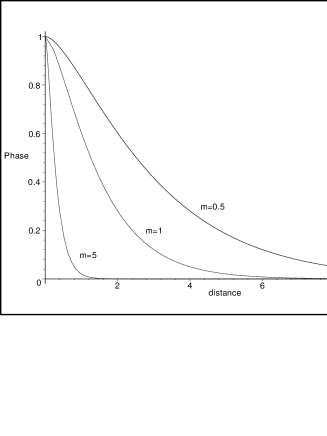
Figure 2: The Aharonov-Casher phase, as function of distance, is exhibited for some values of the Chern-Simons parameter.

Notice also that, by virtue of the connection between spin and quantum statistics, then the neutral particle formerly taken to be spinless, could now display non-trivial statistics, namely fractional spin.

As a final remark, we mention that, since actual experiments would deal with finite values for $R$ and $m$, then our present result, (45), suggests a way to determine the Chern-Simons parameter (as long as $q$ and $f$ are known), whenever one could provides conditions such that the experiments are able to take into account planar effects on the quantum radiation.

V Conclusions and Prospects

Chern-Simons Electrodynamics naturally associates a point-like magnetic flux to each (point-like) electric charge. Whenever a Maxwell term is taken into account, leading to the MCS model, the magnetic sector presents finite energy, despite the lack of structure of the composite object. In addition, we have pointed out that, in the MCS framework, the magnetic field created by a static point-like charge is identical to that generated by an azimuthal-like steady current. Moreover, if we consider a ‘ neutral magnetic vortex’ surrounded by such a current (like those eddy-current around magnetic fluxons observed in High-T_c superconductors) the vortex radius is fixed to be exactly $r_{0}=1/m$. A comparison between our magnetic configurations and those obtained by Nielsen and Olesen NO was also performed at large distances, where they were seen to present analogous behavior, provided that a relation between the Chern-Simons parameter and the Higgs field is implemented.

We have also seen that, whenever a neutral spinless particle interacts with an MCS charged composite vortex, the Aharonov-Casher (AC) effect is induced in the former, as expected. The novelty found here is that such a topological phase depends upon mass and distance between the spinless particle and the vortex. Furthermore, as $m\to 0$, we recover the usual result known in the literature CK .

Our results concern photons as if they were planar excitations, possibly carrying a mass given by the Chern-Simons parameter, $m$. However, for the time being, we do not know any condition which could provide such a scenario. Perhaps, new experimental findings in Quantum Hall Effect and High-Tc Superconductivity, among other phenomena, might settle MCS theory as fundamental for explaning them. In addition, neutral spinless particles together with the AC effect could be important in new scenarios in which fractional statistics is demanded. In such cases, new techniques could provide ways to determine the AC-phase and whether it behaves like we have presented here.

Acknowledgments

The authors thank CNPq-Brasil for partial financial support.

References

-
(1)
W. Siegel, Nucl. Phys. B 156 (1979) 135;
J. Schonfeld, ibid. 185 (1981) 157;
R. Jackiw and S. Templeton, Phys. Rev. D23 (1981) 2291;
R. Jackiw Nucl. Phys. Proc. Suppl. 18A (1990)107; - (2) S. Deser, R. Jackiw and S. Templeton, Ann. Phys. 140 (1982)372; Phys. Rev. Lett. 48 (1982) 975.
-
(3)
F. Wilczek, Statistical Transmutation and
Phases of Two-dimensional Quantum Matter, cond-mat/9509085;
S. Paul and A. Khare, Phys. Lett. B174 (1986) 420;
H. De Vega and F. Schaposnik, Phys. Rev. Lett. 56 (1986) 2564;
J. Hong, Y. Kim, and P. Pac, ibid 64 (1990) 2230;
R. Jackiw and E.J. Weinberg, ibid 2234;
R. Jackiw, S.-Y. Pi and E.J. Weinberg, Topological and Nontopological Solitons in Relativistic and Nonrelativistic Chern-Simons Theory, Presented at PASCOS ’90, Boston, MA;
Sung Ku Kim and Hyun-soo Min, Phys. Lett. B281 (1992) 81;
M. Hassaïne, P.A. Horvathy and J.C. Yera, Annals Phys. 263 (1998) 276;
A. Khare, Fractional Statistics and Chern-Simons Field Theory in (2+1) dimensions, hep-th/9908027. -
(4)
G.V. Dunne, A. Kovner and B. Tekin, Phys. Rev. D63
(2001) 025009;
G.V. Dunne, Aspects of Chern-Simons Theory, (Les Houches Summer School: Topological Aspects of Low-dimensional Systems, 1998), hep-th/9902115; -
(5)
H. Belich, O.M. Del Cima, M.M. Ferreira Jr. and
J.A. Helayël-Neto, Int. J. Mod. Phys. A16 (2001) 4939;
H.R. Christiansen, M.S. Cunha, J.A. Helayël-Neto, L.R.U. Manssur and A.L.M.A. Nogueira, Int. J. Mod. Phys. A14 (1999) 1721;
O.M. Del Cima, D.H.T. Franco, J.A. Helayel-Neto, O. Piguet, JHEP 002 (1998) 9802;
L.P. Colatto, Helv. Phys. Acta 67 (1994) 357; -
(6)
R. Prange and S. Girvin, The Quantum Hall Effect
(Springer, New York, 1987);
H. Aoki, Rep. Progr. Phys. 50 (1987) 655;
G. Morandi, Quantum Hall Effect (Bibliopolis, Naples, 1988);
Z. Zhang, T. Hansson and S. Kivelson, Phys. Rev. Lett. 62 (1989) 980. - (7) F. Wilczek, Fractional Statistics and Anyon Superconductivity (World Scientific, Singapore, 1990);
- (8) A. Lerda, Anyons: Quantum Mechanics of Particles with Fractional Statistics, Lectures Notes in Physics, Vol. 14m (Springer International, Berlin, 1992);
- (9) W.A. Moura-Melo and J.A. Helayël-Neto, Phys. Lett. A293 (2002) 216;
-
(10)
W.A. Moura-Melo and J.A. Helayël-Neto, Phys. Rev.
D 63 (2001) 065013;
W.A. Moura-Melo, Ph.D. Thesis, CBPF, (2001); - (11) I. Gradshteyn and R. Ryzhik, Table of Integrals Series and Products, (Academic Press, Orlando, 1980);
- (12) H.-B. Nielsen and P. Olesen, Nucl. Phys. B394 (1973) 45;
-
(13)
C. Teitelboim, Phys. Rev. Lett. 56
(1986) 689;
R. Pisarski, Phys. Rev. D 34 (1986) 3851;
W.A. Moura-Melo, N. Panza, and J.A. Helayël-Neto, Int. J. Mod. Phys. A14 (1999) 3949. - (14) E.M.C. Abreu, J.A. Helayël-Neto, M. Hott, and W.A. Moura-Melo, Phys. Rev. D65 (2002) 085024;
- (15) R. Jackiw, Ann. Phys. 201 (1990) 83, and related references therein;
- (16) Y. Aharonov and A. Casher, Phys. Rev. Lett. 53 (1984)319;
-
(17)
J. Stern, Phys. Lett. B265 (1991) 119;
Y. Georgelin and J. Wallet, Mod. Phys. Lett A7 (1992)1149; Phys. Rev. D50 (1994) 6610;
M. Torres, Phys. Rev. D46 (1992) 2295;
F. Nobre and C. Almeida, Phys. Lett. B455 (1999) 213; - (18) M. Carrington and G. Kunstatter, Phys. Rev. D51 (1995) 1903.
- (19) C.R. Hagen, Int. J. Mod. Phys. A6 (1991) 3119.