Time Asymmetric Quantum Theory
III. Decaying States and the Causal Poincaré Semigroup.

Abstract

A relativistic resonance which was defined by a pole of the $S$-matrix, or by a relativistic Breit-Wigner line shape, is represented by a generalized state vector (ket) which can be obtained by analytic extension of the relativistic Lippmann-Schwinger kets. These Gamow kets span an irreducible representation space for Poincaré transformations which, similar to the Wigner representations for stable particles, are characterized by spin (angular momentum of the partial wave amplitude) and complex mass (position of the resonance pole). The Poincaré transformations of the Gamow kets, as well as of the Lippmann-Schwinger plane wave scattering states, form only a semigroup of Poincaré transformations into the forward light cone. Their transformation properties are derived. From these one obtains an unambiguous definition of resonance mass and width for relativistic resonances. The physical interpretation of these transformations for the Born probabilities and the problem of causality in relativistic quantum physics is discussed.

1 Introduction

In this paper, we investigate the properties of the relativistic Gamow vectors under Poincaré transformations. The relativistic Gamow vectors were defined in [2]. They provide a state vector description for unstable particles. An unstable particle is usually associated with the pole of the relativistic $S$-matrix element with angular momentum $j_{R}$ (spin of the resonance) at the complex invariant mass squared $\mathsf{s}=\mathsf{s}_{R}$. In order to obtain the $j_{R}$-th partial $S$-matrix element, we have to use basis vectors of total angular momentum for the out-states of the decay products. These angular momentum basis vectors are obtained when the space of decay products is resolved into a continuous direct sum of irreducible representation (irrep) spaces of the Poincaré group ${{\cal P}}$ [3, 4, 5]. In the case where the (asymptotically free) decay products consist of two particles, with each one furnishing a unitary irreducible representation (UIR) space of ${{\cal P}}$ labeled by the mass $m_{i}$ and the spin $s_{i}$, ${\cal H}(m_{i},s_{i})$, $i=1,\,\,2$, the direct product space of the two-particle system ${\cal H}_{12}={\cal H}(m_{1},s_{1})\otimes{\cal H}(m_{2},s_{2})$ is reduced into a direct sum of UIR spaces [3, 4, 5, 6]according to

$${\cal H}_{12}=\sum_{j\eta}\int_{(m_{1}+m_{2})^{2}}^{\infty}d\mu(\mathsf{s})\oplus{\cal H}^{\eta}_{n}(\mathsf{s},j)\,.$$ (1.1)

In (1.1), $\eta$ and $n$ are degeneracy and particle species labels, respectively, and $\mathsf{s}$ is the invariant mass squared for the two-particle system, $\mathsf{s}=p^{2}=(p_{1}+p_{2})^{2}$. In place of the usual momentum eigenkets of the Wigner basis we use in (1.1) the eigenkets of 4-velocity $|\boldsymbol{\hat{p}}j_{3}[\mathsf{s}j]\eta,n\rangle$, $\hat{p}=p/\sqrt{\mathsf{s}}$. The velocity eigenkets $|\boldsymbol{\hat{p}}j_{3}[\mathsf{s}j]\eta,n\rangle$ furnish, like the momentum kets, a complete system of basis vectors of (1.1) [6]. This means every vector $\phi$ can be written as the continuous linear superposition

$$\phi=\sum_{jj_{3}\eta}\int_{(m_{1}+m_{2})^{2}}^{\infty}d\mathsf{s}\int\frac{d^{3}\hat{p}}{2\hat{p}^{0}}|\boldsymbol{\hat{p}}j_{3}[\mathsf{s}j]\eta,n\rangle\langle\boldsymbol{\hat{p}}j_{3}[\mathsf{s}j]\eta,n|\phi\rangle\,.$$ (1.2)

The statement (1.2) is Dirac’s basis vector expansion for a complete set of commuting observables (self-adjoint operators) and is one of the basic rules used in quantum theory. Its mathematical justification is given by the Nuclear Spectral Theorem proved for a Rigged Hilbert Space $\Phi\subset{\cal H}\subset\Phi^{\times}$ and (1.2) holds for every $\phi\in\Phi$ [7]. The kets $|\boldsymbol{\hat{p}}j_{3}[\mathsf{s}j]\eta,n\rangle$ are generalized eigenvectors of the mass operator $M=(P_{\mu}P^{\mu})^{1/2}=[(P_{1}+P_{2})_{\mu}(P_{1}+P_{2})^{\mu}]^{1/2}$ with eigenvalue $\sqrt{\mathsf{s}}$ and of the $4$-velocity operators $\hat{P}\equiv M^{-1}(P_{1}+P_{2})$ with eigenvalue $\hat{p}$. How these kets can be constructed in terms of the $4$-velocity eigenkets of the product space ${\cal H}(m_{i},s_{i})$ using the Clebsh-Gordan coefficients has been shown in [6].

The kets $|\boldsymbol{\hat{p}}j_{3}[\mathsf{s}j]\eta,n\rangle$ are elements of the dual space $\Phi^{\times}$, which is defined as the space of $\tau_{\Phi}$-continuous antilinear functionals on $\Phi$; and the space $\Phi$ is a dense subspace of ${\cal H}$. For the space $\Phi$ one can choose different dense subspaces of the Hilbert space ${\cal H}$ as long as they fulfill the conditions for the Nuclear Spectral Theorem  and thus obtain different rigged Hilbert spaces $\Phi\subset{\cal H}\subset\Phi^{\times}$ for the same ${\cal H}$.

If one starts with the spaces ${\cal H}(m_{i},s_{i})$ of asymptotically free decay products one obtains by reduction into the irreducible representation ${\cal H}^{\eta}_{n}(\mathsf{s},j)$ the four-velocity basis vectors $|\boldsymbol{\hat{p}}j_{3}[\mathsf{s}j]\eta,n\rangle$ of the interaction-free Poincaré group. This means the $|\boldsymbol{\hat{p}}j_{3}[\mathsf{s}j]\eta,n\rangle$ for any given value of $\mathsf{s}$ from the continuous spectrum $(m_{1}+m_{2})^{2}\leq\mathsf{s}<\infty$ transform like kets of the unitary group representation $[\mathsf{s},j]$ of Wigner, cf. (2.19) below.

The interacting out- and in-state vectors $|\boldsymbol{\hat{p}}j_{3}[\mathsf{s}j]\eta,n^{\mp}\rangle$ are obtained by the standard postulate of the existence of Moeller wave operators $\Omega^{\mp}$[11]:

$$|\,\boldsymbol{\hat{p}}j_{3}[{\mathsf{s}}j]\eta,n^{\mp}\,\rangle=\Omega^{\mp}|\,\boldsymbol{\hat{p}}j_{3}[{\mathsf{s}}j]\eta,n\,\rangle\,.$$ (1.3)

This means that the interaction eigenkets $|\,\boldsymbol{\hat{p}}j_{3}[{\mathsf{s}}j]\eta,n^{\mp}\,\rangle$ are assumed to be connected to the interaction-free kets $|\,\boldsymbol{\hat{p}}j_{3}[{\mathsf{s}}j]\eta,n\,\rangle$ by the Lippmann-Schwinger equation. In Section $3$ of [2] it was explained that a backdrop to an interaction free asymptotic theory with interaction-free in- and out-states and interaction-free basis vectors as postulated by (1.3) is not needed. The theory can be formulated in terms of interaction-incorporating state-/observable-vectors, $\phi^{+}/\psi^{-}$ defined mathematically by the Hardy spaces $\Phi_{-}$/$\Phi_{+}$ and defined physically by the preparation/registration apparatuses in the asymptotic region, and in terms of the basis kets $|\boldsymbol{\hat{p}}j_{3}[\mathsf{s}j]\eta,n^{\mp}\rangle\in\Phi_{\pm}^{\times}$ upon which the interaction-incorporating “exact generators” [11] of the Poincaré transformations act. The in- and out-boundary conditions formulated usually by the infinitesimal imaginary part of $\mathsf{s}$ (or equivalently of $p^{0}$ ) of the Lippmann-Schwinger equation, is now contained in the Hardy space postulate for the space of in-states $\Phi_{-}$ and for the space of out-observables $\Phi_{+}$, cf. (1.9) below. As we shall explain in Section 2, the kets $|\boldsymbol{\hat{p}}j_{3}[\mathsf{s}j]\eta n^{\pm}\rangle$ do not furnish anymore a representation of the whole Poincaré group; this could have been suspected already from the infinitesimal imaginary part of $\mathsf{s}$ in the Lippmann-Schwinger equations.

For notational convenience, we will drop the labels $\eta$, $n$ (also for the case $s_{1}=s_{2}=0$ the degeneracy labels are not needed [4, 5, 6]) and denote the out/in two-particle basis vectors by $|\boldsymbol{\hat{p}}j_{3}[\mathsf{s}j]^{\mp}\rangle$. Usually, they are defined as (generalized) eigenvectors of the mass operator $M=(P_{\mu}P^{\mu})^{1/2}$, and of the $4$-momentum operators of the Poincaré group that incorporates interaction [11]. We will use in place of the usual momentum kets, the eigenvectors of the $4$-velocity operator $\hat{\boldsymbol{P}}={\boldsymbol{P}}M^{-1}$ for reasons explained in [2]. Their eigenvalues are:

$$\begin{split}M^{\times}|\boldsymbol{\hat{p}}j_{3}[\mathsf{s}j]^{\mp}\rangle=\sqrt{\mathsf{s}}|\boldsymbol{\hat{p}}j_{3}[\mathsf{s}j]^{\mp}\rangle\quad(m_{1}+m_{2})^{2}\equiv m_{0}^{2}\leq\mathsf{s}<\infty\\ \hat{P}^{\mu\,\times}|\boldsymbol{\hat{p}}j_{3}[\mathsf{s}j]^{\mp}\rangle=\hat{p}^{\mu}|\boldsymbol{\hat{p}}j_{3}[\mathsf{s}j]^{\mp}\rangle\quad{\boldsymbol{\hat{p}}}\in{\mathbb{R}}^{3}\,;\quad\hat{p}^{0}=\sqrt{1+\boldsymbol{\hat{p}}^{2}}\,.\end{split}$$ (1.4)

The eigenvalues of the exact Hamiltonian $H$ and of the exact momentum operators are

$$\begin{split}H^{\times}|\boldsymbol{\hat{p}}j_{3}[\mathsf{s}j]^{\mp}\rangle&=\gamma\sqrt{\mathsf{s}}|\boldsymbol{\hat{p}}j_{3}[\mathsf{s}j]^{\mp}\rangle\\ \boldsymbol{P}^{\times}|\boldsymbol{\hat{p}}j_{3}[\mathsf{s}j]^{\mp}\rangle&=\gamma\sqrt{\mathsf{s}}\boldsymbol{v}|\boldsymbol{\hat{p}}j_{3}[\mathsf{s}j]^{\mp}\rangle\,,\end{split}$$ (1.5)

where $\boldsymbol{v}$ is the three-velocity,

$$\boldsymbol{\hat{p}}=\gamma\boldsymbol{v},\ {\rm and}\ \gamma=1/\sqrt{1-\boldsymbol{v}^{2}}=\sqrt{1+\boldsymbol{\hat{p}}^{2}}=\hat{p}_{0}$$ (1.5a)

Like the free kets $|\boldsymbol{\hat{p}}j_{3}[\mathsf{s}j]\rangle$, the interacting out/in kets $|\boldsymbol{\hat{p}}j_{3}[\mathsf{s}j]^{\mp}\rangle$ are also basis vectors of Rigged Hilbert Spaces. We choose for the out-kets and for the in-kets two different Rigged Hilbert Spaces [2]

$$\Phi_{\pm}\subset{\cal H}\subset\Phi_{\pm}^{\times}$$ (1.6)

with the same Hilbert space ${\cal H}$. This choice is suggested by the different properties for the two Lippmann-Schwinger equations with $\mp i0$. In particular we denote the in-states by $\phi^{+}$ and the space of in-states by $\Phi_{-}$; then for every $\phi^{+}\in\Phi_{-}$ we have the Dirac basis vector expansion (nuclear spectral theorem for the RHS (1.6))

$$\phi^{+}=\sum_{jj_{3}}\int_{(m_{1}+m_{2})^{2}}^{\infty}d\mathsf{s}\int\frac{d^{3}\hat{p}}{2\hat{p}^{0}}|\boldsymbol{\hat{p}}j_{3}[\mathsf{s}j]^{+}\rangle\langle^{+}\boldsymbol{\hat{p}}j_{3}[\mathsf{s}j]|\phi^{+}\rangle\,.$$ (1.7)

And we denote the out-states by $\psi^{-}$ and the space of out-states by $\Phi_{+}$; then for every $\psi^{-}\in\Phi_{+}$,

$$\psi^{-}=\sum_{jj_{3}}\int_{(m_{1}+m_{2})^{2}}^{\infty}d\mathsf{s}\int\frac{d^{3}\hat{p}}{2\hat{p}^{0}}|\boldsymbol{\hat{p}}j_{3}[\mathsf{s}j]^{-}\rangle\langle^{-}\boldsymbol{\hat{p}}j_{3}[\mathsf{s}j]|\psi^{-}\rangle\,.$$ (1.8)

Though the Dirac kets $|\boldsymbol{\hat{p}}j_{3}[\mathsf{s}j]^{\mp}\rangle$ are now mathematically defined as elements of the space of continuous antilinear functionals on $\Phi_{\pm}$, $|\boldsymbol{\hat{p}}j_{3}[\mathsf{s}j]^{\mp}\rangle\in\Phi_{\pm}^{\times}$, which fulfill the eigenvalue equations (1.4), (1.5) and not by a Lippmann-Schwinger equation, we still shall refer to them as Lippmann-Schwinger kets. The expansions (1.7) and (1.8) are then standard expansions used in scattering theory, only that usually one does not distinguish between the spaces $\Phi_{+}$ and $\Phi_{-}$ but just talks of the “same” Hilbert space [11], though the kets lie outside the Hilbert space.

The choice of the two rigged Hilbert spaces (1.6) means that for the interacting two-particle system of a resonance scattering experiment we use the following new hypothesis of relativistic time asymmetric quantum theory: There is a Rigged Hilbert Space:

$$\Phi_{-}\subset{\cal H}\subset\Phi_{-}^{\times}\quad\parbox[t]{252.94499pt}{for the prepared in-states defined by the preparation apparatus (accelerator).}$$ (1.9_-)

And there is a different Rigged Hilbert Space with the same Hilbert space $${\cal H}$$:

$$\Phi_{+}\subset{\cal H}\subset\Phi_{+}^{\times}\quad\parbox[t]{252.94499pt}{for the detected out-states or observables defined by the registration apparatus (detector).}$$ (1.9₊)

We thus distinguish meticulously between states $\phi^{+}\in\Phi_{-}$ and observables $\psi^{-}\in\Phi_{+}$, not only in their physical interpretation but also by their mathematical representation.

Mathematically the space $\Phi_{+}$ is the nuclear Fréchet space which is realized by the Hardy functions in the upper half-plane of the second sheet of the Riemann $\mathsf{s}$-surface, $\tilde{\cal S}\cap{\cal H}_{+}^{2}$. Precisely

$$\psi^{-}\in\Phi_{+}\text{ if and only if }\psi^{-}(\mathsf{s})\equiv\langle^{-}\boldsymbol{\hat{p}}j_{3}[\mathsf{s}j]|\psi^{-}\rangle\in\tilde{\cal S}\cap{\cal H}_{+}^{2}|_{\mathbb{R}_{\mathsf{s}_{0}}}\otimes{\cal S}(\mathbb{R}^{3})\,.$$ (1.10₊)

The space $$\Phi_{-} \mathsf{s} \tilde{\cal S}\cap{\cal H}_{-}^{2}$$, in contrast, is defined mathematically as the space which is realized by the Hardy functions in the lower half-plane of the second sheet of the Riemann -surface, . Precisely

$$\phi^{+}\in\Phi_{-}\text{ if and only if }\phi^{+}(\mathsf{s})\equiv\langle^{+}\boldsymbol{\hat{p}}j_{3}[\mathsf{s}j]|\phi^{+}\rangle\in\tilde{\cal S}\cap{\cal H}_{-}^{2}|_{\mathbb{R}_{\mathsf{s}_{0}}}\otimes{\cal S}(\mathbb{R}^{3})$$ (1.10_-)

In (1.10), $\tilde{\cal S}({\mathbb{R}})$ is a closed subspace of the Schwartz space ${\cal S}(\mathbb{R})$ (see Definition A.2 of the mathematical Appendix), ${\cal H}_{\pm}^{2}$ are the spaces of Hardy class functions from above and below respectively (see Definition A.1 of the mathematical Appendix) and $|_{{\mathbb{R}}_{\mathsf{s}_{0}}}$ means restrictions of $\mathsf{s}$ to the “physical” values ${\mathbb{R}}_{\mathsf{s}_{0}}=\{\mathsf{s}:\ \mathsf{s}_{0}=(m_{1}+m_{2})^{2}\leq\mathsf{s}<\infty\}$. The spaces $\tilde{\cal S}\cap{\cal H}_{\mp}^{2}$ are for the $\mathsf{s}$-variable while ${\cal S}({\mathbb{R}}^{3})$ is for the $\boldsymbol{\hat{p}}$-variable. The space $\tilde{\cal S}$ was chosen for the realization of the spaces $\Phi_{\mp}$ because then $\Phi_{-}$ and $\Phi_{+}$ remain invariant with respect to the action of the generators of the Poincaré group. The Hardy spaces ${\cal H}_{\mp}^{2}$ have been chosen because –due to the Paley-Wiener theorem [30]– they allow a mathematical representation of causality in the following way [12]: A state $\phi^{+}\in\Phi_{-}$ must be prepared first before an observable $\psi^{-}\in\Phi_{+}$ can be observed in this state.

The hypothesis (1.9),(1.10) is the new postulate by which our time-asymmetric quantum theory differs from the postulates of orthodox (von Neumann) quantum mechanics which uses the Hilbert space axiom:

set of in-states $\{\phi^{+}\}\equiv$ set of out-observables $\{\psi^{-}\}={\cal H}$,
        $\langle\boldsymbol{\hat{p}}j_{3}[\mathsf{s}j]|\phi\rangle\in L^{2}({\mathbb{R}_{\mathsf{s}_{0}}},d\mathsf{s})\otimes L^{2}\left({\mathbb{R}}^{3},\frac{d^{3}\hat{p}}{2\hat{p}^{0}}\right)$

or in a milder form, the assumption that $\{\phi^{+}\}\equiv\{\psi^{-}\}=\Phi$, where $\Phi$ is the dense subspace in footnote 4 of ${\cal H}$. That means instead of using for the wave functions $\langle^{-}\hat{\boldsymbol{p}},j_{3},[\mathsf{s},j]|\psi^{-}\rangle$ and $\langle^{+}\hat{\boldsymbol{p}},j_{3},[\mathsf{s},j]|\phi^{+}\rangle$ the same space of smooth functions of $\mathsf{s}$, we postulate that these wave functions are smooth and can also be analytically continued into the upper and lower half complex $\mathsf{s}$-plane, respectively.

In scattering theory one uses already a rudimentary form of the time asymmetric boundary condition (1.9), (1.10) by requiring that the eigenkets (1.3) fulfill different Lippmann-Schwinger equations with $-i0$ or $+i0$ in the denominator. This implies that $\langle^{+}\boldsymbol{\hat{p}}j_{3}[\mathsf{s},j]|\phi^{+}\rangle$ and $\langle\psi^{-}|\boldsymbol{\hat{p}}j_{3}[\mathsf{s},j]^{-}\rangle$ must be analytic in at least a strip below the real $\mathsf{s}$-axis; we generalize this by requiring in (1.10) that they are analytic and Hardy in the whole lower semiplane of the second sheet⁴. Generalized eigenvectors of (1.5) which are either elements of $\Phi_{+}^{\times}$ or of $\Phi_{-}^{\times}$ will therefore be called Dirac-Lippmann-Schwinger (D-L-Sch) kets, in order to distinguish them from the ordinary Dirac kets of (1.2) which are usually defined as functionals on the Schwartz space (they fulfill time symmetric boundary conditions¹). In addition to the D-L-Sch kets, the spaces $\Phi_{\pm}^{\times}$ also contain other vectors, e.g., the Gamow vectors, $(5.28)$ of [2], whose complex energy value $\sqrt{\mathsf{s}}=(M_{R}-i\Gamma/2)$ has a finite imaginary part.

The postulate (1.9) (1.10) is the only new condition we introduce. All other fundamental postulates of quantum mechanics remain the same as in conventional quantum theory (Dirac formulation).

The two Rigged Hilbert Spaces of states (1.9_-) and observables (1.9₊) are thus realized (i.e., their space of wavefunctions are given) by the pair of Rigged Hilbert Spaces

$$\!\!\!\!\!\!\!\!\!\!\tilde{\cal S}\cap{\cal H}_{\mp}^{2}|_{{\mathbb{R}}_{{\mathsf{s}}_{0}}}\otimes{\cal S}({\mathbb{R}}^{3})\subset L^{2}({\mathbb{R}}_{{\mathsf{s}}_{0}},d\mathsf{s})\otimes L^{2}({\mathbb{R}}^{3},\frac{d^{3}\hat{p}}{2\hat{p}^{0}})\subset\left(\tilde{\cal S}\cap{\cal H}_{\mp}^{2}|_{{\mathbb{R}}_{{\mathsf{s}}_{0}}}\otimes{\cal S}({\mathbb{R}}^{3})\right)^{\times}$$ (1.11_∓)

when the Hilbert space ${\cal H}$ in (1.9_∓) is the space of Lebesgue square integrable functions:

$$L^{2}({\mathbb{R}}_{\mathsf{s}_{0}},d\mathsf{s})\otimes L^{2}\left({\mathbb{R}}^{3},\frac{d^{3}\hat{p}}{2\hat{p}^{0}}\right)\,.$$ (1.12)

The momentum operators $P^{\mu}$ are $\tau_{\Phi_{\pm}}$-continuous operators given by

$$\!\!\!\!\!\!\!\!\!\!\!\!\langle H\phi^{+}|\boldsymbol{\hat{p}}j_{3}[\mathsf{s}j]^{+}\rangle=\gamma\sqrt{\mathsf{s}}\langle\phi^{+}|\boldsymbol{\hat{p}}j_{3}[\mathsf{s}j]^{+}\rangle\,, \langle H\psi^{-}|\boldsymbol{\hat{p}}j_{3}[\mathsf{s}j]^{-}\rangle=\gamma\sqrt{\mathsf{s}}\langle\psi^{-}|\boldsymbol{\hat{p}}j_{3}[\mathsf{s}j]^{-}\rangle$$

$$\!\!\!\!\!\!\!\!\!\!\!\!\langle\boldsymbol{P}\phi^{+}|\boldsymbol{\hat{p}}j_{3}[\mathsf{s}j]^{+}\rangle=\sqrt{\mathsf{s}}\boldsymbol{\hat{p}}\langle\phi^{+}|\boldsymbol{\hat{p}}j_{3}[\mathsf{s}j]^{+}\rangle\,, \langle\boldsymbol{P}\psi^{-}|\boldsymbol{\hat{p}}j_{3}[\mathsf{s}j]^{-}\rangle=\sqrt{\mathsf{s}}\boldsymbol{\hat{p}}\langle\psi^{-}|\boldsymbol{\hat{p}}j_{3}[\mathsf{s}j]^{-}\rangle$$

$$\!\!\!\!\!\!\!\!\!\!\!\!\text{for all }\phi^{+}\in\Phi_{-} \qquad\qquad\text{for all }\psi^{-}\in\Phi_{+}\,.$$

This follows from the special property of $\tilde{\cal S}\cap{\cal H}_{\mp}^{2}$ where $\tilde{\cal S}$ has been defined such that multiplication by $\mathsf{s}^{n/2}$:

$$\mathsf{s}^{n/2}:\tilde{\cal S}\cap{\cal H}_{\mp}^{2}\rightarrow\tilde{\cal S}\cap{\cal H}_{\mp}^{2}$$

$$f(\mathsf{s})\rightarrow\mathsf{s}^{n/2}f(\mathsf{s})$$ (1.14)

is $\tau_{\Phi_{\mp}}$-continuous for any (positive or negative) integer $n$. The branch in (1.5) and (LABEL:values) is chosen to be

$$-\pi\leq{\rm Arg}\,\mathsf{s}<\pi\,.$$ (1.15)

Specifying the branch, even though irrelevant for the physical values of $\mathsf{s}$, is necessary for obtaining the transformation properties of $\Phi_{\pm}$ and the Gamow vectors, as will be discussed in detail in Sections 2 and 3.

It follows from the $\tau_{\Phi_{\pm}}$-continuity of $P^{\mu}$ that the conjugate operators $P^{\mu\,\times}$ in (1.5) defined by

$$\begin{split}\langle\phi^{+}|P^{\mu\,\times}|\boldsymbol{\hat{p}}j_{3}[\mathsf{s}j]^{+}\rangle\equiv\langle P^{\mu}\phi^{+}|\boldsymbol{\hat{p}}j_{3}[\mathsf{s}j]^{+}\rangle\\ \langle\psi^{-}|P^{\mu\,\times}|\boldsymbol{\hat{p}}j_{3}[\mathsf{s}j]^{-}\rangle\equiv\langle P^{\mu}\psi^{-}|\boldsymbol{\hat{p}}j_{3}[\mathsf{s}j]^{-}\rangle\end{split}$$ (1.16)

are everywhere defined $\tau_{\Phi_{\pm}^{\times}}$-continuous operators on $\Phi_{\pm}^{\times}$ ($\tau_{\Phi_{\pm}^{\times}}$ refers to the weak^∗-topology of $\Phi_{\pm}^{\times}$ [7]).

With the postulate (1.9) (1.10) the wavefunctions $\langle^{+}\boldsymbol{\hat{p}}j_{3}[\mathsf{s}j]|\phi^{+}\rangle$ and $\langle^{-}\boldsymbol{\hat{p}}j_{3}[\mathsf{s}j]|\psi^{-}\rangle$ have a unique extension to the negative values of $\mathsf{s}$, $-\infty<\mathsf{s}\leq(m_{1}+m_{2})^{2}$ [13, 14], and the D-L-Sch kets $|\boldsymbol{\hat{p}}j_{3}[\mathsf{s}j_{R}]^{-}\rangle$ can be analytically continued into the whole lower-half complex plane, cf. Section $5$ of [2]. The Gamow vectors are then obtained under the requirement that the analytically continued $S$-matrix is polynomially bounded for large values of $|\mathsf{s}|$.

The derivation of the Gamow vectors $|\boldsymbol{\hat{p}}j_{3}[\mathsf{s}j_{R}]^{-}\rangle$ from the resonance poles of the analytically continued $S$-matrix at $\mathsf{s}_{R}=(M_{R}-i\Gamma_{R}/2)^{2}$, yields the following properties of $|\boldsymbol{\hat{p}}j_{3}[\mathsf{s}_{R}j_{R}]^{-}\rangle$ [2]:

1. The Gamow vectors $|\boldsymbol{\hat{p}}j_{3}[\mathsf{s}_{R}j_{R}]^{-}\rangle$ have a relativistic Breit-Wigner energy distribution and are given by the integral representation:

   $$|\boldsymbol{\hat{p}}j_{3}[\mathsf{s}_{R}j_{R}]^{-}\rangle=\frac{i}{2\pi}\int_{-\infty_{II}}^{\infty}d\mathsf{s}\frac{|\boldsymbol{\hat{p}}j_{3}[\mathsf{s}j_{R}]^{-}\rangle}{\mathsf{s}-\mathsf{s}_{R}}\,,\quad\mathsf{s}_{R}=(M_{R}-i\Gamma_{R}/2)^{2}\,,$$ (1.17)

   in terms of the Dirac-Lippmann-Schwinger kets. Here $-\infty_{II}$ signifies that the “unphysical” values of $\mathsf{s}$, $-\infty<\mathsf{s}\leq 4m^{2}$, are in the second sheet. The equation (1.17) is a relation between continuous functionals over $\Phi_{+}$, i.e., $|\boldsymbol{\hat{p}}j_{3}[\mathsf{s}_{R}j_{R}]^{-}\rangle\in\Phi_{+}^{\times}$.

2. The Gamow vectors are generalized eigenvectors of the mass operator $M=(P_{\mu}P^{\mu})^{1/2}$ and momentum operators $P^{\mu}$ with complex eigenvalues:

   $$\boldsymbol{P}^{\times}|\boldsymbol{\hat{p}}j_{3}[\mathsf{s}_{R}j_{R}]^{-}\rangle=\sqrt{\mathsf{s}_{R}}\boldsymbol{\hat{p}}|\boldsymbol{\hat{p}}j_{3}[\mathsf{s}_{R}j_{R}]^{-}\rangle$$

   $$H^{\times}|\boldsymbol{\hat{p}}j_{3}[\mathsf{s}_{R}j_{R}]^{-}\rangle=\gamma\sqrt{\mathsf{s}_{R}}|\boldsymbol{\hat{p}}j_{3}[\mathsf{s}_{R}j_{R}]^{-}\rangle$$ (1.18)

   $$M^{\times}|\boldsymbol{\hat{p}}j_{3}[\mathsf{s}_{R}j_{R}]^{-}\rangle=\sqrt{\mathsf{s}_{R}}|\boldsymbol{\hat{p}}j_{3}[\mathsf{s}_{R}j_{R}]^{-}\rangle\,.$$

3. The Gamow vectors are elements of a complex basis system for the in-states. This means that the prepared in-state vector $\phi^{+}\in\Phi_{-}$ can be represented as

   $$\phi^{+}=\phi^{bg}+\sum_{i=1}^{N}|\mathsf{s}_{R_{i}}^{-}\rangle c_{R_{i}}\,,\quad\text{where }c_{R_{i}}=(2\pi R^{(i)}/i)\langle^{+}\mathsf{s}_{R_{i}}|\phi^{+}\rangle\,,$$ (1.19)

   where $N$ is the number of resonance poles in the $j$-th partial wave amplitude ($N=2$ in case of [2] Figure $2$). In this way the in-state $\phi^{+}$ has been decomposed into a vector representing the non-resonant part $\phi^{bg}$ $(5.20)$ of [2] and a sum over the $N$ Gamow vectors each representing a resonance state. The complex eigenvalue expansion (1.19) is an alternative generalized eigenvector expansion to the Dirac’s eigenvector expansion (1.7).

   While (1.7) expresses the in-state $\phi^{+}$ in terms of the Lippmann-Schwinger kets $|\mathsf{s}^{+}\rangle\in\Phi_{-}^{\times}$, which are generalized eigenvectors of the mass operator $P_{\mu}P^{\mu}$ with real eigenvalue $\mathsf{s}$, (1.19) is an expansion of $\phi^{+}\in\Phi_{+}^{\times}$ in terms of eigenkets $|\mathsf{s}_{R_{i}}^{-}\rangle\in\Phi_{+}^{\times}$ of the same self-adjoint mass operator $P_{\mu}P^{\mu}$ with complex generalized eigenvalue $\mathsf{s}_{R_{i}}=(M_{R_{i}}-i\Gamma_{R_{i}}/2)^{2}$ and the vector $\phi^{bg}$. The term $\phi^{bg}$ is defined by $(5.20)$ of [2] and is therefore an element of $\Phi_{+}^{\times}$. We can rewrite $(5.20)$ of [2] into a familiar form. According to the van Winter theorem [14], a Hardy class function on the negative real axis is uniquely determined by its values on the real positive axis (cf. Appendix B of [2]). Therefore one can use the Mellin transform to rewrite the integral on the l.h.s. of $(5.20)$ of [2] into an integral over the interval $m_{0}^{2}\leq\mathsf{s}<\infty$ and obtain

   $$\langle\psi^{-}|\phi^{bg}\rangle = \int_{\mathsf{s}_{0}}^{-\infty_{II}}d\mathsf{s}\langle\psi^{-}|\mathsf{s}^{-}\rangle S_{j}(\mathsf{s})\langle^{+}\mathsf{s}|\phi^{+}\rangle$$ (1.20)

   $$= \int_{\mathsf{s}_{0}}^{\infty}d\mathsf{s}\langle\psi^{-}|\mathsf{s}^{-}\rangle b_{j}(\mathsf{s})\langle^{+}\mathsf{s}|\phi^{+}\rangle\,,$$

   where $b_{j}(\mathsf{s})$ is uniquely defined by the values of $S_{j}(\mathsf{s})$ on the negative real axis. Without more specific information about $S_{j}(\mathsf{s})$, we cannot be certain about the energy dependence of the background $b_{j}(\mathsf{s})$. If there are no further poles or singularities besides those included in the sum, then $b_{j}(\mathsf{s})$ is likely to be a slowly varying function of $\mathsf{s}$ [15]. Using (1.20), omitting the arbitrary $\psi^{-}\in\Phi_{+}$, we write the complex basis vector expansion (1.19) of the prepared in-state vector $\phi^{+}$ as:

   $$\phi^{+}=\sum_{i=1}^{N}|\mathsf{s}_{R_{i}}^{-}\rangle c_{R_{i}}+\int_{\mathsf{s}_{0}}^{\infty}d\mathsf{s}\,|\mathsf{s}^{-}\rangle\langle^{+}\mathsf{s}|\phi^{+}\rangle b_{j}(\mathsf{s})\,;\quad|\mathsf{s}_{R_{i}}^{-}\rangle\,,\,|\mathsf{s}^{-}\rangle\in\Phi_{+}^{\times}$$ (1.21)

   which is a functional equation over the space $\Phi_{+}$.

   The basis vector expansion (1.21) shows that the resonances appear here on the same footing as the bound states in the usual basis vector expansion for a system with discrete energy eigenvalue, with the only difference that the bound states are represented by proper vectors $|E_{n})\in{\cal H}$ and the Gamow states are represented by generalized vectors $|\mathsf{s}_{R_{i}}^{-}\rangle\in\Phi_{+}^{\times}$. The basis vector expansion (1.21) shows that in addition to the superposition of $N$ Gamow states, there appears an integral (or continuous superposition) over the continuous basis vectors $|\mathsf{s}^{-}\rangle$ with a weight function $b(\mathsf{s})\langle^{+}\mathsf{s}|\phi^{+}\rangle$, where the wave function $\phi^{+}(\mathsf{s})=\langle^{+}\mathsf{s}|\phi^{+}\rangle$ depends upon the particular preparation of the state $\phi^{+}$ and will change with the preparation from experiment to experiment.

   Since the complex basis vector expansion (1.21) is such an important formula, we want to give it here also in the un-abbreviated notation $|\mathsf{s}^{-}\rangle\rightarrow|\boldsymbol{\hat{p}}j_{3}[\mathsf{s}j]^{-}\rangle$ corresponding to the form (1.7) for the Dirac basis vector expansion. The vector $\phi^{+}$ has a velocity distribution described by the well-behaved (Schwartz) function of $\boldsymbol{\hat{p}}$:

   $$f_{j}(\boldsymbol{\hat{p}})=f(\boldsymbol{\hat{p}})=\langle^{+}\boldsymbol{\hat{p}}j_{3}[\mathsf{s}j]|\phi^{+}\rangle\in{\cal S}({\mathbb{R}}^{3})$$

   and to each resonance pole corresponds the space of Gamow vectors $(5.29)$ of [2] (one for every $f(\boldsymbol{\hat{p}})\in{\cal S}({\mathbb{R}}^{3})$:

   $$\phi_{j\mathsf{s}_{R_{i}}}^{G}=|[\mathsf{s}_{R_{i}}j]f^{-}\rangle=\sum_{j_{3}}\int\frac{d^{3}\hat{p}}{2\hat{p}^{0}}|\boldsymbol{\hat{p}}j_{3}[\mathsf{s}_{R_{i}}j]^{-}\rangle c_{R_{i}}f_{j_{3}}(\boldsymbol{\hat{p}})$$ (1.22)

   Each of these Gamow vectors represents a $4$-velocity or momentum wave-packet of the unstable particle characterized by $\mathsf{s}_{R_{i}}$, $j$. In addition to the superposition of Gamow vectors in (1.21) the in-state $\phi^{+}$ also contains a non-resonant background vector $|B\rangle$ which describes the non-resonant background,

   $$|B_{f}\rangle=\int d\mathsf{s}\int\sum_{j_{3}}\frac{d^{3}\hat{p}}{2\hat{p}^{0}}|\boldsymbol{\hat{p}}j_{3}[\mathsf{s}j]^{-}\rangle b_{j}(\mathsf{s})f(\boldsymbol{\hat{p}})\,.$$ (1.23)

   This vector corresponds to the second term on the r.h.s. of (1.21). The complex basis vector expansion of every prepared in-state vector $\phi^{+}\in\Phi_{-}$ with momentum distribution described by $f(\boldsymbol{\hat{p}})\in{\cal S}(\mathbb{R}^{3})$ is thus given by

   $$\phi^{+}=\sum_{i=1}^{N}\phi_{j\mathsf{s}_{R_{i}}}^{G}+|B_{f}\rangle=\sum_{i=1}^{N}|[\mathsf{s}_{R_{i}},j]f^{-}\rangle+|B_{f}\rangle\,,$$ (1.24)

   where the terms in the sum are defined by (1.22) and (1.23).

   The complex basis vector expansion (1.21), (1.24) is an exact consequence of the new hypothesis (1.9) (1.10). Thus, representing the in-state $\phi^{+}$ by a superposition of Gamow vectors by omitting $|B\rangle$ in (1.21) (1.24), as is often done in the “effective theories” of resonances and decay, is an approximation. It corresponds to the Weisskopf-Wigner approximation [21].

2 Action of $U(\Lambda,x)$ on $\Phi_{\pm}$

In [2] the Gamow kets $|\boldsymbol{\hat{p}}j_{3}[\mathsf{s}_{R}j_{R}]^{-}\rangle$ $(5.28)$ of [2], and the resonance state vectors ($(5.29)$ of [2]) were defined from the pole of the $S$-matrix. To obtain the relativistic Gamow vectors we needed, in addition to the standard analyticity assumption of the $S$-matrix, the analyticity and smoothness assumption (1.10) of the energy wave functions, i.e., the new hypothesis (1.9). In Section 3 we shall derive the transformation property of the Gamow vectors under Poincaré transformations $U(\Lambda,x)$. As a preparation for this derivation, we consider in this section the effect of the hypothesis (1.9), (1.10) on the transformation properties the D-L-Sch kets $|\boldsymbol{\hat{p}}j_{3}[\mathsf{s}j]^{\mp}\rangle\in\Phi_{\pm}^{\times}$. We shall see that, if the D-L-Sch kets are mathematically well defined as functionals on the Hardy spaces $\Phi_{\pm}$, then their transformations will not be defined for the whole Poincaré group but only for the two semigroups into the forward and backward light cones. This is in contrast to what is usually assumed for the (mathematically not defined) plane wave solutions of the Lippmann-Schwinger equations [11]. Since $(\Lambda,x)=(I,x)(\Lambda,0)$, we start by considering the action of space-time translations by a $4$-vector $x$, $U(I,x)=e^{iP.x}$ on the space of observables $\Phi_{+}$, and of $U^{\dagger}(I,x)=e^{-iP.x}$ restricted to the space of states $\Phi_{-}$.

The space-time translation by a $4$-vector $x$ of any out-observable $\psi^{-}\in\Phi_{+}$ defined by a registration apparatus (detector) is given by : $U(I,x)\psi^{-}=e^{iP.x}\psi^{-}$. The vector $U(I,x)\psi^{-}$ is realized (in the sense of (1.10₊)) by the wavefunction

$$\begin{split}\langle U(I,x)\psi^{-}|\boldsymbol{\hat{p}}j_{3}[\mathsf{s}j]^{-}\rangle&=\langle\psi^{-}|U^{\times}(I,x)|\boldsymbol{\hat{p}}j_{3}[\mathsf{s}j]^{-}\rangle\\ &=\langle\psi^{-}|e^{-ix^{\mu}P_{\mu}^{\times}}|\boldsymbol{\hat{p}}j_{3}[\mathsf{s}j]^{-}\rangle\\ &=\langle\psi^{-}|e^{-i\left[H^{\times}t-\boldsymbol{x}.\boldsymbol{P}^{\times}\right]}|\boldsymbol{\hat{p}}j_{3}[\mathsf{s}j]^{-}\rangle\\ &=e^{-i\gamma\sqrt{\mathsf{s}}(t-\boldsymbol{x}.\boldsymbol{v})}\langle\psi^{-}|\boldsymbol{\hat{p}}j_{3}[\mathsf{s}j]^{-}\rangle\\ &=e^{-ipx}\langle\psi^{-}|\hat{\boldsymbol{p}}j_{3}[\mathsf{s}j]^{-}\rangle\end{split}$$ (2.1)

where (1.5) has been used. Equation (2.1) is regarded as the defining formula for $U(I,x)\psi^{-}$. It is inferred here by formally using the conventional Dirac bra-ket formalism, with the difference that we write the conjugate operator $U^{\times}$, which is the extension of $U^{\dagger}$ to $\Phi_{+}^{\times}$ rather than writing the Hilbert space adjoint operator $U^{\dagger}=U^{\times}|_{{\cal H}}$ as is common in the standard literature, e.g, [4, 11, 28]. This distinction between $U^{\dagger}$ and $U^{\times}$ is particular to the Rigged Hilbert Space formulation of the Dirac ket formalism, and the extension $U^{\times}$ depends upon the choice of the spaces $\Phi$. It is a different operator for the space $\Phi$ of the Rigged Hilbert Space of footnote 4 than for $\Phi_{+}$ or for $\Phi_{-}$. We will obtain now the conditions under which $U(I,x)$, defined by (2.1), is a $\tau_{\Phi_{+}}$-continuous operator on $\Phi_{+}$, i.e., $\psi^{-}\mapsto U(I,x)\psi^{-}$ is a continuous map from $\Phi_{+}\rightarrow\Phi_{+}$, and $U^{\times}(I,x)$ can be defined as a continuous operator in $\Phi_{+}^{\times}$, [References, Appendix A].

To establish the continuity of $U(I,x)$ on $\Phi_{+}$, we consider first the invariance of $\Phi_{+}$ under $U(I,x)$. Since, as seen in (2.1), the action of $U(I,x)$ on $\Phi_{+}$ is a multiplication by $e^{-i\gamma\sqrt{\mathsf{s}}(t-\boldsymbol{x}.\boldsymbol{v})}$, we have to find the conditions under which the statement

$$\langle\psi^{-}|\boldsymbol{\hat{p}}j_{3}[\mathsf{s}j]^{-}\rangle\in\left.\tilde{\cal S}\cap{\cal H}_{-}^{2}\right|_{\mathbb{R}_{\mathsf{s}_{0}}}\otimes{\cal S}({\mathbb{R}^{3}})\Longrightarrow$$

$$e^{-i\gamma\sqrt{\mathsf{s}}(t-\boldsymbol{x}.\boldsymbol{v})}\langle\psi^{-}|\boldsymbol{\hat{p}}j_{3}[\mathsf{s}j]^{-}\rangle\in\left.\tilde{\cal S}\cap{\cal H}_{-}^{2}\right|_{\mathbb{R}_{\mathsf{s}_{0}}}\otimes{\cal S}({\mathbb{R}^{3}})$$ (2.2)

is true. Since

$$e^{-i\gamma\sqrt{\mathsf{s}}(t-\boldsymbol{x}.\boldsymbol{v})}=e^{-i\sqrt{\mathsf{s}}(\sqrt{1+\boldsymbol{\hat{p}}^{2}}t-\boldsymbol{x}.\boldsymbol{\hat{p}})}\,,$$

the Schwartz property in the $\boldsymbol{\hat{p}}$ variable is satisfied. Also, despite the appearance of $\sqrt{\mathsf{s}}$ in (2.1) and (2.2) the smoothness requirement in the variable $\mathsf{s}$ is also preserved by virtue of (1.14). Thus, so far

$$\langle U(I,x)\psi^{-}|\boldsymbol{\hat{p}}j_{3}[\mathsf{s}j]^{-}\rangle\in\tilde{\cal S}|_{{\mathbb{R}}_{\mathsf{s}_{0}}}\otimes{\cal S}({{\mathbb{R}}^{3}})\,.$$

We shall now investigate the analyticity property of $\langle U(I,x)\psi^{-}|\boldsymbol{\hat{p}}j_{3}[\mathsf{s}j]^{-}\rangle$ to determine whether and for which $(I,x)$ they are Hardy class functions from below for the variable $\mathsf{s}$ (Definition A.1).

To apply Definition A.1 of ${\cal H}_{-}^{2}$ to $\langle U(I,x)\psi^{-}|\boldsymbol{\hat{p}}j_{3}[\mathsf{s}j]^{-}\rangle$, we consider the behavior of $\sqrt{\mathsf{s}}$ for the chosen branch (1.15) $-\pi\leq{\rm Arg}\,\mathsf{s}<\pi$.

Let $\mathsf{s}=\sigma+i\eta$. If $\eta<0$ then $-\pi<{\rm Arg}\,{\mathsf{s}}<0$, hence $-\frac{\pi}{2}<\frac{{\rm Arg}\,\mathsf{s}}{2}<0$. Therefore :

$$\begin{split}\sqrt{\mathsf{s}}&=(\sigma^{2}+\eta^{2})^{1/4}\left[\cos\frac{{\rm Arg}\,\mathsf{s}}{2}+i\sin\frac{{\rm Arg}\,\mathsf{s}}{2}\right]\\ &=(\sigma^{2}+\eta^{2})^{1/4}\left[\left|\cos\frac{{\rm Arg}\,\mathsf{s}}{2}\right|-i\left|\sin\frac{{\rm Arg}\,\mathsf{s}}{2}\right|\right]\,.\end{split}$$ (2.3)

We see from (2.3) that if $\sqrt{\mathsf{s}}=a+ib$, then $a\geq 0$, $b\leq 0$, so that:

$$\sqrt{\mathsf{s}}=|a|-i|b|\quad\text{for }{\rm Im}\,\mathsf{s}=\eta<0\,.$$ (2.4)

Similarly one can see

$$\sqrt{\mathsf{s}}=|a|+i|b|\quad\text{for }{\rm Im}\,\mathsf{s}=\eta>0\,.$$ (2.5)

With (2.4), we test $\langle U(I,x)\psi^{-}|\boldsymbol{\hat{p}}j_{3}[\mathsf{s}j]^{-}\rangle$ given by (2.1) against the defining criterion (A.1a) for ${\cal H}_{-}^{2}$:

$$\underset{\eta<0}{\rm sup}\int_{-\infty}^{\infty}\left|e^{-i\gamma(t-\boldsymbol{x}.\boldsymbol{v})\sqrt{\mathsf{s}}}\langle\psi^{-}|\boldsymbol{\hat{p}}j_{3}[\mathsf{s}j]^{-}\rangle\right|^{2}d\sigma$$ (2.6)

$$=\underset{\eta<0}{\rm sup}\int_{-\infty}^{\infty}\left|e^{-i\gamma(t-\boldsymbol{x}.\boldsymbol{v})(|a|-i|b|)}\langle\psi^{-}|\boldsymbol{\hat{p}}j_{3}[\mathsf{s}j]^{-}\rangle\right|^{2}d\sigma$$

$$=\underset{\eta<0}{\rm sup}\int_{-\infty}^{\infty}e^{-2\gamma(t-\boldsymbol{x}.\boldsymbol{v})|b|}\left|\langle\psi^{-}|\boldsymbol{\hat{p}}j_{3}[\mathsf{s}j]^{-}\rangle\right|^{2}d\sigma$$

$$=\underset{\eta<0}{\rm sup}\int_{-\infty}^{\infty}e^{-2\gamma(t-\boldsymbol{x}.\boldsymbol{v})(\sigma^{2}+\eta^{2})^{1/4}|\sin\frac{{\rm Arg}\,(\sigma+i\eta)}{2}|}\left|\langle\psi^{-}|\boldsymbol{\hat{p}}j_{3}[\mathsf{s}j]^{-}\rangle\right|^{2}d\sigma\,.$$

The exponential in (2.6) is bounded for all $\eta<0$ if

$$t-\boldsymbol{x}.\boldsymbol{v}\geq 0\,.$$ (2.7)

Moreover, there exist ${\cal H}_{-}^{2}$ functions $\langle\psi^{-}|\boldsymbol{\hat{p}}j_{3}[\mathsf{s}j]^{-}\rangle$ such that (2.6) is not bounded for $t-\boldsymbol{x}.\boldsymbol{v}\leq 0$ (Proposition A.1). Hence,

$$\!\!\!\!\!\!\langle U(I,x)\psi^{-}|\boldsymbol{\hat{p}}j_{3}[\mathsf{s}j]^{-}\rangle\in\tilde{\cal S}\cap{\cal H}_{-}^{2}|_{{\mathbb{R}}_{\mathsf{s}_{0}}}\text{ for all }\langle\psi^{-}|\boldsymbol{\hat{p}}j_{3}[\mathsf{s}j]^{-}\rangle\in\tilde{\cal S}\cap{\cal H}_{-}^{2}|_{{\mathbb{R}}_{\mathsf{s}_{0}}}$$

$$\text{if and only if }\,\,\,t-\boldsymbol{x}.\boldsymbol{v}\geq 0\,.$$ (2.8a)

Similarly, using (2.5), it can be shown that:

$$\!\!\!\!\!\!\langle U(I,x)\phi^{+}|\boldsymbol{\hat{p}}j_{3}[\mathsf{s}j]^{+}\rangle\in\tilde{\cal S}\cap{\cal H}_{+}^{2}|_{{\mathbb{R}}_{\mathsf{s}_{0}}}\text{ for all }\langle\phi^{+}|\boldsymbol{\hat{p}}j_{3}[\mathsf{s}j]^{+}\rangle\in\tilde{\cal S}\cap{\cal H}_{+}^{2}|_{{\mathbb{R}}_{\mathsf{s}_{0}}}$$

$$\text{if and only if }\,\,\,t-\boldsymbol{x}.\boldsymbol{v}\leq 0\,.$$ (2.8b)

The relation (2.8a) indicates that a necessary condition for $\Phi_{+}$ to be invariant under $U(I,x)$, i.e, $\psi^{-}\rightarrow U(I,x)\psi^{-}\in\Phi_{+}$, is that for any given $4$-vector $x$,

$$t-\boldsymbol{x}.\boldsymbol{v}\geq 0\,\,\,\text{ for all }\,\,\,|\boldsymbol{v}|\leq 1\,.$$ (2.9a)

Similarly, (2.8b) indicates that $$U(I,x) \Phi_{-}$$ leaves invariant if and only if

$$t-\boldsymbol{x}.\boldsymbol{v}\leq 0\,\,\,\text{ for all }\,\,\,|\boldsymbol{v}|\leq 1\,.$$ (2.9b)

The conditions of (2.9) ensure the continuity of $U(I,x)$ on $\Phi_{\pm}$ (Appendix B). The four vectors $(t,\boldsymbol{x})$ which fulfill either (2.9a) or (2.9b) have the property $x^{2}\geq 0$, and thus we shall refer to transformation vectors that fulfill (2.9) as causal space-time translations. Therefore, for causal space-time translations, the conjugate operator of $U(I,x)|_{\Phi_{+}}$, $\left(U(I,x)|_{\Phi_{+}}\right)^{\times}$, is only defined for $x^{2}\geq 0$ and $t\geq 0$, and the conjugate operator of $U(I,x)|_{\Phi_{-}}$, $\left(U(I,x)|_{\Phi_{-}}\right)^{\times}$, is only defined for $x^{2}\geq 0$ and $t\leq 0$. Note that $U^{\times}_{+}(I,x)=\left(U(I,x)|_{\Phi_{+}}\right)^{\times}$ and $U^{\times}_{-}(I,x)=\left(U(I,x)|_{\Phi_{-}}\right)^{\times}$ are uniquely defined extensions of the Hilbert space adjoint operator $\left(U(I,x)\right)^{\dagger}$ to the spaces $\Phi_{+}^{\times}$ and $\Phi_{-}^{\times}$ respectively, cf., eq. $(A5)$ of [2]. Thus, for any causal $(I,x)$

$$U_{+}^{\times}(I,x)|\boldsymbol{\hat{p}}j_{3}[\mathsf{s}j]^{-}\rangle=e^{-i\gamma\sqrt{\mathsf{s}}(t-\boldsymbol{x}.\boldsymbol{v})}|\boldsymbol{\hat{p}}j_{3}[\mathsf{s}j]^{-}\rangle\,,\text{ only for }t\geq 0,\ x^{2}\geq 0$$ (2.10₊)

$$U_{-}^{\times}(I,x)|\boldsymbol{\hat{p}}j_{3}[\mathsf{s}j]^{+}\rangle=e^{-i\gamma\sqrt{\mathsf{s}}(t-\boldsymbol{x}.\boldsymbol{v})}|\boldsymbol{\hat{p}}j_{3}[\mathsf{s}j]^{+}\rangle\,,\text{ only for }t\leq 0,\ x^{2}\geq 0$$ (2.10_-)

According to (2.9), the spaces of in-states $\Phi_{-}$ and of out-observables $\Phi_{+}$ remain invariant under causal space-time translations with $t\leq 0$ and $t\geq 0$ respectively. Furthermore, since proper orthochronous Lorentz transformations preserve the property $x^{2}\geq 0$ as well as the sign of $t$, we see that the set

$${{\cal P}}_{+}\equiv\{(\Lambda,x):\ \det\Lambda=1,\ \Lambda^{0}_{\ 0}\geq 1,\ x^{2}\geq 0,\ t\geq 0\}$$ (2.11)

leaves the space $$\Phi_{+} U_{+}(\Lambda,x)$$ invariant under . This is the causal Poincaré semigroup into the forward light cone. Similarly, the causal Poincaré semigroup into the backward light cone can be defined as

$${{\cal P}}_{-}=\{(\Lambda,x):\ \det\Lambda=1,\ \Lambda^{0}_{\ 0}\geq 1,\ x^{2}\geq 0,\ t\leq 0\}$$

It leaves the space $\Phi_{-}$ invariant under $U_{-}(\Lambda,x)$. What (2.10) infers (Appendix B) is that the map

$$U_{+}(I,x)\Phi_{+}\rightarrow\Phi_{+}$$ (2.12₊)

is $$\tau_{\Phi_{+}} x^{2}\geq 0,\ t\geq 0 (I,x)\in{{\cal P}}_{+}$$-continuous only when , i.e., when , and that the map

$$U_{-}(I,x)\Phi_{-}\rightarrow\Phi_{-}$$ (2.12_-)

is $\tau_{\Phi_{-}}$-continuous only when $x^{2}\geq 0,\ t\leq 0$, i.e., when $(I,x)\in{{\cal P}}_{-}$.

For $t\lessgtr 0$ the operators $U_{\pm}(1,x)$ are not $\tau_{\Phi_{\pm}}$-continuous and the conjugate operators $U_{\pm}^{\times}(1,x)$ are not defined for $t\lessgtr 0$.

That is, the space-time translation subgroup $\{(I,x)\}\subset{\cal P}$, where $x$ is any four vector, time-like or space-like and $-\infty<t<\infty$, which is represented by a group of unitary and thus $\tau_{\cal H}$-continuous operators $\{U(I,x)\}$ in the Hilbert space ${\cal H}$, has two subsemigroups

$$\{(I,x):\ x^{2}\geq 0,\ t\geq 0\}\subset{\cal{P}}_{+}$$ (2.13₊)

and

$$\{(I,x):\ x^{2}\geq 0,\ t\leq 0\}\subset{\cal{P}}_{-}$$ (2.13_-)

represented by the $\tau_{\Phi_{\pm}}$-continuous operators $U_{\pm}(I,x)=U(I,x)|_{\Phi_{\pm}}$. It should be noted that the topology $\tau_{\Phi_{\pm}}$ under which $U_{\pm}(I,x)$ are continuous operators is the topology of the Hardy spaces (1.10_±) with respect to which the generators of the Poincaré transformations are already $\tau_{\Phi_{\pm}}$-continuous operators, as needed for the Dirac bra and ket formalism.

Having obtained (2.10) for the action of space-time translations, we now consider the action of Lorentz transformations $U(\Lambda,0)$ on the spaces $\Phi_{\pm}$. From the conventional Dirac bra-ket formalism [3, 4, 5, 11, 28], or when the $\langle\psi^{-}|\boldsymbol{\hat{p}}j_{3}[\mathsf{s}j]^{-}\rangle$ are considered as Lebesgue square integrable functions in the Hilbert space (1.12), $U(\Lambda,0)\psi^{-}$ is given by:

$$\langle U(\Lambda,0)\psi^{-}|\boldsymbol{\hat{p}}j_{3}[\mathsf{s}j]^{-}\rangle =\sum_{j^{\prime}_{3}}D^{j}_{j^{\prime}_{3}j_{3}}(W(\Lambda^{-1},p))\langle\psi^{-}|\boldsymbol{\Lambda}^{-1}\boldsymbol{\hat{p}}j^{\prime}_{3}[\mathsf{s}j]^{-}\rangle$$

$$=\langle\psi^{-}|U^{\times}(\Lambda,0)|\boldsymbol{\hat{p}}j_{3}[\mathsf{s}j]^{-}\rangle\,.$$ (2.14)

where $W(\Lambda,p)=L^{-1}(\Lambda p)\Lambda L(p)$ is the Wigner rotation, and $D^{j}$ is the rotation matrix corresponding to the $j$-th angular momentum. This is taken as the definition of $U(\Lambda,0)\psi^{-}$ and of the conjugate operator $U^{\times}(\Lambda)\supset U^{\times}(\Lambda)|_{{\cal H}}=U^{\dagger}(\Lambda)$ that satisfies the multiplication law: $U(\Lambda_{1},0)U(\Lambda_{2},0)=U(\Lambda_{1}\Lambda_{2},0)$. In (2.18) below, it will be shown that this definition agrees with the heuristic transformation properties of the Dirac kets of a Wigner representation (2.19). Since the rotation matrix $D^{j}$ in (2.14) is a polynomial in its parameters, (2.14) defines $U(\Lambda,0)$ as a $\tau_{\Phi_{+}}$-continuous operator on $\Phi_{+}$. Hence, $U^{\times}(\Lambda,0)$ in (2.14) is a well-defined operator on $\Phi_{+}^{\times}$. Thus, omitting the arbitrary $\psi^{-}$, we write (2.14) as an equation between the functionals $|\boldsymbol{\hat{p}}j_{3}[\mathsf{s}j]^{-}\rangle\in\Phi_{+}^{\times}$

$$U^{\times}(\Lambda,0)|\boldsymbol{\hat{p}}j_{3}[\mathsf{s}j]^{-}\rangle=\sum_{j^{\prime}_{3}}D^{j}_{j^{\prime}_{3}j_{3}}(W(\Lambda^{-1},p))|\boldsymbol{\Lambda}^{-1}\boldsymbol{\hat{p}}j_{3}^{\prime}[\mathsf{s}j]^{-}\rangle$$ (2.15)

This agrees with the standard formula for $U^{\dagger}(\Lambda,0)=U(\Lambda^{-1},0)$ of the Wigner representations. The homogeneous Lorentz transformations $(\Lambda,0)$ are also here unitarily represented and the $U^{\times}(\Lambda,0)$ form a group. Combining (2.1) and (2.14), we obtain:

$$\!\!\!\!\!\!\langle U(\Lambda,x)\psi^{-}|\boldsymbol{\hat{p}}j_{3}[\mathsf{s}j]^{-}\rangle=e^{-ip.x}\sum_{j^{\prime}_{3}}D^{j}_{j^{\prime}_{3}j_{3}}(W(\Lambda^{-1},p))\langle\psi^{-}|\boldsymbol{\Lambda}^{-1}\boldsymbol{\hat{p}}j^{\prime}_{3}[\mathsf{s}j]^{-}\rangle,\ t\geq 0,\ x^{2}\geq 0$$ (2.16_-)

Expressions analogous to (2.14) and (2.15), which are obtained for $$\psi^{-}\in\Phi_{+} |\boldsymbol{\hat{p}}j_{3}[\mathsf{s}j]^{-}\rangle \phi^{+}\in\Phi_{-} |\boldsymbol{\hat{p}}j_{3}[\mathsf{s}j]^{+}\rangle$$ and , apply also for and . Hence,

$$\!\!\!\!\!\!\langle U(\Lambda,x)\phi^{+}|\boldsymbol{\hat{p}}j_{3}[\mathsf{s}j]^{+}\rangle=e^{-ip.x}\sum_{j^{\prime}_{3}}D^{j}_{j^{\prime}_{3}j_{3}}(W(\Lambda^{-1},p))\langle\phi^{+}|\boldsymbol{\Lambda}^{-1}\boldsymbol{\hat{p}}j^{\prime}_{3}[\mathsf{s}j]^{+}\rangle,\ t\leq 0,\ x^{2}\geq 0$$ (2.16₊)

It is straightforward to check that (2.16) satisfies the multiplication law

$$U(\Lambda_{1},x_{1})U(\Lambda_{2},x_{2})=U(\Lambda_{1}\Lambda_{2},\Lambda_{1}x_{2}+x_{1})\,.$$

The transformations (2.16_±) we write again as functional equations in $\Phi_{\mp}^{\times}$. Combining (2.10_±) and (2.15), we obtain

$$U_{+}^{\times}(\Lambda,x)|\boldsymbol{\hat{p}}j_{3}[\mathsf{s}j]^{-}\rangle=e^{-i\,p.x}\sum_{j^{\prime}_{3}}D^{j}_{j^{\prime}_{3}j_{3}}(W(\Lambda^{-1},p))|\boldsymbol{\Lambda}^{-1}\boldsymbol{\hat{p}}j^{\prime}_{3}[\mathsf{s}j]^{-}\rangle,\quad t\geq 0,\ x^{2}\geq 0$$ (2.17_-)

And similarly we obtain for $$|\boldsymbol{\hat{p}}j_{3}[\mathsf{s}j]^{+}\rangle\in\Phi_{-}^{\times}$$

$$U_{-}^{\times}(\Lambda,x)|\boldsymbol{\hat{p}}j_{3}[\mathsf{s}j]^{+}\rangle=e^{-i\,p.x}\sum_{j^{\prime}_{3}}D^{j}_{j^{\prime}_{3}j_{3}}(W(\Lambda^{-1},p))|\boldsymbol{\Lambda}^{-1}\boldsymbol{\hat{p}}j^{\prime}_{3}[\mathsf{s}j]^{+}\rangle,\quad t\leq 0,x^{2}\geq 0$$ (2.17₊)

Here $U^{\times}(\Lambda,x)=\left(U(I,x)U(\Lambda,0)\right)^{\times}=U^{\times}(\Lambda,0)U^{\times}(I,x)$, and $(\Lambda,x)\in{{\cal P}}_{\pm}$. Equations (2.16) and (2.17) express the transformation properties of $\Phi_{\pm}$ and their basis vectors $|\boldsymbol{\hat{p}}j_{3}[\mathsf{s}j]^{\mp}\rangle$ under $(\Lambda,x)\in{{\cal P}}_{\pm}$.

In order to show that (2.17) has the same appearance as the standard expressions for the action of the $U(\Lambda,x)$ on the Dirac kets of the unitary Wigner representation, we consider the representation $U^{\times}(\Lambda^{-1},-\Lambda^{-1}x)=U^{\times}((\Lambda,x)^{-1})$ of the inverse element $(\Lambda,x)^{-1}$. According to (2.17), we obtain

$$U^{\times}(\Lambda^{-1},-\Lambda^{-1}x)|\boldsymbol{\hat{p}}j_{3}[\mathsf{s}j]^{\mp}\rangle=e^{i\Lambda p.x}\sum_{j_{3}^{\prime}}D^{j}_{j_{3}^{\prime}j_{3}}(W(\Lambda,p))|\boldsymbol{\Lambda\hat{p}}j_{3}^{\prime}[\mathsf{s}j]^{\mp}\rangle$$

$$\text{only for $t\leq 0$ (for $-$), $t\geq 0$ (for $+$)}\,.$$ (2.18)

Since $(U(\Lambda,x)^{-1})^{\times}=U^{\times}(\Lambda^{-1},-\Lambda^{-1}x)$ is the extension of the Hilbert space operator $U^{\dagger}((\Lambda,x)^{-1})=U^{-1}((\Lambda,x)^{-1})=U(\Lambda,x)$, we would formally (i.e., if we would not distinguish between $U^{\dagger}$ and $U^{\times}$, and between $|\boldsymbol{\hat{p}}j_{3}[\mathsf{s}j]\rangle$ and $|\boldsymbol{\hat{p}}j_{3}[\mathsf{s}j]^{\mp}\rangle$) write (2.18) as

$$\text{``$U(\Lambda,x)$''}|\boldsymbol{\hat{p}}j_{3}[\mathsf{s}j]\rangle=e^{i\Lambda p.x}\sum_{j_{3}^{\prime}}D^{j}_{j_{3}^{\prime}j_{3}}(W(\Lambda,p))|\boldsymbol{\Lambda\hat{p}}j_{3}^{\prime}[\mathsf{s}j]\rangle\,.$$ (2.19)

This is the standard formula for the transformation of the Dirac basis kets of a Wigner representation [4, 11]. It is assumed to hold for all $(\Lambda,x)\in{\cal P}$.

In the standard treatment of scattering theory, the Dirac kets $|\boldsymbol{\hat{p}}j_{3}[\mathsf{s}j]\rangle$ (or the momentum eigenkets $|\boldsymbol{p}j_{3}[\mathsf{s}j]\rangle$ which one almost always uses) are mathematically not fully defined, i.e., one does not define the space $\Phi\subset{\cal H}$ of which they are functionals. If one chooses for $\Phi$ the Schwartz space defined in footnote¹, i.e., its nuclear topology is given by the countable norms $(\psi,(\Delta+1)^{p}\phi)$, $p=0,1,2,\cdots$ where $\Delta$ is the Nelson operator, and if one defines the momentum kets as functionals, $|\boldsymbol{\hat{p}}j_{3}[\mathsf{s}j]\rangle\in\Phi^{\times}$, then “$U(\Lambda,x)$” in (2.19) can be defined as $\left(U(\Lambda,x)^{-1}|_{\Phi}\right)^{\times}$, the conjugate operator in $\Phi^{\times}$. In this space $\Phi^{\times}$ (2.19) is indeed a representation of the whole group ${\cal P}$. ($\Phi$ is the space of differentiable vectors of the unitary representation $[m,j]$). In this Rigged Hilbert Space $\Phi\subset{\cal H}[m,j]\subset\Phi^{\times}$, one does not have semigroup representations and time asymmetry, the space $\Phi$ (of differentiable vectors) is invariant with respect to the transformations $(\Lambda,x)$. But the space $\Phi^{\times}$ does not contain the plane wave solutions of the Lippmann-Schwinger equation because of the (infinitesimal) imaginary part $\mp i\epsilon$ of the energy (and therefore of $\mathsf{s}$).

For time asymmetry given by the semigroup ${\cal P}_{\mp}$ one requires the Hardy Rigged Hilbert Spaces (1.9_∓), for which the $\Phi_{\mp}^{\times}$ are larger than the space $\Phi^{\times}$. These spaces $\Phi_{\mp}^{\times}$ contain the plane wave solutions of the Lippmann-Schwinger equation $|\boldsymbol{p}j_{3}[\mathsf{s}j]^{\pm}\rangle$. In addition, they also contain the continuation of the Lippmann-Schwinger kets to the whole lower or upper complex half-plane. In particular, they contain the relativistic Gamow vectors which are defined by integrals of the Lippmann-Schwinger kets with Cauchy kernels around the resonance poles of the $S$-matrix [2].

$$|\boldsymbol{\hat{p}}j_{3}[\mathsf{s}_{R}j_{R}]^{-}\rangle=-\frac{i}{2\pi}\oint d\mathsf{s}\frac{|\boldsymbol{\hat{p}}j_{3}[\mathsf{s}j_{R}]^{-}\rangle}{\mathsf{s}-\mathsf{s}_{R}}$$ (1.17’)

Under the Hardy space assumption (1.9), i.e., considered as elements of the space $\Phi_{+}^{\times}$, these relativistic Gamow vectors acquire the representation (1.17) with a Breit-Wigner energy distribution. In the following section we make use of the results obtained in the present section to derive the action of $U(\Lambda,x)$ on the relativistic Gamow vectors $|\boldsymbol{\hat{p}}j_{3}[\mathsf{s}_{R}j_{R}]^{-}\rangle$.

3 Transformation Properties of the Relativistic Gamow Vectors

We first obtain the transformation properties for space-time translations of the relativistic Gamow vector $|\boldsymbol{\hat{p}}j_{3}[\mathsf{s}_{R}j_{R}]^{-}\rangle$ using their integral representation (1.17) in terms of the Lippmann-Schwinger kets. Taking the functional of (1.17) at an arbitrary vector $U(I,x)\psi^{-}$, we obtain

$$\langle U(I,x)\psi^{-}|\boldsymbol{\hat{p}}j_{3}[\mathsf{s}_{R}j_{R}]^{-}\rangle =\frac{i}{2\pi}\int_{-\infty}^{\infty}d\mathsf{s}\frac{\langle U(I,x)\psi^{-}|\boldsymbol{\hat{p}}j_{3}[\mathsf{s}j_{R}]^{-}\rangle}{\mathsf{s}-\mathsf{s}_{R}}$$

$$=\frac{i}{2\pi}\int_{-\infty}^{\infty}d\mathsf{s}\frac{e^{-i\gamma\sqrt{\mathsf{s}}(t-\boldsymbol{x}.\boldsymbol{v})}\langle\psi^{-}|\boldsymbol{\hat{p}}j_{3}[\mathsf{s}j_{R}]^{-}\rangle}{\mathsf{s}-\mathsf{s}_{R}}\,,$$ (3.1)

where (2.1) is used to obtain the second equality. According to (2.8a), the numerator of the integrand in (3.1) is in ${\cal H}_{-}^{2}$ for all $\psi^{-}\in\Phi_{+}$ if and only if (2.9a) is fulfilled, i.e., if and only if $t\geq 0,\ x^{2}\geq 0$. Hence, we can apply the Titchmarsh theorem (Cf. B.1, Appendix B of [2]) to the function $e^{-i\gamma\sqrt{\mathsf{s}}(t-\boldsymbol{x}\boldsymbol{v})}\langle\psi^{-}|\boldsymbol{\hat{p}}j_{3}[\mathsf{s}j_{R}]^{-}\rangle$ and obtain

$$\langle U(I,x)\psi^{-}|\boldsymbol{\hat{p}}j_{3}[\mathsf{s}_{R}j_{R}]^{-}\rangle=e^{-i\gamma\sqrt{\mathsf{s}_{R}}(t-\boldsymbol{x}.\boldsymbol{v})}\langle\psi^{-}|\boldsymbol{\hat{p}}j_{3}[\mathsf{s}_{R}j_{R}]^{-}\rangle$$ (3.2)

$$\text{ if and only if}\ x^{2}\geq 0,\ t\geq 0$$

Equation (3.2), being valid for all $\psi^{-}\in\Phi_{+}$, is written as the generalized eigenvalue equation for $|\boldsymbol{\hat{p}}j_{3}[\mathsf{s}j_{R}]^{-}\rangle\in\Phi_{+}^{\times}$

$$\!\!\!\!\!\!U(I,x)^{\times}|\boldsymbol{\hat{p}}j_{3}[\mathsf{s}_{R}j_{R}]^{-}\rangle = e^{-ix.P^{\times}}|\boldsymbol{\hat{p}}j_{3}[\mathsf{s}_{R}j_{R}]^{-}\rangle$$

$$= e^{-i\gamma\sqrt{\mathsf{s}_{R}}(t-\boldsymbol{x}.\boldsymbol{v})}|\boldsymbol{\hat{p}}j_{3}[\mathsf{s}_{R}j_{R}]^{-}\rangle\text{ if and only if}\ x^{2}\geq 0,t\geq 0$$

Equation (3) shows that the Gamow vector $|\boldsymbol{\hat{p}}j_{3}[\mathsf{s}_{R}j_{R}]^{-}\rangle$ is a generalized eigenvector for $U(I,x)$ only for space-time translations into the forward light cone.

In the same way, to obtain the action of $U(\Lambda,0)$ on $|\boldsymbol{\hat{p}}j_{3}[\mathsf{s}_{R}j_{R}]^{-}\rangle$, we apply (1.17) to $U(\Lambda,0)\psi^{-}$ :

$$\!\!\!\!\!\!\langle U(\Lambda,0)\psi^{-}|\boldsymbol{\hat{p}}j_{3}[\mathsf{s}_{R}j_{R}]^{-}\rangle =\frac{i}{2\pi}\int_{-\infty}^{\infty}d\mathsf{s}\frac{\langle U(\Lambda,0)\psi^{-}|\boldsymbol{\hat{p}}j_{3}[\mathsf{s}j_{R}]^{-}\rangle}{\mathsf{s}-\mathsf{s}_{R}}$$

$$=\frac{i}{2\pi}\sum_{j_{3}^{\prime}}D^{j_{R}}_{j_{3}^{\prime}j_{3}}(W(\Lambda^{-1},p))\int_{-\infty}^{\infty}d\mathsf{s}\frac{\langle\psi^{-}|\boldsymbol{\Lambda}^{-1}\boldsymbol{\hat{p}}j_{3}^{\prime}[\mathsf{s}j_{R}]^{-}\rangle}{\mathsf{s}-\mathsf{s}_{R}}$$

$$=\sum_{j_{3}^{\prime}}D^{j_{R}}_{j_{3}^{\prime}j_{3}}(W(\Lambda^{-1},p))\langle\psi^{-}|\boldsymbol{\Lambda}^{-1}\boldsymbol{\hat{p}}j_{3}^{\prime}[\mathsf{s}_{R}j_{R}]^{-}\rangle\,.$$ (3.4)

We used in (3.4) the crucial property that the standard boost $L(p)$ (and hence the Wigner rotation $W(\Lambda,p)=L^{-1}(\Lambda p)\Lambda L(p)$) depends only on the $4$-velocity $\hat{p}=p/\sqrt{\mathsf{s}}$, and not on $p$ and therewith not on $\mathsf{s}$, cf. $(5.5)$ of [2]. Since (3.4) is valid for all $\psi^{-}\in\Phi_{+}$, we can write it as a functional equation in $\Phi^{\times}_{+}$:

$$U^{\times}(\Lambda,0)|\boldsymbol{\hat{p}}j_{3}[\mathsf{s}_{R}j_{R}]^{-}\rangle=\sum_{j_{3}^{\prime}}D^{j_{R}}_{j_{3}^{\prime}j_{3}}(W(\Lambda^{-1},p))|\boldsymbol{\Lambda}^{-1}\boldsymbol{\hat{p}}j_{3}^{\prime}[\mathsf{s}_{R}j_{R}]^{-}\rangle\,.$$ (3.5)

Combining (3) and (3.5), the transformation of $|\boldsymbol{\hat{p}}j_{3}[\mathsf{s}_{R}j_{R}]^{-}\rangle$ under $(\Lambda,x)\in{{\cal P}}_{+}$ is given by

$$U_{+}^{\times}(\Lambda,x)|\boldsymbol{\hat{p}}j_{3}[\mathsf{s}_{R}j_{R}]^{-}\rangle$$ (3.6)

$$=e^{-i\gamma\sqrt{\mathsf{s}_{R}}(t-\boldsymbol{x}.\boldsymbol{v})}\sum_{j_{3}^{\prime}}D^{j_{R}}_{j_{3}^{\prime}j_{3}}(W(\Lambda^{-1},p))|\boldsymbol{\Lambda}^{-1}\boldsymbol{\hat{p}}j_{3}^{\prime}[\mathsf{s}_{R}j_{R}]^{-}\rangle$$

$$\qquad\qquad\qquad\qquad\text{ only for }\ x^{2}\geq 0,\ t\geq 0$$

The transformation formula (3.6) of the Gamow kets $|\boldsymbol{\hat{p}}j_{3}[\mathsf{s}_{R}j]^{-}\rangle\in\Phi_{+}^{\times}([\mathsf{s}_{R},j])$ (together with the formula (3.10) below for the $|\boldsymbol{\hat{p}}j_{3}[\mathsf{s}_{R}^{*}j]^{-}\rangle\in\Phi_{-}^{\times}([\mathsf{s}_{R}^{*},j])$) is the main result of this paper. To appreciate this transformation formula, we compare it with the unitary representation operator $U^{\dagger}(\Lambda,x)$ of the Poincaré group

$${{\cal P}}=\{(\Lambda,x)|\Lambda\in\overline{SO(3,1)},{\text{det}}\Lambda=+1,\Lambda^{0}_{\hphantom{0}0}\geq 1,x\in\mathbb{R}_{1,4}\}\,.$$

The action of the unitary operator $U^{\dagger}_{[m^{2},j]}(\Lambda,x)=U^{\dagger}(\Lambda,x)=U((\Lambda,x)^{-1})=U(\Lambda^{-1},-\Lambda^{-1}x)$ in the irreducible representation space ${\cal H}(m^{2},j)$ on the momentum basis vectors is written as [4, 11]:

$${U}^{\dagger}(\Lambda,x)|\boldsymbol{\hat{p}},j_{3}\rangle=e^{-ip.x}\sum_{j_{3}^{\prime}}D^{j}_{j_{3}j_{3}^{\prime}}(W(\Lambda^{-1},\hat{p}))|\Lambda^{-1}\boldsymbol{\hat{p}},j_{3}^{\prime}\rangle\,;\,-\infty<t<\infty\,,$$ (3.7)

where $e^{-ipx}=e^{-i\gamma m(t-\boldsymbol{v}.\boldsymbol{x})}$ and $W(\Lambda^{-1},\hat{p})=L^{-1}(\Lambda^{-1}\hat{p})\Lambda^{-1}L(\hat{p})$ is the Wigner rotation. The boost $L(\hat{p})$ is given by

$$L^{\mu}_{\hphantom{\mu}\nu}=\left(\begin{array}[]{cc}\frac{p^{0}}{m}&-\frac{p_{n}}{m}\\ \frac{p^{m}}{m}&\delta^{m}_{n}\!-\!\frac{\frac{p^{m}}{m}\frac{p_{n}}{m}}{1+\frac{p^{0}}{m}}\end{array}\right)\,,$$ (3.8)

and acts on the momentum $p^{\mu}$ (and similarly on the $4$-velocity $\hat{p}^{\mu}=p^{\mu}/m$) in the following way:

$$L^{-1}(\hat{p})^{\mu}_{\hphantom{\mu}\nu}p^{\nu}=\left(\begin{array}[]{c}m\\ 0\\ 0\\ 0\end{array}\right)\,.$$ (3.9)

Formally, (3.7) and (3.6) look the same. One just replaces the real mass $\sqrt{\mathsf{s}}=m$ of the Wigner representation (3.7) by the complex value $\sqrt{\mathsf{s}}=\sqrt{\mathsf{s}_{R}}$. However, (3.6) is valid  only for $(\Lambda,x)\in{{\cal P}}_{+}=\{(\Lambda,x)\in{{\cal P}},x^{2}=t^{2}-\boldsymbol{x}^{2}\geq 0\,,\,t\geq 0\}$. Further, whereas (3.7) holds only for real values $m^{2}$, (3.6) holds for any complex value $\mathsf{s}=\mathsf{s}_{R}$ of the lower complex half-plane, $\mathsf{s}_{R}\in{\mathbb{C}}_{-}$. In the physical application, we choose for ${\mathbb{C}}_{-}$ the lower half of the second sheet of the Riemann surface for the $S$-matrix (cf. Figure $2$ of [2]) and in particular for $\mathsf{s}_{R}$ the positions of the resonance poles on the second sheet of the $S$-matrix. But the formula (3.4) and therewith (3.6) holds for any $\mathsf{s}_{R}\in{\mathbb{C}}_{-}$ as long as $\psi^{-}\in\Phi_{+}$. The Lippmann-Schwinger kets with the transformation property (2.17_-) are the limiting case.

When we do the contour deformation in [2], going from $(5.14)$ of [2] to $(5.15)$ and $(5.25)$, the real values of $\mathsf{s}$ in $(5.14)$ are changed to complex values. The values of $\boldsymbol{\hat{p}}$ could also have been changed in this process. We decide not to do this but keep the values of $\boldsymbol{\hat{p}}$ fixed in the analytic continuation of the wavefunctions $\langle\psi^{-}|\boldsymbol{\hat{p}}j_{3}[\mathsf{s}j]^{-}\rangle$ from the physical values $\mathsf{s}_{0}\leq\mathsf{s}<\infty$ (second sheet upper rim) in $(5.14)$ to complex values of $\mathsf{s}$. This is possible because the boost $L(\hat{p})$ and therewith $W(\Lambda,\hat{p})$ depends upon $\hat{p}$, not upon the momentum $p=\sqrt{\mathsf{s}}\hat{p}$. It is this property that allows us to construct the representations $[\mathsf{s}_{R},j]$ by analytic continuation. The momenta then become “minimally” complex, meaning that the momentum $p$ is given as the product of the complex invariant mass $\sqrt{\mathsf{s}}$ with the real $4$-velocity vector $\hat{p}$ $(\hat{p}_{\mu}\hat{p}^{\mu}=1)$, $p=\sqrt{\mathsf{s}}\hat{p}$. In these “minimally complex representations”, $[\mathsf{s}_{R},j]$, the homogeneous Lorentz transformations $(\Lambda,0)$ are represented unitarily as for the unitary representation $[m^{2},j]$ of the group ${\cal P}$.

To summarize, the semi-group representations $[\mathsf{s}_{R},j]$ of causal Poincaré transformations ${\cal P}_{+}$ are characterized by:

1. spin (parity) $j$ given by the $j^{th}$ partial wave amplitude in which the resonance occurs:

   $$a_{j}(\mathsf{s})=a_{j}^{BW}(\mathsf{s})+B(\mathsf{s})\,.$$

It represents the spin $j$ of the resonance.

1. the complex mass squared $\mathsf{s}_{R}$ (with $\text{Im}\,\mathsf{s}_{R}<0$) given by the resonance pole position on the second sheet of $S_{j}(\mathsf{s})$ or $a_{j}^{BW}(\mathsf{s})$.

It is connected to mass $M_{R}$ and width $\Gamma_{R}$ of the resonance by $\mathsf{s}_{R}=M_{R}-i\Gamma_{R}/2$.

1. minimally complex momenta, $\boldsymbol{p}=\sqrt{\mathsf{s}_{R}}\boldsymbol{\hat{p}}$ where $\{\boldsymbol{\hat{p}}\}={\mathbb{R}}^{3}$.

The restriction to “minimally complex” representations of the Poincaré transformations is necessary, because we need to assure that the $4$-velocity $\hat{p}$ is real, since the boost (rotation-free Lorentz transformation from rest to the $4$-velocity $\hat{p}$ or the three-velocity $\boldsymbol{v}=\boldsymbol{\hat{p}}/\gamma$, $\gamma=1/\sqrt{1-\boldsymbol{v}^{2}}$) is a function of a real parameter $\hat{p}$. The condition $3$ also assures that the restriction of the representation $[\mathsf{s}_{R},j]$ to the homogeneous Lorentz subgroup is the same unitary representation as occurs in Wigner’s unitary representation for stable particles $[m^{2},j]$. In this way, Wigner’s representations $[m^{2},j]$ for stable particles are something like a limiting case of the semigroup representations $[\mathsf{s}_{R}=(M_{R}-i\Gamma_{R}/2)^{2},j]$ for quasistable particles, and the concept of spin $j$, which labels the partial wave in which the resonance occurs, retains its meaning.

In the same way one derives the transformation property of the Gamow kets $|\boldsymbol{\hat{p}}j_{3}[{\mathsf{s}}_{R}^{*}j_{R}]^{+}\rangle$ associated with the resonance pole in the upper half energy plane at $\mathsf{s}_{R}^{*}=(M+i\Gamma/2)^{2}$ under $(\Lambda,x)\in{\cal P}_{-}$:

$$U_{-}^{\times}(\Lambda,x)|\boldsymbol{\hat{p}}j_{3}[{\mathsf{s}}_{R}^{*}j_{R}]^{+}\rangle$$ (3.10)

$$=e^{-i\gamma\sqrt{\mathsf{s}_{R}^{*}}(t-\boldsymbol{x}.\boldsymbol{v})}\sum_{j_{3}^{\prime}}D^{j_{R}}_{j_{3}^{\prime}j_{3}}(W(\Lambda^{-1},p))|\boldsymbol{\Lambda}^{-1}\boldsymbol{\hat{p}}j_{3}^{\prime}[\mathsf{s}_{R}^{*}j_{R}]^{+}\rangle\,$$

$$\qquad\qquad\qquad\qquad\text{ only for}\ x^{2}\geq 0,\ t\leq 0$$

All that has been said above about the representations $[\mathsf{s}_{R},j]$ holds also for the $[\mathsf{s}_{R}^{*},j]$, except that here $\text{Im}\,\mathsf{s}_{R}^{*}>0$ and these are transformations in the backward light cone.

To emphasize the difference between (3.6) and (3.10) we have labeled the operators $U^{\times}(\Lambda,x)$ by $\pm$, characterizing the operators $U_{\pm}^{\times}(\Lambda,x)$ by the same label by which we characterize the spaces $\Phi_{\pm}^{\times}$. $U^{\times}_{\pm}$ is, for all $(\Lambda,x)$ for which it is defined and continuous (in $\Phi^{\times}_{\pm}$), the uniquely defined extension of the same operator $U^{\dagger}(\Lambda,x)$ in ${\cal H}$. $U^{\times}_{+}(\Lambda,x)$ is defined for all $(\Lambda,x)\in{\cal P}_{+}$

$$U^{\times}_{+}(\Lambda,x)\supset U^{\dagger}(\Lambda,x)\ {\rm in}\ \Phi_{+}^{\times}\ {\rm for}\ (\Lambda,x)\in{\cal P}_{+}$$ (3.11)

and $U_{-}^{\times}(\Lambda,x)$ is defined for all $(\Lambda,x)\in{\cal P}_{-}$

$$U^{\times}_{-}(\Lambda,x)\supset U^{\dagger}(\Lambda,x)\ {\rm in}\ \Phi_{-}^{\times}\ {\rm for}\ (\Lambda,x)\in{\cal P}_{-}$$ (3.12)

Thus we have two different operators $U^{\times}_{\pm}$ in two different spaces $\Phi_{\pm}^{\times}$ (defined as the conjugate operators of $U_{\pm}=U(\Lambda,x)|_{\Phi_{\pm}}$, where $U_{\pm}^{\times}$ is the restriction of the unitary group operators $U(\Lambda,x)$) representing two different subsemigroups ${\cal P}_{\pm}$ of ${\cal P}$.

At this stage we have no physical interpretation for the operators

$$U^{\times}_{-}(\Lambda,x),\quad U_{-}(\Lambda,x)\ \text{in the spaces}\ \Phi_{-}^{\times},\ \Phi_{-}$$ (3.13)

They would represent the semigroup transformations into the backward light cone. It may be possible that one can find a physical interpretation for them when one takes $C$, $P$ and $T$ into consideration. Without that we shall see in the following section that the semigroup transformations (3.13) would violate the causality conditions for the probabilities (4.7a) and may therefore be of no further relevance.

The results of Sections 2 and 3 have been derived as a mathematical consequence of the new hypothesis (1.9_-) and (1.9₊). However, even if one does not want to make this hypothesis but just wants to use the Lippmann-Schwinger kets with an infinitesimal imaginary part of the energy $p^{0}$ (or of the invariant mass $\sqrt{\mathsf{s}}$ or $\mathsf{s}$ which has the same effect as long as it is infinitesimal) one cannot justify the unitary group transformation law (2.19) for all $x$, $-\infty<x^{\mu}<\infty$. The transformation formula (2.19) for the whole Poincaré group ${\cal P}$ can only be justified for kets $|\boldsymbol{\hat{p}}j_{3}[\mathsf{s},j]\rangle\in\Phi^{\times}\subset\Phi^{\times}_{\pm}$, where $\Phi$ is the space of footnote 1. For the Lippmann-Schwinger kets $|\boldsymbol{\hat{p}}j_{3}[\mathsf{s},j]^{-}\rangle$ $=$ $|\boldsymbol{\hat{p}}j_{3}[\mathsf{s}\mp i\epsilon,j]\rangle$, that require analytic extension into the complex energy semiplanes, even if the analytic extension is only on an infinitesimal strip below or above the real $\mathsf{s}$-axis, the unitary representation (2.19) of the whole Poincaré group ${\cal P}$ cannot be mathematically justified.

We do not know whether the semigroup transformation laws (2.16_-), (2.17_-) and (3.6) for the semigroup ${\cal P}_{+}$ and the semigroup transformation laws (2.16₊), (2.17₊) and (3.10) for the semigroup ${\cal P}_{-}$ are less restrictive than our hypothesis (1.9_-) and (1.9₊), in which case our hypothesis $(\ref{pr}_{\mp})$ would be a stronger assumption than we need to obtain a semigroup. But since we have to use $(\ref{pr}_{\mp})$ anyway to relate the Breit-Wigner energy distribution to the Gamow ket (1.17), there is little purpose to look for less restrictive conditions than the Hardy property $(\ref{pr}_{\mp})$, i.e., analyticity in the whole semiplane subject to some limits on the growth at infinity (cf. Appendix A).

4 Physical Interpretation of the Poincaré Semigroup Transformations

We now want to compare the results of (3.6) for the semigroup ${\cal P}_{+}$ with the experimental situation and set aside the semigroup ${\cal P}_{-}$ (transformations into the backward light cone). The justification for this will come forth in the process of our discussion.

The correspondence between theory and experiment is given by the Born probabilities. The probability for an observable $|\psi^{-}(t)\rangle\langle\psi^{-}(t)|$ in a state $\phi^{+}$ is given in quantum theory by

$$P(t)=|\langle\psi^{-}(t)|\phi^{+}\rangle|^{2}=|\langle\psi^{-}|\phi^{+}(t)\rangle|^{2}$$ (4.1a)

which is measured in the experiment by

$$P_{\rm exp}(t)=\frac{N_{\psi}(t)}{N}=\text{ratio of detector counts for out-particles described by $\psi$}$$ (4.1b)

We shall use this probability interpretation of quantum mechanics not only for states $\phi^{+}$ but also for generalized state vectors $F^{-}\in\Phi_{+}^{\times}$. This has become standard for the kets with real eigenvalues (1.5) where $|\langle\psi^{-}|\boldsymbol{\hat{p}}j_{3}[\mathsf{s},j]^{-}\rangle|^{2}$ represents the probability density for the center of mass energy $\sqrt{\mathsf{s}}$ in the out-state $\psi^{-}$. We shall apply this probability hypothesis also to the Gamow ket $F^{-}=|\boldsymbol{\hat{p}}j_{3}[\mathsf{s}_{R},j]^{-}\rangle\in\Phi_{+}^{\times}$ of (3.6). The generalized probability amplitude

$$\langle\psi^{-}|F^{-}\rangle=\langle\psi^{-}|\boldsymbol{\hat{p}}j_{3}[\mathsf{s}_{R},j]^{-}\rangle$$ (4.2)

then represents the probability to detect the decay products $\psi^{-}$ in the generalized state $F^{-}\in\Phi_{+}^{\times}$. Since $\phi^{+}\in\Phi_{-}$ in (4.1a) is according to (1.9_-) and (1.9₊) also an element of $\Phi_{+}^{\times}$, $\phi^{+}\in\Phi_{+}^{\times}$, the standard probability interpretation (4.1a) is just a special case of the probability interpretation for (4.2). If one takes in place of the Gamow ket $F^{-}=|\boldsymbol{\hat{p}}j_{3}[\mathsf{s}_{R}j_{R}]^{-}\rangle$ the transformed Gamow ket $U^{\times}(I,x)|\boldsymbol{\hat{p}}j_{3}[\mathsf{s}_{R}j_{R}]^{-}\rangle$ given by (3.6) –choosing $\Lambda=1$– then one obtains the probability amplitude to detect the decay products $\psi^{-}$ in the evolved Gamow state as

$$\langle\psi^{-}|U_{+}^{\times}(I,x)|\boldsymbol{\hat{p}}j_{3}[\mathsf{s}_{R},j_{R}]^{-}\rangle=e^{-i\gamma\sqrt{\mathsf{s}_{R}}(t-\boldsymbol{x}.\boldsymbol{v})}\langle\psi^{-}|\boldsymbol{\hat{p}}j_{3}[\mathsf{s}_{R},j_{R}]^{-}\rangle$$ (4.3)

This evolution of the state is, according to (3.6), into the forward light cone only,

$$x^{2}\geq 0,\ t\geq 0$$ (4.4)

Equivalently, (4.3) also represents the probability amplitude to detect the unevolved Gamow state with an observable

$$|\psi^{-}(x)\rangle\langle\psi^{-}(x)|=U_{+}(I,x)|\psi^{-}\rangle\langle\psi^{-}|U_{+}^{\times}(I,x)$$ (4.5)

which has been translated from $|\psi^{-}\rangle\langle\psi^{-}|$ into the forward light cone $x^{2}\geq 0,\ t\geq 0$

$$\langle\psi^{-}(x)|\boldsymbol{\hat{p}}j_{3}[\mathsf{s}_{R},j_{R}]^{-}\rangle=e^{-i\gamma\sqrt{\mathsf{s}_{R}}(t-\boldsymbol{x}.\boldsymbol{v})}\langle\psi^{-}|\boldsymbol{\hat{p}}j_{3}[\mathsf{s}_{R},j_{R}]^{-}\rangle.$$ (4.6)

The l.h.s of (4.3) and (4.6) are the same quantity looked at from the Schroedinger and Heisenberg picture, respectively. In either case the spacetime translations of the probability (amplitude) is only into the forward light cone $x^{2}\geq 0,\ t\geq 0$. This light cone condition we write in two parts:

$$t\geq 0$$ (4.7a)

and

$$t^{2}\geq\boldsymbol{x}^{2}\equiv r^{2}/c^{2}$$ (4.7b)

These two parts (4.7a) and (4.7b) express two versions of causality.

We first consider the decaying state in the rest frame. Then, $\boldsymbol{v}=\frac{\boldsymbol{\hat{p}}}{\gamma}=0$ and the Poincaré transformation

$$\langle U_{+}(I,x)\psi^{-}|\boldsymbol{0}j_{3}[\mathsf{s}_{R}j_{R}]^{-}\rangle=e^{-i\sqrt{\mathsf{s}_{R}}t}\langle\psi^{-}|\boldsymbol{0}j_{3}[\mathsf{s}_{R}j_{R}]^{-}\rangle,\ t\geq 0$$ (4.8)

is the time evolution in the rest frame. This time evolution starts at the mathematical time of the semigroup $t=0$. This introduces a new concept: the semigroup time $t=0$ is the time at which the decaying state $|\boldsymbol{0}j_{3}[\mathsf{s}_{R}j_{R}]^{-}\rangle$ has been created and the registration of the decay products (described by the projector on the out-state vector $\psi^{-}(x)$) can be done. This semigroup time $t=0$ can be an arbitrary point in the time of our lives, and we call this arbitrary time at which the decaying particle has been produced, the time $t_{0}$, This arbitrary time $t_{0}>-\infty$ has been identified with the mathematical semigroup time $t=0$. (The requirement $t_{0}>-\infty$ assures that it is not a time symmetric unitary group evolution). The time $t_{0}$ is a new concept which has been introduced by the semigroup and which has no place in the standard quantum theory because the time evolution in the Hilbert space is given by a unitary group $e^{iHt}\psi,\ -\infty<t<\infty$ (the solution of the Heisenberg equation in the Hilbert space). The condition (4.7a) then says that a state needs to be prepared first, at $t=t_{0}\,(=0)$ before one has a probability proportional to the modulus square of the amplitude (4.3)=(4.6).

The condition (4.7b), $t-t_{0}\geq r/c$, says that the probabilities cannot propagate with a velocity $r/{(t-t_{0})}$ faster than the velocity $c$.

The condition (4.7b) is fulfilled for both semigroup transformations ${\cal P}_{+}$ and ${\cal P}_{-}$ but not for all Poincaré transformations ${\cal P}$. The condition (4.7a) is fulfilled for transformations of ${\cal P}_{+}$ (forward light cone) only, not for the semigroup ${\cal P}_{-}$. (This is the reason we have set aside the semigroup transformations (2.16₊), (2.17₊) (3.10), at least for the time being.)

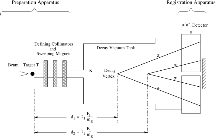
Figure 1: Simplified diagram of the typical neutral $K$-meson decay experiment.

The forward-light-cone condition (4.7a), (4.7b) expresses the intuitive notion of causality, that a state must be prepared first before an observable can be measured in it and that the probability for the observable in a prepared state cannot propagate faster than with the velocity of light. This intuitively evident, causality condition is here obtained as a consequence of the new hypothesis (1.9_∓) and is not fulfilled by unitary group representations in Hilbert space. To go into more detail, we shall use for our discussions of the correspondence between theory and experiment the decay of the neutral Kaons (as occurs e.g. in the reaction $\pi^{-}p\rightarrow\Lambda K^{\circ}$, $K_{S}^{\circ}\rightarrow\pi^{+}\pi^{-}$, cf. also Figure $1$ of [2]) for which there exists a series of famous experiments [17, 18]. A simplified schematic diagram of these experiments is given in Figure 1.

A $K^{\circ}$ is produced with a time scale of $10^{-23}$ s by strong interaction and it decays by weak interaction with a time scale of $10^{-10}$ s, which is roughly the lifetime of the $K_{S}^{\circ}$, $\tau_{K_{s}}$. This defines very accurately the time $t_{0}$ at which the preparation of the $K^{\circ}$-state is completed and the registration of the decay products can begin (theoretical uncertainty is $10^{-13}\tau_{K}$). The $K^{\circ}$-state is created instantly at the baryon target $T$ (the baryon $p$ is excited from the ground state (proton) into the $\Lambda$ state, with which we are no further concerned), and a beam of $K^{\circ}$ emerges from $T$. We imagine that single Kaons, created at a collection of initial times $t_{0}^{(n)}$, are moving into the forward direction $\boldsymbol{x}=(0,0,z)$. Each $t_{0}^{(n)}$ at which the $n$-th Kaon is created is identified with the same mathematical semigroup time $t_{0}=0$ of the transformation formula (3), (3.6), etc.

One selects $K^{\circ}$’s that have a fairly well defined momentum, and we want to discuss first the case that it is described by a Gamow vector $|\boldsymbol{\hat{p}}j_{3}[\mathsf{s}_{R}j_{R}]^{-}\rangle$ with $\mathsf{s}_{R}=(M_{S}-i\Gamma_{S}/2)^{2},\ \frac{\Gamma_{S}}{M_{S}}=10^{-14}$, and with a well defined 4-velocity $\boldsymbol{\hat{p}}$, i.e., with a momentum $\boldsymbol{p}=\sqrt{\mathsf{s}_{R}}\boldsymbol{\hat{p}}\approx M_{S}\boldsymbol{\hat{p}}$. Whether such idealized states exist is the analogue of the question whether plane-wave states of stable particles $|\boldsymbol{p}[mj]\rangle$ exist; certainly it cannot be tested experimentally because any macroscopic apparatus can measure the particle momentum $\boldsymbol{p}=m\boldsymbol{\hat{p}}$ only within a certain momentum interval around $\boldsymbol{p}$. But we are used to working with Dirac kets and thinking of them as states with precise momentum $\boldsymbol{p}$ (or 4-velocity $\boldsymbol{\hat{p}}$). Below in (4) we will discuss continuous superpositions with sharply peaked 4-velocity $\boldsymbol{\hat{p}}_{0}$.

We consider first the idealized Kaon state described by the Gamow ket $|\boldsymbol{\hat{p}}[\mathsf{s}_{S}]^{-}\rangle$ with $\sqrt{\mathsf{s}_{S}}={M_{S}-i\Gamma_{S}/2}$. Since $\Gamma_{S}\ll M_{S}$, $\Gamma_{S}$ can be safely neglected when the velocity $\boldsymbol{\hat{p}}$ is experimentally determined as $\boldsymbol{\hat{p}}=\boldsymbol{p}/M_{S}$ $=$ $({\boldsymbol{{p}}}_{\pi^{+}}+{\boldsymbol{{p}}}_{\pi^{-}})/M_{S}$.

Somewhere downstream in Figure 1 at a distance $z=d_{1},d_{2},\cdots,d_{n},\cdots$ from $T$, we “see” a decay vertex for $\pi^{+}\pi^{-}$. A detector (registration apparatus) has been built such that it counts $\pi^{+}\pi^{-}$ pairs which are coming from the position $\boldsymbol{x}=(0,0,z)$. The observable registered by the detector is the projection operator

$$\Lambda(x)=|\psi^{-}(t,\boldsymbol{x})\rangle\langle\psi^{-}(t,\boldsymbol{x})|=|\pi^{-}\pi^{+},t\rangle\langle\pi^{+}\pi^{-},t|$$ (4.9)

for those $\pi^{-}\pi^{+}$ which originate from the fairly well specified location $x=(t,\boldsymbol{x})=(t,0,0,z)$.

More realistically $\Lambda$ should be a projection operator on a multidimensional subspace of $\Phi_{+}$ describing the decay products $\pi^{+}\pi^{-}$ counted by the detector (with finite energy and angle resolution) of which we consider here the one dimensional subspace described by the pure out-state vector $\psi^{-}=|(\pi^{+}\pi^{-})\rangle\in\Phi_{+}$, (4.9). This means that its energy wave function $\langle^{-}\mathsf{s}|\psi^{-}\rangle$ is a smooth Hardy function $\langle\mathsf{s}^{-}|\psi^{-}\rangle\in{\cal H}^{2}_{+}$ which can be analytically continued into the complex $\mathsf{s}$-plane.

Before we consider the experiment of Figure 1, let us discuss the situation that the ($\pi^{+}\pi^{-}$)-detector represented by $|\psi^{-}\rangle\langle\psi^{-}|$ is in the rest frame of the decaying $K^{\circ}$. In its rest frame, the decaying $K^{\circ}$ evolves in time according to $e^{-iH^{\times}\tau}|0,\mathsf{s}_{S}^{-}\rangle=e^{-i\sqrt{\mathsf{s}_{S}}\tau}|0,\mathsf{s}_{S}^{-}\rangle$, where $\tau$ is the proper time (in the $K^{\circ}$ rest frame) and $\sqrt{\mathsf{s}_{S}}=(M_{S}-i\Gamma_{S}/2)$. Thus, the probability rate density for counting the $\pi^{+}\pi^{-}$ by the detector in the $K^{\circ}$ rest frame is according to (4.3) and (4.6) proportional to

$$|\langle\psi^{-}|e^{-iH^{\times}\tau}|0,\mathsf{s}_{S}^{-}\rangle|^{2}=|\langle e^{iH\tau}\psi^{-}|0,\mathsf{s}_{S}^{-}\rangle|^{2}=e^{-\Gamma_{S}\tau}|\langle\psi^{-}|0,\mathsf{s}_{S}^{-}\rangle|^{2}$$ (4.10)

This is the usual exponential dependence upon the time $\tau$ in the rest frame.

In practice [17, 18], one does not measure the counting rate by detectors in the rest system of the $K^{\circ}$, but one has a $K^{\circ}$ that moves with a fairly well defined momentum $\boldsymbol{p}$ into the $z$-direction (beam direction, cf. Figure 1). One measures the counting rate as a function of the distance $z$ from the position $T$ at which the $K^{\circ}$’s have been produced. The formula for this distance dependence of the counting rate is usually justified from relativistic kinematics of classical particles. Here we want to derive this formula by relativistic quantum theory from the transformation property (3.6) of the Poincaré semigroup and therewith obtain experimental support of the theoretical result (3.6) derived from the hypothesis (1.9_∓).

In the experiment depicted schematically in Figure 1, one has instead of the detector $|\psi^{-}\rangle\langle\psi^{-}|$ and a decaying $K^{\circ}$-state $|0,\mathsf{s}_{S}^{-}\rangle$ at rest a decaying $K^{\circ}$-state $|\boldsymbol{\hat{p}},\mathsf{s}_{S}^{-}\rangle$ with momentum $\boldsymbol{{p}}\approx M_{S}{\boldsymbol{\hat{p}}}$ and the detectors $|\psi(x)^{-}\rangle\langle\psi^{-}(x)|$ scan the whole flight path of the Kaon along the $z$-axis, $\boldsymbol{x}=(0,0,z)$ (in the lab frame).

The detector that counts the decay event $K^{\circ}\rightarrow\pi^{-}\pi^{+}$ at $\boldsymbol{x}$ is obtained from the detector $|\psi^{-}\rangle\langle\psi^{-}|$ at a reference position $x_{1}=(t_{1},\boldsymbol{x}_{1})$ (e.g., counting the decay events $K^{\circ}\rightarrow\pi^{-}\pi^{+}$ at time $t_{1}=t_{0}=0$ directly at the target position $\boldsymbol{x}_{1}=\boldsymbol{x}_{T}=0$) by a space-time translation $U(I,x)=U(I,(t,\boldsymbol{x}))$:

$$|\psi(x)^{-}\rangle=U(I,(t,\boldsymbol{x}))|\psi^{-}\rangle,\ x^{2}\geq 0,\ t\geq 0$$ (4.11)

In order that this space-time position $(t,\boldsymbol{x})$ of the detector runs with the $K^{\circ}$ that is moving with velocity $\boldsymbol{\hat{p}}\approx\boldsymbol{p}/M_{S}$ along the $z$=axis, the parameters $(t,\boldsymbol{x})$ (of the space-time translation of the classical apparatus) must fulfill $\frac{\boldsymbol{x}}{t}=\frac{\boldsymbol{\hat{p}}}{\gamma}=\boldsymbol{v}$, since $\boldsymbol{v}$ is the velocity in the lab frame of the particle $K^{\circ}$. The parameters of the space-time translation $(t,\boldsymbol{x})$ from position $(t_{0}=0,{\boldsymbol{x}}_{T}=0)$ at which the decaying particle has been created to position $(t,0,0,z)$ at which the decay event is counted (i.e., the distance from $T$ to the decay vertex in Figure 1) is thus given by

$$x=(t,\boldsymbol{x})=(t,0,0,z=tv)=(\frac{z}{v},0,0,z)=(\gamma\tau,0,0,\tau\hat{p})$$ (4.12)

To obtain the prediction for the measured counting rate we have thus to calculate the probability density amplitude $\langle\psi^{-}(x)|{\boldsymbol{\hat{p}}},\mathsf{s}_{S}^{-}\rangle$ and the probability rate for a decay event $\pi^{+}\pi^{-}$ at $x$ which is proportional to $|\langle\psi^{-}(x)|\boldsymbol{\hat{p}},\mathsf{s}_{S}^{-}\rangle|^{2}$. Using the transformation formula for the Gamow kets (3.6) in the probability amplitude

$$\langle\psi^{-}(x)|{\boldsymbol{\hat{p}}},\mathsf{s}_{S}^{-}\rangle=\langle U(I,x)\psi^{-}(x)|{\boldsymbol{\hat{p}}},\mathsf{s}_{S}^{-}\rangle=\langle\psi^{-}|U^{\times}(I,x)|\boldsymbol{\hat{p}},\mathsf{s}_{S}^{-}\rangle,\ t\geq 0,\ t\geq\boldsymbol{x}.\boldsymbol{v}$$ (4.13a)

we obtain from (4.3)

$$\langle\psi^{-}(t=\frac{z}{v},0,0,z)|{\boldsymbol{\hat{p}}},\mathsf{s}_{S}^{-}\rangle = e^{-i\gamma\sqrt{\mathsf{s}_{S}}(\frac{z}{v}-zv)}\langle\psi^{-}|{\boldsymbol{\hat{p}}},\mathsf{s}_{S}^{-}\rangle$$ (4.13)

$$= e^{-i(M_{S}-i\Gamma_{S}/2)\frac{z}{\gamma v}}\langle\psi^{-}|{\boldsymbol{\hat{p}}},\mathsf{s}_{S}^{-}\rangle$$

$$\text{for}\ t\geq 0,\ 1\geq v$$

Therewith we predict that the probability rate as a function of the distance $z$ from the target is proportional to

$$|\langle\psi^{-}(x)|{\boldsymbol{\hat{p}}},\mathsf{s}_{S}^{-}\rangle|^{2}=e^{-\Gamma_{S}\frac{z}{\gamma v}}|\langle\psi^{-}|{\boldsymbol{\hat{p}}},\mathsf{s}_{S}^{-}\rangle|^{2}=e^{-\frac{z}{\gamma\beta c}\Gamma_{S}}|\langle\psi^{-}|{\boldsymbol{\hat{p}}},\mathsf{s}_{S}^{-}\rangle|^{2},\quad t\geq 0,\ 1\geq v/c$$ (4.14)

where we have reverted to the standard units with light speed $c$ and $\beta=\frac{v}{c},\ \gamma=\frac{1}{\sqrt{1-(v/c)^{2}}},\ v=\frac{\hat{p}}{\gamma}=\frac{p}{\gamma(M_{S}-i\Gamma/2)}\approx\frac{p_{z}}{\gamma M_{S}}$. The momentum $p_{z}$ is measured as the $z$-component of the $\pi^{+}\pi^{-}$-system, $p_{z}=(p_{\pi^{+}}+p_{\pi^{-}})_{z}$. With (4.12), the exponential in (4.14) is

$$e^{-\Gamma_{S}\frac{z}{\gamma v}}=e^{-\Gamma_{S}t/\gamma}=e^{-\Gamma_{S}\tau},\quad\tau\geq 0$$ (4.14a)

The result (4.14) is identical to the formula used for fitting the $\pi^{+}\pi^{-}$ counting rate, e.g., equation (23), (24) of [18] for $K^{\circ}$ and (1) of [19] for the $B^{\circ}$. It has the advantage of fitting the rate as a function of distance making use of time dilation. But even more important is the fact that (4.14) does not require the knowledge of the creation times $t_{0}^{(n)}$ for each individual member of the ensemble of $K^{\circ}$’s.

We thus have the following situation: An ensemble of $K^{\circ}$’s is created at various times $t_{0}^{(n)}$ in the laboratory (over months etc of the run of the experiment) at the position $T$ with $z=0$. The $n$-th $K^{\circ}$ moves down the beam line during the time interval $t_{n}-t_{0}^{(n)}$ and decays at $t_{n}$ after it has moved the distance $z=v(t_{n}-t_{0}^{(n)})=\frac{p_{z}}{\gamma M_{S}}(t_{n}-t_{0}^{(n)})=v\gamma\tau_{n}=\frac{p_{z}}{M_{S}}\tau_{n}$. The ensemble of $K_{S}^{\circ}$ created at these different times $t^{(n)}_{0}$, which are all represented by the same semigroup time $t_{0}=0$, is described by the (almost) momentum eigenvector $\phi^{G}_{\mathsf{s}_{S}}(t)=U^{\times}(I,(t,0,0,t\boldsymbol{v}))|\boldsymbol{\hat{p}}\mathsf{s}_{S}^{-}\rangle$ (or by $\phi^{G}_{p_{0}\mathsf{s}_{R}}$ below). This generalized state vector is evolving in spacetime (starting at $(t_{0}=0,\ \boldsymbol{x}_{T}=0$) and as a consequence the probability rate for the $\pi^{+}\pi^{-}$ at $(t,0,0,z)$ changes according to (4.14). It is this probability rate as a function of $z=\frac{p}{\gamma M_{S}}(t-0)$ which is measured by the counting rate $\frac{\Delta N(t)}{\Delta t}$ (number of decay events $\Delta N(t)$ per time interval $\Delta t$) at the discrete set of points $d_{n}=\frac{p}{\gamma M_{S}}(t_{n}-t_{0}^{(n)})=\frac{p}{\gamma M_{S}}(t-0)=z$, which is then fitted to (4.14) in order to determine the value of $\Gamma_{S}$ which according to (4.14a) is the inverse lifetime, $\Gamma_{S}=\frac{\hbar}{\tau_{S}}$.

Thus the Kaon-state vector $\phi^{G}_{\mathsf{s}_{S}}(t),t\geq 0$ describes an ensemble of individual $K^{\circ}_{S}$ (with the same momentum $p$) which are created at quite different times $t_{0}^{(n)}$. All these times $t_{0}^{(n)}$ in the past of the individual $K_{S}^{\circ}\rightarrow\pi^{+}\pi^{-}$ events are the initial time $t_{0}=0$ for the $K^{\circ}$-state $\phi_{\mathsf{s}_{S}}^{G}(t)$. This time $t_{0}$ at which $\phi^{G}_{\mathsf{s}_{S}}$ has been created and after which one can count the decay products, i.e., the time $t=0$ in the “life” of each individual $K^{\circ}$, is identified with the mathematical semigroup time $t=0$. The vector $\phi^{G}$ does not represent a bunch (wave packet) of $K^{\circ}$’s moving down the beam line together. But it represents an ensemble of $K^{\circ}$’s which are created at quite arbitrary times $t_{0}^{(n)}$ under the same conditions. They have a well defined lifetime $\tau={\rm average\ of}\ \frac{1}{\gamma}(t_{n}-t^{(n)}_{0})$.

In the past, (4.14) has been justified by applying relativistic kinematics to the $K^{\circ}_{S}$ and treating it as a classical particle. Here we have derived it from the transformation property of the projection operator $|\psi^{-}\rangle\langle\psi^{-}|$ which represents the registration apparatus of the decay products. The prediction (4.14) also contains the time asymmetry $t_{n}-t_{0}^{(n)}=t>0$, which is also always tacitly assumed because it is an obvious consequence of our feeling for causality (the decay products can only be counted after the preparation of each $n$-th $K^{\circ}$ at the position ${\boldsymbol{x}}_{T}$ at $t_{0}^{(n)}$). Here it is also a consequence of (3.6).

Since we use the relativistic Gamow vectors $|{\boldsymbol{\hat{p}}},\mathsf{s}_{S}^{-}\rangle$ defined from the position of an $S$-matrix pole at $\mathsf{s}_{S}=(M_{S}-i\Gamma_{S}/2)^{2}$, we also derive (by (4.13) and (4.14)) that the inverse of $\Gamma_{S}$ is exactly the lifetime $\tau_{S}$ in the rest frame, $\tau_{S}=\frac{\hbar}{\Gamma_{S}}$. This is also often tacitly assumed but has previously only been justified by the Weisskopf-Wigner approximation in the non-relativistic case [21]. This result, which one can only obtain for the relativistic Gamow vector with Breit-Wigner energy distribution (1.17), is the reason for which we prefer the parameterization $\sqrt{\mathsf{s}_{R}}=(M_{R}-i\Gamma_{R}/2)$, or, the definition $\Gamma_{R}=-2{\rm Im}\sqrt{\mathsf{s}_{R}}$ over other definitions, (5.37) of [2], for the width of the lineshape of a relativistic resonance [26, 27].

We shall now relax the assumption of an exact 4-velocity eigenstate $|{\boldsymbol{\hat{p}}},\mathsf{s}_{S}^{-}\rangle$ for the $K^{\circ}$ and start from the assumption that $K^{\circ}$ is represented by a resonance state which has a realistic (not $\delta^{3}(\boldsymbol{\hat{p}}-\boldsymbol{\hat{p}}_{0})$) 4-velocity distribution $\phi_{j_{3}}(\hat{p})$ which however is strongly peaked at the value $\boldsymbol{\hat{p}}_{0}$. This will lead to results which can be directly connected to formulas previously given by some heuristic arguments which also made use of 4-velocity eigenvectors for unstable relativistic particles [16].

From (3.6) it follows that the space-time translation of a momentum wave-packet (1.22) peaked at $\boldsymbol{p}_{0}$ is given by

$$U^{\times}(I,x)\phi^{G}_{\boldsymbol{p}_{0}\mathsf{s}_{R}}=\sum_{j_{3}}\int\frac{d^{3}\boldsymbol{\hat{p}}}{2\hat{p}^{0}}e^{-i\gamma\sqrt{\mathsf{s}_{R}}(t-\boldsymbol{x}.\boldsymbol{v})}|\boldsymbol{\hat{p}}j_{3}[\mathsf{s}_{R}j_{R}]^{-}\rangle\phi_{j_{3}}(\boldsymbol{\hat{p}})$$

$$\text{only for }t\geq 0,\ t\geq\boldsymbol{x}.\boldsymbol{v}$$ (4.15)

This represents the Gamow vector with a 4-velocity distribution described by the wave function $\phi_{j_{3}}(\boldsymbol{\hat{p}})=\phi_{j_{3}}(\gamma{\boldsymbol{v}})$ which has been time and space translated by the 4-vector $(t,\boldsymbol{x})$. Therefore the decay probability amplitude for this Gamow state $\phi^{\rm G}_{p_{0}\mathsf{s}_{R}}$ is (with $j=0$ for simplicity):

$$\langle\psi^{-}(x)|\phi^{\rm G}_{p_{0}\mathsf{s}_{R}}\rangle = \langle\psi^{-}|U^{\times}(I,x)|\phi^{\rm G}_{\boldsymbol{p}_{0}\mathsf{s}_{R}}\rangle$$ (4.16)

$$= \int\frac{d^{3}{\boldsymbol{\hat{p}}}}{2\hat{p}^{0}}e^{-i\sqrt{\mathsf{s}_{R}}\gamma(t-{\boldsymbol{x}}{\boldsymbol{v}})}\langle\psi^{-}|{\boldsymbol{\hat{p}}},\mathsf{s}_{R}^{-}\rangle\phi({\boldsymbol{\hat{p}}})$$

Here $t$ and $\boldsymbol{x}$ are the time and position at which the detector counts the decay events $\pi^{+}\pi^{-}$, and ${\boldsymbol{\hat{p}}}=\frac{\boldsymbol{p}}{\sqrt{\mathsf{s}_{R}}}$, $\boldsymbol{v}$ and $\gamma=\hat{p}^{0}$ refer to the prepared state of the $K^{0}$.

With the assumption that $\phi_{j_{3}}(\boldsymbol{\hat{p}})$ is strongly peaked about $\boldsymbol{\hat{p}_{0}}=\frac{\boldsymbol{v_{0}}}{\sqrt{1-\boldsymbol{v_{0}}^{2}}}=\gamma_{0}{\boldsymbol{v_{0}}}$, we can approximate the exponent in (4)

$$-i\gamma\sqrt{\mathsf{s}_{R}}(t-\boldsymbol{x}.\boldsymbol{v})=-i\sqrt{\mathsf{s}_{R}}\left(\sqrt{1+\boldsymbol{\hat{p}}^{2}}t-\boldsymbol{x}.\boldsymbol{\hat{p}}\right)$$

by expanding it around $\boldsymbol{\hat{p}_{0}}$ and retaining only the first order terms in $\boldsymbol{\hat{p}}-\boldsymbol{\hat{p}_{0}}$. Using the first order Taylor expansion of $\sqrt{1+\boldsymbol{\hat{p}}^{2}}$

$$\sqrt{1+\boldsymbol{\hat{p}}^{2}}\approx\sqrt{1+\boldsymbol{\hat{p}_{0}}^{2}}+\frac{\boldsymbol{\hat{p}_{0}}.(\boldsymbol{\hat{p}}-\boldsymbol{\hat{p}_{0}})}{\sqrt{1+\boldsymbol{\hat{p}_{0}}^{2}}}\,,$$ (4.17)

in (4), we obtain the approximate expression

$$\langle\psi(x)^{-}|\phi^{G}_{\boldsymbol{p}_{0}\mathsf{s}_{R}}\rangle\approx e^{-i{\sqrt{\mathsf{s}_{R}}}t/\gamma_{0}}\int\frac{d^{3}\hat{p}}{2\hat{p}^{0}}e^{i{\sqrt{\mathsf{s}_{R}}}{\boldsymbol{\hat{p}}}({\boldsymbol{x}}-{\boldsymbol{v_{0}}}t)}\langle\psi^{-}|{\boldsymbol{\hat{p}}},\mathsf{s}_{R}^{-}\rangle\phi(\boldsymbol{\hat{p}})$$ (4.18)

where we use $\boldsymbol{v_{0}}=\frac{\boldsymbol{\hat{p}_{0}}}{\gamma_{0}},\ \gamma_{0}=\sqrt{1+{\boldsymbol{\hat{p}}_{0}}^{2}}$.

For easier interpretation this is written as

$$\langle\psi^{-}(x)|\phi^{\rm G}_{\boldsymbol{p}_{0}\mathsf{s}_{R}}\rangle\approx e^{-i\sqrt{\mathsf{s}_{R}}\frac{t}{\gamma_{0}}}e^{i\sqrt{\mathsf{s}_{R}}({\boldsymbol{x}}-{\boldsymbol{v_{0}}}t){\boldsymbol{\hat{p}_{0}}}}A({\boldsymbol{x}}-{\boldsymbol{v_{0}}}t),\quad t\geq 0,\ t\geq\boldsymbol{x}.\boldsymbol{v}_{0}$$ (4.19)

where, following [16], $A({\boldsymbol{x}}-{\boldsymbol{v_{0}}}t)$ is defined as

$$A(\boldsymbol{x}-\boldsymbol{v_{0}}t)=\int\frac{d^{3}\hat{p}}{2\hat{p}^{0}}e^{i\sqrt{\mathsf{s}_{R}}(\boldsymbol{\hat{p}}-\boldsymbol{\hat{p}_{0}})(\boldsymbol{x}-\boldsymbol{v_{0}}t)}\langle\psi^{-}|{\boldsymbol{\hat{p}}},\mathsf{s}_{R}^{-}\rangle\phi(\boldsymbol{\hat{p}})$$ (4.20)

The reason for defining $A$ in this way is that for a sharp 4-velocity distribution of just one value $\boldsymbol{\hat{p}}_{0}=\gamma_{0}\boldsymbol{v_{0}}$ defined by

$$\phi(\boldsymbol{\hat{p}})=2{\hat{p}}^{0}\delta(\boldsymbol{\hat{p}}-\boldsymbol{\hat{p}_{0}})$$ (4.21)

one obtains for (4.20)

$$A(\boldsymbol{x}-{\boldsymbol{v_{0}}}t)=\langle\psi^{-}|\boldsymbol{\hat{p}_{0}}\mathsf{s}_{R}^{-}\rangle$$ (4.22)

Inserting this into (4.19), the probability density amplitude for this Gamow state $\phi_{p_{0}\mathsf{s}_{R}}^{G}$ in the limit of sharp 4-velocity $\boldsymbol{\hat{p}}_{0}$ is

$$\langle\psi^{-}(x)|\phi^{\rm G}_{\boldsymbol{\hat{p}}_{0}\mathsf{s}_{R}}\rangle\approx e^{-i\sqrt{\mathsf{s}_{R}}\gamma_{0}(t-{\boldsymbol{x}}.{\boldsymbol{v_{0}}})}\langle\psi^{-}|\boldsymbol{\hat{p}}_{0}\mathsf{s}_{R}^{-}\rangle,\quad t\geq 0,\quad t\geq\boldsymbol{x}.\boldsymbol{v}$$ (4.23)

Here we have not put any condition on the position $\boldsymbol{x}$ around which the $\pi^{+}\pi^{-}$ events are counted. If we now set the detector such that $\pi^{+}\pi^{-}$ events are counted at the position downstream at ${\boldsymbol{x}}={\boldsymbol{v_{0}}}t=(0,0,z)$, then we obtain from (4.23),

$$\langle\psi^{-}(t=\frac{z}{v_{0}},0,0,z)|\phi^{\rm G}_{\boldsymbol{p}_{0}\mathsf{s}_{R}}\rangle\approx e^{-i(M_{R}-i\Gamma_{R}/2)\frac{z}{v_{0}\gamma_{0}}}A(\boldsymbol{x}-\boldsymbol{v}_{0}t)\quad t\geq 0$$ (4.24)

so that the counting rate is predicted again to be proportional to

$$|\langle\psi^{-}(t=\frac{z}{v_{0}},0,0,z)|\phi^{\rm G}_{\boldsymbol{p}_{0}\mathsf{s}_{R}}\rangle|^{2}\approx e^{-\Gamma_{R}\frac{z}{v_{0}\gamma_{0}}}A(\boldsymbol{x}-\boldsymbol{v}_{0}t)\quad t\geq 0$$ (4.25)

which agrees with (4.14) for $\boldsymbol{\hat{p}}_{0}=\boldsymbol{\hat{p}}$ as it should for the sharp velocity distribution (4.21). $A(\boldsymbol{x}-\boldsymbol{v_{0}}t)$ thus describes the deviation of the $K^{\circ}$ beam from a sharp momentum beam.

The expressions (4.19) and (4.20) –which agree with [16] except that here causality (4.7) is also a result– represents a wave packet traveling with velocity $\boldsymbol{v_{0}}$ and simultaneously decaying exponentially with a lifetime $\tau_{R}=1/\Gamma_{R}$. Thus the probability amplitude for the decay events $K^{\circ}\rightarrow\pi^{+}\pi^{-}$ is a wave packet that travels with velocity ${\boldsymbol{v_{0}}}={\boldsymbol{\hat{p}_{0}}}(1+{\boldsymbol{\hat{p}_{0}}})^{-1/2}$, where $\boldsymbol{\hat{p}_{0}}$ is the central value of the sharply peaked 4-velocity distribution in the prepared $K^{\circ}$-state, and decays in time. This, however, does not mean that a wave packet of $K^{\circ}$-mesons is traveling down the $z$-direction because the time $t$ is the time interval from the creation of the $n$-th $K^{\circ}$ at the time $t_{0}^{(n)}$ and this time $t_{0}^{(n)}$ is a different time by the clocks in the lab for each single $K^{\circ}$ decay event. The state $|\phi^{\rm G}_{\mathsf{s}_{R}}\rangle\langle\phi^{\rm G}_{\mathsf{s}_{R}}|$ describes an ensemble of single microphysical decaying systems $K^{\circ}$ each of which has been produced by the macroscopic preparation apparatus and a quantum scattering process at different times $t_{0}^{(n)}$ in the lab. All of these $t_{0}^{(n)}$ are mathematically represented by the semigroup time $t=0$ which represents the creation time in the life of each $K^{\circ}$. Each event (labeled by $n$) counted by the detector at the position $z=d_{n}=v_{0}(t_{n}-t_{0}^{(n)})$ is the result of the decay of such a single microsystem that was created at $t_{0}^{(n)}$ and traveled the distance $d_{n}$ (the different $t_{0}^{(n)}$ can be days apart).

For a detector counting the events at $d_{n}$, the ensemble of decaying $K^{\circ}$-mesons is not a wave packet traveling in the $z$-direction but it is an ensemble of individual decay events of Kaons which were created at the times $t_{0}^{(n)}$. And each individual time $t_{0}^{(n)}$ is equal to the semigroup time $t=0$ of the causal Poincaré transformations (3.6) and (2.17_-).

To conclude this section, we wish to emphasize that neither the momentum wave-packets (1.22) of (4) nor the eigenkets $|\boldsymbol{\hat{p}}[\mathsf{s}_{R}]^{-}\rangle$ of (3.6) represent precisely the apparatus prepared Kaon state vector (besides the fact that a realistic prepared $K^{\circ}$ state is not a pure state but a mixture). The in-state vector $\phi^{+}_{K^{\circ}}\in\Phi_{-}$ of the $K^{\circ}$-beam, prepared by the accelerator and by scattering on the baryon target $T$, is given by the complex basis vectors expansion (1.21), (1.24). For the case of a double resonance system, such as the $K_{S}$–$K_{L}$ system with resonance poles at $\mathsf{s}_{L/S}=(M_{L/S}-i\Gamma_{L/S}/2)^{2}$ in the $j_{R}=0$ partial wave, it is given according to (1.24) and (1.22) by

$$\phi^{+}_{\boldsymbol{p}_{0}K^{\circ}} = \int\frac{d^{3}\hat{p}}{2\hat{p}^{0}}(|\boldsymbol{\hat{p}}j_{3}[\mathsf{s}_{S}j_{R}]^{-}\rangle+|\boldsymbol{\hat{p}}j_{3}[\mathsf{s}_{L}j_{R}]^{-}\rangle)\phi(\boldsymbol{\hat{p}})+|{B}\rangle$$

$$= \phi^{G}_{\mathsf{s}_{S}}+\phi^{G}_{\mathsf{s}_{L}}+|B\rangle$$

where $\phi^{G}_{\mathsf{s}_{S,L}}$ is the Gamow vector of $K^{\circ}_{S,L}$ that evolves exponentially by the exact Hamiltonian $H=H_{0}+H_{W}$ and $|B\rangle$ is the background vector representing the non-resonant background in the $K^{\circ}$-production. The state vectors $\phi^{G}_{\mathsf{s}_{S,L}}$ describe the exponential decay and $|B\rangle$ is an integral over the energy-continuum [20]. The 4-velocity wave function $\phi(\boldsymbol{\hat{p}})$ is peaked at a value $\hat{p}_{0}\approx\frac{p_{0}}{M_{S}}\approx\frac{p_{0}}{M_{L}}$

In the Weisskopf-Wigner approximation [21], which amounts to the omission of the background integral $|B\rangle$, (4) reduces to the superposition of $K_{S}$- and $K_{L}$-Gamow vector:

$$\phi^{+}_{K^{\circ}}\approx\phi^{S}_{\mathsf{s}_{S}}+\phi^{L}_{\mathsf{s}_{L}}$$ (4.27)

This is the approximation that is always used for the $K^{\circ}$-system and $B^{0}$-system following [22]. We apply now the transformation $U^{\times}(I,x)$ with $x$ given by (4.12) to (4.27) as done in (4.25) etc., and obtain in place (4.24) for the probability density amplitude of the state (4.27):

$$\psi^{-}(t=\frac{z}{v_{0}},0,0,z)|\phi^{+}_{K^{\circ}}\rangle \approx \left(e^{-i\frac{z}{v_{0}\gamma_{0}}(M_{S}-i\Gamma_{S}/2)}+e^{-i\frac{z}{v_{0}\gamma_{0}}(M_{L}-i\Gamma_{L}/2)}\right)A(\boldsymbol{x}-\boldsymbol{v_{0}}t)$$

$$\qquad\qquad\qquad\qquad\qquad t\geq 0$$

where $A$ is defined in (4.20). This is the standard expansion used in the $K^{\circ}$-experiments [17, 18]. It is the superposition of two exponentials. The time evolution of the background integral $|B\rangle$ in (4) is non-exponential and would lead to deviations from the exponential law (4). The time dependence of the background depends upon the preparation of the state $\phi^{+}$ and thus can vary substantially from experiment to experiment, whereas the time dependence of the Gamow state $\phi^{G}_{j_{R}\mathsf{s}_{R_{n}}}$ is always exponential with the same inverse lifetime $\frac{1}{\tau_{R_{i}}}=\Gamma_{R_{i}}$. The lifetimes $\tau_{R_{i}}$ are characteristic of the Gamow states (the resonances per se) and do not vary with the preparation of the in-state $\phi^{+}$.

The prediction (4) without the background term $|B\rangle$ reduces in the rest frame $\boldsymbol{\hat{p}}=\boldsymbol{0}$ to the time evolution obtained in the Lee-Oehme-Yang theory [22] which uses the heuristic assumption of a complex Hamiltonian. Here the time evolution is derived from the transformation property of relativistic Gamow vectors which describe $K_{S}$ and $K_{L}$ as decaying states defined by the $S$-matrix poles at $\mathsf{s}_{S,L}$ (resonances). Thus, the Lee-Oehme-Yang theory, which is based on the Wigner-Weisskopf approximation [21], is recovered in (4) from the exact complex basis expansion (4) by neglecting the background term. The fact that the $|K_{S}\rangle$ and $|K_{L}\rangle$ states evolve without mixing between each other as derived in (4) and (4) for the Hardy space functionals $\phi^{S}_{\mathsf{s}_{S}}$ and $\phi^{L}_{\mathsf{s}_{L}}$, cannot be obtained if one uses non-exponential Hilbert space vectors for $|K_{S}\rangle$ and $|K_{L}\rangle$. In fact, in an exact Hilbert space theory for the Kaon system, an (unobserved) vacuum regeneration phenomenon between $|K_{S}\rangle$ and $|K_{L}\rangle$ is unavoidable [23].

Comparing (4) with (4.27), the question arises: under what conditions and to what extent can the background term be neglected and the quasistable states be isolated by the preparation process? Even though a theoretical answer is not available, the accuracy with which the exponential decay law and (4) has been observed in some cases ([24], [25], and in particular [18]) indicates that, at least for $\frac{\Gamma}{m}\approx 10^{-14}-10^{-8}$, the resonance state can be isolated from its background to a very high degree of accuracy.

The situation is quite different for $\frac{\Gamma}{m}\approx 10^{-2}-10^{-1}$ (hadron resonances but also the $Z$-boson) where $\Gamma$ is measured (not as the inverse lifetime but) as the width of the relativistic Breit-Wigner which according to (1.17) is the energy wave function of the Gamow vector $\phi^{G}_{\mathsf{s}_{R},j}$. It is well known empirically that in the fit of the $j$-th partial scattering amplitude to the cross section data one always needs, in addition to the Breit-Wigner representing the resonance per se, a background amplitude $B(\mathsf{s})$ corresponding (theoretically) to the background vector $|B\rangle$. Thus for larger values of $\frac{\Gamma}{m}$, $B(\mathsf{s})$ and thus $|B\rangle$ may not be negligible.

The initial decay rate $\frac{\Gamma}{\hbar}\equiv{\rm inverse\ lifetime}\equiv\frac{1}{\tau}$, as measured by a fit of the counting rate to (4.14) or (4.25), and the resonance width $\Gamma_{R}$ of the relativistic Breit-Wigner as it appears in (1.17), are conceptually and observationally different quantities. The width $\Gamma_{R}$ is measured by the Breit-Wigner line shape in the cross section and the inverse lifetime is measured by the decay rate as a function of time $t$ or distance $z$, as in (4.25) or (4). The theoretical connection between these two quantities is given by the Gamow vectors which according to (1.17) have a Breit-Wigner energy wave function and the transformation property (3.6) from which one predicts (4.14). This leads to $\frac{1}{\tau}=\frac{\Gamma_{R}}{\hbar}$. Without the Poincaré semigroup representations this relationship cannot be established, although it is well accepted in non-relativistic quantum mechanics. In the relativistic case one was never quite sure whether it makes sense to speak of a resonance per se that can be defined unambiguously as an entity separated from the background and other resonances. This ambiguity in the definition of resonance mass and width in the relativistic regime has recently been debated extensively in the literature [26]. The Poincaré semigroup representations $[j_{R},\mathsf{s}_{R}=m_{R}-i\Gamma_{R}/2]$ provide an unambiguous definition of a relativistic resonance and its width and mass [27]. The relativistic Gamow kets that span these semigroup representations have the additional attractive feature that they generalize Wigner’s definition of relativistic stable particles [28].

5 Summary and Conclusion

The purpose of the paper was to give a detailed derivation of the properties of vectors which describe relativistic decaying states and resonances. In contrast to non-relativistic quantum theory, where one considered quasistable particles as unique states characterized by two numbers $E_{R}$ and $\Gamma_{R}=\frac{\hbar}{\tau}$ which can appear either as a resonance described by a Breit-Wigner energy distribution or as a decaying particle with an exponential time evolution, relativistic resonances were considered as complicated objects. Most commonly, they were defined in perturbation theory by the propagator using the on-the-mass-shell renormalization scheme and had a mass $M$ and an energy dependent width $\Gamma(\mathsf{s})$, the definition of which depended upon the renormalization scheme [26]. The definition of a resonance by the pole of the relativistic $S$-matrix is less arbitrary and characterizes the resonance by a complex pole position $\mathsf{s}_{R}$, which however does not define the resonance width $\Gamma_{R}$ and resonance mass $M_{R}$ separately. In the Particle Data Table [29] the relativistic quasistable particles are classified by a mass $M_{R}$ and a width $\Gamma$ or by a mass and a lifetime $\tau$.

The known relativistic quasistable particles fall into two categories: those for which one can measure the width of their lineshape (given by a relativistic Breit-Wigner or others) (when $\frac{\Gamma}{M_{R}}\sim 10^{-1}-10^{-4}$) and those for which one can measure the lifetime from the (usually) exponential decay rate (when $\frac{1}{\tau M_{R}}\lesssim 10^{-8}$). The relativistic Breit-Wigner lineshape is easily obtained from the $S$-matrix (Laurent expansion). To obtain the exponential probability rate one postulates heuristic non-relativistic Gamow functions and $N$-dimensional complex Hamiltonian matrices for the self-adjoint Hamiltonian operator (e.g., $N=2$ for the neutral Kaon system [22]). The questions how this complex matrix is derived from the self-adjoint Hamiltonian $H=P_{0}$ of the Poincaré time translations or whether $\frac{\hbar}{\tau}=\Gamma_{R}$ are not addressed, except perhaps in analogy to the non-relativistic case for which one justifies the lifetime-width relation by the Weisskopf-Wigner approximation [21].

In this and the preceding paper [2] we have addressed this question of the nature of a relativistic quasistable particle by starting with the most universally accepted definition of a resonance by the second sheet pole at $\mathsf{s}=\mathsf{s}_{R}$ of the analytically continued partial $S$-matrix $S_{j_{R}}(\mathsf{s})$, where $\mathsf{s}$ is the square of the scattering energy, $\mathsf{s}=p_{\mu}p^{\mu}=(p_{1}+p_{2})^{2}=(p_{3}+p_{4})^{2}$. This definition by itself is insufficient to derive satisfactory results because the relativistic in- and out- Lippmann-Schwinger scattering states [10] are ill defined and are attributed contradictory properties. On the one hand they are to fulfill out-going and incoming boundary conditions expressed by the $\mp i0$ in the Lippmann-Schwinger equation and on the other hand they are to furnish a unitary representation of the Poincaré group [11]. To give the two kinds of Lippmann-Schwinger kets with their infinitesimally imaginary energy $|\mathsf{s}^{-}\rangle=|\mathsf{s}_{II}-i0^{-}\rangle$ and $\langle^{+}\mathsf{s}|=\langle^{+}\mathsf{s}_{II}-i0|$ (i.e., $|\mathsf{s}^{+}\rangle=|\mathsf{s}+i0^{+}\rangle$) a mathematical meaning –in the same way as one defines the ordinary Dirac kets as functionals over the Schwartz space– we postulated that the in-states $\phi^{+}$ and out-observables (often called out-“states”) $\psi^{-}$ are elements of two different Hardy spaces (1.9_-) and (1.9₊). This means the energy wave functions $\langle^{+}\mathsf{s}|\phi^{+}\rangle=\langle^{+}\boldsymbol{\hat{p}}j_{3}[\mathsf{s}j]|\phi^{+}\rangle$ and $\langle^{-}\mathsf{s}|\psi^{-}\rangle=\langle^{-}\boldsymbol{\hat{p}}j_{3}[\mathsf{s}j]|\psi^{-}\rangle$ are postulated to be smooth Hardy functions (1.10_-), (1.10₊) analytic in the lower and upper half-plane (second sheet of the $S$-matrix), respectively. ($\langle\psi^{-}|\mathsf{s}^{-}\rangle=\overline{\langle^{-}\mathsf{s}|\psi^{-}\rangle}$ is Hardy in the lower half plane). Because of the $\mp i\epsilon$, the Lippmann-Schwinger kets $|\boldsymbol{\hat{p}}j_{3}[\mathsf{s}j]^{\mp}\rangle$ do not span a unitary representation $[\mathsf{s}j]$ of the Poincaré group as usually assumed [11]. But if defined as functionals $|\boldsymbol{\hat{p}}j_{3}[\mathsf{s}j]^{\mp}\rangle\in\Phi^{\times}_{\pm}$ one can show that they span an irreducible representation $[\mathsf{s}\mp i0,j]$ of the Poincaré semigroup transformations ${\cal P}_{\pm}$ into the forward and backward light cone, respectively (2.17_-), (2.17₊).

The immediate consequence of this is causal propagation of probability. The $S$-matrix element $(\psi^{-},\phi^{+})=(\psi^{out},S\phi^{in})$ given by $(5.1)$ $(5.10)$ of [2] represents the probability amplitude to detect the out-observable $\psi^{-}$ of (1.8) in the prepared in-state $\phi^{+}$ of (1.7). The observable $\psi^{-}$ can by (2.16_-) only be predicted in the forward light cone relative to the prepared state $\phi^{+}$ in $(4.25)$ of [2]. This is discussed in Section 4, in particular for the resonance state described by the Gamow vector.

Within the mathematical setting provided by the hypothesis (1.9) the Gamow kets $|\boldsymbol{\hat{p}}j_{3}[\mathsf{s}_{R}j]^{-}\rangle$ can be defined as the vectors with an ideal Breit-Wigner energy wavefunction (1.17). They are continuous antilinear functionals on $\Phi_{+}$. Moreover, they are generalized eigenvectors of the momentum operators with complex eigenvalues (1.18). In particular, they have a complex mass $\sqrt{\mathsf{s}_{R}}$. These complex eigenvalues of the self-adjoint momentum operators are obtained in the same way as the ordinary eigenvalues of the Dirac kets, only that the Schwartz rigged Hilbert space has to be replaced by the pair of Hardy rigged Hilbert spaces (1.9). The Gamow kets have been shown in [2] to be associated with a resonance pole in the second sheet of the relativistic $S$-matrix at $\mathsf{s}_{R}=(M_{R}-i\Gamma_{R}/2)^{2}$. From their transformation property (3.6) follows that they span a semigroup representation space of the causal Poincaré transformations (2.11) characterized by $[\mathsf{s}_{R}j]$, with $j$ representing spin of the resonating partial wave and, $\mathsf{s}_{R}$, the complex pole position. In order to retain as much similarity as possible with Wigner’s unitary representations (2.19) of the Poincaré group for stable particles $[m^{2}j]$ and to maintain the meaning of the spin $j$ of a resonance, only semigroup representations with minimally complex momentum are considered, which means that the momentum is given by $\boldsymbol{p}=\sqrt{\mathsf{s}_{R}}\boldsymbol{\hat{p}}$, where the 4-velocities $\hat{p}^{0}=\gamma=\sqrt{1-\boldsymbol{v}^{2}},\ \boldsymbol{\hat{p}}=\gamma\boldsymbol{v}$ are real. The general transformation formula of the relativistic Gamow kets under causal Poincaré transformations ${\cal P}_{+}$ is given by (3.6) which looks very similar to Wigner’s unitary Poincaré group transformation, but differs by the property that transformations are allowed only into the forward light cone. From (3.6) follows the exponential time evolution (4.10) for an isolated Gamow state at rest and the exponential decay law (4.14) for a Gamow state moving with constant velocity $v=\beta c$ along the $z$-direction, as it has been used in experiments [18, 19].

The prepared state $\phi^{+}$ is in general not given by a Gamow vector but it is a linear superposition of Gamow vectors for all the $N$ resonance poles of the $j$-th partial $S$-matrix $S_{j}(\mathsf{s})$ and in addition there is a background vector (1.21), (1.24). Thus the prepared state is given by the complex basis vector expansion (4), which is very similar to the heuristic expansion in terms of eigenstates with complex eigenvalues $(M_{i}-\Gamma_{i}/2)$ for a finite dimensional effective Hamiltonian, like e.g., of the $K^{\circ}$-system in (4.27). Due to the background vector $|B\rangle$ over the energy continuum (which is always lost in the Weisskopf-Wigner approximation) one obtains in general also deviations from the exponential decay law for a prepared in-state $\phi^{+}$. This explains that in spite of the exponential time evolution for the Gamow state, describing the resonance per se, one may observe deviations from the exponential law even if there is only one resonance present.

The resonance per se is characterized by $(M_{R},\Gamma_{R})$ and has exponential evolution and according to (4.10) one predicts for the lifetime of a resonance with Breit-Wigner width $\Gamma_{R}$ that $\tau_{R}=1/\Gamma_{R}$. The validity of lifetime $=$ inverse width relation for $\Gamma_{R}$ and not for any of the other width definitions, e.g., $(5.37)$ of [2], removes the ambiguity in the definition of resonance mass and width [26] for relativistic resonances. It predicts that the width and mass is given by $M_{R}$, $\Gamma_{R}$ and that the lineshape of the resonance per se is given by the “exact” relativistic Breit-Wigner $(5.29)$ of [2]. This also fixes the background amplitude as the difference of the scattering amplitude and the “exact” Breit-Wigner $(5.25)$ of [2]. The parameters $(M_{R},\Gamma_{R}=\frac{1}{\tau_{R}})$ do not depend upon the experiment that prepares the state. For different experiments with different prepared in-states the background term in the amplitude and in the state vector (1.24), may change from experiment to experiment, and so will the deviation from the exponential decay law. But the parameters $(M_{R},\Gamma_{R})$ for the resonance per se and the lineshape of the resonance per se will not depend upon the experiment. Eliminating the background in the analysis of the decay data for each particular experiment should reveal the exponential character of decay.

Appendix A Mathematical Results

Here we prove that for any space-time translation by a $4$-vector $x$, such that $x^{2}\geq 0$, $t<0$, there exists $\psi^{-}\in\Phi_{+}$ such that $U(I,x)\psi^{-}\notin\Phi_{+}$. The proof contained in Proposition A.1 uses simple arguments based on the following results:

• Characterization of Hardy class functions on a half-plane
  The standard definition of ${\cal H}_{\pm}^{2}$ is the following [30]:

  Definition A.1 (${\cal H}_{\pm}^{p}$ $1\leq p<\infty$).

  A complex function $f(x+iy)$ analytic in the open lower half complex plane ${\mathbb{C}}_{-}$ is said to be a Hardy class function from below of order $p$, ${\cal H}_{-}^{p}$, if $f(x+iy)$ is $L^{p}$-integrable as a function of $x$ for all $y<0$ and

  $$\underset{y<0}{\rm sup}\int_{-\infty}^{\infty}dx\,\,|f(x+iy)|^{p}<\infty\,.$$ (A.1a)

  Similarly, a complex function $$f(x+iy) {\mathbb{C}}_{+} p {\cal H}_{+}^{p} f(x+iy) L^{p} x y>0$$ analytic in the open upper half complex plane is said to be a Hardy class function from above of order , , if is -integrable as a function of for all , and

  $$\underset{y>0}{\rm sup}\int_{-\infty}^{\infty}dx\,\,|f(x+iy)|^{p}<\infty\,.$$ (A.1b)

  In [14], it is shown that for $p=2$ (A.1a) is equivalent to

  $$\underset{-\pi<\phi<0}{\rm sup}\int_{0}^{\infty}|f(re^{i\phi})|^{2}dr<\infty\,,$$ (A.2a)

  and that (A.1b) is equivalent to

  $$\underset{0<\phi<\pi}{\rm sup}\int_{0}^{\infty}|f(re^{i\phi})|^{2}dr<\infty\,.$$ (A.2b)

  The definition of Hardy class functions given in (A.2a) and (A.2b) is the one that we shall use for proving our result. This is because the transformation $z\rightarrow\sqrt{z}$ converts a radial path of integration into another radial path, while it distorts the horizontal paths of integration in (A.1a) and (A.1b). Further, in the following we use the term Hardy (class) functions for functions obtained by taking the pointwise limit $y\rightarrow 0$ in (A.1) and (A.2).
  

• Characterization of $\tilde{\cal S}\cap{\cal H}_{\mp}^{2}$
  

  Definition A.2 ($\tilde{\cal S}$).

  The space $\tilde{\cal S}$ is defined as the space of Schwartz functions that vanish at zero faster than any polynomial, i.e., the space of $C^{\infty}$ functions for which

  $$\|f\|_{N}=\underset{\mathsf{s}\in{\mathbb{R}}}{\rm sup}\,\,\underset{n\leq N}{\rm sup}\left(|\mathsf{s}|+\frac{1}{|\mathsf{s}|}\right)^{N}\left|\frac{d^{n}f(\mathsf{s})}{d\mathsf{s}^{n}}\right|<\infty\,,\quad N=0,1,2,\cdots\,.$$

  Definition A.3 ($\widehat{M}({\mathbb{R}}_{\pm})$).

  The spaces $\widehat{M}({\mathbb{R}}_{\pm})$ are the spaces of Schwartz functions with supports in ${\mathbb{R}}_{+}=(0,\infty)$ and ${\mathbb{R}}_{-}=(-\infty,0)$ with vanishing moments of all orders, i.e.,

  $$\widehat{M}({\mathbb{R}}_{+})=\left\{f\in{\cal S}({\mathbb{R}})/\text{supp}f\subset(0,\infty)/\int_{0}^{\infty}x^{n}f(x)dx=0\,,\quad n=0,1,2,\cdots\right\}\,,$$

  $$\widehat{M}({\mathbb{R}}_{-})=\left\{f\in{\cal S}({\mathbb{R}})/\text{supp}f\subset(-\infty,0)/\int_{-\infty}^{0}x^{n}f(x)dx=0\,,\quad n=0,1,2,\cdots\right\}\,.$$

  Using the Payley-Wiener theorem, it can be shown that the Fourier transform is a continuous bijective functional from $\widehat{M}({\mathbb{R}}_{\pm})$ onto $\tilde{\cal S}\cap{\cal H}_{\mp}^{2}$:

  $${\cal F}:\,\,\widehat{M}({\mathbb{R}}_{\pm})\rightarrow\tilde{\cal S}\cap{\cal H}_{\mp}^{2}\,.$$ (A.3)

With these two results, our statement will follow from simple considerations.

Lemma A.1.

Left $f\in\tilde{\cal S}\cap{\cal H}_{-}^{2}$. Define $F_{\mp}(z)$ by

$$F_{-}(z)=\frac{f(\sqrt{z})}{z^{1/4}}$$

and

$$F_{+}(z)=\frac{f(-\sqrt{z})}{z^{1/4}}\,,$$

with the branch of $\sqrt{z}$ and $z^{1/4}$ taken as

$$-\pi\leq{\rm Arg}\,z<\pi\,.$$ (1.15)

Then $F_{\mp}\in\tilde{\cal S}\cap{\cal H}_{\mp}^{2}$.

Proof.

We note that, since the branch of $\sqrt{z}$ and $z^{1/4}$ is taken on the real axis, $F_{-}$ is analytic on ${\mathbb{C}}_{-}$ and $F_{+}$ is analytic on ${\mathbb{C}}_{+}$. The boundary values on the real axis of $F_{\pm}$ are given by

$$F_{-}(x)=\begin{cases}\frac{f(\sqrt{x})}{x^{1/4}}\,,&\quad x\geq 0\\ \frac{f(-i\sqrt{|x|})}{e^{-i\pi/4}|x|^{1/4}}\,,&\quad x\leq 0\,,\end{cases}$$ (A.4)

$$F_{+}(x)=\begin{cases}\frac{f(-\sqrt{x})}{x^{1/4}}\,,&\quad x\geq 0\\ \frac{f(-i\sqrt{|x|})}{e^{i\pi/4}|x|^{1/4}}\,,&\quad x\leq 0\,.\end{cases}$$ (A.5)

Since $f\in\tilde{\cal S}$, it follows from (A.4) and (A.5) that $F_{\pm}\in\tilde{\cal S}$. It remains to show that $F_{\pm}\in\tilde{\cal S}\cap{\cal H}_{-}^{2}$.

By performing the transformation $\phi\rightarrow\phi/2$ and $r\rightarrow\sqrt{r}$ in (A.2a), we obtain

$$\underset{-2\pi<\phi<0}{\rm sup}\int_{0}^{\infty}|f(\sqrt{r}e^{i\phi/2})|^{2}\frac{dr}{2\sqrt{r}}<\infty$$

Thus

$$\underset{-2\pi<\phi\leq-\pi}{\rm sup}\int_{0}^{\infty}|f(\sqrt{r}e^{i\phi/2})|^{2}\frac{dr}{\sqrt{r}}<\infty$$ (A.6)

$$\underset{-\pi\leq\phi<0}{\rm sup}\int_{0}^{\infty}|f(\sqrt{r}e^{i\phi/2})|^{2}\frac{dr}{\sqrt{r}}<\infty\,.$$ (A.7)

It follows from (A.7) that $F_{-}\in{\cal H}_{-}^{2}$. Changing $\phi$ to $\phi-2\pi$ in (A.6), we obtain

$$\underset{0<\phi\leq\pi}{\rm sup}\int_{0}^{\infty}|f(-\sqrt{r}e^{i\phi/2})|^{2}\frac{dr}{\sqrt{r}}<\infty\,.$$ (A.8)

Hence $F_{+}\in{\cal H}_{+}^{2}$. ∎

Proposition A.1.

Given $b>0$, there exists $g\in\tilde{\cal S}\cap{\cal H}_{-}^{2}$ such that $e^{i\sqrt{\mathsf{s}}b}g(\mathsf{s})\notin\tilde{\cal S}\cap{\cal H}_{-}^{2}$, where the branch of $\sqrt{\mathsf{s}}$ is still given by (1.15).

Proof.

Given a function $h$, let $\tau_{a}h$ be its translation by $a$: $\tau_{a}h(x)=h(x+a)$. Let $h\in\widehat{M}({\mathbb{R}}_{+})$ be such that ${\rm inf}[\text{supp }h]<b$. Then $\tau_{b}h\notin\widehat{M}({\mathbb{R}}_{+})$. From (A.3), there exists $f\in\tilde{\cal S}\cap{\cal H}_{-}^{2}$ such that $h={\cal F}^{-1}(f)$. Then

$$\tau_{b}h(x)=\int_{-\infty}^{\infty}e^{i\mathsf{s}(b+x)}f(\mathsf{s})\frac{d\mathsf{s}}{\sqrt{2\pi}}\notin\tilde{\cal S}\cap{\cal H}_{-}^{2}\,.$$

Thus, it follows from (A.3) that $e^{ib\mathsf{s}}f(\mathsf{s})\notin\tilde{\cal S}\cap{\cal H}_{-}^{2}$. But $e^{ibz}f(z)$ is analytic on ${\mathbb{C}}_{-}$, and $e^{ib\mathsf{s}}f(\mathsf{s})\in\tilde{\cal S}$. Therefore, we deduce that

$$\underset{-\pi<\phi<0}{\rm sup}\int_{0}^{\infty}|e^{ibre^{i\phi}}f(re^{i\phi})|^{2}dr=\infty\,.$$ (A.9)

Substituting $\phi\rightarrow\phi/2$, $r\rightarrow\sqrt{r}$ in (A.9), we obtain

$$\underset{-2\pi<\phi<0}{\rm sup}\int_{0}^{\infty}|e^{ib\sqrt{r}e^{i\phi/2}}f(\sqrt{r}e^{i\phi/2})|^{2}\frac{dr}{\sqrt{r}}=\infty\,.$$ (A.10)

Thus

$$\underset{-2\pi<\phi\leq-\pi}{\rm sup}\int_{0}^{\infty}|e^{ib\sqrt{r}e^{i\phi/2}}f(\sqrt{r}e^{i\phi/2})|^{2}\frac{dr}{\sqrt{r}}$$ (A.11)

$$+\underset{-\pi\leq\phi<0}{\rm sup}\int_{0}^{\infty}|e^{ib\sqrt{r}e^{i\phi/2}}f(\sqrt{r}e^{i\phi/2})|^{2}\frac{dr}{\sqrt{r}}=\infty\,.$$

Substituting $\phi\rightarrow\phi-2\pi$ in the first term of (A.11) we obtain

$$\underset{0<\phi\leq\pi}{\rm sup}\int_{0}^{\infty}|e^{-ib\sqrt{r}e^{i\phi/2}}f(-\sqrt{r}e^{i\phi/2})|^{2}\frac{dr}{\sqrt{r}}$$ (A.12)

$$+\underset{-\pi\leq\phi<0}{\rm sup}\int_{0}^{\infty}|e^{ib\sqrt{r}e^{i\phi/2}}f(\sqrt{r}e^{i\phi/2})|^{2}\frac{dr}{\sqrt{r}}=\infty\,.$$

If the first term in (A.12) is $\infty$, then

$$e^{-ib\sqrt{z}}F_{+}(z)\notin{\cal H}_{+}^{2}\,.$$

Thus,

$$e^{ib\sqrt{z}}F_{+}(z^{*})^{*}\notin{\cal H}_{-}^{2}\,.$$

This is because, as it can be easily seen from (A.1), a function $G(z)\in{\cal H}_{+}^{2}$ if and only if $G(z^{*})^{*}\in{\cal H}_{-}^{2}$. If the second term in (A.12) is $\infty$, then

$$e^{ib\sqrt{z}}F_{-}(z)\notin{\cal H}_{-}^{2}\,.$$

Thus, either $F_{+}(z^{*})^{*}$ or $F_{-}(z)$ proves the proposition. ∎

Our result in (2.8a) is proved by the above proposition, since, given $x$ and ${\boldsymbol{\hat{p}}}$ such that $t-\boldsymbol{x}.\boldsymbol{v}<0$, we have

$$\langle U(I,x)\psi^{-}|\boldsymbol{\hat{p}}j_{3}[\mathsf{s}j]^{-}\rangle=e^{ib\sqrt{\mathsf{s}}}\langle\psi^{-}|\boldsymbol{\hat{p}}j_{3}[\mathsf{s}j]^{-}\rangle$$

with $b=-\gamma(t-\boldsymbol{x}.\boldsymbol{v})>0$. From the above proposition, there exists a function in $\mathsf{s}$, $\langle\psi^{-}|\boldsymbol{\hat{p}}j_{3}[\mathsf{s}j]^{-}\rangle\in\tilde{\cal S}\cap{\cal H}_{-}^{2}$, such that $\langle U(I,x)\psi^{-}|\boldsymbol{\hat{p}}j_{3}[\mathsf{s}j]^{-}\rangle\notin\tilde{\cal S}\cap{\cal H}_{-}^{2}$.

Appendix B Continuity of $U(I,x)$ on $\Phi_{\pm}$

We prove here the continuity of $U(I,x)$ on $\Phi_{\pm}$ under the invariance conditions (2.12).

The topology on the spaces $\Phi_{\pm}\equiv\tilde{\cal S}\cap{\cal H}_{\mp}^{2}|_{{\mathbb{R}}_{\mathsf{s}_{0}}}\otimes{\cal S}({\mathbb{R}}^{3})$ with respect to the $\mathsf{s}$-variable is given by the countable number of norms

$$|\psi^{-}|_{N}\equiv\|\theta^{-1}\psi^{-}\|_{N}=\underset{\mathsf{s}\in{\mathbb{R}}}{\rm sup}\,\,\underset{n\leq N}{\rm sup}\left(|\mathsf{s}|+\frac{1}{|\mathsf{s}|}\right)^{N}\left|\frac{d^{n}}{d\mathsf{s}^{n}}\langle\psi^{-}|\boldsymbol{\hat{p}}j_{3}[\mathsf{s}j]^{-}\rangle\right|$$ (B.1)

for $\psi^{-}\in\Phi_{+}$, and similarly for $\phi^{+}\in\Phi_{-}$ (see Definition A.2). The $\theta$ in (B.1) is the restriction bijective mapping [14, 13] in $(5.17)$ of [2]:

$$\theta~{}:~{}\tilde{\cal S}\cap{\cal H}_{\mp}^{2}\rightarrow~{}\tilde{\cal S}\cap{\cal H}_{\mp}^{2}|_{{\mathbb{R}}_{\mathsf{s}_{0}}}\,,$$

We are concerned here with the topology on $\tilde{\cal S}\cap{\cal H}_{\mp}^{2}|_{{\mathbb{R}}_{\mathsf{s}_{0}}}$ and not on ${\cal S}({\mathbb{R}}^{3})$ since continuity of $U(I,x)$ with respect to the $\boldsymbol{\hat{p}}$ variable is a straightforward Schwartz space result once continuity with respect to $\mathsf{s}$ is established. With the condition in (2.12), i.e., $x^{2}\geq 0$, $t\geq 0$, we consider

$$\!\!\!\!\!|U(I,x)\psi^{-}|_{N}=\underset{\mathsf{s}\in{\mathbb{R}}}{\rm sup}\,\,\underset{n\leq N}{\rm sup}\left(|\mathsf{s}|+\frac{1}{|\mathsf{s}|}\right)^{N}\left|\frac{d^{n}}{d\mathsf{s}^{n}}\langle U(I,x)\psi^{-}|\boldsymbol{\hat{p}}j_{3}[\mathsf{s}j]^{-}\rangle\right|$$ (B.2)

$$\!\!\!\!\!\!\!\!\!\!\!\!\!\!\!\!\!\!\!=\underset{\mathsf{s}\in{\mathbb{R}}}{\rm sup}\,\,\underset{n\leq N}{\rm sup}\left(|\mathsf{s}|+\frac{1}{|\mathsf{s}|}\right)^{N}\left|\frac{d^{n}}{d\mathsf{s}^{n}}\,\,e^{-i\gamma\sqrt{\mathsf{s}}(t-\boldsymbol{x}.\boldsymbol{v})}\langle\psi^{-}|\boldsymbol{\hat{p}}j_{3}[\mathsf{s}j]^{-}\rangle\right|$$

$$\!\!\!\!\!\!\!\!\!\!\!\!\!\!\!\!\!\!\!=\underset{\mathsf{s}\in{\mathbb{R}}}{\rm sup}\,\,\underset{n\leq N}{\rm sup}\left(|\mathsf{s}|+\frac{1}{|\mathsf{s}|}\right)^{N}\left|\sum_{k=0}^{n}\binom{n}{k}\frac{d^{k}}{d\mathsf{s}^{k}}e^{-i\gamma\sqrt{\mathsf{s}}(t-\boldsymbol{x}.\boldsymbol{v})}\frac{d^{n-k}}{d\mathsf{s}^{n-k}}\langle\psi^{-}|\boldsymbol{\hat{p}}j_{3}[\mathsf{s}j]^{-}\rangle\right|$$

We note that

$$\frac{d^{k}}{d\mathsf{s}^{k}}e^{-i\gamma\sqrt{\mathsf{s}}(t-\boldsymbol{x}.\boldsymbol{v})}=P_{k}\left(\frac{1}{\sqrt{\mathsf{s}}}\right)e^{-i\gamma\sqrt{\mathsf{s}}(t-\boldsymbol{x}.\boldsymbol{v})}$$

where $P_{k}(1/\sqrt{\mathsf{s}})$ is a polynomial in $1/\sqrt{\mathsf{s}}$. We also note that $|e^{-i\gamma\sqrt{\mathsf{s}}(t-\boldsymbol{x}.\boldsymbol{v})}|\leq 1$ for the chosen branch (1.15) and for $t\geq 0$ (since $\langle\psi^{-}|\boldsymbol{\hat{p}}j_{3}[\mathsf{s}j]^{-}\rangle\in\tilde{\cal S}\cap{\cal H}_{-}^{2}$; and with $x^{2}\geq 0$, $t\geq 0$, we have $t-\boldsymbol{x}.\boldsymbol{v}\geq 0$). Thus we obtain for (B.2)

$$\!\!\!\!\!\!\!\!\!\!|U(I,x)\psi^{-}|_{N} \leq \underset{\mathsf{s}\in{\mathbb{R}}}{\rm sup}\,\,\underset{n\leq N}{\rm sup}\left(|\mathsf{s}|+\frac{1}{|\mathsf{s}|}\right)^{N}\sum_{k=0}^{n}\binom{n}{k}\left|P_{k}\left(\frac{1}{\sqrt{\mathsf{s}}}\right)\,\frac{d^{n-k}}{d\mathsf{s}^{n-k}}\langle\psi^{-}|\boldsymbol{\hat{p}}j_{3}[\mathsf{s}j]^{-}\rangle\right|$$ (B.3)

$$\leq \underset{n\leq N}{\rm sup}\sum_{k=0}^{n}\binom{n}{k}\|\Lambda_{n,k}\langle\psi^{-}|\boldsymbol{\hat{p}}j_{3}[\mathsf{s}j]^{-}\rangle\|_{N}\,,$$

where

$$\Lambda_{n,k}\equiv P_{k}\left(\frac{1}{\sqrt{\mathsf{s}}}\right)\frac{d^{n-k}}{d\mathsf{s}^{n-k}}\,,\qquad n\geq k\,.$$

$\Lambda_{n,k}$ is a $\tau_{\Phi_{+}}$-continuous operator since the mappings

$$\langle\psi^{-}|\boldsymbol{\hat{p}}j_{3}[\mathsf{s}j]^{-}\rangle\mapsto\frac{d^{n}}{d\mathsf{s}^{n}}\langle\psi^{-}|\boldsymbol{\hat{p}}j_{3}[\mathsf{s}j]^{-}\rangle\,\,\text{ for }\,\,n=0,1,2,\cdots\,,$$

and

$$\langle\psi^{-}|\boldsymbol{\hat{p}}j_{3}[\mathsf{s}j]^{-}\rangle\mapsto P\left(\frac{1}{\sqrt{\mathsf{s}}}\right)\langle\psi^{-}|\boldsymbol{\hat{p}}j_{3}[\mathsf{s}j]^{-}\rangle\,\,\,\text{ for any polynomial }P\,,$$

are $\tau_{\Phi_{+}}$-continuous, with Property (1.14) justifying the continuity of $P(1/\sqrt{\mathsf{s}})$. Continuity of $U(I,x)$ now follows from (B.3), and the continuity of $\Lambda_{n,k}$. Exactly the same arguments apply for $\Phi_{-}$.

References

• [1]
• [2] A. Bohm, H. Kaldass, S. Wickramasekara, Time Asymmetric Quantum Theory II. Relativistic Resonances from $S$-Matrix Poles.
• [3] A. S. Wightman, in Relations de Dispersion et Particules Élémentaires, C De Witt, R. Omnès [Eds.] (Hermann, Paris, 1960), p. 159.
• [4] H. Joos, Fortschr. Physik 10, 65 (1962).
• [5] A. J. Macfarlane, Rev. Mod. Phys. 34, 41 (1962).
• [6] A. Bohm and H. Kaldass, Phys. Rev. A 60, 4606 (1999).
• [7] I. M. Gel’fand and N. Ya. Vilenkin, Generalized Functions, Vol. 4 (Academic Press, New York, 1964); A. Bohm and M. Gadella, Dirac Kets, Gamow Vectors, and Gel’fand Triplets (Springer, Berlin, 1989).
• [8] A. Bohm, Studies in Mathematical Physics, p. 197-245, (Istanbul Lecture Notes), A. O. Barut, (Ed.) Reidel Publ. Boston (1973).
• [9] E. Nelson, Ann. Math. (2) 70, 572 (1959); E. Nelson, W. F. Stinespring, Amer. J. Math. 81, 547 (1959).
• [10] B. A. Lippmann abd J. Schwinger, Phys. Rev. 79 (1950) 469; M. Gell-Mann and H. L. Goldberger, Phys. rev. 91 (1953) 398; W. Brenig and R. Haag, Fortschr. Physik 7 (1959) 183.
• [11] S. Weinberg, The Quantum Theory of Fields, Vol. 1, (Cambridge University Press, 1995).
• [12] Bohm, A., Antoniou, I. and Kielanowski, P., J. Math. Phys. 36, 2593–2604 (1995); Bohm, A., Phys. Rev. A 60, 861–876 (1999).
• [13] Gadella, M., J. Math. Phys. 24, 1462–1469 (1983).
• [14] C. van Winter, Trans. Am. Math. Soc. 162, 103 (1971); J. Math. Anal. App. 47, 633 (1974).
• [15] M. Gadella, Int. J. Theo. Phys. 36, 2271 (1997).
• [16] D. Zwanziger, Phys. Rev. 131, 2819 (1963).
• [17] K. Kleinknecht, in CP Violation, P. 41, C. Jarlskog [Ed.], World Scientific (1989) and references therein
• [18] K. L. Gibbons et al., Phys. Rev. D 55 6625 (1997), G. D. Barret et al., Phys. Lett. B 317 233 (1993).
• [19] K. Abe et al, KEK Preprint 2002-6; Belle Preprint 2002-8 (2002).
• [20] For a detailed analysis of the $K_{L}-K_{S}$ system in the framework of time asymmetric quantum mechanics with and without CP violation, see A. Bohm, Proceedings, Workshop on Cosmology and Time Asymmetry, Peyresq, France 1996; Int. Journ. Theor. Phys. 36, 2239 (1997).
• [21] V. Weisskopf and E. P. Wigner, Z. f. Physik 63, 54 (1930); 65, 18 (1930).
• [22] T. D. Lee, R. Oehme and C. N. Yang, Phys. Rev. 106, 340 (1957).
• [23] L. A. Khalfin, in Lecture Notes in Physics, Vol. 504 (1998) 295, A. Bohm et al (Eds) (Springer Verlag, Berlin).
• [24] V. L. Fitch et al., Phys. Rev. B 140, 1088 (1965); N. N. Nikolaev, Sov. Phys. Usp. 11, 522 (1968) and references thereof; E. B. Norman, Phys. Rev. Lett. 60, 2246 (1988).
• [25] For $K^{+}$, see, F. Lobkowicz et al, Phys. Rev. 185 1676 (1969); R. J. Ott, T. W. Pritchard, Phys. Rev. D 3 52 (1971).
• [26] A. Sirlin, Phys. Rev. Lett. 67 2127 (1991); Phys. Lett. B 267 240 (1991); R. G. Stuart, Phys. Lett. B 262 113 (1991)l; Phys. Rev. D 56 1515 (1997); S. Willenbrock, G. Valencia, Phys. Lett. B 259 373 (1991); A. Bernica, G. Lopez Castro, J. Pestieau, Phys. rev. D 50 4454 (1994).
• [27] A. Bohm, N. L. Harshman, Nucl. Phys. B, 581 91 (2000).
• [28] E. P. Wigner, Ann. Math. (2) 40, 149 (1939). E. P. Wigner, Group Theoretical Concepts and Methods in Elementary Particle Physics, ed. F. Gürsey, Gordon and Breach, New York 1964, p. 37.
• [29] D. Groom et al., Eur. Phys. J C15 (2000) 1.
• [30] P. L. Duren, ${\cal H}^{P}$ Spaces (Academic Press, New York, 1970); K. Hoffman, Banach Spaces of Analytic Functions (Prentice-Hall, Englewood Cliffs, NJ, 1962; Dover Publications, Mineola, NY, 1988); P. Koosis, Introduction to ${\cal H}_{p}$ Spaces, London Mathematical Society Lecture Notes Series, Vol. 40 (Cambridge University Press, Cambridge, 1980).
• [31] L. S. Schulman, Annals of Physics 59, 201 (1970).
Refer to caption