UB-ECM-PF-02/28

Commutative and noncommutative $\mathcal{N}$=2 SYM in 2+1 from wrapped D6-branes

Jan Brugués, Joaquim Gomis, Toni Mateos, Toni Ramírez

Departament ECM, Facultat de Física,
Institut de Fisica d’Altes Energies and
CER for Astrophysics, Particle Physics and Cosmology,
Universitat de Barcelona
Diagonal 647, E-08028 Barcelona, Spain

Abstract

We give the supergravity duals of commutative and noncommutative non-abelian gauge theories with $\mathcal{N}$=2 in 2+1 dimensions. The moduli space on the Coulomb branch of these theories is studied using supergravity.

Proceedings of the RTN Workshop, “The quantum structure of spacetime and the geometric nature of fundamental interactions, Leuven, September 2002. Based on a talk given by J.G. and including new material.

 E-mail: jan,gomis,tonim,tonir@ecm.ub.es

1 Introduction and Conclusions

In the last two years, an extension of the AdS/CFT [1] correspondence to gauge field theories with less than maximal supersymmetry has been achieved via wrapped branes, and many supergravity duals have been constructed [2]-[5]. Gauged supergravities provided a useful tool to construct such configurations since they geometrically implement the twisting [6] of the field theories in a natural way. On the other hand, supergravity duals of noncommutative (NC) theories with maximal supersymmetry had also been constructed [7] by turning on a background $B$-field. See [8] for a summary of all flat Dp-brane solutions.

In [9], both ideas were joined and the dual of a $U(N)$ NC field theory $\mathcal{N}$=2 in 2+1 dimensions was constructed. Unlike most cases of wrapped branes obtained before, the noncommutative problem had to be analysed directly in 11d supergravity, since it was shown that reducing the background to 8d gauged supergravity would have destroyed all supersymmetry. In this work, we will review the original construction of these backgrounds, emphasising more on the phenomenon of supersymmetry without supersymmetry [10].

We will also illustrate some of the field theory physics that can be extracted from the supergravity side by obtaining the moduli space on the Coulomb branch. In the commutative case, this corrects the calculation originally performed in [5], where supersymmetry had actually been lost in the reduction from eleven to ten dimensions. We obtain a two-dimensional moduli space which is Kähler (as demanded by supersymmetry, and in agreement with [4]) and which, in fact, looks very much like a resummation of all the perturbative contributions of the quantum field theory. This is not in contradiction with the known fact that non-abelian gauge theories with $\mathcal{N}$=2 and without matter fields develop a non-perturbative potential that completely lifts the Coulomb branch [11]. Such effects are not expected to be seen in the gravity side, since they are exponentially suppressed at large $N$.

We reanalysed the same problem in the noncommutative case and we found exactly the same results, i.e. the moduli space and its metric coincide with the commutative ones, in agreement with the discussion in [12]. Other non-perturbative properties of a NC SYM theory with $\mathcal{N}$=1 in 3+1 dimensions were studied in [13].

The paper is organised as follows. In section 2 we review how the noncommutative duals were constructed in [5], simplifying the discussion of which compactifications are compatible with supersymmetry. In section 3 we calculate the moduli spaces of the commutative and the noncommutative theories, and we compare them with the field theory results.

2 Supergravity duals

Since the appearance of [2], gauged supergravities became a systematic tool to obtain supergravity solitons describing the near horizon of wrapped branes. Essentially, one chooses a domain-wall kind of ansatz (with the expected isometries of the configuration) in the appropriate gauged supergravity. Then, imposing that some supersymmetry is preserved automatically leads to a system of first order BPS differential equations. The solutions are then lifted to ten or eleven dimensions giving the corresponding sugra dual.

In [5], such method was used to obtain the dual of an $\mathcal{N}$=2 field theory in 2+1 dimensions by wrapping D6-branes on Kähler four-cycles inside Calabi-Yau three-folds. We used 8d gauged supergravity [15], which is a compactification of the eleven-dimensional one on an $SU(2)$ manifold. When trying to perform a noncommutative deformation on such solution, one could naively try to repeat the mentioned process, but now extending the 8d ansatz to incorporate the modifications. To illustrate why this method would fail we will briefly analyse the much simpler case of the NC deformation of a flat (not wrapped) D6-brane. Such a configuration was already known, and its lift to 11d [8] is

$$ds^{2}_{11}=h^{1/3}\left[dx_{0,4}^{2}+h^{-{1}}dx_{5,6}^{2}+dy^{2}+{y^{2}\over 4}\left(d\Omega_{(2)}^{2}+h^{-1}[d\psi+\cos\theta d\phi]^{2}\right)\right]$$ (1)

$$A_{[3]}=-\Theta{Ng_{YM}^{2}\over H\,h}\,dx^{5}\wedge dx^{6}\wedge\left(d\psi+\cos\theta d\phi\right)\;\;\;\;\;\;\;\;h(y)=1+\Theta^{2}H^{-1}\;\;\;\;\;\;\;\;H(y)={4N^{2}g_{YM}^{4}\over y^{2}}.$$ (2)

A way to analyse which of the possible reductions would preserve supersymmetry is to compute the associated Killing spinors in the appropriate vielbein base. For example, to reduce back to 10d along the $U(1)$ isometries generated by $\partial_{\psi}$ or by $\partial_{\phi}$, we need to take the first ten vielbeins to be independent of $\psi$ or $\phi$ respectively. A good choice for both could be

$$e^{a}=h^{1/6}\,dx^{a}\,,\,\,a=0,..,4\;\;\;\;\;\;\;\;\;\;\;\;e^{i}=h^{-1/3}\,dx^{i}\,,\,\,i=5,6\;\;\;\;\;\;\;\;\;\;\;\;e^{7}=h^{1/6}\,dy,$$ (3)

$$e^{8}={y\over 2}h^{1/6}\,\tilde{e}^{1}\;\;\;\;\;\;\;\;\;\;\;\;e^{9}={y\over 2}h^{1/6}\,\tilde{e}^{2}\;\;\;\;\;\;\;\;\;\;\;\;e^{T}={y\over 2}h^{-1/3}\,\tilde{e}^{3},$$ (4)

with $\tilde{e}^{i}$ the typical vielbeins of a round $S^{3}$

$$\tilde{e}^{1}=d\theta\;\;\;\;\;\;\;\;\;\;\;\;\tilde{e}^{2}=\sin\theta d\phi\;\;\;\;\;\;\;\;\;\;\;\;\tilde{e}^{3}=d\psi+\cos\theta d\phi\,.$$ (5)

On the other hand, if we want to reduce to 8d gauged sugra, we need to use the $SU(2)$ left-invariant one-forms for the $S^{3}$, so we have to replace (5) by

$$w^{1}=-\cos\psi d\theta-\sin\theta\sin\psi d\phi\;\;\;\;\;\;\;\;w^{2}=-\sin\psi d\theta+\sin\theta\cos\psi d\phi\;\;\;\;\;\;\;\;w^{3}=-d\psi-\cos\theta d\phi.$$ (6)

We will call (5) the $e$-base and (6) the $w$-base. Since the relation between them is just a local Lorentz rotation, the Killing spinors in both bases are simply related by its spin ${1\over 2}$ representation. Explicit calculation yields the following 16 spinors

$$\epsilon_{{\rm(e-base)}}=h^{{1\over 12}}(y)e^{{\alpha(y)\over 2}\Gamma_{78}}e^{{\theta\over 2}\Gamma_{78}}e^{{\phi\over 2}\Gamma_{89}}\epsilon_{0},\;\;\;\;\;\;\;\;\;\;\;\;$$ (7)

$$\epsilon_{{\rm(w-base)}}\,=\,e^{-{\psi\over 2}\Gamma_{89}}e^{{\pi\over 2}\Gamma_{T8}}\,\epsilon_{{\rm(e-base)}}\,=\,\Gamma_{T8}e^{{\psi\over 2}\Gamma_{89}}\,\epsilon_{{\rm(e-base)}}.$$ (8)

with

$$\Gamma_{0123456}\epsilon_{0}=-{\epsilon}_{0}\;\;\;\;\;\;\;\;\;\;\;\;\cos\alpha=h^{-{1\over 2}}\;\;\;\;\;\;\;\;\;\;\;\;\sin\alpha=\Theta(Hh)^{-{1\over 2}}$$ (9)

Based on the fact that both compactifications assume that the spinors are independent of the coordinates of the compact manifold, it is immediate to see that: (i) Supersymmetry is preserved under compactification to IIA along $\psi$ but completely destroyed under compactification along $\phi$; (ii) Supersymmetry is completely destroyed under compactification to 8d gauged sugra.

These conclusions were explicitely checked. Indeed, since all fields but the Killing spinors fit in the corresponding reduction ansatze, the wrong compactifications produced good solutions of the equations of motion, despite being non-supersymmetric.

With this experience in mind, it was natural to construct the NC deformation of the wrapped D6 directly in eleven dimensions [9]. We solved the BPS equations for our ansatz and obtained the Killing spinors. Just like before, by analysing them in the correct reduction base, we could show that: (i) A reduction to 8d sugra would not have been supersymmetric; (ii) A reduction to IIA along $\phi$ would preserve supersymmetry, but a reduction along $\psi$ would destroy it.

Finally, the correct reduction to IIA (along $\phi$) gave the true supergravity dual of the NC $\mathcal{N}$=2 gauge theory in 2+1 dimensions. After introducing the factors of the number $N$ of D6-branes, and the string coupling constant $g_{s}$, the background is

$$ds^{2}_{IIA}=\left(g_{s}N\tilde{H}\right)^{-{1\over 2}}\left[-dx_{0}^{2}+\tilde{h}^{-1}dx_{1,2}^{2}\right]+\left(g_{s}N\right)^{{1\over 2}}\left[{3\over 2}(r^{2}+l^{2})ds^{2}_{cycle}+U^{-1}dr^{2}+{r^{2}\over 4}[d\theta^{2}+mB_{[1]}^{2}]\right]$$ (10)

$$e^{4\Phi/3}=g_{s}^{1\over 3}N^{-1}\tilde{h}^{-{2\over 3}}\tilde{H}^{-1}\;\;\;\;\;\;\;\;\;\;\;\;B_{[2]}=-{\Theta\over g_{s}N}{1\over\tilde{H}\tilde{h}}\,dx^{1}\wedge dx^{2}$$ (11)

$$C_{[1]}=-N\,Uf^{-1}\cos\theta\,B_{[1]}\;\;\;\;\;\;\;\;\;\;\;\;C_{[3]}=-{\Theta\over g_{s}\tilde{H}\tilde{h}}Uf^{-1}\cos\theta\,\,\,dx^{1}\wedge dx^{2}\wedge B_{[1]}.$$ (12)

and describes a non-threshold bound state of D6 and D4 branes, all of them wrapping the Kähler four-cycle, and with the D4 spread in the flat part of the D6. This can be best described with the following array

$$\begin{array}[]{c | c c c c c c c c c c}{\rm IIA}&x^{0}&x^{1}&x^{2}&\theta_{1}&\theta_{2}&\phi_{2}&\phi_{1}&r&\theta&\psi\\ \hline\cr{\rm D6}&-&-&-&-&-&-&-&&&\\ {\rm D4}&-&&&-&-&-&-&&&\\ B_{[2]}&&-&-&&&&&&&\\ \end{array}$$ (13)

Note that the metric has cohomogeneity two. The function $\tilde{H}$ depends, after a suitable change of variables, on the transverse coordinate inside the Calabi-Yau three-fold, and on the transverse one to the D6-branes and the Calabi-Yau.

The supergravity approximation is valid where the curvature and the dilaton remain small. In this case, these restrictions imply

$${1\over(g_{s}N)^{1/6}}\,\ll\,r\ll\,{N^{1/4}\over g_{s}^{1/12}}\,\,\,.$$ (14)

3 Analysis of the moduli spaces

In this section we use the constructed supergravity duals of the $\mathcal{N}$=2 theories to extract some physics. In particular, we will obtain and discuss the moduli spaces on the Coulomb branch in both the commutative and the noncommutative cases, and we will compare them with the expected results from the field theory side.

3.1 The commutative moduli space from supergravity

Ley us first concentrate on the commutative theory. The supergravity background is just obtained by sending $\Theta\rightarrow 0$ in (10), and is dual to an $SU(N)$ gauge theory with $\mathcal{N}$=2 in 2+1 dimensions, without any matter multiplet.

We will analyse the Coulomb branch of this theory by giving a non-zero vacuum expectation value to the scalars in a $U(1)$ subgroup of $SU(N)$. As is well known, this is easily implemented in the supergravity side by pulling one of the $N$ D6-branes away from the others. The $U(1)$ degrees of freedom on the probe brane can be effectively described by the DBI action, where the rest of the branes are substituted by the background that they create

$$\mu_{6}^{-1}S=-\int_{\Sigma_{7}}d^{7}\xi\,\,e^{-\Phi}\sqrt{-\det[G+B_{[2]}+2\pi\alpha^{\prime}F_{[2]}]}+\int_{\Sigma_{7}}[\exp(2\pi\alpha^{\prime}F+B)\wedge\oplus_{n}C_{[n]}]$$ (15)

Here $\mu_{6}^{-1}={(2\pi)}^{6}\alpha^{\prime 7/2}$, $F_{[2]}=dV_{[1]}$ is the worldvolume Abelian field-strength, $B_{[2]}$ is the NS two-form, $C_{[n]}$ the RR $n$-forms, and all fields are understood to be pulled-back to the seven-dimensional worldvolume $\Sigma_{7}=\mathbb{R}^{1,2}\times S^{2}\times S^{2}$.

If we want to break the gauge group without breaking supersymmetry, we must make sure that no potential is generated. So the first thing to look at is the vacuum configuration of the probe brane. With this purpose, we take the static gauge where the first seven space-time coordinates are identified with the worldvolume ones, and all the rest, i.e. $\{r,\theta,\psi\}$, are taken to be constant. In this way, only the potential is left in the DBI action. It is not possible to give a closed analytic expression for it but, numerically, it is easy to see that it vanishes only at $\theta=0$ and $\theta=\pi$, independently of $r$ and $\psi$.

We therefore locate the probe brane at such values of $\theta$ and look at the low energy effective action for its massless degrees of freedom. This is accomplished by allowing $\{r,\psi\}$ and the worldvolume field-strength $F_{[2]}$ to slowly depend on the worldvolume coordinates, so that only the terms quadratic in their derivatives a kept in the expansion of the DBI action. Indeed, in the limit in which the four-cycle is taken to be small, one can simply consider excitations about the flat non-compact part of the worldvolume. Both locus $\theta=0,\pi$ give the same effective action:

$$-S_{probe}=\int d^{3}x\left[a^{2}N(g_{s}N)^{3/2}C^{2}(r)r^{2}\,(\partial r)^{2}\,\,+\,\,{1\over g_{s}N^{2}}{1\over 4C^{2}(r)}\,(\partial y)^{2}\right]$$ (16)

where $a^{2}=2\pi^{2}\mu_{6}$, $C(r)={1\over 4}(r^{2}+l^{2})$ and $y$ is the compact scalar of period $2\pi$ that one obtains after dualising the gauge field $V_{[1]}$.

The moduli space is therefore two-dimensional and, after glueing the two locus at the origin, it turns out to have the topology of a cylinder. The metric is just

$$ds^{2}=a^{2}N(g_{s}N)^{3/2}C^{2}(r)\,r^{2}\,dr^{2}\,\,+\,\,{1\over g_{s}N^{2}}{1\over 4C^{2}(r)}\,dy^{2}\,\,=\,\,d\rho^{2}+{4a\over ag_{s}N^{2}l^{4}+16(g_{s}N^{3})^{1/4}\,\rho}\,dy^{2}$$ (17)

In the last step we redefined the radial coordinate $\rho={ag^{3/4}N^{5/4}\over 16}\,r^{2}\left(r^{2}+2l^{2}\right)$ in order to put the metric in a more standard form. It is easy to prove that this metric is Kähler by explicitely constructing the Kähler potential. In order to do so, first define complex coordinates

$$z=y+i\chi(r)\;\;\;\;\;\;\;\;\;\;\;\;\chi(r):={a\over 48}N(g_{s}N)^{5/4}\left(r^{6}+3l^{2}r^{4}+3l^{4}r^{2}\right)$$ (18)

One can then show that $ds^{2}_{{\rm moduli}}\,=\,2\,g_{z\overline{z}}\,dz\otimes d\overline{z}$ with $g_{z\overline{z}}=\partial_{z}\partial_{\overline{z}}\varphi$ and

$$\varphi={a^{2/3}\over 128}g_{s}^{1/2}N^{5/6}\left(ag_{s}^{3/4}N^{5/4}l^{6}+{48\over g_{s}^{1/2}N}\,\,{z-\overline{z}\over 2i}\right)^{4\over 3}={a^{2}N(g_{s}N)^{3/2}\over 128}(r^{2}+l^{2})^{4}$$ (19)

The fact that $\varphi$ is a real function completes the proof that the metric is Kähler (see [4] for similar results using different branes) .

3.2 Comparison with the field theory results

We shall now compare the results obtained using supergravity with the ones that are known from the field theory. The first immediate comment is that in the absence of matter multiplets, instantons of non-abelian gauge theories with $\mathcal{N}$=2 in 2+1 dimensions develop a superpotential that completely lifts the Coulomb branch [11]. This is not in contradiction with our result, since this contributions are exponentially suppressed with $N$, so they are not expected to be visible in the supergravity side.

On the other hand, $\mathcal{N}$=2 supersymmetry implies that the moduli space must be a 2d Kähler manifold, as we have seen from supergravity. Furthermore, it typically has the topology of a cylinder, with the compact direction coming from the dualised scalar, and the non-compact one coming from the vacuum expectation value of the other scalar in the multiplet. The one loop corrected metric for an $SU(2)$ theory [14] looks like

$$ds^{2}={1\over 4}\left({{1\over e^{2}}-{2\over r}}\right)dr^{2}+\left({{1\over e^{2}}-{2\over r}}\right)^{-1}dy^{2}$$ (20)

and it is valid for $r\gg 2e^{2}$. Asymptotically, it tends to the classical prediction which, after generalising to $SU(N)$, is just a flat cylinder with metric

$$ds^{2}={1\over 4e^{2}}dr^{2}+{e^{2}\over N}dy^{2}$$ (21)

In order to compare these metrics with our supergravity result (17) we shall perform a change of variables in (20) so that the metric is in the standard form $ds^{2}=d\rho^{2}+f(\rho)dy^{2}$. Unfortunately, the change of variables is not expressible in terms of elementary functions. Anyway, we can solve numerically for $f(\rho)$ and plot the two moduli spaces, as we have done in figure 1.

            

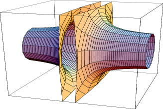
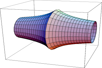
Figure 1: Moduli spaces from 1-loop field theory (left) and supergravity (right).

The plot on the left shows the one-loop corrected moduli space predicted by field theory calculations. At very large values of the non-compact scalar, it tends to flat cylinder with radius proportional to $|e|/\sqrt{N}$. As this $vev$ decreases higher loop corrections are needed. In particular, the one loop calculation diverges at $r=2e^{2}$.

On the other hand, the figure on the right shows the moduli space predicted by supergravity. It also tends to a cylinder with vanishing radius at large values of the non-compact scalar, so it agrees with the $N\rightarrow\infty$ limit of the field theory. It also smooths the divergence of the one loop calculation, which could maybe correspond to a resummation of infinite loops contributions. Strictly speaking, we see from (14) that the supergravity approximation is not valid at $r=0$, where the curvature of our background blows up. In any case, we can still use it as close to the origin as needed by taking $g_{s}N$ large enough.

Finally, we shall make more explicit the relation between the parameters in supergravity ($g_{s}$, $N$ and $l$) and in the field theory ($e$ and $N$). As usual, the number $N$ of D6-branes is the rank of the gauge group. On the other hand, in the supergravity side, a non-zero value for $l$ prevents the radius from diverging as we approach the origin. Nevertheless, it is difficult to make the dictionary more precise. In any case, one can read the gauge coupling for the $U(1)$ degrees of freedom at a certain point of the moduli space by identifying the coefficient in front of the $F^{2}$ term in the DBI action of probe. The result is

$${1\over g_{U(1)}^{2}}=4\pi^{2}\mu_{6}\,g_{s}N^{2}\,(r^{2}+l^{2})$$ (22)

3.3 The noncommutative moduli space

Exactly the same method used to obtain the moduli space of the commutative field theory can be used to study the noncommutative one. In this case we have to use the full NC background (10). The vacuum of the probe brane is the same. This is due to the fact that, in the static gauge, and without exciting the fields on the probe, one can verify that our background satisfies

$$e^{-\Phi^{\Theta}}\sqrt{-\det[G^{\Theta}]}=e^{-\Phi^{\Theta=0}}\sqrt{-\det[G^{\Theta=0}]}\,,\;\;\;\;\;\;\;\;\;\;\;\;\;\;\;\;\;\;C^{\Theta}_{[7]}+B^{\Theta}_{[2]}\wedge C^{\Theta}_{[5]}=C^{\Theta=0}_{[7]}$$ (23)

In superscripts we indicate whether the field is written at finite or at zero value for $\Theta$, and pullbacks are to be understood where needed. Since the DBI lagrangian is unchanged, the supersymmetric loci are still at $\theta=0,\pi$.

When we look for the low energy excitations of the fields on the brane, we find again the same metric on the moduli space. This time, the relevant property of the background is

$$e^{-\Phi^{\Theta}}\sqrt{-\det[G^{\Theta}+B_{[2]}^{\Theta}+2\pi\alpha^{\prime}F_{[2]}]}+2\pi\alpha^{\prime}F_{[2]}\wedge C^{\Theta}_{[5]}=e^{-\Phi^{\Theta=0}}\sqrt{-\det[G^{\Theta=0}+2\pi\alpha^{\prime}F_{[2]}]}$$ (24)

where the equality is to be understood only between the terms which are quadratic in the derivatives on both sides.

Acknowledgements

We are grateful to Jaume Gomis, Jorge Russo, Luca Tagliacozzo and Paul Townsend for useful discussions. This work is partially supported by MCYT FPA, 2001-3598, and CIRIT, GC 2001SGR-00065, and HPRN-CT-2000-00131. T.M. is supported by a grant from the Commissionat per a la Recerca de la Generalitat de Catalunya. J.B. is supported by a grant from Ministerio de Ciencia y Tecnología.

References

- [1] J. M. Maldacena, Adv. Theor. Math. Phys. 2 (1998) 231 [Int. J. Theor. Phys. 38 (1999) 1113] [arXiv:hep-th/9711200]. S. S. Gubser, I. R. Klebanov and A. M. Polyakov, Phys. Lett. B 428 (1998) 105 [arXiv:hep-th/9802109]. E. Witten, Adv. Theor. Math. Phys. 2 (1998) 253 [arXiv:hep-th/9802150].
- [2] J. M. Maldacena and C. Nunez, Int. J. Mod. Phys. A 16 (2001) 822 [arXiv:hep-th/0007018].
- [3] J. M. Maldacena and C. Nunez, Phys. Rev. Lett. 86 (2001) 588 [arXiv:hep-th/0008001]. B. S. Acharya, J. P. Gauntlett and N. Kim, Phys. Rev. D 63 (2001) 106003 [arXiv:hep-th/0011190]. H. Nieder and Y. Oz, JHEP 0103 (2001) 008 [arXiv:hep-th/0011288]. J. P. Gauntlett, N. Kim and D. Waldram, Phys. Rev. D 63 (2001) 126001 [arXiv:hep-th/0012195]. C. Nunez, I. Y. Park, M. Schvellinger and T. A. Tran, JHEP 0104 (2001) 025 [arXiv:hep-th/0103080]. J. D. Edelstein and C. Nunez, JHEP 0104 (2001) 028 [arXiv:hep-th/0103167]. M. Schvellinger and T. A. Tran, JHEP 0106 (2001) 025 [arXiv:hep-th/0105019]. J. M. Maldacena and H. Nastase, JHEP 0109 (2001) 024 [arXiv:hep-th/0105049]. J. P. Gauntlett, N. Kim, S. Pakis and D. Waldram, Phys. Rev. D 65 (2002) 026003 [arXiv:hep-th/0105250]. R. Hernandez, Phys. Lett. B 521 (2001) 371 [arXiv:hep-th/0106055]. J. P. Gauntlett, N. Kim, D. Martelli and D. Waldram, Phys. Rev. D 64 (2001) 106008 [arXiv:hep-th/0106117]. F. Bigazzi, A. L. Cotrone and A. Zaffaroni, Phys. Lett. B 519 (2001) 269 [arXiv:hep-th/0106160]. J. P. Gauntlett and N. Kim, Phys. Rev. D 65 (2002) 086003 [arXiv:hep-th/0109039]. J. Gomis, Nucl. Phys. B 624 (2002) 181 [arXiv:hep-th/0111060]. G. Curio, B. Kors and D. Lust, arXiv:hep-th/0111165. P. Di Vecchia, H. Enger, E. Imeroni and E. Lozano-Tellechea, Nucl. Phys. B 631 (2002) 95 [arXiv:hep-th/0112126]. R. Hernandez and K. Sfetsos, Phys. Lett. B 536 (2002) 294 [arXiv:hep-th/0202135]. J. P. Gauntlett, N. Kim, S. Pakis and D. Waldram, arXiv:hep-th/0202184. U. Gursoy, C. Nunez and M. Schvellinger, JHEP 0206 (2002) 015 [arXiv:hep-th/0203124]. R. Hernandez and K. Sfetsos, arXiv:hep-th/0205099. P. Di Vecchia, A. Lerda and P. Merlatti, arXiv:hep-th/0205204. R. Apreda, F. Bigazzi, A. L. Cotrone, M. Petrini and A. Zaffaroni, Phys. Lett. B 536 (2002) 161 [arXiv:hep-th/0112236]. M. Naka, arXiv:hep-th/0206141. J. D. Edelstein, A. Paredes and A. V. Ramallo, arXiv:hep-th/0207127. R. Hernandez and K. Sfetsos, arXiv:hep-th/0211130. J. D. Edelstein, A. Paredes and A. V. Ramallo, arXiv:hep-th/0211203. J. D. Edelstein, arXiv:hep-th/0211204. J. D. Edelstein, A. Paredes and A. V. Ramallo, arXiv:hep-th/0212139.
- [4] J. Gomis and J. G. Russo, JHEP 0110 (2001) 028 [arXiv:hep-th/0109177]. J. P. Gauntlett, N. w. Kim, D. Martelli and D. Waldram, JHEP 0111 (2001) 018 [arXiv:hep-th/0110034].
- [5] J. Gomis and T. Mateos, Phys. Lett. B 524 (2002) 170 [arXiv:hep-th/0108080].
- [6] M. Bershadsky, C. Vafa and V. Sadov, Nucl. Phys. B 463 (1996) 420 [arXiv:hep-th/9511222].
- [7] A. Hashimoto and N. Itzhaki, Phys. Lett. B 465 (1999) 142 [arXiv:hep-th/9907166]. J. M. Maldacena and J. G. Russo, JHEP 9909 (1999) 025 [arXiv:hep-th/9908134]. M. Alishahiha, Y. Oz and M. M. Sheikh-Jabbari, JHEP 9911 (1999) 007 [arXiv:hep-th/9909215]. D. S. Berman et al., JHEP 0105 (2001) 002 [arXiv:hep-th/0011282].
- [8] H. Larsson, Class. Quant. Grav. 19 (2002) 2689 [arXiv:hep-th/0105083].
- [9] J. Brugues, J. Gomis, T. Mateos and T. Ramirez, JHEP 0210 (2002) 016 [arXiv:hep-th/0207091].
- [10] M. J. Duff, H. Lu and C. N. Pope, Phys. Lett. B 409 (1997) 136 [arXiv:hep-th/9704186].
- [11] I. Affleck, J. A. Harvey and E. Witten, Nucl. Phys. B 206 (1982) 413.
- [12] A. Buchel, A. W. Peet and J. Polchinski, Phys. Rev. D 63 (2001) 044009 [arXiv:hep-th/0008076].
- [13] T. Mateos, J. M. Pons and P. Talavera, arXiv:hep-th/0209150.
- [14] J. de Boer, K. Hori and Y. Oz, Nucl. Phys. B 500 (1997) 163 [arXiv:hep-th/9703100]. O. Aharony, A. Hanany, K. A. Intriligator, N. Seiberg and M. J. Strassler, Nucl. Phys. B 499 (1997) 67 [arXiv:hep-th/9703110].
- [15] A. Salam and E. Sezgin, Nucl. Phys. B 258 (1985) 284.