Parafermionic theory with the symmetry $Z_{5}$.
Vladimir S. Dotsenko⁽¹⁾, Jesper Lykke Jacobsen⁽²⁾ and Raoul Santachiara⁽¹⁾
(1) LPTHE, Université Pierre et Marie Curie, Paris VI
Boîte 126, Tour 16, 1^er étage, 4 place Jussieu, F-75252 Paris Cedex 05, France.
(2) Laboratoire de Physique Théorique et Modèles Statistiques,
Université Paris-Sud, Bâtiment 100, F-91405 Orsay, France.
dotsenko@lpthe.jussieu.fr, jacobsen@ipno.in2p3.fr, santachiara@lpthe.jussieu.fr

Abstract.

A parafermionic conformal theory with the symmetry $Z_{5}$ is constructed, based on the second solution of Fateev-Zamolodchikov for the corresponding parafermionic chiral algebra.

The primary operators of the theory, which are the singlet, doublet 1, doublet 2, and disorder operators, are found to be accommodated by the weight lattice of the classical Lie algebra $B_{2}$. The finite Kac tables for unitary theories are defined and the formula for the conformal dimensions of primary operators is given.

1 Introduction

Extra discrete group symmetries in two-dimensional critical phenomena are naturally realised by parafermionic chiral algebras. The most well-known and widely used parafermionic conformal theory is due to Fateev and Zamolodchikov [1]. It describes, in particular, the self-dual fixed points of a particular lattice model with $Z_{N}$ symmetry [1,2].

In terms of the associativity constraint for physically consistent chiral algebras, the parafermions of the theory [1] represent the first solution, with the minimal possible values of the conformal dimensions (or spins) of the parafermionic currents. In this solution the central charge of the corresponding Virasoro algebra is a function of $N$ only, i.e., for each $N$ of the group $Z_{N}$ there is just one conformal theory, with a given, fixed value $c_{N}$ of the central charge.

These same authors gave in the Appendix of Ref. [1] a second solution of the associative parafermionic chiral algebra, with the next allowed values of the spins of the parafermions. In the second $Z_{N}$ symmetric solution the central charge remains a free parameter, for each $N$.

The case $N=2$ of this second solution corresponds to the superconformal theory. The conformal theory corresponding to the second solution with $Z_{3}$ symmetry has been fully constructed by Fateev and Zamolodchikov in a subsequent work, Ref. [3]. It produces an infinite set of conformal theories which are selected by applying the degeneracy condition to the representations generated by physical fields, similar to the case of minimal models of purely conformal (non-extended) conformal field theory. This infinite set of conformal theories was supposed [3] to correspond to higher, multicritical fixed points of physical statistical systems with the symmetry $Z_{3}$. And in fact, the first theory in this set (the one with the least value of the central charge) was shown to correspond to the tricritical Potts model.

For the second associative solution of the chiral algebra [1], the conformal theories with $N>3$ (i.e., with symmetries $Z_{4}$, $Z_{5}$, $Z_{6}$ etc.) have not been constructed so far. The purpose of our present work is to build the corresponding theories. In particular, we shall define the Kac formula giving the conformal dimensions of physical (primary) fields, which realise degenerate representations of the corresponding parafermionic chiral algebras.

The first of these theories, the one of $N=4$, turns out to be trivial in the sense that it factorises into two independent superconformal chiral algebras, with fields of dimensions $2$ and $3/2$.

The first new theory is therefore that of $Z_{5}$. This theory in itself turns out to be so rich, and also representative for the whole class (whilst being the simplest at the same time), that it appeared reasonable for us to present it separately, in all the details. The present paper is therefore devoted to the theory $Z_{5}$, and generalisations will be given in a following work [4].

One extra result which we have used in our construction is that the central charge for the second solution of the $Z_{N}$ parafermionic algebra agrees with that of the coset [5]

$$\frac{SO_{k}(N)\times SO_{2}(N)}{SO_{k+2}(N)},$$ (1.1)

which is

$$c = (N-1)\left(1-\frac{N(N-2)}{p(p+2)}\right),$$ (1.2)

$$p = N-2+k.$$ (1.3)

In the construction of the representation theory of the parafermionic algebra this observation turns out to be extremely useful.

Our paper is organised as follows. In Section 2 we review some technical details on the second associative solution of the chiral algebra as found in Ref. [1]. We then specialise to the case of $Z_{5}$. The structure of the representation modules of the various physical operators (singlets, doublets, disorder operators) are fixed. We present explicit calculations of the first degeneracies in these modules. The resulting conformal dimensions, and the levels on which singular states are found, serve as initial conditions for dressing the entire theory. In Section 3 we give the Kac formula of the theory. We give the boundary terms corresponding to the various sectors of the theory.

The general question of determining the appropriate sector label for each operator in the theory is addressed in Section 4. We give a first argument, based on fusion rules and an assumed Coulomb gas construction. Some aspects of this argument are then verified by considering differential and characteristic equations for three-point functions. We also give the general formula for the eigenvalues of the parafermionic zero modes for the disorder operators. The conclusions are given in Section 5.

Four appendices deal with technical points of the calculations.

2 Parafermionic algebras in different sectors. First degeneracies

The operator product expansions of chiral fields within the second solution of the $Z_{N}$ symmetric parafermionic algebra is given in Appendix A of Ref. [1]. They take the form

$$\Psi^{q}(z)\Psi^{q^{\prime}}(z^{\prime}) = \frac{\lambda^{q,q^{\prime}}_{q+q^{\prime}}}{(z-z^{\prime})^{\Delta_{q}+\Delta_{q^{\prime}}-\Delta_{q+q^{\prime}}}}$$

$$\times \left\{\Psi^{q+q^{\prime}}(z^{\prime})+(z-z^{\prime})\frac{\Delta_{q+q^{\prime}}+\Delta_{q}-\Delta_{q^{\prime}}}{2\Delta_{q+q^{\prime}}}\partial_{z^{\prime}}\Psi^{q+q^{\prime}}(z^{\prime})+\ldots\right\},\quad q+q^{\prime}\neq 0$$

$$\Psi^{q}(z)\Psi^{-q}(z^{\prime}) = \frac{1}{(z-z^{\prime})^{2\Delta_{q}}}\left\{1+(z-z^{\prime})^{2}\frac{2\Delta_{q}}{c}T(z^{\prime})+\ldots\right\}$$ (2.2)

Here the structure constants $\lambda_{q+q^{\prime}}^{q,q^{\prime}}$ and the central charge $c$ (of the Virasoro algebra) are given by the expressions:

$$(\lambda^{q,q^{\prime}}_{q+q^{\prime}})^{2} = \frac{\Gamma(q+q^{\prime}+1)\Gamma(N-q+1)\Gamma(N-q^{\prime}+1)}{\Gamma(q+1)\Gamma(q^{\prime}+1)\Gamma(N-q-q^{\prime}+1)\Gamma(N+1)}$$ (2.3)

$$\times \frac{\Gamma(q+q^{\prime}+v)\Gamma(N+v-q)\Gamma(N+v-q^{\prime})\Gamma(v)}{\Gamma(N+v-q-q^{\prime})\Gamma(q+v)\Gamma(q^{\prime}+v)\Gamma(N+v)},$$

$$c = \frac{4(N-1)(N+v-1)v}{(N+2v)(N+2v-2)}.$$ (2.4)

The dimensions of the fields $\{\Psi^{q}(z)\}$ have the following form:

$$\Delta_{q}=\Delta_{N-q}=\frac{2q(N-q)}{N}.$$ (2.5)

Note in particular that the field $\Psi^{-q}$ in (2.2) is assumed to have dimension $\Delta_{N-q}$, in the sense that the indices $q$ referring to the $Z_{N}$ charge are always defined modulo $N$. Thus,

$$\Psi^{N-q}\equiv\Psi^{-q}\equiv(\Psi^{q})^{+},\quad\Delta_{N-q}\equiv\Delta_{-q}.$$ (2.6)

In the expressions (2.3)–(2.4) $v$ is a free parameter, which was chosen in [1] to parametrise this solution. If one defines

$$v=2k$$ (2.7)

then the expression (2.4) for the central charge $c$ could also be represented as in (1.2), making connection to the coset (1.1) [5].

From now on we specialise in this paper to the case $N=5$, for the reasons given in the Introduction. In this case the $Z_{5}$ charge $q$ takes the values $0,\pm 1,\pm 2,$ and we have the following parafermionic fields:

$$\Psi^{\pm 1}(z),\quad\Psi^{\pm 2}(z).$$ (2.8)

Together with the identity and the stress-energy operator $T(z)$ these fields make a closed operator algebra, given by Eqs. (2)–(2.2). Their dimensions are

$$\Delta_{1}=\frac{8}{5},\quad\Delta_{2}=\frac{12}{5}$$ (2.9)

according to Eq. (2.5).

On the side of the representation fields, primary fields of the algebra (2)–(2.2), we should expect the singlet operators:

$$\Phi^{0}(z,\bar{z})\quad(q=0)$$ (2.10)

the doublet 1 operators:

$$\Phi^{\pm 1}(z,\bar{z})\quad(q=\pm 1)$$ (2.11)

and the doublet 2 operators:

$$\Phi^{\pm 2}(z,\bar{z})\quad(q=\pm 2).$$ (2.12)

In addition to these usual representations of the $Z_{5}$ group we expect the spectrum to include a quintuplet (5-plet) of $Z_{2}$ disorder operators:

$$\{R^{a}(z,\bar{z}),\quad a=1,2,3,4,5\}.$$ (2.13)

The presence of disorder operators reflects the fact that the theory is, in fact, invariant under a larger group than $Z_{5}$, viz. the dihedral group $D_{5}$. This group includes, in addition to $Z_{5}$, also the $Z_{2}$ reflections with respect to the five axes shown in Fig. 1.

Figure 1: The action of the parafermionic current $\Psi^{k}$ can be represented pictorially as a $2\pi k/5$ rotation of a pentagon. A quintuplet of disorder operators augments the cyclic symmetry to a dihedral one, each operator corresponding to the $Z_{2}$ reflection with respect to an axis passing through one of the vertices of the pentagon. The labeling of the five axes, as shown on the figure, is also used to label the corresponding disorder operators.

This higher symmetry stems from the fact that in the solution (2)–(2.5) everything is symmetric with respect to the $Z_{N}$ charge conjugation:

$$q\rightarrow N-q.$$ (2.14)

(For the structure constants $(\lambda^{q,q^{\prime}}_{q+q^{\prime}})^{2}$ in Eq. (2.3) the demonstration requires a little algebra with products.)

The disorder fields have previously been shown to be in the spectrum of the $Z_{3}$ theory, second solution, as constructed in Ref. [3]. They appear as triplet representations in this case. The disorder fields also appear in the first solution [1] (for the case of general $Z_{N}$), and have been defined and fully treated in Ref. [6].

One could object that the disorder fields $\{R_{a}(z,\bar{z})\}$ in Eq. (2.13) are on a somewhat different footing than the standard (singlet and doublet) representation fields. Namely, the disorder fields complete the cyclic group $Z_{5}$, as generated by $1=\Psi^{0}(z)$, $\Psi^{\pm 1}(z)$ and $\Psi^{\pm 2}(z)$, to the dihedral group $D_{5}$. However, there is a crucial difference between the $\Psi$ and the $R$ fields. The first are chiral, or holomorphic, whilst the latter are non-chiral, like the rest of the representation operators. So despite of the fact that the symmetry of the theory is $D_{5}$, not all of the elements in the dihedral group are represented in the chiral algebra but only those of the biggest abelian subalgebra, $Z_{5}$. The rest of the group elements find themselves in the representation space, as disorder operators.

This is at least the structure of the present theory, and of the theory $Z_{3}$ in Ref. [3].

Summarising, we expect that the representation space of the theory $Z_{5}$ can be divided into singlet, doublet 1, doublet 2, and disorder operators, cf. Eqs. (2.10)–(2.13).

It is already a standard point that the spectrum, for a given chiral algebra with a free parameter (the central charge (2.4), or the parameter $v$), is to be defined by the degeneracy condition of the representations. The reasoning why this is so can be given in various ways, for example by demanding the closure of the operator algebra of primary (physical) fields.

To define the spectrum of dimensions of singlets, doublets, and disorder operators, we have to define the representations of the chiral algebra in the corresponding sectors. One then constructs the modules induced by the various primary fields, and demands their degeneracy.

As usual, it will be sufficient to analyse directly the degeneracies on the first few levels in the modules. The physical operators defined in this way become the basic ones in the Kac table. Using these basic fields we shall be able, in the following Sections, to define the whole set, the Kac table and the formula for the dimensions.

2.1 Structure of the representation modules

The level structure of the modules induced by the singlets and by the two types of doublets can be defined as follows. We first place the chiral fields, i.e., the parafermions $\Psi^{\pm 1}(z)$, $\Psi^{\pm 2}(z)$ as well as the stress-energy operator $T(z)$, in the module of identity. The levels of the various operators in this module correspond to their conformal dimensions: $\Delta_{\pm 1}=8/5$ and $\Delta_{\pm 2}=12/5$. This partially filled identity module is shown in Fig. 2. To make apparent the crucial role played by the $Z_{5}$ charge $q$, we depict the modules by separating the various charge sectors horizontally.

Figure 2: The position of the parafermionic currents in the identity module. The horizontal axis shows the $Z_{5}$ charge $q$. The vertical axis gives the level of a given state, here with respect to the identity operator placed at the summit of the diagram.

Next, the level spacing within each charge sector (along a given vertical line on the figure) should be equal to 1, as the monodromy of the $\Psi$ fields is abelian. This is so with respect to the identity operator, and, more generally, with respect to the singlet and doublet operators forming the usual representations of the abelian group $Z_{5}$. So we can complete the levels in the identity module as shown in Fig. 3. The states below $I$ and above $\Psi^{\pm 1}$, on levels 2/5, 3/5, 1, and 7/5 are actually empty. They will however become occupied when the identity operator $I$, placed at the summit of the module, is replaced by a more general singlet state, $\Phi^{0}$.

Figure 3: Completion of the identity module. Each state is shown as a filled circle.

We can now read off from Fig. 3 the level structure of the doublet 1 (with $\Phi^{\pm 1}$ at the summit) and the doublet 2 (with $\Phi^{\pm 2}$ at the summit) modules by inspecting their corresponding submodules in Fig. 3. For instance, for the doublet 1 we should consider the two states in Fig. 3 on level 3/5 as being at the summit, i.e., by imposing the levels above these states to be empty. Then, everything has to be shifted upwards by 3/5, putting these states at level 0. Proceeding in this way one obtains the level structure of the modules for a singlet, a doublet 1, and a doublet 2 operator, as shown in Figs. 4, 5 and 6. The consistency of these manipulations is ensured by the associativity of the algebra of $\Psi$ fields.

Figure 4: Representation module of a singlet operator. Arrows depict (some of) the possible actions by the parafermionic mode operators (with an appropriate change of the $Z_{5}$ charge $q$) and by the Virasoro generators (with no change in $q$).

Figure 5: Representation module of a doublet of operators of charge $q=\pm 1$, henceforth referred to as doublet 1. Note the existence of a zero mode linking the two states at the summit of the diagram.

Figure 6: Representation module of a doublet 2 operator. The two states at the summit are linked by a zero mode.

In accordance with the structure of the modules, as depicted in Figs. 4–6, the local developments of the chiral fields $\Psi$ in the basis of the representation fields, $\Phi^{0}$, $\Phi^{\pm 1}$ and $\Phi^{\pm 2}$, should be of the forms given below.

In the singlet basis one has:

$$\Psi^{\pm 1}(z)\Phi^{0}(0) = \sum_{n}\frac{1}{(z)^{\Delta_{1}-\frac{3}{5}+n}}A^{\pm 1}_{-\frac{3}{5}+n}\Phi^{0}(0),$$

$$A^{\pm 1}_{-\frac{3}{5}+n}\Phi^{0}(0) = 0,\quad n>0$$ (2.15)

$$\Psi^{\pm 2}(z)\Phi^{0}(0) = \sum_{n}\frac{1}{(z)^{\Delta_{2}-\frac{2}{5}+n}}A^{\pm 2}_{-\frac{2}{5}+n}\Phi^{0}(0),$$

$$A^{\pm 2}_{-\frac{2}{5}+n}\Phi^{0}(0) = 0,\quad n>0.$$ (2.16)

The fact that positive-index mode operators annihilate $\Psi^{0}(0)$ is the usual highest-weight condition, expressing the fact that we are trying to make the representation fields primary with respect to the chiral algebra. Conversely, one gets:

$$A^{\pm 1}_{-\frac{3}{5}+n}\Phi^{0}(0) = \frac{1}{2\pi i}\oint_{C_{0}}{\rm d}z\,(z)^{\Delta_{1}-\frac{3}{5}+n-1}\Psi^{\pm 1}(z)\Phi^{0}(0),$$ (2.17)

$$A^{\pm 2}_{-\frac{2}{5}+n}\Phi^{0}(0) = \frac{1}{2\pi i}\oint_{C_{0}}{\rm d}z\,(z)^{\Delta_{2}-\frac{2}{5}+n-1}\Psi^{\pm 2}(z)\Phi^{0}(0).$$ (2.18)

The arrows in Figs. 4–6 represent the actions of the mode operators $A^{\pm 1}_{\mu}$ and $A^{\pm 2}_{\mu}$. For the sake of clarity not all possible arrows are shown. In particular, we do not show the upwards arrows which would represent the action on a descendent state. The “gaps” in the modules, i.e., the level of the first descendents, show up in the fractional shifts of the indices of the operators $A^{\pm 1}_{\mu}$ and $A^{\pm 2}_{\mu}$ (e.g., $\mu=-3/5+n$ in Eq. (2.17), etc.).

In a similar way, for the doublet 1 one gets:

$$\Psi^{\pm 1}(z)\Phi^{\mp 1}(0) = \sum_{n}\frac{1}{(z)^{\Delta_{1}-\frac{2}{5}+n}}A^{\pm 1}_{-\frac{2}{5}+n}\Phi^{\mp 1}(0),$$ (2.19)

$$\Psi^{\pm 1}(z)\Phi^{\pm 1}(0) = \sum_{n}\frac{1}{(z)^{\Delta_{1}-\frac{4}{5}+n}}A^{\pm 1}_{-\frac{4}{5}+n}\Phi^{\pm 1}(0),$$ (2.20)

$$\Psi^{\pm 2}(z)\Phi^{\mp 1}(0) = \sum_{n}\frac{1}{(z)^{\Delta_{2}+n}}A^{\pm 2}_{n}\Phi^{\mp 1}(0),$$ (2.21)

$$\Psi^{\pm 2}(z)\Phi^{\pm 1}(0) = \sum_{n}\frac{1}{(z)^{\Delta_{2}-\frac{4}{5}+n}}A^{\pm 2}_{-\frac{4}{5}+n}\Phi^{\pm 1}(0).$$ (2.22)

We remark that the action of $\Psi^{\pm 2}(z)$ on $\Phi^{\mp 1}(0)$ in Eq. (2.21) involves a zero mode $A^{\pm 2}_{0}$, which acts between the states $\Phi^{\pm 1}(0)$ at the summit:

$$A^{\mp 2}_{0}\Phi^{\pm 1}(0)=h_{2,1}\Phi^{\mp 1}(0).$$ (2.23)

The index of the eigenvalue $h_{2,1}$ refers to the indices of $A$ and $\Phi$. Another zero mode appears in the action of $\Psi^{\pm 1}(z)$ on $\Phi^{\pm 2}(0)$:

$$A^{\pm 1}_{0}\Phi^{\pm 2}(0)=h_{1,2}\Phi^{\mp 2}(0).$$ (2.24)

(The corresponding expansion, in the basis of $\Phi^{\pm 2}(0)$, is given below.) The eigenvalues $h$ in Eqs. (2.23)–(2.24) characterise the representations, in addition to the values of the conformal dimensions of the fields $\Phi^{\pm 1}$, $\Phi^{\pm 2}$ (which are the eigenvalues of the Virasoro zero mode $L_{0}$).

The relations which are the inverse of Eqs. (2.19)–(2.22) read:

$$A^{\pm 1}_{-\frac{2}{5}+n}\Phi^{\mp 1}(0) = \frac{1}{2\pi i}\oint_{C_{0}}{\rm d}z\,(z)^{\Delta_{1}-\frac{3}{5}+n-1}\Psi^{\pm 1}(z)\Phi^{\mp 1}(0),$$ (2.25)

$$A^{\pm 1}_{-\frac{4}{5}+n}\Phi^{\pm 1}(0) = \frac{1}{2\pi i}\oint_{C_{0}}{\rm d}z\,(z)^{\Delta_{1}-\frac{4}{5}+n-1}\Psi^{\pm 1}(z)\Phi^{\pm 1}(0),$$ (2.26)

$$A^{\pm 2}_{n}\Phi^{\mp 1}(0) = \frac{1}{2\pi i}\oint_{C_{0}}{\rm d}z\,(z)^{\Delta_{2}+n-1}\Psi^{\pm 2}(z)\Phi^{\mp 1}(0),$$ (2.27)

$$A^{\pm 2}_{-\frac{4}{5}+n}\Phi^{\pm 1}(0) = \frac{1}{2\pi i}\oint_{C_{0}}{\rm d}z\,(z)^{\Delta_{2}-\frac{4}{5}+n-1}\Psi^{\pm 2}(z)\Phi^{\pm 1}(0).$$ (2.28)

Finally, for the doublet 2 one gets the expansions:

$$\Psi^{\pm 1}(z)\Phi^{\mp 2}(0) = \sum_{n}\frac{1}{(z)^{\Delta_{1}-\frac{1}{5}+n}}A^{\pm 1}_{-\frac{1}{5}+n}\Phi^{\mp 2}(0),$$ (2.29)

$$\Psi^{\pm 1}(z)\Phi^{\pm 2}(0) = \sum_{n}\frac{1}{(z)^{\Delta_{1}+n}}A^{\pm 1}_{n}\Phi^{\pm 2}(0),$$ (2.30)

$$\Psi^{\pm 2}(z)\Phi^{\mp 2}(0) = \sum_{n}\frac{1}{(z)^{\Delta_{2}-\frac{3}{5}+n}}A^{\pm 2}_{-\frac{3}{5}+n}\Phi^{\mp 2}(0),$$ (2.31)

$$\Psi^{\pm 2}(z)\Phi^{\pm 2}(0) = \sum_{n}\frac{1}{(z)^{\Delta_{2}-\frac{1}{5}+n}}A^{\pm 2}_{-\frac{1}{5}+n}\Phi^{\pm 2}(0),$$ (2.32)

the inverse relations being:

$$A^{\pm 1}_{-\frac{1}{5}+n}\Phi^{\mp 2}(0) = \frac{1}{2\pi i}\oint_{C_{0}}{\rm d}z\,(z)^{\Delta_{1}-\frac{1}{5}+n-1}\Psi^{\pm 1}(z)\Phi^{\mp 2}(0),$$ (2.33)

$$A^{\pm 1}_{n}\Phi^{\pm 2}(0) = \frac{1}{2\pi i}\oint_{C_{0}}{\rm d}z\,(z)^{\Delta_{1}+n-1}\Psi^{\pm 1}(z)\Phi^{\pm 2}(0),$$ (2.34)

$$A^{\pm 2}_{-\frac{3}{5}+n}\Phi^{\mp 2}(0) = \frac{1}{2\pi i}\oint_{C_{0}}{\rm d}z\,(z)^{\Delta_{2}-\frac{3}{5}+n-1}\Psi^{\pm 2}(z)\Phi^{\mp 2}(0),$$ (2.35)

$$A^{\pm 2}_{-\frac{1}{5}+n}\Phi^{\pm 2}(0) = \frac{1}{2\pi i}\oint_{C_{0}}{\rm d}z\,(z)^{\Delta_{2}-\frac{1}{5}+n-1}\Psi^{\pm 2}(z)\Phi^{\pm 2}(0).$$ (2.36)

2.2 Degeneracy of the modules

Having defined the mode operators, $A^{\pm 1}_{\mu}$ and $A^{\pm 2}_{\mu}$, we now turn to the problem of degeneracies in the modules.

To analyse the degeneracies, we shall need to compute various matrix elements of the mode operators. To this end, we shall make extensive use of the commutation relations of the mode operators, in the various sectors. For convenience, we have listed the complete set of commutation relations in Appendix A: these are all obtained in a way analogous to that used in Refs. [1,3]. We also exemplify in Appendix A the computation of some of the matrix elements needed in the subsequent analysis.

2.2.1 Doublet 1

For the doublet 1 module, depicted on Fig. 5, we begin by imposing degeneracy at level $2/5$. Forming the linear combination

$$\chi^{0}_{-\frac{2}{5}}=aA^{1}_{-\frac{2}{5}}\Phi^{-1}+bA^{-1}_{-\frac{2}{5}}\Phi^{1},$$ (2.37)

we wish to make it into a primary operator, i.e., to ensure that it is annihilated upon action by positive index mode operators. In this case it will be sufficient to verify that

$$A^{1}_{+\frac{2}{5}}\chi^{0}_{-\frac{2}{5}}=0\quad\mbox{and}\quad A^{-1}_{+\frac{2}{5}}\chi^{0}_{-\frac{2}{5}}=0.$$ (2.38)

The others arrows going upwards in Fig. 5 will be zero for trivial reasons.

The conditions (2.38) for the state (2.37) can be rewritten as:

$$aA^{1}_{\frac{2}{5}}A^{1}_{-\frac{2}{5}}\Phi^{-1}+bA^{1}_{\frac{2}{5}}A^{-1}_{-\frac{2}{5}}\Phi^{1} = 0,$$

$$aA^{-1}_{\frac{2}{5}}A^{1}_{-\frac{2}{5}}\Phi^{-1}+bA^{-1}_{\frac{2}{5}}A^{-1}_{-\frac{2}{5}}\Phi^{1} = 0,$$ (2.39)

where, obviously, $A^{1}_{\frac{2}{5}}A^{1}_{-\frac{2}{5}}\Phi^{-1}\propto\Phi^{1}$ etc. It is convenient to define matrix elements $\mu$ by

$$A^{1}_{\frac{2}{5}}A^{1}_{-\frac{2}{5}}\Phi^{-1} = \mu^{(1,1;-1)}_{\frac{2}{5},-\frac{2}{5}}\Phi^{1},$$ (2.40)

$$A^{1}_{\frac{2}{5}}A^{-1}_{-\frac{2}{5}}\Phi^{1} = \mu^{(1,-1;1)}_{\frac{2}{5},-\frac{2}{5}}\Phi^{1},$$ (2.41)

$$A^{-1}_{\frac{2}{5}}A^{1}_{-\frac{2}{5}}\Phi^{-1} = \mu^{(-1,1;-1)}_{\frac{2}{5},-\frac{2}{5}}\Phi^{-1},$$ (2.42)

$$A^{-1}_{\frac{2}{5}}A^{-1}_{-\frac{2}{5}}\Phi^{1} = \mu^{(-1,-1;1)}_{\frac{2}{5},-\frac{2}{5}}\Phi^{-1}.$$ (2.43)

By the $Z_{2}$ reflection symmetry $(q\leftrightarrow-q)$ we have

$$\mu^{(1,1;-1)} = \mu^{(-1,-1;1)},$$ (2.44)

$$\mu^{(1,-1;1)} = \mu^{(-1,1;-1)}.$$ (2.45)

To compute the remaining two matrix elements in Eq. (2.39) we need the commutation relations of the mode operators $A^{\pm 1}_{\mu}$. In Appendix A it is shown that

$$\mu^{(1,1;-1)}_{\frac{2}{5},-\frac{2}{5}} = \lambda^{1,1}_{2}h_{2,1},$$ (2.46)

$$\mu^{(1,-1;1)}_{\frac{2}{5},-\frac{2}{5}} = -\frac{2}{25}+\frac{2\Delta_{1}}{c}\Delta_{\Phi^{1}}.$$ (2.47)

Here, $\lambda^{1,1}_{2}$ is one of the structure constants (2.3) of the chiral algebra (2) and $h_{2,1}$ is the eigenvalue of $\Phi^{\mp 1}$ with respect to the zero mode $A^{\pm 2}$, as defined in Eq. (2.23). Finally, $\Delta_{1}=8/5$ is the dimension of $\Psi^{\pm 1}$, and $\Delta_{\Phi^{1}}$ is the as yet unknown dimension of the operator $\Phi^{\pm 1}$.

A non-trivial solution of the system (2.39) exists provided that

$$\left|\begin{array}[]{cc}\mu^{(1,1;-1)}&\mu^{(1,-1;1)}\\ \mu^{(-1,1;-1)}&\mu^{(-1,-1,1)}\end{array}\right|=0,$$ (2.48)

from which one obtains:

$$\left(\lambda^{1,1}_{2}h_{2,1}\right)^{2}=\left(-\frac{2}{25}+\frac{2}{5c}\Delta_{\Phi^{1}}\right)^{2}.$$ (2.49)

We recall that, for a given operator $\Phi^{1}$ or $\Phi^{-1}$, we need to determine both the eigenvalue $h_{2,1}$ and the dimension $\Delta_{\Phi^{1}}$. By imposing degeneracy at level 2/5, we have obtained Eq. (2.49), which defines $h_{2,1}$ as a function of $\Delta_{\Phi^{1}}$ and $c$. (Note also that the structure constant $\lambda^{1,1}_{2}$ is a function of $c$, by Eqs. (2.3)–(2.4).)

In conclusion, degeneracy at level 2/5 is not sufficient to define also $\Delta_{\Phi^{1}}$ (as a function of $c$). We have two unknowns, $h_{2,1}$ and $\Delta_{\Phi^{1}}$. So we need one more constraint, in addition to that in Eq. (2.49).

We shall therefore require that the doublet 1 module be degenerate also at level 4/5. This is obtained by demanding the degeneracy of the state

$$\chi^{2}_{-\frac{4}{5}}=\tilde{a}A^{1}_{-\frac{4}{5}}\Phi^{1}+\tilde{b}A^{-2}_{-\frac{4}{5}}\Phi^{-1}.$$ (2.50)

The reason for considering a linear combination of two states only is that the “indirect” descendent at level 4/5, obtained by descending through the state which remains at level 2/5 after imposing the degeneracy constraint at that level, is linearly dependent on the direct descendents. More precisely, by using the mode operator algebra given in Appendix A, one finds (in Appendix A) that

$$A^{2}_{-\frac{2}{5}}A^{1}_{-\frac{2}{5}}\Phi^{-1}=A^{2}_{-\frac{2}{5}}A^{-1}_{-\frac{2}{5}}\Phi^{1}$$ (2.51)

is linearly dependent on the states

$$A^{1}_{-\frac{4}{5}}\Phi^{1}\quad\mbox{and}\quad A^{-2}_{\frac{4}{5}}\Phi^{-1}.$$ (2.52)

(In Eq. (2.51) we have used the linear dependence resulting from the degeneracy at level 2/5.)

The degeneracy of the state (2.50) takes the form

$$\left|\begin{array}[]{cc}\mu^{(-1,1;1)}_{\frac{4}{5},-\frac{4}{5}}&\mu^{(-1,-2;-1)}_{\frac{4}{5},-\frac{4}{5}}\\ \mu^{(2,1;1)}_{\frac{4}{5},-\frac{4}{5}}&\mu^{(2,-2,-1)}_{\frac{4}{5},-\frac{4}{5}}\end{array}\right|=0,$$ (2.53)

involving the following matrix elements (see Appendix A for details):

$$A^{-1}_{\frac{4}{5}}A^{1}_{-\frac{4}{5}}\Phi^{1} = \left(\frac{3}{25}+\frac{2\Delta_{1}}{c}\Delta_{\Phi^{1}}\right)\Phi^{1}\equiv\mu^{(-1,1;1)}_{\frac{4}{5},-\frac{4}{5}}\Phi^{1},$$ (2.54)

$$A^{-1}_{\frac{4}{5}}A^{2}_{-\frac{4}{5}}\Phi^{1} = \lambda^{21}_{-2}h_{2,1}\Phi^{1}\equiv\mu^{(-1,-2;-1)}_{\frac{4}{5},-\frac{4}{5}}\Phi^{1},$$ (2.55)

$$A^{2}_{\frac{4}{5}}A^{1}_{-\frac{4}{5}}\Phi^{1} = \lambda^{21}_{-2}h_{2,1}\Phi^{1}\equiv\mu^{(-2,1;1)}_{\frac{4}{5},-\frac{4}{5}}\Phi^{1},$$ (2.56)

$$A^{2}_{\frac{4}{5}}A^{-2}_{-\frac{4}{5}}\Phi^{1} = \left(\frac{4}{(\lambda^{1,1}_{2})^{2}}\left[\frac{4}{5}y^{2}-\frac{2\Delta_{1}}{c}(\Delta_{\Phi^{1}}+\frac{2}{5})y\right]+\frac{9}{5(\lambda^{1,1}_{2})^{2}}y^{2}+\frac{3}{2}y\right)\Phi^{-1}$$ (2.57)

$$\equiv \mu^{(2,-2;-1)}_{\frac{4}{5},-\frac{4}{5}}\Phi^{-1},$$

where

$$y=\lambda^{1,1}_{2}h_{2,1}=-\frac{2}{25}+\frac{2\Delta_{1}}{c}\Delta_{\Phi^{1}}.$$ (2.58)

The solutions of Eq. (2.53), with the ingredients (2.54)–(2.57) as well as Eq. (2.49), have a rather simple form, in spite of its appearances. They can be presented as:

$$\Delta^{(1)}_{\Phi^{1}} = \frac{3}{5}\,\frac{p+5}{p},\quad\Delta^{(2)}_{\Phi^{1}}=\frac{3}{5}\,\frac{p-3}{p+2},$$ (2.59)

$$\Delta^{(3)}_{\Phi^{1}} = \frac{1}{10}\,\frac{p^{2}+2p-15}{p(p+2)},$$ (2.60)

where the parameter $p$ has been defined in Eq. (1.3). For $N=5$,

$$p=3+k=3+\frac{v}{2}$$ (2.61)

where $v$ is the parameter in the solution (2)-(2.5) of the chiral algebra; we recall from Eq. (2.7) that $v=2k$.

By introducing the parameters

$$\alpha^{2}_{+}=\frac{p+2}{p},\quad\alpha^{2}_{-}=\frac{p}{p+2}$$ (2.62)

which are suggestive from the formula for the central charge (1.2), the solutions for the dimensions in Eqs. (2.59)–(2.61) take the form

$$\Delta^{(1)}_{\Phi^{1}} = \frac{3}{2}\alpha^{2}_{+}-\frac{9}{10},\qquad\Delta^{(2)}_{\Phi^{1}}=\frac{3}{2}\alpha^{2}_{-}-\frac{9}{10},$$ (2.63)

$$\Delta^{(3)}_{\Phi^{1}} = -\frac{3}{8}(\alpha^{2}_{+}+\alpha^{2}_{-})+\frac{17}{20}.$$ (2.64)

We shall defer to the next section further discussion on the significance of the solutions (2.63)–(2.64).

We state once again that in the $Z_{5}$ theory the modules have to be doubly degenerate, on two levels simultaneously, to reach the goal that the dimension of the primary field gets fixed as a function of $c$.

2.2.2 Doublet 2

The module of $\Phi^{\pm 2}$, shown in Fig. 6, has its first descendents at level 1/5, with $q=\pm 1$. We could consider one side, $q=-1$ for instance, because what is constructed for $q=-1$ will also be confirmed by the algebra for $q=+1$, due to the $Z_{2}$ reflection symmetry.

At level 1/5 it would appear that there are two states:

$$A^{1}_{-\frac{1}{5}}\Phi^{-2}\quad\mbox{and}\quad A^{2}_{-\frac{1}{5}}\Phi^{2}.$$ (2.65)

However, it turns out that they are proportional to one another. Indeed, by the commutation relation $\{\Psi^{1},\Psi^{1}\}\Phi^{2}$ (see Appendix A) with $n=m=0$, one gets:

$$\lambda^{1,1}_{2}A^{2}_{-\frac{1}{5}}\Phi^{2} = 2A^{1}_{-\frac{1}{5}}A^{1}_{0}\Phi^{2}=2A^{1}_{-\frac{1}{5}}h_{1,2}\Phi^{-2},$$ (2.66)

$$\lambda^{1,1}_{2}A^{2}_{-\frac{1}{5}}\Phi^{2} = 2h_{1,2}A^{1}_{-\frac{1}{5}}\Phi^{-2},$$ (2.67)

where the number $h_{1,2}$ is the zero mode eigenvalue, yet to be fixed.

With this simplification, in order to have a degeneracy at level 1/5, it suffices to require that the state

$$\chi^{-1}_{-\frac{1}{5}}=A^{1}_{-\frac{1}{5}}\Phi^{-2}$$ (2.68)

be primary. Also, it is sufficient to require that it be annihilated by $A^{-1}_{+\frac{1}{5}}$ only, and not by both $A^{-1}_{+\frac{1}{5}}$ and $A^{2}_{+\frac{1}{5}}$. The algebraic reason for this follows from a relation analogous to Eq. (2.67), but for positive index mode operators.

We therefore require that

$$A^{-1}_{\frac{1}{5}}A^{1}_{-\frac{1}{5}}\Phi^{-2}=0,$$ (2.69)

and by means of the commutation relation $\{\Psi^{1},\Psi^{-1}\}\Phi^{-2}$ with $n=m=0$

$$\left(A^{1}_{0}A^{-1}_{0}+A^{-1}_{\frac{1}{5}}A^{1}_{-\frac{1}{5}}\right)\Phi^{-2}=\left(-\frac{3}{25}+\frac{2\Delta_{1}}{c}\Delta_{\Phi^{2}}\right)\Phi^{-2}$$ (2.70)

this takes the form

$$\left(h_{1,2}\right)^{2}=-\frac{3}{25}+\frac{2\Delta_{1}}{c}\Delta_{\Phi^{2}}.$$ (2.71)

If we impose the condition (2.71), the state (2.68) can be put equal to zero, thus reducing the module. As a consequence of the proportionality (2.67) the second state in Eq. (2.65) will then also vanish. Thus, after this reduction, level 1/5 will be completely degenerate, or empty.

Analogous to the case of doublet 1, the constraint (2.71) only defines $(h_{1,2})^{2}$ as a function of $\Delta_{\Phi^{2}}$ and $c$. We therefore turn to level 3/5.

By the commutation relation $\{\Psi^{1},\Psi^{1}\}\Phi^{-2}$ with $n=m=0$ we have

$$2A^{1}_{-\frac{2}{5}}A^{1}_{-\frac{1}{5}}\Phi^{-2}=\lambda^{1,1}_{2}A^{2}_{-\frac{3}{5}}\Phi^{-2}.$$ (2.72)

Since now $A^{1}_{-\frac{1}{5}}\Phi^{-2}=0$, by the previous degeneracy, one obtains

$$A^{2}_{-\frac{3}{5}}\Phi^{-2}=0.$$ (2.73)

Similarly, because of $A^{-1}_{-\frac{1}{5}}\Phi^{2}=0$, one gets

$$A^{-2}_{-\frac{3}{5}}\Phi^{2}=0.$$ (2.74)

In conclusion, the complete degeneracy at level 1/5 implies that, after the reduction consisting in factoring out the degenerate submodule, level 3/5 is also empty.

To fix $\Delta_{\Phi^{2}}$ we therefore go on to examine the next available level, which is level 1. It is not difficult to verify that at level 1 we have to consider the state

$$\chi^{-2}_{-1}=aL_{-1}\Phi^{-2}+bA^{1}_{-1}\Phi^{2}$$ (2.75)

and require the following degeneracy conditions to be satisfied:

$$L_{1}\chi^{-2}_{-1}=0,\quad A^{-1}_{1}\chi^{-2}_{-1}=0.$$ (2.76)

In terms of the matrix elements $\mu_{ij}$ defined by

$$L_{1}L_{-1}\Phi^{-2} = \mu_{11}\Phi^{-2},$$ (2.77)

$$L_{1}A_{-1}^{1}\Phi^{2} = \mu_{12}\Phi^{-2},$$ (2.78)

$$A_{1}^{-1}L_{-1}\Phi^{-2} = \mu_{21}\Phi^{2},$$ (2.79)

$$A_{1}^{-1}A_{-1}^{1}\Phi^{2} = \mu_{22}\Phi^{2},$$ (2.80)

the degeneracy criterion reads

$$\mu_{11}\mu_{22}-\mu_{12}\mu_{21}=0.$$ (2.81)

Using the Virasoro algebra and the commutation relations $\{\Psi^{1},\Psi^{-1}\}\Phi^{-2}$ and $\{T,\Psi\}\Phi$ the required matrix elements are readily computed:

$$\mu_{11} = 2\Delta_{\Phi^{2}},$$ (2.82)

$$\mu_{12} = \frac{8}{5}h_{1,2},$$ (2.83)

$$\mu_{21} = \frac{8}{5}h_{1,2},$$ (2.84)

$$\mu_{22} = \frac{1}{5}(h_{1,2})^{2}+\frac{7}{25}+\frac{2\Delta_{1}}{c}\Delta_{\Phi^{2}},$$ (2.85)

and the resulting criterion is

$$2\Delta_{\Phi^{2}}\left(\frac{1}{5}(h_{1,2})^{2}+\frac{7}{25}+{2\Delta_{1}}{c}\Delta_{\Phi^{2}}\right)-\frac{64}{25}\left(h_{1,2}\right)^{2}=0.$$ (2.86)

Solving Eqs. (2.71) and (2.86) one gets the following solutions:

$$\Delta^{(1)}_{\Phi^{2}}=\alpha^{2}_{+}-\frac{3}{5},\quad\Delta^{(2)}_{\Phi^{2}}=\alpha^{2}_{-}-\frac{3}{5}$$ (2.87)

with $\alpha^{2}_{\pm}$ defined in Eq. (2.62).

2.2.3 Singlet

For the singlet module, depicted in Fig. 4, the first descendents are at level $2/5$ in the sector $q=\pm 2$. By charge conjugation symmetry it is sufficient to consider one of them. One may thus define the state

$$\chi_{-\frac{2}{5}}^{2}=A^{2}_{-\frac{2}{5}}\Phi^{0},$$ (2.88)

subject to the constraint

$$A^{-2}_{\frac{2}{5}}\chi_{-\frac{2}{5}}^{2}=0.$$ (2.89)

Using the commutation relation $\{\Psi^{2},\Psi^{-2}\}\Phi^{0}$ given in Appendix A, with $m=-1,\,\,n=0$, one obtains:

$$\left(A^{2}_{\frac{7}{5}}A^{-2}_{-\frac{7}{5}}+A^{-2}_{\frac{2}{5}}A^{2}_{-\frac{2}{5}}\right)\Phi^{0}=\frac{2\Delta_{2}}{c}\Delta_{\Phi^{0}}\Phi^{0}.$$ (2.90)

We observe that the constraint (2.89) has the consequence of fixing a matrix element at a lower level:

$$A^{2}_{\frac{7}{5}}A^{-2}_{-\frac{7}{5}}\Phi^{0}=\frac{2\Delta_{2}}{c}\Delta_{\Phi^{0}}\Phi^{0}.$$ (2.91)

Accepting Eqs. (2.89) and (2.91) we can eliminate the only state on level 2/5. We thus put

$$A^{2}_{-\frac{2}{5}}\Phi^{0}=0.$$ (2.92)

We next demand degeneracy at level $3/5$ in the sector $q=\pm 1$. Once the level 2/5 is empty, there will be only a single state on level 3/5, up to the $Z_{2}$ symmetry $q\leftrightarrow-q$. We therefore set

$$\chi_{-\frac{3}{5}}^{1}=A^{1}_{-\frac{3}{5}}\Phi^{0},$$ (2.93)

subject to the constraint

$$A^{-1}_{\frac{3}{5}}\chi_{-\frac{3}{5}}^{1}=0.$$ (2.94)

Using the commutation relation $\{\Psi^{-1},\Psi^{1}\}\Phi^{0}$ in Appendix A, with $n=1,\,\,m=0$, one obtains:

$$A^{1}_{\frac{3}{5}}A^{-1}_{-\frac{3}{5}}\Phi^{0}=\frac{2\Delta_{1}}{c}\Delta_{\Phi^{0}}\Phi^{0}.$$ (2.95)

The constraint (2.94) requires that

$$\Delta_{\Phi^{0}}=0.$$ (2.96)

We have thus found the (trivial) scaling dimension of the identity operator.

2.3 Sector of the disorder operator $R_{a}$

2.3.1 Structure of the disorder modules

The disorder operator (quintuplet) $R_{a}(z,\bar{z}),a=1,2,3,4,5$, has non-abelian monodromy with respect to the chiral fields $\Psi^{\pm 1}(z),\Psi^{\pm 2}(z)$. This amounts to the decomposition of the local products $\Psi^{+1}(z)R_{a}(0)$ and $\Psi^{+2}(z)R_{a}(0)$ into half-integer powers of $z$:

$$\Psi^{+1}(z)R_{a}(0) = \sum_{n}\frac{1}{(z)^{\Delta_{1}+\frac{n}{2}}}A^{1}_{\frac{n}{2}}R_{a}(0),$$ (2.97)

$$\Psi^{+2}(z)R_{a}(0) = \sum_{n}\frac{1}{(z)^{\Delta_{2}+\frac{n}{2}}}A^{2}_{\frac{n}{2}}R_{a}(0).$$ (2.98)

Because of the non-abelian monodromy of the disorder fields, the expansion of the products $\Psi^{-1}(z)R_{a}(0)$ and $\Psi^{-2}(z)R_{a}(0)$ are related to those in Eqs. (2.97)–(2.98), by an analytic continuation of $z$ around 0 on both sides of these two equations. One finds:

$$\Psi^{-1}(z)R_{a}(0) = \sum_{n}\frac{(-1)^{n}}{(z)^{\Delta_{1}+\frac{n}{2}}}A^{1}_{\frac{n}{2}}\,{\sf U}R_{a}(0),$$ (2.99)

$$\Psi^{-2}(z)R_{a}(0) = \sum_{n}\frac{(-1)^{n}}{(z)^{\Delta_{2}+\frac{n}{2}}}A^{2}_{\frac{n}{2}}\,({\sf U})^{2}R_{a}(0).$$ (2.100)

Here ${\sf U}$ is a $5\times 5$ matrix which rotates the index of the disorder field backwards by one unit: ${\sf U}R_{a}(0)=R_{a-1}(0)$. (Note that in Eq. (2.100) we have denoted the square of ${\sf U}$ by $({\sf U})^{2}$ rather than by ${\sf U}^{2}$. This notation is intended to avoid confusion with upper indices of operators which are abundant in our presentation.)

The theory of disorder operators has been fully developed in Ref. [6] in the context of the first parafermionic conformal field theory (with symmetry $Z_{N}$), and in Ref. [3] in the context of the second parafermionic theory (with symmetry $Z_{3}$). As far as the general properties (products, analytic continuations) of the disorder sector operators are concerned, the approach of Refs. [3,6] generalises directly to the present case. In Appendix B we present some details of the disorder sector which are specific to the second $Z_{5}$ theory (the one treated in this paper). In particular, the developments (2.97)–(2.100) are justified and the commutation relations of the mode operators $A^{1}_{\frac{n}{2}}$ and $A^{2}_{\frac{n}{2}}$ in the disorder sector are also given.

As compared to Figs. 4–6, the level structure of the modules of disorder operators is relatively simple. There are only integer and half-integer levels, and there exists zero modes for all the operators $\{\Psi^{q}\}$ acting on the quintuplet of disorder operators. For the zero modes one should have, in general:

$$A^{1}_{0}R_{a} = h_{1}\,({\sf U})^{2}R_{a},$$ (2.101)

$$A^{2}_{0}R_{a} = h_{2}\,({\sf U})^{-1}R_{a}.$$ (2.102)

The matrices $({\sf U})^{2}$ and $({\sf U})^{-1}$ turn the indices in accordance with the multiplication rules of $Z_{5}$: we refer to Appendix B for details. The constants $h_{1}$ and $h_{2}$ are the eigenvalues of $R_{a}$ with respect to $A^{1}_{0}$ and $A^{2}_{0}$. As in the case of the doublets, these eigenvalues furnish an additional characterisation of the disorder representations, in addition to the conformal dimension of $R_{a}$. Actually, it suffices to specify one of the eigenvalues, $h_{1}$ or $h_{2}$, since the two are generally related, irrespective of the details of the representation of a particular operator $R_{a}$. This can be seen by applying the commutation relation (• ‣ B.2) with $n=m=0$. We obtain

$$2A^{1}_{0}A^{1}_{0}R_{a}(0)=\lambda^{1,1}_{2}2^{\Delta_{2}-3}A^{2}_{0}R_{a}(0)+2^{-\Delta_{2}-2}\left(\kappa(0)+\frac{16\Delta_{1}}{c}\Delta_{R}\right)({\sf U})^{-1}R_{a}(0),$$ (2.103)

where $\kappa(n)$ is defined in Eq. (B26). In particular, $\kappa(0)=-11/10$. Taking into account Eqs. (2.101)–(2.102) one obtains

$$2(h_{1})^{2}=\lambda^{1,1}_{2}2^{\Delta_{2}-3}h_{2}+2^{-\Delta_{2}-2}\left(\kappa(0)+\frac{16\Delta_{1}}{c}\Delta_{R}\right).$$ (2.104)

Thus, for a given operator $R_{a}$, if $h_{1}$ is known then $h_{2}$ is fixed by this equation.

2.3.2 Degeneracy of the disorder modules

As discussed above, the modules of the disorder operators consist of integer and half-integer levels. The first descendents of a given primary operator $R_{a}$ will therefore be found at level 1/2. For a given value of the index $a$, there exist two states:

$$\left(\chi^{(1)}_{a}\right)_{-\frac{1}{2}} \equiv A^{1}_{-\frac{1}{2}}({\sf U})^{-2}R_{a}=({\sf U})^{-2}A^{1}_{\frac{1}{2}}R_{a},$$ (2.105)

$$\left(\chi^{(2)}_{a}\right)_{-\frac{1}{2}} \equiv A^{2}_{-\frac{1}{2}}{\sf U}R_{a}={\sf U}A^{2}_{\frac{1}{2}}R_{a}.$$ (2.106)

The matrices $({\sf U})^{-2}$ and ${\sf U}$ commute with the action of the mode operators, $A^{1}_{-\frac{1}{2}}$ and $A^{2}_{-\frac{1}{2}}$. They just compensate for the rotation of indices of the $R_{a}$ which are produced by the action of $A^{1}_{-\frac{1}{2}}$ and $A^{2}_{-\frac{1}{2}}$.

In analogy with the computations for the doublet 1 operator (see above), one could now try to produce one primary state at level 1/2, by making a linear combination of the states (2.105)–(2.106). We shall, however, not follow this route. Instead, we shall require in this case that both states, (2.105) and (2.106), be primaries. Thus, the two of them will be eliminated eventually, and there will be a complete degeneracy at level 1/2.

It should be remarked that in this process of looking for degeneracies at the lowest levels in the modules there is a certain choice, and the way of performing the computations is not uniquely defined from the outset. For some of the choices, the solutions found (and the formulae for the dimensions in particular) will have to be classified as non-physical, not matching with the theory that we are constructing. In general, the number of possible solutions is bigger then the number of physical operators to be determined, and there is some redundancy. For instance, in the case of the doublet 1 module, if we had required that both states at level 2/5 be primaries, we would have found a non-physical value for the conformal dimension of the doublet, a value which would have to be discarded. Also, among the three solutions that we eventually found for the case of doublet 1, see Eqs. (2.63)–(2.64), the first two will turn out to be physical whilst the third one is not.

The distinction between physical and non-physical solutions shall be done in the next section. All the solutions that we are getting at present will serve in the next section to fix the form of the Kac formula for dimensions and to fill the Kac table, positioning the singlets, doublets and disorder operators correctly. In this analysis some of the present solutions for $\Delta$ will turn out to be inconsistent and will have be discarded.

Going back to the disorder operator $R_{a}$, the reason that we have decided to annihilate both states at level 1/2, Eqs. (2.105) and (2.106), is that this yields physical solutions, consistent with the eventual Kac formula. So in this particular case, the two states which must be required to be degenerate in order to fix both $h$ and $\Delta$ are situated on the same level. This is not so in general. But for the fundamental disorder operator, with the two required degeneracies situated at the first descendent levels, these levels are both equal to 1/2.

In accordance with these remarks, we shall require that

$$A^{1}_{\frac{1}{2}}\left(\chi^{(1)}_{a}\right)_{-\frac{1}{2}}=0,\quad A^{2}_{\frac{1}{2}}\left(\chi^{(1)}_{a}\right)_{-\frac{1}{2}}=0,$$ (2.107)

$$A^{1}_{\frac{1}{2}}\left(\chi^{(2)}_{a}\right)_{-\frac{1}{2}}=0,\quad A^{2}_{\frac{1}{2}}\left(\chi^{(2)}_{a}\right)_{-\frac{1}{2}}=0.$$ (2.108)

This gives:

$$A^{1}_{\frac{1}{2}}A^{1}_{-\frac{1}{2}}R_{a}=0,\quad A^{2}_{\frac{1}{2}}A^{1}_{-\frac{1}{2}}R_{a}=0,$$ (2.109)

$$A^{1}_{\frac{1}{2}}A^{2}_{-\frac{1}{2}}R_{a}=0,\quad A^{2}_{\frac{1}{2}}A^{2}_{-\frac{1}{2}}R_{a}=0.$$ (2.110)

From the algebra (• ‣ B.2), with $n=1,m=-1$, one then obtains:

$$\left(A^{1}_{\frac{1}{2}}A^{1}_{-\frac{1}{2}}+\frac{2}{5}A^{1}_{0}A^{1}_{0}\right)R_{a}=\lambda^{1,1}_{2}2^{\Delta_{2}-3}A_{0}^{2}R_{a}-2^{-\Delta_{2}-2}\left(\kappa(1)+\frac{16\Delta_{1}}{c}\Delta_{R}\right)({\sf U})^{-1}R_{a}.$$ (2.111)

Imposing now that $A^{1}_{+\frac{1}{2}}A^{1}_{-\frac{1}{2}}R_{a}=0$, and replacing $A^{1}_{0},A^{2}_{0}$ by the corresponding eigenvalues, Eqs. (2.101)–(2.102), we find the relation

$$\frac{2}{5}(h_{1})^{2}=\lambda^{1,1}_{2}2^{\Delta_{2}-3}h_{2}-2^{-\Delta_{2}-2}\left(\kappa(1)+\frac{16\Delta_{1}}{c}\Delta_{R}\right).$$ (2.112)

Here $\kappa(1)=-1/10$, from Eq. (B26).

Next, using the commutation relation (B28), first with $n=1$, $m=-1$ and then with $n=-1$, $m=1$, it is found that

$$A^{1}_{\frac{1}{2}}A^{2}_{-\frac{1}{2}}R_{a}=A^{2}_{\frac{1}{2}}A^{1}_{-\frac{1}{2}}R_{a}=\left(-\frac{4}{5}h_{1}h_{2}+2^{\Delta_{2}-\Delta_{1}-2}\lambda^{2,1}_{-2}h_{2}-2^{\Delta_{1}-\Delta_{2}-2}\lambda^{-2,1}_{-1}h_{1}\right){\sf U}R_{a}.$$ (2.113)

Using again Eqs. (2.109)–(2.110), this gives a second relation:

$$-\frac{4}{5}h_{1}h_{2}+2^{\Delta_{2}-\Delta_{1}-2}\lambda^{21}_{-2}h_{2}-2^{\Delta_{1}-\Delta_{2}-2}\lambda^{-2,1}_{-1}h_{1}=0.$$ (2.114)

Finally, combining the commutation relations (• ‣ B.2) and (B28), after some algebra it is found that

$$A^{2}_{\frac{1}{2}}A^{2}_{-\frac{1}{2}}R_{a} = \frac{2^{-\Delta_{2}+3}}{\lambda^{1,1}_{-2}}\left[\left(-\frac{4}{5}h_{2}+\frac{1}{4}(2)^{\Delta_{1}-\Delta_{2}-2}\lambda^{2,1}_{-1}\right)A^{1}_{\frac{1}{2}}A^{1}_{-\frac{1}{2}}({\sf U})^{-1}R_{a}\right.$$ (2.115)

$$+ \left.\left(\frac{12}{5}h_{1}-\frac{1}{3}(2)^{\Delta_{2}-\Delta_{1}-2}\lambda^{2,1}_{-2}\right)A^{1}_{\frac{1}{2}}A^{2}_{-\frac{1}{2}}({\sf U})^{2}R_{a}\right].$$

As a result, if the matrix elements $A^{1}_{\frac{1}{2}}A^{1}_{-\frac{1}{2}}R_{a}$ and $A^{1}_{\frac{1}{2}}A^{2}_{-\frac{1}{2}}R_{a}$ vanish, in this case all the matrix elements in Eqs. (2.109)–(2.110) will vanish, as required.

Let us summarise the situation. The constraints expressing the complete degeneracy at level 1/2 in the module of a disorder operator $R_{a}$ are given by Eqs. (2.112) and (2.114). In addition, the zero mode eigenvalues $h_{1}$ and $h_{2}$ are related by Eq. (2.104). This set of three equations allows us to express $h_{1},h_{2}$ and $\Delta_{R}$ as functions of $c$, or as functions of the related parameters, $p$ or $\alpha^{2}_{+}$, $\alpha^{2}_{-}$ defined in Eqs. (2.61)–(2.62).

Solving Eqs. (2.104), (2.112) and (2.114) one finds the following solutions for the conformal dimension $\Delta_{R}$:

$$\Delta^{(1)}_{R} = \frac{1}{4}\frac{p+5}{p},\qquad\Delta^{(2)}_{R}=\frac{1}{4}\frac{p-3}{p+2},$$ (2.116)

$$\Delta^{(3)}_{R} = \frac{1}{4}\frac{p^{2}+2p-5}{p(p+2)}.$$ (2.117)

Expressed in terms of $\alpha^{2}_{+}=(p+2)/p$ and $\alpha^{2}_{-}=p/(p+2)$, these solutions take the form:

$$\Delta^{(1)}_{R} = \frac{5}{8}\alpha^{2}_{+}-\frac{3}{8},\qquad\Delta^{(2)}_{R}=\frac{5}{8}\alpha^{2}_{-}-\frac{3}{8},$$ (2.118)

$$\Delta^{(3)}_{R} = -\frac{5}{16}(\alpha^{2}_{+}+\alpha^{2}_{-})+\frac{7}{8}.$$ (2.119)

3 Kac formula

In Eq. (1.1) it was observed [5] that the central charge of the second parafermionic theory corresponds to that of a coset model based on the group $SO(N)$. We therefore consider it natural to look for a Kac formula based on the weight lattice of the Lie algebra $B_{\frac{N-1}{2}}$ for $N$ odd, and $D_{\frac{N}{2}}$ for $N$ even. In the present case ($N=5$) the relevant algebra will be $B_{2}$.

With this assumption the general form of the Kac formula will be taken as:

$$\Delta_{(n_{1},n_{2})(n^{\prime}_{1},n^{\prime}_{2})}=\left(\vec{\beta}-\vec{\alpha}_{0}\right)^{2}-\vec{\alpha}_{0}^{2}+B,$$ (3.1)

where

$$\vec{\beta}\equiv\vec{\beta}_{(n_{1},n_{2})(n^{\prime}_{1},n^{\prime}_{2})}=\left(\frac{1-n_{1}}{2}\alpha_{+}+\frac{1-n^{\prime}_{1}}{2}\alpha_{-}\right)\vec{\omega}_{1}+\left(\frac{1-n_{2}}{2}\alpha_{+}+\frac{1-n^{\prime}_{2}}{2}\alpha_{-}\right)\vec{\omega}_{2}.$$ (3.2)

Here $\vec{\omega}_{1},\vec{\omega}_{2}$ are the fundamental weights for the representations of the algebra $B_{2}$, and

$$\alpha_{+} = \sqrt{\frac{p+2}{p}},\qquad\alpha_{-}=-\sqrt{\frac{p}{p+2}}$$ (3.3)

$$\vec{\alpha}_{0} = \frac{\alpha_{+}+\alpha_{-}}{2}(\vec{\omega}_{1}+\vec{\omega}_{2}).$$ (3.4)

$B$ in Eq. (3.1) is the “boundary term”, which will be zero for singlets and will have to be defined for the doublet 1, doublet 2 and disorder sectors (see below).

By assuming the operators to be associated with positions on a particular lattice, we are implicitly assuming the existence of a Coulomb gas realisation of the theory, with primary operators represented by vertex operators. This explains the Coulomb gas form of Eq. (3.1) giving the dimensions $\Delta_{(n_{1},n_{2})(n^{\prime}_{1},n^{\prime}_{2})}$.

The formula for the dimensions can be made more explicit in different ways. For the present purpose of identifying the solutions for dimensions which has been found in the previous sections we shall find it convenient to present it in the following form:

$$\Delta_{(n_{1},n_{2})(n^{\prime}_{1},n^{\prime}_{2})} = \frac{1}{4}(\vec{\omega}_{1},\vec{\omega}_{1})\left[(n^{2}_{1}-1)\alpha^{2}_{+}+(n^{\prime 2}_{1}-1)\alpha^{2}_{-}-2(n_{1}n^{\prime}_{1}-1)\right]$$

$$+ \frac{1}{4}(\vec{\omega}_{2},\vec{\omega}_{2})\left[(n^{2}_{2}-1)\alpha^{2}_{+}+(n^{\prime 2}_{2}-1)\alpha^{2}_{-}-2(n_{2}n^{\prime}_{2}-1)\right]$$

$$+ \frac{1}{2}(\vec{\omega}_{1},\vec{\omega}_{2})\left[(n_{1}n_{2}-1)\alpha^{2}_{+}+(n^{\prime}_{1}n^{\prime}_{2}-1)\alpha^{2}_{-}-(n_{1}n^{\prime}_{2}+n^{\prime}_{1}n_{2}-2)\right]+B.$$

In the preceding sections we have directly computed the dimensions of various operators, having modules which are degenerate on the first descendent levels. The results are given in Eqs. (2.63)–(2.64) for case of doublet 1 operators, in Eq. (2.87) for the doublet 2, in Eq. (2.96) for the singlet, and finally in Eqs. (2.118)–(2.119) for the disorder operator. Since these solutions of the degeneracy problem are the simplest possible, the corresponding dimensions have to be looked for in the lower part (small positive $n$, $n^{\prime}$) of the table of dimensions, Eq. (3).

First one should try to identify the operators by the coefficients of $\alpha^{2}_{+}$ and $\alpha^{2}_{-}$. And if a consistent identification is found, the next step will be to deduce the boundary terms from the $\alpha^{2}_{\pm}$ independent terms in the formulae for the dimensions.

Proceeding in this way we have found that the dimensions (2.63) for the doublet 1 correspond, respectively, to

$$\Delta_{(1,3)(1,1)}\quad\mbox{and}\quad\Delta_{(1,1)(1,3)}.$$ (3.6)

The dimensions (2.87) for the doublet 2 are those of

$$\Delta_{(2,1)(1,1)}\quad\mbox{and}\quad\Delta_{(1,1)(2,1)},$$ (3.7)

and the singlet dimension (2.96) is simply

$$\Delta_{(1,1)(1,1)}.$$ (3.8)

Finally, the dimensions (2.118) for the disorder operator correspond to

$$\Delta_{(1,2)(1,1)}\quad\mbox{and}\quad\Delta_{(1,1)(1,2)}.$$ (3.9)

The values of the boundary terms are found to be the following:

$$B_{S}=0,\quad B_{R}=\frac{1}{8},\quad B_{D^{1}}=\frac{1}{10},\quad B_{D^{2}}=\frac{3}{20}.$$ (3.10)

Here $S$, $R$, $D^{1}$ and $D^{2}$ denote, respectively, singlet, disorder operator, doublet 1, and doublet 2.

The values of the scalar products $(\vec{\omega}_{a},\vec{\omega}_{b})$ which are verified by this identification procedure are the following:

$$(\vec{\omega}_{1},\vec{\omega}_{1})=1,\qquad(\vec{\omega}_{2},\vec{\omega}_{2})=\frac{1}{2},\qquad(\vec{\omega}_{1},\vec{\omega}_{2})=\frac{1}{2}.$$ (3.11)

They agree with the scalar products for the fundamental weights of the algebra $B_{2}$.

The remaining conformal dimensions found in the previons Section, namely Eq. (2.64) for the doublet 1 and Eq. (2.119) for the disorder operator, do not fit the Kac formula (3). More precisely, the dimension (2.64) corresponds to an operator which is outside the physical domaine of the Kac table. This physical domain shall be defined in the next section. And the dimension (2.119) cannot be obtained from the formula (3) for integer values of the indices $n,n^{\prime}$. We shall therefore consider both of these dimensions as non-physical solutions of the degeneracy problem. Speaking differently, the operators with these last dimensions will not appear in the operator products of operators belonging to the physical domain of the Kac table. For this reason they can be dropped.

4 General theory

In Section 3 we have fixed the positions in the Kac table of the physical operators found by the direct degeneracy computations of Section 2. Having identified these first few operators the problem is to fill out the rest of the Kac table. In particular, we have to decide in general which positions in the table should be occupied by singlet, doublet 1, doublet 2 and disorder operators, apart from the special cases already determined in the preceding two sections. This problem amounts to assigning correctly the boundary terms (3.10) to the Kac formula [see Eqs. (3.1) and (3)]. More precisely, we should determine for which values of the indices $(n_{1},n_{2})(n_{1}^{\prime},n_{2}^{\prime})$ the boundary term $B$ equals $B_{S}$, $B_{R}$, $B_{D^{1}}$ or $B_{D^{2}}$ respectively.

4.1 Labeling the sites of the Kac table

As has already been said in the previous section, the general form of the formula for the dimensions, Eq. (3.1), implies the existence of a Coulomb gas representation for the present theory. We are not giving in this paper the corresponding explicit representations of the operators. However, we shall use its geometrical significance, given in the form of certain “allowed moves” on the lattice–Kac table. These moves are assumed to be related to screening operators, which are the vectors of simple roots of the algebra $B_{2}$. We remind that it is on this algebra that the Kac formula [cf. Eqs. (3.1) and (3)] is being built.

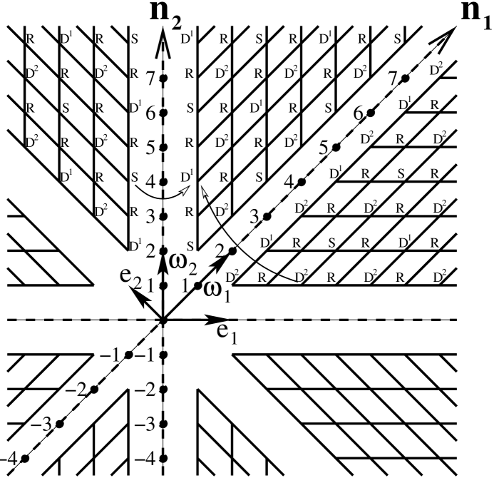
Figure 7: Kac table of the $Z_{5}$ theory, based on the weight lattice of $B_{2}$. The lattice is spanned by (one half of) the fundamental weights $\vec{\omega}_{1}$, $\vec{\omega}_{2}$. We show here the “basic layer”, i.e., the one with $(n_{1}^{\prime},n_{2}^{\prime})=(1,1)$. Each vertex of the lattice is labeled according to the nature of the associated operator ($S$, $D^{1}$, $D^{2}$, $R$). This labeling extends periodically throughout the lattice. The simple roots, $\vec{e}_{1}$ and $\vec{e}_{2}$, act as screening operators and are associated with lattice reflections (see text). The arrows give examples of pairs of operators which are linked by such reflections. The physical part of the spectrum is restricted to the wedge limited by the $n_{1}$ and $n_{2}$ axes.

The Kac table of the theory $Z_{5}$ is shown in Fig. 7, together with the vectors $\vec{e}_{1}$, $\vec{e}_{2}$ representing the screening operators of the associated (assumed) Coulomb gas representation. The labeling of each vertex of the lattice encodes the nature of the corresponding operator: singlet ($S$), doublet 1 ($D^{1}$), doublet 2 ($D^{2}$) and disorder operator ($R$). The reasoning for the particular pattern shown in the figure will be given below.

It should be observed that the Kac table of the theory $Z_{5}$ is in fact four-dimensional, made of two-dimensional layers corresponding to the $\alpha_{+}$ and $\alpha_{-}$ parts of Eq. (3.1). This separation on the $\alpha_{+}$ and $\alpha_{-}$ parts is seen more explicitly from the following form of the Kac formula:

$$\Delta_{(n_{1},n_{2})(n^{\prime}_{1},n^{\prime}_{2})}=\left[\left(\frac{n_{1}}{2}\vec{\omega}_{1}+\frac{n_{2}}{2}\vec{\omega}_{2}\right)\alpha_{+}+\left(\frac{n^{\prime}_{1}}{2}\vec{\omega}_{1}+\frac{n^{\prime}_{2}}{2}\vec{\omega}_{2}\right)\alpha_{-}\right]^{2}-\vec{\alpha}^{2}_{0}+B.$$ (4.1)

In Fig. 7 only one layer is displayed, namely the one with either $(n_{1}^{\prime},n_{2}^{\prime})=(1,1)$ or $(n_{1},n_{2})=(1,1)$. We shall refer to the layers $(n_{1},n_{2})(1,1)$ or $(1,1)(n^{\prime}_{1},n^{\prime}_{2})$ as the “basic layer” of the Kac table, corresponding to either the $\alpha_{+}$ or the $\alpha_{-}$ part of the spectrum. Such a layer is basic in the sense that the other side has trivial indices.

Also shown on Fig. 7 are examples of reflections, marked by arrows pointing from the domains on the left and on the right into the physical domain, which is the upper-right corner of the table (the wedge limited by the $n_{1}$ and $n_{2}$ axes). Just like in Felder’s resolution for minimal (Virasoro algebra) models [8], these reflections, realised by integrated screenings, indicate singular states (degeneracies) in the modules of physical operators. In this sense the operators in the adjacent domains are all “ghosts”, which decouple from the physical operators in the operator algebra, and in correlation functions. As usual, for the above reasoning based on reflections to be justified, we must assume that the screenings commute with the parafermionic algebra.

We can check these assumptions by looking at the low-lying operators in the basic layer of the Kac table, cf. Fig. 7. For the first operators of each type—$R$ (disorder), $D^{2}$ (doublet 2), $D^{1}$ (doublet 1) and $S$ (singlet)—the levels of degeneracy have been defined in Section 2 by direct calculation. Alternatively, the levels of degeneracy could be found, if our assumptions are correct, by taking the difference of the dimensions $\Delta_{(n_{1},n_{2})(n^{\prime}_{1},n^{\prime}_{2})}$, as given by Eq. (3), for two operators at the ends of the arrow representing a particular reflection in Fig. 7.

For the operator $R$, positioned as $\Phi_{(1,2)(1,1)}$ or $\Phi_{(1,1)(1,2)}$, both reflections gives the result $1/2$ for the difference of the dimensions:

$$\Delta_{(1,1)(-1,4)}-\Delta_{(1,1)(1,2)} = \frac{1}{2},$$ (4.2)

$$\Delta_{(1,1)(3,-2)}-\Delta_{(1,1)(1,2)} = \frac{1}{2}.$$ (4.3)

This agrees with the finding of Section 2 that these disorder operators are doubly degenerate at level $1/2$.

Next, for the operator $D^{1}$, at the location $\Phi_{(1,1)(1,3)}$, one finds

$$\Delta_{(1,1)(-1,5)}-\Delta_{(1,1)(1,3)} = \frac{2}{5},$$ (4.4)

$$\Delta_{(1,1)(4,-3)}-\Delta_{(1,1)(1,3)} = \frac{4}{5},$$ (4.5)

according to Fig. 7. This is in agreement with the fact that this operator is degenerate at levels $2/5$ and $4/5$, as we have found in Section 2.

In a similar way, the two reflections for the operator $D^{2}$, located as $\Phi_{(1,1)(2,1)}$, confirm the degeneracy at levels $1/5$ and $1$, as found in Section 2. And finally, in the case of the identity operator $\Phi_{(1,1)(1,1)}=I$, which is of the $S$ type, the two reflections in Fig. 7 give the differences of dimensions $2/5$ and $3/5$, in accordance with the levels of degeneracy in the identity operator module as dressed in Section 2.

It is important to note that the labeling of the ghost operator, as being $R$, $S$, $D^{1}$ or $D^{2}$ for every reflection, has to be in accordance with the nature of the corresponding state in the module of the physical operator into which the ghost operator is mapped. For instance, in the module of a $D^{1}$ operator, cf. Fig. 5, a degenerate state at level $2/5$ is a singlet, because that level belongs to the charge sector $q=0$. Likewise, a doublet of degenerate states at level $4/5$ (charge sector $q=\pm 2$) corresponds to a doublet 2 operator. Evidently, the differences of dimensions, as found in Eqs. (4.2)–(4.5), are to be calculated with the appropriate boundary terms [identified in Eq. (3.10)] in the Kac formula for $\Delta_{(n_{1},n_{2})(n^{\prime}_{1}n^{\prime}_{2})}$, cf. Eq. (3).

The disorder operators have to map among themselves, assuming that the screening operators which realise the mappings (reflections) do not translate order to disorder.

So far we have identified the nature of the following operators, situated at the low-lying corner of the physical domain shown in the table of Fig. 7:

$$\Phi_{(1,1)(1,1)} = S=I,$$ (4.6)

$$\Phi_{(1,1)(2,1)} = D^{2},$$ (4.7)

$$\Phi_{(1,1)(1,2)} = R,$$ (4.8)

$$\Phi_{(1,1)(1,3)} = D^{1}.$$ (4.9)

Similar identifications apply on the side of $\alpha_{+}$, e.g., $\Phi_{(2,1)(1,1)}=D^{2}$ etc. We now show how to fill in the rest of the basic layer, on the $\alpha_{-}$ side for instance, by making use of simple fusion rules and reflections.

We first consider the operator product

$$R\cdot D^{1}=\Phi_{(1,1)(1,2)}\cdot\Phi_{(1,1)(1,3)}.$$ (4.10)

On the left-hand side, the result of the multiplication should be a disorder operator.

On the right-hand side, according to the Coulomb gas rules, the above multiplication produces an operator, in the principal channel, with

$$\vec{\beta}_{(1,1)(1,4)}=\vec{\beta}_{(1,1)(1,2)}+\vec{\beta}_{(1,1)(1,3)}.$$ (4.11)

Multiplication of operators corresponds to addition of the corresponding vectors $\vec{\beta}$ in Fig. 7. The non-principal channels follow the principal one by shifts realised by the vectors $-\vec{e}_{1}$ and $-\vec{e}_{2}$. But for the present purposes it will be sufficient to follow the principal channel only.

At this point we should remark on a sign convention concerning the orientation of the vectors in the Coulomb gas representation. According to Eq. (3.2), the vectors $\vec{\beta}$ have a negative projection along the fundamental weight vectors $\vec{\omega}_{1}$ and $\vec{\omega}_{2}$. The usual convention in the Colomb gas representation analysis is to change their sign, i.e., to orient them positively, as seen on Fig. 7. To compensate for this convention, the moves associated with the screenings should then be realised by shifts in the direction opposite to that of the simple roots, i.e., in the direction of the vectors $-\vec{e}_{1}$ and $-\vec{e}_{2}$. Without this convention for the inversion of directions, in the graphical representation of Fig. 7, the Kac table should have been spanned by the vectors $-\vec{\omega}_{1}/2$ and $-\vec{\omega}_{2}/2$, according to Eq. (3.2). With this convention in mind, the graphical addition [with respect to the origin $(1,1)(1,1)$] of the lattice vectors in Fig. 7, corresponding to the operators $\Phi_{(1,1)(1,2)}$ and $\Phi_{(1,1)(1,3)}$ in Eq. (4.10), is in accordance with the additions of the vectors $\vec{\beta}$ in Eq. (4.11).

As a result, Eq. (4.10) leads us to conclude that the site $(1,1)(1,4)$ of the Kac table is occupied by an operator of type $R$ (disorder).

Next, we consider multiplying the operator $D^{1}=\Phi_{(1,1)(1,3)}$ with itself:

$$D^{1}\cdot D^{1}=\Phi_{(1,1)(1,3)}\cdot\Phi_{(1,1)(1,3)}.$$ (4.12)

The right-hand side produces, in the principal channel, the operator $\Phi_{(1,1)(1,5)}$. According to the left-hand side, this operator has to be either of the $D^{2}$ or the $S$ type. The result $D^{2}$ is obtained if both $D^{1}$ operators of the left-hand side of Eq. (4.12) belong to the $q=+1$ part of the doublet (or if both have $q=-1$). However, if the $Z_{5}$ charge of the two $D^{1}$ operators are opposite (one being $q=+1$ and the other $q=-1$), the left-hand side produces a singlet ($S$) operator.

This ambiguity is due to the fact that the site in the Kac table labeled $D^{1}$ is in fact the position of both members of the doublet 1, viz. operators with $q=\pm 1$. A similar remark applies to the case when a $D^{2}$ operator participates in an operator product. A site in the Kac table labeled $R$ accommodates the whole quintuplet $\{R_{a},a=1,...,5\}$ of disorder operators, all sharing a particular value of the conformal dimension $\Delta$.

The ambiguity for assigning the correct label to the operator $\Phi_{(1,1)(1,5)}$ is resolved by adding an argument based on reflections. In fact, one can check that the horizontal reflection in Fig. 7—from the ghost site on the left, across the $n_{2}$ axis, and to the site $(1,1)(1,5)$ on the right—has a “bare gap” of

$$\Delta^{(0)}_{(1,1)(-1,7)}-\Delta^{(0)}_{(1,1)(1,5)}=\frac{1}{2}.$$ (4.13)

(Here, we have defined the “bare” dimensions as $\Delta_{(n_{1},n_{2})(n_{1}^{\prime},n_{2}^{\prime})}-B$, i.e., by Eq. (3) with the boundary term being neglected.)

Suppose first that $\Phi_{(1,1)(1,5)}$ is a $D^{2}$, so that we shall have to correct the second term in Eq. (4.13) by the boundary term $B_{D^{2}}=3/20$. One now examines in turn the three possible assignments ($D^{1},D^{2}$ or $S$) of a label for the ghost site at $(1,1)(-1,7)$, each time correcting the first term in Eq. (4.13) by the corresponding boundary term. In case of a consistent assignment, the right-hand side must equal a level on which a ghost operator of the given nature can be a submodule of the physical $D^{2}$ operator. According to Fig. 6, these levels can be: $1/5+$integer if the ghost is a $D^{1}$, $3/5+$integer if it is a $S$, and $1+$integer if it is a $D^{2}$. It is easily verified that none of the three possible assignments leads to a consistent result. Therefore, $\Phi_{(1,1)(1,5)}$ cannot be a $D^{2}$ operator.

On the other hand, if $\Phi_{(1,1)(1,5)}$ is a singlet, and the calculation of the gap in Eq. (4.13) is corrected by assuming a (ghost) operator of type $D^{1}$ at the site $(1,1)(-1,7)$, then the corrected gap in Eq. (4.13) will give $3/5$. It is seen from Fig. 4 that a singlet operator can indeed accommodate a $D^{1}$ submodule at level $3/5$. Moreover, $D^{1}$ is the only consistent labeling of the ghost operator.

The result of the above series of arguments is that the operator $\Phi_{(1,1)(1,5)}$ is a singlet (and also that the ghost operator $\Phi_{(1,1)(-1,7)}$ is a doublet 1).

At the other border of the physical domain, which is parallel to the $n_{1}$ axis, by using a similar series of arguments one concludes that the operator $\Phi_{(1,1)(3,1)}$, situated next to $D^{2}=\Phi_{(1,1)(2,1)}$, can only be a singlet. More precisely, in this case the bare gap for the reflection across the $n_{1}$ axis reads:

$$\Delta^{(0)}_{(1,1)(4,-1)}-\Delta^{(0)}_{(1,1)(3,1)}=\frac{1}{4}$$ (4.14)

By correcting this formula by boundary terms, it can be checked that the only labels that can be consistently assigned to the sites $(1,1)(4,-1)$ and $(1,1)(3,1)$ are those given in Fig. 7.

Having defined the positions of the first nontrivial singlets, i.e., the operators $\Phi_{(1,1)(3,1)}$ and $\Phi_{(1,1)(1,5)}$, we can now extend the singlets over the whole lattice (the basic layer in Fig. 7). To this end, it suffices to multiply the singlets among themselves. In the products they produce only singlets, and we shall cover the lattice by adding the corresponding lattice vectors. Put differently, the lattice vectors corresponding to the operators $\Phi_{(1,1)(3,1)}$ and $\Phi_{(1,1)(1,5)}$ are the fundamental ones for the sublattice of singlet operators.

Next, we can extend the labeling $D^{2}$ of the site $(1,1)(2,1)$ out over the entire lattice. This is done by multiplying $\Phi_{(1,1)(2,1)}$ by all possible singlets. As the singlet consists of only one $q=0$ state, the argument based on addition of $Z_{5}$ charges involves no ambiguity, and the result can only be another $D^{2}$ operator. As a consequence, every fourth row parallel to the $n_{1}$ axis (viz., the rows $1,5,9,\ldots$) become completely filled out by an alternation of $S$ and $D^{2}$ operators; see Fig. 7.

It is equally easy to extend the positions of disorder operators over the whole lattice.

First, multiplying the operator $D^{1}=\Phi_{(1,1)(1,3)}$ by the basic disorder operator $R=\Phi_{(1,1)(1,2)}$ we see that $\Phi_{(1,1)(1,4)}$ must be another disorder operator. Furthermore, the operators $\Phi_{(1,1),(2,2)}$ and $\Phi_{(1,1),(2,4)}$ are also disorder operators. This is seen by multiplying the first two disorder operators, $\Phi_{(1,1)(1,2)}$ and $\Phi_{(1,1)(1,4)}$, by the basic doublet, $D^{2}=\Phi_{(1,1)(2,1)}$.

Second, the above four disorder operators can be extended throughout the lattice by multiplying them by all possible singlets. In all cases, the result must be a disorder operator. We conclude that every second row of the physical domain is occupied exclusively by disorder operators, as shown on Fig. 7.

At this point, only the rows $3,7,11,\ldots$ in the basic layer remain to be determined. In fact, once the nature of the operators $\Phi_{(1,1)(1,3)}$ and $\Phi_{(1,1),(2,3)}$ is determined, these two operators can be extended throughout the entire lattice by repeated multiplication by the two fundamental singlets, at positions $(1,1)(3,1)$ and $(1,1)(1,5)$. The result will be that the rows in question will realise an alternating sequence of these two operators.

The operator $\Phi_{(1,1)(1,3)}$ is, of course, already known: it is the fundamental doublet 1 ($D^{1}$). It remains to define $\Phi_{(1,1),(2,3)}$. Actually, by assuming the whole lattice—and not just the physical domain—to be filled out in a homogeneous (periodic) way, we could equivalently ask for the labeling of $\Phi_{(1,1)(2,-1)}$, four rows below. Now, by consistency of reflections with the levels in the module of the identity operator $S=I=\Phi_{(1,1)(1,1)}$, the ghost operator $\Phi_{(1,1)(2,-1)}$ has to be $D^{2}$. It is easy to check that this accounts for the degeneracy at level 2/5. The identification of $\Phi_{(1,1)(2,3)}$ as a doublet 2 operator is also confirmed by a direct degeneracy calculations given in Appendix D.

We thus reach the conclusion that the rows $3,7,11,\ldots$ in the basic layer are occupied by an alternation of $D^{1}$ and $D^{2}$ operators, as shown on Fig. 7.

Conclusion: By a series of arguments described above, where we have combined reflections and simple fusion rules, we have filled the whole lattice corresponding to the basic layer. The result is shown in Fig. 7.

The sites in the other layers, in which the indices of $\Delta_{(n_{1},n_{2})(n^{\prime}_{1}n^{\prime}_{2})}$ are nontrivial on both the $\alpha_{+}$ and the $\alpha_{-}$ sides, must also be assigned $S$, $D^{1}$, $D^{2}$ and $R$ labels. We now show how this can be accomplished by shifting the labels assigned to the basic layer.

Figure 8: Assingment of labels to the operators in the layer $\Phi_{(1,2)(n^{\prime}_{1},n^{\prime}_{2})}$. This is obtained by shifting the labels of Fig. 7.

Let us assume, for definiteness, that the lattice in Fig. 7 corresponds to the operators on the $\alpha_{-}$ side, i.e., the operators $\Phi_{(1,1)(n^{\prime}_{1},n^{\prime}_{2})}$ whose indices on the $\alpha_{+}$ side are trivial, $n_{1}=n_{2}=1$. Now consider, for instance, the operators $\Phi_{(1,2)(n^{\prime}_{1},n^{\prime}_{2})}$ having the “excitation” $(1,2)$ on the $\alpha_{+}$ side. In this case the assignment of $S$, $D^{1}$, $D^{2}$ and $R$ labels to the corresponding two-dimensional lattice with coordinates $(n^{\prime}_{1},n^{\prime}_{2})$ is simply obtained by a shift of the distribution of $S$, $D^{1}$, $D^{2}$ and $R$ in the basic layer (see Fig. 7) along the vector $(1,2)$. The result is shown in Fig. 8.

Put otherwise, the label of a generic operator $\Phi_{(n_{1},n_{2})(n_{1}^{\prime},n_{2}^{\prime})}$ only depends on the differences of indices, $(n_{1}-n_{1}^{\prime},n_{2}-n_{2}^{\prime})$. Therefore, the label of $\Phi_{(n_{1},n_{2})(n_{1}^{\prime},n_{2}^{\prime})}$ coincides with that of $\Phi_{(1,1),(n_{1}^{\prime}+1-n_{1},n_{2}^{\prime}+1-n_{2})}$. As this latter operator belongs to the basic layer, depicted in Fig. 7, the corresponding label is known.

We remark that the above shifting argument could just as well have been used to trivialise the indices on the $\alpha_{-}$ side. Thus, the label of $\Phi_{(n_{1},n_{2})(n_{1}^{\prime},n_{2}^{\prime})}$ not only coincides with that of $\Phi_{(1,1),(n_{1}^{\prime}+1-n_{1},n_{2}^{\prime}+1-n_{2})}$ but also with that of $\Phi_{(n_{1}+1-n_{1}^{\prime},n_{2}+1-n_{2}^{\prime})(1,1)}$. Both these latter operators belong to the basic layer, since the distinction between the $\alpha_{+}$ and $\alpha_{-}$ sides is just a convention. We can therefore conclude that the labels of $\Phi_{(1,1),(1+\tilde{n}_{1},1+\tilde{n}_{2})}$ and $\Phi_{(1,1),(1-\tilde{n}_{1},1-\tilde{n}_{2})}$ coincide, for any integers $\tilde{n}_{1}$ and $\tilde{n}_{2}$.

The presentation described above—and in particular the notions of “basic layer” and “other layers”—is of course just one particular way which we have chosen to visualise the four-dimensional lattice of operators $\Phi_{(n_{1},n_{2})(n^{\prime}_{1},n^{\prime}_{2})}$.

4.2 Finite Kac tables for unitary theories

All the discussion so far on the Kac table applies in general, when the parameters $\alpha_{+}$ and $\alpha_{-}=-1/\alpha_{+}$ take general values. As usual, when $\alpha^{2}_{+}$ takes rational values, the Kac table becomes finite. For unitary theories $\alpha^{2}_{+}=(p+2)/p$, cf. Eqs. (2.62) and (3.3), with $p$ being an integer. The physical operators’ part of the Kac table will then be delimited by:

$$2\leq n^{\prime}_{1}+n^{\prime}_{2}\leq p+1,$$

$$2\leq n_{1}+n_{2}\leq p-1.$$ (4.15)

This is similar to the Kac table of the conformal theory $WB_{2}$, defined, among other $W$ theories, by Fateev and Lukyanov in Ref. [9]. The contents of this conformal theory ($WB_{2}$) and the one considered in the present paper ($Z_{5}$, second solution) are completely different. Still, both of them use the weight lattice of the algebra $B_{2}$ for their respective representations. And the global properties of their representation lattices (the Kac tables) are the same.

The delimitations of the Kac table of the theory $Z_{5}$, as given in Eq. (4.15), can also be checked directly. To this end, we consider reflections in the direction

$$2\vec{e}_{2}+\vec{e}_{1}.$$ (4.16)

Using Eq. (3) for $\Delta_{(n_{1},n_{2})(n^{\prime}_{1},n^{\prime}_{2})}$, together with the appropriate boundary terms established above, one finds that the operators above the line

$$n^{\prime}_{1}+n^{\prime}_{2}=p+2$$ (4.17)

in Fig. 7 are all ghosts, which should decouple. Their dimensions differ from those of their partners with respect to the reflections in the line (4.17) by values which are consistent with the levels in the corresponding modules. These reflections are realised by screenings that are units of the vector (4.16) [which is itself made out of three screenings]. This is sufficient to decouple the operators above the line (4.17).

In giving this argument, we have referred to Fig. 7, which is the basic layer of the Kac table. But the argument is true for the other layers as well.

Finally, the remaining finite part of the Kac table, delimited by the conditions in Eq. (4.15), possesses a further symmetry. Using Eq. (3) together with appropriate boundary terms, one can check that the operation

$$\left\{\begin{array}[]{ll}n^{\prime}_{1}\rightarrow p+2-n^{\prime}_{1}-n^{\prime}_{2},&n^{\prime}_{2}\rightarrow n^{\prime}_{2},\\ n_{1}\rightarrow p-n_{1}-n_{2},&n_{2}\rightarrow n_{2},\end{array}\right.$$ (4.20)

is a symmetry of $\Delta_{(n_{1},n_{2})(n^{\prime}_{1},n^{\prime}_{2})}$.

It is also a symmetry of the Kac table of $WB_{2}$ [9]. The basic difference of the theory $Z_{5}$, from a very general point of view, resides in its boundary terms for the different sectors. The important point is that the symmetry (4.20), as well as the decoupling of the operators outside of the domain (4.15), remains unbroken by the $S$, $D^{1}$, $D^{2}$, $R$ structure of the lattice. Rather, it is consistent with it.

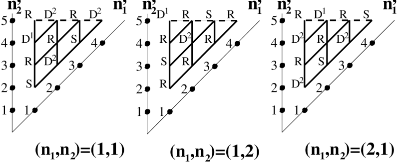
Figure 9: Kac table of the the $p=4$ theory with $c=3/2$. There are three $\alpha_{-}$ layers, having a triangular shape, and each corresponding to fixed values of the $\alpha_{+}$ indices $(n_{1},n_{2})$. In the $(1,2)$ layer, the symmetry (4.20) acts by reflecting the operators in a line that goes through the right angle of the triangle and the mid-point of the long side. In the $(1,1)$ and $(2,1)$ layers, the symmetry (4.20) acts by permuting these two layers and reflecting the triangle. The theory thus has a total of 16 primary operators.

Let us give a simple example of the series of theories that we have constructed. According to the coset formula in Eqs. (1.1)–(1.3), the first non-trivial $Z_{5}$ theory should be that with $p=p_{\rm min}=4$, having $c=3/2$. Its Kac table, which is made of three $\alpha_{-}$ layers, is shown in Fig. 9.

The preceding theory, the one with $p=3$, is trivial. Its Kac table is made of just one $\alpha_{-}$ layer, with all the operators being present $(S,R,D^{1},D^{2})$ having the trivial scaling dimension, $\Delta=0$. This could have been anticipated, because the central charge of this theory is $c=0$, according to Eq. (1.2).

4.3 Characteristic equations

In all the arguments so far, in building the Kac formula and the Kac table, we have used arguments based on the Coulomb gas. Its existance has been assumed, with given properties; we have however not constructed the Coulomb gas explicitly.

Our assumptions (in particular for the fusion rules) could be supported, at least partially, by giving characteristic equations for conformal dimensions of operators participating in a given fusion (operator algebra expansion). These can be obtained from differential equations for three-point correlation functions.

The differential equations, which are due to the degeneracy of the modules, can be derived in a way analogous to that of Ref. [6], dealing with the $Z_{3}$ theory. Below we give several examples of correlation functions and the resulting characteristic equations for the dimensions of the operators. However, we do not intend to dress an exhaustive list of such equations. Rather, the examples discussed should be considered as an additional demonstration on the consistency of our approach, and of the theory.

In Appendix C the correlation function

$$\left\langle R^{(2)}(z_{2})\Phi^{q}(z_{3})R^{(1)}(z_{1})\right\rangle$$ (4.21)

is considered. Here $R^{(1)}(z_{1})$ is a disorder operator whose module is supposed to be completely degenerate at level 1/2, i.e., $R^{(1)}(z_{1})=\Phi_{(1,2)(1,1)}(z_{1})$ or $\Phi_{(1,1)(1,2)}(z_{1})$. By $R^{(2)}(z_{2})$ we denote another, generic disorder operator, and $\Phi^{q}(z_{3})$ with $q=0,\pm 1$ is a singlet or a doublet 1 operator. For the reasons given in Appendix C, the correlation functions with a doublet 2 operator will be considered separately.

Using a method slightly different from that in Ref. [6], we have derived a differential equation for the function (4.21); see Appendix C. Here we are concerned only with the characteristic equation for dimensions which results from it. One finds that the necessary condition for the function (4.21) to be non-zero is given by the following equation on the dimensions of the operators $R^{(1)}$, $R^{(2)}$ and $\Phi^{q}$:

$$\Delta_{R^{(2)}}-\Delta_{\Phi^{q}}+\frac{1}{4}\left(1-\frac{2q^{2}}{5}\right)\Delta_{R^{(1)}}=(-1)^{q}\frac{5}{4}\frac{h^{(2)}_{1}}{h^{(1)}_{1}}\Delta_{R^{(1)}}.$$ (4.22)

Here, $h^{(1)}_{1},\,h^{(2)}_{1}$ are the zero mode eigenvalues of the operators $R^{(1)}$ and $R^{(2)}$ as defined in Eq. (2.101).

In a similar way one derives analogous results for the functions given below; see Appendix C.

• $\left\langle\Phi^{2}_{(2)}\Phi^{0}\Phi^{-2}_{(1)}\right\rangle$. The module of the operator $\Phi^{-2}_{(1)}$ is supposed to be degenerate on levels 1/5 and 1, i.e., $\Phi^{-2}_{(1)}=\Phi_{(2,1)(1,1)}$ or $\Phi_{(1,1)(2,1)}$. Using these degeneracies one derives a differential equation, from which the following equation for the dimensions:

  $$\Delta_{\Phi^{0}}-\Delta_{\Phi^{2}_{(2)}}-\frac{1}{4}\Delta_{\Phi^{2}_{(1)}}=-\frac{5}{4}\frac{h^{(2)}_{1,2}}{h^{(1)}_{1,2}}\Delta_{\Phi^{2}_{(1)}}$$ (4.23)

  is deduced. Here, $h^{(2)}_{1,2}$ and $h^{(1)}_{1,2}$ are the eigenvalues of the operators $\Phi^{2}_{(2)}$ and $\Phi^{-2}_{(1)}$ with respect to the zero modes $A^{1}_{0},A^{-1}_{0}$, as defined in Eq. (2.24).

• $\left\langle\Phi^{2}_{(2)}\Phi^{1}\Phi^{2}_{(1)}\right\rangle.$ The module of the operator $\Phi^{2}_{(1)}$ is assumed to be degenerate on levels 1/5 and 1, i.e., $\Phi^{2}_{(1)}=\Phi_{(2,1)(1,1)}$ or $\Phi_{(1,1)(2,1)}$. The operator $\Phi^{2}_{(2)}$ is more general, since in this case we assume it to be degenerate once on level 1/5, whilst its second level of degeneracy can be general. From reflection arguments it is checked that an operator with such properties can be any one in the series:

  $$\Phi^{2}_{(2)}=\Phi_{(2k,1)(1,1)}\mbox{ or }\Phi_{(1,1)(2k,1)},$$ (4.24)

  with $k=1,2,3,\ldots$. In this case the correlation function $\left\langle\Phi^{2}_{(2)}\Phi^{1}\Phi^{2}_{(1)}\right\rangle$ leads to the following characteristic equation:

  $$\Delta_{\Phi^{1}}=\Delta_{\Phi^{2}_{(2)}}+\frac{1}{2}\Delta_{\Phi^{2}_{(1)}}.$$ (4.25)

• $\left\langle\Phi^{1}_{(3)}\Phi^{1}_{(2)}\Phi^{-2}_{(1)}\right\rangle.$ Similarly, the module of the operator $\Phi^{-2}_{(1)}$ is assumed to be degenerate at levels 1/5 and 1. The operators $\Phi^{1}_{(3)}$ and $\Phi^{1}_{(2)}$ are general. The characteristic equation for this function turns ont to be very simple. This function is non-zero if:

  $$\Delta_{\Phi^{1}_{(2)}}=\Delta_{\Phi^{1}_{(3)}}.$$ (4.26)

By analysing the characteristic equations given above it is verified that they are in agreement with the general arguments based on the Coulomb gas, i.e., the arguments that we have used in defining the $S$, $D^{1}$, $D^{2}$, $R$ structure of the Kac table. They also contain some more concrete information on the fusion rules of the theory. This is the case of Eqs. (4.25) and (4.26). For instance, solving Eq. (4.25), one finds that the fusion of the operators:

$$\Phi^{2}_{(1)}=\Phi_{(1,1)(2,1)}\mbox{ and }\Phi^{2}_{(2)}=\Phi_{(1,1)(2k,1)}$$ (4.27)

produces, in particular, the operator

$$\Phi^{1}=\Phi_{(1,1)(2k-1,3)}.$$ (4.28)

This result is in agreement with the positioning of doublet 1 operators in the third row in Fig. 7. It is also in accordance with the addition of vectors, corresponding to operators in the Coulomb gas picture, and with the action of screenings. A move by $-\vec{e}_{1}$, produced by the screening $\vec{e}_{1}$, will have to be used, since the channel considered is not the principal one for the Coulomb gas fusions.

The other two equations, (4.22) and (4.23), are of a somewhat more general nature. Apart from the dimensions of the operators, these equations also involve the zero mode eigenvalues of the operators: $h^{(1)}_{1}$ and $h^{(2)}_{1}$ in Eq. (4.22), as well as $h^{(1)}_{1,2}$ and $h^{(2)}_{1,2}$ in Eq. (4.23).

The zero mode eigenvalues ($h_{1},h_{2,1},h_{1,2}$) characterise the primary operators, and the corresponding representations, of the parafermionic algebra on the same footing as the $\Delta$, which are just the eigenvalues of the Virasoro zero mode $L_{0}$. In particular, the theory possesses examples of a couple of primary operators of the same nature, disorder operators for instance, having the same values of $\Delta$ but different values of $h_{1}$. Such operators have to be considered as being different.

Such examples were also present in the $Z_{3}$ theory of Fateev-Zamolodchikov [6], in which the degeneracies on the level of $\Delta$ are lifted by different values of $h_{1}$, in particular in the disorder sector.

The presence of $h_{1}$ in Eq. (4.22), and of $h_{1,2}$ in Eq. (4.23), complicates somewhat the analysis of the corresponding fusion rules.

For some particular disorder or doublet operators, the correspondent value $h_{1}$ or $h_{1,2}$ is known. This is the case for $h^{(1)}_{1}$ of the operator $R^{(1)}$, in the correlation function $\left\langle R^{(2)}\Phi^{q}R^{(1)}\right\rangle$. Also, $h^{(1)}_{1,2}$ of the operator $\Phi^{2}_{(1)}$, in the other correlation functions, is known from the degeneracy problem at level 1/5, cf. Eq. (2.71).

In the case of the function $\left\langle R^{(2)}\Phi^{q}R^{(1)}\right\rangle$ there are two independent channels, $q=0$ and $q=1$, to be considered in Eq. (4.22). If we set $R^{(2)}=\Phi_{(1,2)(1,1)}$ or $R^{(2)}=\Phi_{(1,1)(1,2)}$, all the $h_{1}$ in Eq. (4.22) are known and the dimension $\Delta_{\Phi^{q}}$ can be easily calculated for each of the two channels.

Figure 10: The subdominant channel in the operator product $\Phi_{(1,2)(1,1)}\cdot\Phi_{(1,2)(1,1)}$ is obtained by action on the principal channel $\vec{\beta}_{(1,3)(1,1)}$ with the screenings $-\vec{e}_{1}-2\vec{e}_{2}$.

We then consider the functions:

• $\left\langle\Phi_{(1,2)(1,1)}\Phi^{q}\Phi_{(1,2)(1,1)}\right\rangle$. For the $q=0$ channel it follows from Eq. (4.22) that

  $$\Delta_{\Phi^{0}}=0.$$ (4.29)

  This result was to be expected, as the two point function $\left\langle\Phi_{(1,2)(1,1)}\Phi_{(1,2)(1,1)}\right\rangle$ is non-vanishing. More interesting is the $q=1$ channel for which Eq. (4.22) gives

  $$\Delta_{\Phi^{1}}=\Delta_{\Phi_{(1,3)(1,1)}}.$$ (4.30)

  This result is in agreement with the fact that $\Phi_{(1,3)(1,1)}$ was deduced to be a doublet 1 ($q=1$), and with the Coulomb gas rules. Indeed, as previously discussed, we expect that the multiplication $\Phi_{(1,2)(1,1)}\cdot\Phi_{(1,2)(1,1)}$ produces in the principal channel the operator with $\vec{\beta}_{(1,3)(1,1)}=\vec{\beta}_{(1,2)(1,1)}+\vec{\beta}_{(1,2)(1,1)}$; the $q=0$ channel follows the principal one by the shift $-\vec{e}_{1}-2\vec{e}_{2}$, as shown in Fig. 10.

• $\left\langle\Phi_{(1,1)(1,2)}\Phi^{q}\Phi_{(1,2)(1,1)}\right\rangle$. The associated characteristic equation for the two channels is solved by:

  $$\Delta_{\Phi^{0}} = \Delta_{\Phi_{(1,2)(1,2)}},$$

  $$\Delta_{\Phi^{1}} = \Delta_{\Phi_{(0,2)(1,2)}}.$$ (4.31)

  Once again the correctness of the labeling of the lattice and of the Coulomb gas rules is confirmed.

It is interesting to notice that the operator $\Phi_{(0,2)(1,2)}$ is not a physical one and, although decoupled from the theory, it is admitted by Eq. (4.22). This follows from the fact that the characteristic equation does not give any information about the structure constants of the operator algebra; in particular, these can be equal to zero. In the case under consideration the correlation function $\left\langle\Phi_{(1,1)(1,2)}\Phi_{(0,2)(1,2)}\Phi_{(1,2)(1,1)}\right\rangle$ is expected to vanish.

4.4 General formula for the zero mode eigenvalues of disorder operators

In contrast to the particular cases considered above, the eigenvalues $h$ are not known in general. The task thus becomes not only to fix $\Delta$ but also $h^{(2)}_{1}$ of $R^{(2)}$ in Eq. (4.22) and $h^{(2)}_{1,2}$ of $\Phi^{2}_{(2)}$ in Eq. (4.23).

We focus in the following on Eq. (4.22). One of the two channels of this equation could be used to define $h^{(2)}_{1}$, by assuming a given value of $\Delta_{\Phi^{0}}$ for instance, chosen at a particular position in the Kac table. The other channel, with $\Phi^{1}$, in which enters the same $h^{(2)}_{1}$, could then serve to check for the presence of $\Delta_{\Phi^{1}}$ at the appropriate position in the Kac table, having the value calculated from the characteristic equation (4.22). In this way some progress could be made in filling the Kac table, independently of the Coulomb gas assumptions, partially at least.

The problem could also be turned around. We could assume the results of our analysis, based on the Coulomb gas arguments, in which we have already completely defined the Kac formula for the $\Delta$. We could then use instead the characteristic equations to dress the general formula for the eigenvalues $h$.

We have succeeded in this direction for the disorder operators. To this end, we have consider the product $R^{(1)}R^{(2)}$, where $R^{(1)}=\Phi_{(1,2)(1,1)}$ and $R^{(2)}$ is again a general disorder operator, $R^{(2)}=\Phi_{(n_{1},n_{2})(n_{1}^{\prime},n_{2}^{\prime})}$ with $n_{2}+n_{2}^{\prime}$ odd.

Figure 11: Each disorder operator $R$ is surrounded by three doublets and one singlet operator, as shown in the inset. These latter four operators can be related to non-principal channels in the operator product $R^{(1)}\cdot R$, as discussed in the text. The disorder operators $R$ come in four varieties, according to their neighbouring doublet and singlet operators. The arrow labeling each $R$ shows the relative position of the singlet operator. Alternatively, the arrows point away from the $D_{1}$ operators.

In Fig. 11 we show a layer of the Kac table with fixed $\alpha_{+}$ indices. From the figure one sees that a disorder operator $R^{(2)}$ is surrounded by four operators, at the positions: $\vec{\beta}_{(n_{1}+1,n_{2})(n_{1}^{\prime},n_{2}^{\prime})}$, $\vec{\beta}_{(n_{1}-1,n_{2})(n_{1}^{\prime},n_{2}^{\prime})}$, $\vec{\beta}_{(n_{1}-1,n_{2}+1)(n_{1}^{\prime},n_{2}^{\prime})}$ and $\vec{\beta}_{(n_{1}+1,n_{2}-1)(n_{1}^{\prime},n_{2}^{\prime})}$. Among these four nearest-neighbour operators, two are $D^{2}$ doublets, one is a $D^{1}$ doublet and one is a singlet $S$. It is straightforward to verify that (see the inset of Fig. 11):

$$\vec{\beta}_{(n_{1}+1,n_{2}-1)(n_{1}^{\prime},n_{2}^{\prime})} = \vec{\beta}_{(n_{1}+1,n_{2})(n_{1}^{\prime},n_{2}^{\prime})}-\vec{e}_{2},$$

$$\vec{\beta}_{(n_{1}-1,n_{2}+1)(n_{1}^{\prime},n_{2}^{\prime})} = \vec{\beta}_{(n_{1}+1,n_{2})(n_{1}^{\prime},n_{2}^{\prime})}-\vec{e}_{2}-\vec{e}_{1},$$

$$\vec{\beta}_{(n_{1},n_{2}-1)(n_{1}^{\prime},n_{2}^{\prime})} = \vec{\beta}_{(n_{1}+1,n_{2})(n_{1}^{\prime},n_{2}^{\prime})}-2\vec{e}_{2}-\vec{e}_{1}.$$ (4.32)

According to the Coulomb gas rules, the operator $\Phi_{(n_{1}+1,n_{2})(n_{1},n_{2}^{\prime})}$ is produced in the principal channel of the operator product expansion of $R^{(1)}\cdot R^{(2)}$ [indeed, $\vec{\beta}_{(n_{1}+1,n_{2})(n_{1}^{\prime},n_{2}^{\prime})}=\vec{\beta}_{(1,2)(1,1)}+\vec{\beta}_{(n_{1},n_{2})(n_{1}^{\prime},n_{2}^{\prime})}$], while the other three nearest-neighbour operators can be present in the non-principal channels of the above expansion.

Therefore we can make the natural hypothesis that the doublets $D^{1}$ and the singlet $S$, which are the nearest to $R^{2}$ in the layer $(n_{1}^{\prime},n_{2}^{\prime})$, are present in the operator product expansion of $R^{(1)}\cdot R^{(2)}$. As we showed previously, this hypothesis is verified in the case when $R^{(2)}$ is taken to be completely degenerate at level $1/2$.

We then assume that for $q=0$ (resp. $q=1$), $\Delta_{\Phi^{0}}$ (resp. $\Delta_{\Phi^{1}}$) is equal to the dimension of the nearest singlet $S$ (resp. doublet $D^{1}$). The eigenvalue $h^{(2)}_{1}$ can now be determined by solving the correspondent equation.

Once $h^{(2)}_{1}$ has been fixed, for example using the $q=0$ channel, one can easily check that Eq. (4.22) admits in the $q=1$ channel the nearest-neighbour doublet $D^{1}$. The above assumption is thus perfectly consistent with the characteristic equation.

We can label quite naturally a disorder operator by its relative position with respect to the nearest singlet. As shown on Fig. 11, four types of disorder operators can then be identified, namely $R_{\uparrow}$, $R_{\downarrow}$, $R_{\leftarrow}$ and $R_{\rightarrow}$. The general formula for the eigenvalue $h^{X}_{1}$ of the disorder operator $\Phi_{(n_{1},n_{2})(n_{1}^{\prime},n_{2}^{\prime})}$ of type $X$ ($X=\ \uparrow,\downarrow,\leftarrow,\rightarrow$) turns out to be:

$$h^{\downarrow}_{1} = A\left[4\,(n_{1}+n_{2})\,p-4\,(n_{1}^{\prime}+n_{2}^{\prime})(p+2)+p+1\right],$$

$$h^{\uparrow}_{1} = A\left[-4\,(n_{1}+n_{2})\,p+4\,(n_{1}^{\prime}+n_{2}^{\prime})(p+2)+p+1\right],$$

$$h^{\leftarrow}_{1} = A\left[4\,n_{1}\,p-4\,n_{1}^{\prime}(p+2)+p+1\right],$$

$$h^{\rightarrow}_{1} = A\left[-4\,n_{1}\,p+4\,n_{1}^{\prime}\,(p+2)+p+1\right],$$ (4.33)

where

$$A=\frac{1}{80}\frac{\sqrt{5}\;2^{\frac{4}{5}}}{\sqrt{p-3}\,\sqrt{p+5}}.$$ (4.34)

Notice that the symmetry (4.20) of the Kac table is respected by Eq. (4.33).

The above analysis could also be done by studying the fusion $R^{(1)}\cdot R^{(2)}$ with $R^{(1)}=\Phi_{(1,1)(1,2)}$. It is easy to verify that this procedure leads to the same results.

In the following we shall give a partial verification of Eq. (4.33) by determining explicitly the eigenvalue $h_{1}$ for a subset of disorder operators.

Figure 12: The reflections shown on the figure are used to demonstrate that a subset of disorder operators belonging to the physical domain all have one degeneracy at level $1/2$. Apart from the fundamental disorder operator $\Phi_{(1,1)(1,2)}$, the other degeneracy is at a more descendent level than $1/2$.

As shown in Fig. 12, where the particular layer $(1,1)(n_{1}^{\prime},n_{2}^{\prime})$ is represented, there are two reflections, one by the vector $-\vec{e}_{1}$ and the other by the vector $-2\vec{e}_{2}$, which give the differences

$$\Delta_{(1,n_{2})(-1,n_{2}^{\prime}+2)}-\Delta_{(1,n_{2})(1,n_{2}^{\prime})} = \frac{1}{2},$$ (4.35)

$$\Delta_{(n_{1},1)(n_{1}^{\prime}+1,-1)}-\Delta_{(n_{1}^{\prime},1)(n_{1}^{\prime},1)} = \frac{1}{2},$$ (4.36)

respectively for $R=\Phi_{(1,n_{2})(1,n_{2}^{\prime})}$ (with $n_{1}^{\prime}+n_{2}^{\prime}$ even) and for $R=\Phi_{(n_{1},1)(n_{1}^{\prime},2)}$. These operators should therefore be partially degenerate at level $1/2$.

In Section 2 we required complete degeneracy at level $1/2$. If now we demand only a partial degeneracy at this level, we do have one less constraint. The eigenvalues $h_{1}$ and $h_{2}$ will be determined as functions of the dimension $\Delta_{R}$ and of the central charge. Then, if we use the value $\Delta_{R}$ provided by the Kac formula, we have finally access to the expression of $h_{1}$ and $h_{2}$ for $R=\Phi_{(1,n_{2})(1,n_{2}^{\prime})}$ (with $n_{1}^{\prime}+n_{2}^{\prime}$ odd) and for $R=\Phi_{(n_{1},1)(n_{1}^{\prime},2)}$.

At level $1/2$ of the module $R_{a}$ there are two states, namely $\left(\chi^{(1)}_{a}\right)_{-\frac{1}{2}}$ and $\left(\chi^{(2)}_{a}\right)_{-\frac{1}{2}}$, as defined in Eqs. (2.105) and (2.106). We consider the linear combination

$$\chi_{-\frac{1}{2}}=a(\chi^{(1)}_{a})_{-\frac{1}{2}}+b(\chi^{(2)}_{a})_{-\frac{1}{2}}$$ (4.37)

which would be primary. As usual, we then require that

$$A^{1}_{+\frac{1}{2}}\chi_{-\frac{1}{2}}=A^{2}_{+\frac{1}{2}}\chi_{-\frac{1}{2}}=0.$$ (4.38)

Using Eq. (4.37), one has from Eq. (4.38) that

$$aA^{1}_{\frac{1}{2}}A^{1}_{-\frac{1}{2}}R_{a}+bA^{1}_{\frac{1}{2}}A^{2}_{-\frac{1}{2}}R_{a} = 0,$$

$$aA^{2}_{\frac{1}{2}}A^{1}_{-\frac{1}{2}}R_{a}+bA^{2}_{\frac{2}{5}}A^{2}_{-\frac{2}{5}}R_{a} = 0.$$ (4.39)

Defining now $\mu^{(i,j)}$ as $A^{i}_{\frac{1}{2}}A^{j}_{-\frac{1}{2}}R_{a^{\prime}}\equiv\mu^{(i,j)}R_{a}$, the above system can be solved if

$$\mu^{(1,1)}\mu^{(2,2)}-\mu^{(1,2)}\mu^{(2,1)}=0.$$ (4.40)

The values of $\mu^{(i,j)}$ as a function of $h_{1}$, $h_{2}$ and $\Delta_{R}$ can be extracted from Eqs. (2.111), (2.113) and (2.115). Applying then Eq. (2.104), it is straightforward to see that Eq. (4.40) results in a sixth-degree equation in $h_{1}$. Setting $\Delta_{R}=\Delta_{(1,n_{2})(1,n_{2}^{\prime})}$ or $\Delta_{R}=\Delta_{(n_{1}^{\prime},1)(n_{1}^{\prime},1)}$, this equation presents six real solutions. Among these, one coincides with the value of $h_{1}$ given by Eq. (4.33).

In Section 2 we examined the degeneracies at the first descendent levels of the modules, and we found a number of solutions for the dimensions which we considered non-physical. The case under consideration is analogous: for each of the above operators, there is only one value of $h_{1}$ that fits with the theory that we have built. The other solutions are rejected as non-physical ones.

5 Discussion

In this paper we have constructed and analysed in some detail the $Z_{5}$ parafermionic conformal theory, based on the second solution for the corresponding parafermionic algebra [1].

Our principal result is the Kac table and the Kac formula of this theory, i.e., the formula for conformal dimensions of primary operators which realise degenerate representations of the parafermionic algebra. This formula is given, in different forms, by Eqs. (3.1), (3) and (4.1). Its boundary term $B$ is defined as follows:

$$\begin{array}[]{llll}\mbox{Singlet sector:}&B_{S}=0&n_{1}^{\prime}-n_{1}=0\mbox{ mod }2,&n_{2}^{\prime}-n_{2}=0\mbox{ mod }4\\ \mbox{Doublet 1 sector:}&B_{D^{1}}=\frac{1}{10}&n_{1}^{\prime}-n_{1}=0\mbox{ mod }2,&n_{2}^{\prime}-n_{2}=2\mbox{ mod }4\\ \mbox{Doublet 2 sector:}&B_{D^{2}}=\frac{3}{20}&n_{1}^{\prime}-n_{1}=1\mbox{ mod }2,&n_{2}^{\prime}-n_{2}=0\mbox{ mod }2\\ \mbox{Disorder sector:}&B_{R}=\frac{1}{8}&n_{1}^{\prime}-n_{1}=0\mbox{ mod }1,&n_{2}^{\prime}-n_{2}=1\mbox{ mod }2\\ \end{array}$$ (5.1)

Graphically, the distribution of operators belonging to different sectors is depicted in Fig. 7 in the case of the basic layer, $(1,1)(n^{\prime}_{1},n^{\prime}_{2})$. This figure actually contains the full information, since the other layers, with $(n_{1},n_{2})\neq(1,1)$, are obtained by translating the labels in the basic layer, cf. Eq. 5.1.

In analogy with the theory $Z_{3}$ [3], we find it natural to assume that the infinite set of $Z_{5}$ theories that we have defined, labeled by the parameter $p=4,5,6,\ldots$, describes higher multicritial points in statistical models with $Z_{5}$ symmetry.

Figure 13: Conformal dimensions $\Delta$ of fields in the $Z_{5}$ theory with $p=4$ and $c=3/2$, that are primary with respect to the parafermionic currents. The conventions for the $(n_{1},n_{2})(n_{1}^{\prime},n_{2}^{\prime})$ labels are as in Fig. 7.

The first and the simplest member in this set is the theory with $p=4$, having $c=\frac{3}{2}$, which we have already mentioned as an example in the previous section. The three layers of its Kac table are given in Fig. 9. The explicit values of the conformal dimensions of its 16 different primary operators are shown in Fig. 13. By primary, we here mean primary with respect to the parafermionic currents. Note that these operators are linked by the symmetry (4.20), which has been explained in graphical terms in the caption of Fig. 9.

Figure 14: Conformal dimensions of fields that are primary with respect to the Virasoro subalgebra (but descendents on the first two levels with respect to the parafermionic currents).

It should be added that the first and second descendents of the operators in Fig. 9 are still Virasoro algebra primaries. Their dimensions are obtained from those in Fig. 13 by adding:

$$\begin{array}[]{lll}\frac{2}{5}\mbox{ and }\frac{3}{5}&\mbox{for}&S,\\ \frac{2}{5}\mbox{ and }\frac{4}{5}&\mbox{for}&D^{1},\\ \frac{1}{5}\mbox{ and }\frac{3}{5}&\mbox{for}&D^{2},\\ \frac{1}{2}&\mbox{for}&R.\\ \end{array}$$ (5.2)

These numbers are is in accordance with the structure of the modules, as shown in Figs. 4–6. Explicit values for the resulting conformal dimensions are shown in Fig. 14.

One could conjecture that it should be possible to suitably modify the $Z_{N}$ symmetric lattice models defined in Refs. [1,2], which realise the first solution for $Z_{N}$ parafermionic theories, so as to drive them to multicriticality while preserving $Z_{N}$ symmetry. If so, the tricritical point corresponding to the theory $Z_{5}$, with $p=4$, would be the simplest example to be discovered.

From a theoretical point of view, another principal result of our paper is that the $B_{n}$ algebra lattices accommodate the representations of conformal theories with $Z_{N}$ symmetry. So far, those lattices were known to be relevant only for the $W$ theories $WB_{n}$ [9]. In the present paper we have given the demonstration of this result for the particular case of $B_{2}$, corresponding to the $Z_{5}$ theory.

In our next paper [4] we shall give the generalisation to $B_{n}$, with $n>2$ general, corresponding to the $Z_{N}$ theory with $N=2n+1$. This series is the second solution of the $Z_{N}$ parafermionic theory with $N$ odd. The case of $Z_{N}$ with $N$ even has to be studied separately. It has new features, not present in the theories with $N$ odd. The Kac table for these theories should be built on $D_{n}$ lattices, with $N=2n$.

Acknowledgments: We would like to thank P. Degiovanni, V. A. Fateev, and P. Mathieu for very useful discussions. We are particularly grateful to M.-A. Lewis, F. Merz, and M. Picco for their collaboration during the initial stages of this project.

Appendix A Mode operator commutation relations in the sectors of singlet, doublet 1 and doublet 2 operators

In general, the mode operators are defined by integrals of the type

$$A_{-\delta+m}\Phi(0) = \frac{1}{2\pi i}\oint{\rm d}z\,(z)^{\Delta_{\Psi}-\delta+m-1}\Psi(z)\Phi(0),$$ (A1)

$$\Psi(z)\Phi(0) = \sum_{m}\frac{1}{(z)^{\Delta_{\Psi}-\delta+m}}A_{-\delta+m}\Phi(0),$$ (A2)

where $\delta$ represents the first gap in the corresponding module. Explicit definitions for the mode operators in the various sectors have been given in Eqs. (2.17)–(2.18) for the singlet sector, in Eqs. (2.25)–(2.28) for the doublet 1, and in Eqs. (2.33)–(2.36) for the doublet 2.

The algebra of the mode operators, in the form of commutation relations, can be calculated by combining these definitions with the algebra of the chiral operators, Eqs. (2)–(2.2).

A.1 An example: Computation of $\{\Psi^{1},\Psi^{1}\}\Phi^{-1}$

In analogy with the methods used in Refs. [1,3], the commutation relation of the modes $A^{1}_{\mu}$ in the sector of $\Phi^{-1}$ can be derived from the integral:

$$I=\frac{1}{(2\pi i)^{2}}\oint_{C^{1}_{0}}{\rm d}z^{\prime}\oint_{C_{0}}{\rm d}z\,(z^{\prime})^{\Delta_{1}-\frac{2}{5}+n-1}(z)^{\Delta_{1}-\frac{2}{5}+m-1}$$

$$\times(z^{\prime}-z)^{2\Delta_{1}-\Delta_{2}-1}\Psi^{1}(z^{\prime})\Psi^{1}(z)\Phi^{-1}(0)$$ (A3)

In this integral the fractions $-2/5$ in the powers of $z^{\prime}$ and $z$ are in correspondence with the levels of the first descendents in the module of $\Phi^{-1}$; see Fig. 5. They will be the first operators, the dominant ones, in the operator product expansion of $\Psi^{1}(z^{\prime})\Phi^{-1}(0)$ and $\Psi^{1}(z)\Phi^{-1}(0)$, respectively.

Let us also comment on the presence of the factor $(z^{\prime}-z)^{2\Delta_{1}-\Delta_{2}-1}$. In general, an operator product $\Psi^{q^{\prime}}(z^{\prime})\Psi^{q}(z)$ must be accompanied by a factor of of $(z^{\prime}-z)^{\Delta_{q^{\prime}}+\Delta_{q}-\Delta_{q^{\prime}+q}}$ to compensate for the abelian monodromy of the two chiral fields, i.e., the phase factor which is produced when one of the fields, say $\Psi^{q^{\prime}}(z^{\prime})$, is analytically continued around the other one, $\Psi^{q}(z)$. To pick up the relevant terms in the operator product expansions (2)–(2.2) we shall need an additional integer shift $p$, making the total factor $(z^{\prime}-z)^{\Delta_{q^{\prime}}+\Delta_{q}-\Delta_{q^{\prime}+q}-p}$.

In order to touch all terms appearing explicitly in Eqs. (2)–(2.2) one should take $p=2$ when $q^{\prime}+q\neq 0$ and $p=3$ when $q^{\prime}+q=0$. In the latter case we pick up the stress energy operator $T(z)$ in the expansion, thus making connection with the Virasoro algebra.

There is one exception to this rule. Namely, in the case of a product of identical operators, such as $\Psi^{1}(z^{\prime})\Psi^{1}(z)$ above, keeping the derivative term $\partial\Psi^{2}(z)$ in Eq. (2) does not bring new information into the commutation relation. For this reason we shall take the shift $p=1$ when $q=q^{\prime}$.

Treating the integral (A3) in the same way as it has been done in Ref. [1,3], one obtains the commutation relation in the form of an infinite sum:

$$\sum^{\infty}_{l=0}D^{l}_{-\frac{1}{5}}[A^{1}_{-\frac{3}{5}+n-l}A^{1}_{-\frac{2}{5}+m+l}+A_{-\frac{3}{5}+m-l}^{1}A^{1}_{-\frac{2}{5}+n+l}]\Phi^{-1}(0)=\lambda^{1,1}_{2}A^{2}_{n+m-1}\Phi^{-1}(0).$$ (A4)

Here the coefficients $D^{l}_{\alpha}$ are defined by the expansion

$$(1-x)^{\alpha}=\sum^{\infty}_{l=0}D^{l}_{\alpha}x^{l},$$ (A5)

and in general $\alpha=\Delta_{k^{\prime}}+\Delta_{k}-\Delta_{k^{\prime}+k}-p$. Note that the sign between the terms on the left-hand side of the commutation relation (A4) is determined by the parity of $p$. Thus, it is plus for $p=1,3$ and minus for $p=2$.

A.2 List of commutation relations

Proceeding in a way similar to the above example, one can obtain the algebra of the various mode operators, in the various sectors of representation fields. For convenience, we give the complete list of algebras in Table 1. When referring to these relations we shall use a shorthand notation of the type $\{\Psi^{k},\Psi^{l}\}\Phi^{m}$, which is reproduced to the left of each entry in the table.

Presumably not all of the commutation relations given in Table 1 are needed for the degeneracy calculations, which gave the results presented in Section 2. But we have found that a large number of them are needed. So we have chosen to present the whole list, which grew on itself in various trials of preliminary calculations, without giving extra effort to reduce it somewhat.

Table 1: Commutation relations for the parafermionic mode operators $\Psi^{k}$, in the basis of singlet and doublet representation fields $\Phi^{m}$.

$\{\Psi^{1},\Psi^{1}\}\Phi^{-2}$	$\sum^{\infty}_{l=0}D^{l}_{-\frac{1}{5}}[A^{1}_{-\frac{2}{5}+n-l}A^{1}_{-\frac{1}{5}+m+l}+A^{1}_{-\frac{2}{5}+m-l}A^{1}_{-\frac{1}{5}+n+l}]\Phi^{-2}$	$=$	$\lambda^{1,1}_{2}A^{2}_{-\frac{3}{5}+n+m}\Phi^{-2}$
$\{\Psi^{1},\Psi^{1}\}\Phi^{-1}$	$\sum^{\infty}_{l=0}D^{l}_{-\frac{1}{5}}[A^{1}_{-\frac{3}{5}+n-l}A^{1}_{-\frac{2}{5}+m+l}+A_{-\frac{3}{5}+m-l}^{1}A^{1}_{-\frac{2}{5}+n+l}]\Phi^{-1}$	$=$	$\lambda^{1,1}_{2}A^{2}_{n+m-1}\Phi^{-1}$
$\{\Psi^{1},\Psi^{1}\}\Phi^{0}$	$\sum^{\infty}_{l=0}D^{l}_{-\frac{1}{5}}[A^{1}_{-\frac{4}{5}+n-l}A^{1}_{-\frac{3}{5}+m+l}+A^{1}_{-\frac{4}{5}+m-l}A^{1}_{-\frac{3}{5}+n+l}]\Phi^{0}$	$=$	$\lambda^{1,1}_{2}A^{2}_{-\frac{2}{5}+n+m-1}\Phi^{0}$
$\{\Psi^{1},\Psi^{1}\}\Phi^{1}$	$\sum^{\infty}_{l=0}D^{l}_{-\frac{1}{5}}[A^{1}_{n-l-1}A^{1}_{-\frac{4}{5}+m+l}+A^{1}_{m-l-1}A^{1}_{-\frac{4}{5}+n+l}]\Phi^{1}$	$=$	$\lambda^{1,1}_{2}A^{2}_{-\frac{4}{5}+n+m-1}\Phi^{1}$
$\{\Psi^{1},\Psi^{1}\}\Phi^{2}$	$\sum^{\infty}_{l=0}D^{l}_{-\frac{1}{5}}[A^{1}_{-\frac{1}{5}+n-l}A^{1}_{m+l}+A^{1}_{-\frac{1}{5}+m-l}A^{1}_{n+l}]\Phi^{2}$	$=$	$\lambda^{1,1}_{2}A^{2}_{-\frac{1}{5}+n+m}\Phi^{2}$
$\{\Psi^{1},\Psi^{-1}\}\Phi^{0}$	$\sum^{\infty}_{l=0}D^{l}_{\frac{1}{5}}[A^{1}_{-\frac{2}{5}+n-l}A^{-1}_{-\frac{3}{5}+m+l}+A^{-1}_{-\frac{2}{5}+m-l}A^{1}_{-\frac{3}{5}+n+l}]\Phi^{0}$	$=$	$\{\frac{1}{2}n(n-1)\delta_{n+m-1,0}+\frac{2\Delta_{1}}{c}L_{n+m-1}\}\Phi^{0}$
$\{\Psi^{1},\Psi^{-1}\}\Phi^{1}$	$\sum^{\infty}_{l=0}D^{l}_{\frac{1}{5}}[A^{1}_{-\frac{3}{5}+n-l}A^{-1}_{-\frac{2}{5}+m+l}+A^{-1}_{-\frac{1}{5}+m-l}A^{1}_{-\frac{4}{5}+n+l}]\Phi^{1}$	$=$	$\left\{\frac{1}{2}(n-\frac{1}{5})(n-\frac{6}{5})\delta_{n+m-1,0}+\frac{2\Delta_{1}}{c}L_{n+m-1}\right\}\Phi^{1}$
$\{\Psi^{1},\Psi^{-1}\}\Phi^{2}$	$\sum^{\infty}_{l=0}D^{l}_{\frac{1}{5}}[A^{-1}_{n-l}A^{1}_{m+l}+A^{1}_{-\frac{4}{5}+m-l+1}A^{-1}_{-\frac{1}{5}+n+l}]\Phi^{2}$	$=$	$\left\{\frac{1}{2}(n+\frac{2}{5})(n-\frac{3}{5})\delta_{n+m,0}+\frac{2\Delta_{1}}{c}L_{n+m}\right\}\Phi^{2}$
$\{\Psi^{1},\Psi^{2}\}\Phi^{-2}$	$\sum^{\infty}_{l=0}D^{l}_{-\frac{2}{5}}[A^{1}_{-\frac{3}{5}+n-l}A^{2}_{-\frac{3}{5}+m+l}-A^{2}_{m-l-1}A^{1}_{-\frac{1}{5}+n+l}]\Phi^{-2}$	$=$	$\lambda^{1,2}_{-2}\frac{2n-m}{3}A^{-2}_{-\frac{1}{5}+n+m-1}\Phi^{-2}$
$\{\Psi^{1},\Psi^{2}\}\Phi^{-1}$	$\sum^{\infty}_{l=0}D^{l}_{-\frac{2}{5}}[A^{1}_{-\frac{4}{5}+n-l}A^{2}_{m+l}-A^{2}_{-\frac{2}{5}+m-l}A^{1}_{-\frac{2}{5}+n+l}]\Phi^{-1}$	$=$	$\lambda_{-2}^{1,2}\frac{2n-m-1}{3}A^{-2}_{-\frac{4}{5}+n+m}\Phi^{-1}$
$\{\Psi^{1},\Psi^{2}\}\Phi^{0}$	$\sum^{\infty}_{l=0}D^{l}_{-\frac{2}{5}}[A^{2}_{-\frac{4}{5}+n-l}A^{1}_{-\frac{3}{5}+m+l}-A^{1}_{m-l-1}A^{2}_{-\frac{2}{5}+n+l}]\Phi^{0}$	$=$	$\lambda_{-2}^{1,2}\frac{n-2m+1}{3}A^{-2}_{-\frac{2}{5}+n+m-1}\Phi^{0}$
$\{\Psi^{1},\Psi^{2}\}\Phi^{1}$	$\sum^{\infty}_{l=0}D^{l}_{-\frac{2}{5}}[A^{2}_{-\frac{1}{5}+n-l-1}A^{1}_{-\frac{4}{5}+m+l}-A^{1}_{-\frac{1}{5}+m-l-1}A^{2}_{-\frac{4}{5}+n+l}]\Phi^{1}$	$=$	$\lambda_{-2}^{1,2}\frac{n-2m+1}{3}A^{-2}_{n+m-2}\Phi^{1}$
$\{\Psi^{1},\Psi^{2}\}\Phi^{2}$	$\sum^{\infty}_{l=0}D^{l}_{-\frac{2}{5}}[A^{1}_{-\frac{2}{5}+n-l}A^{2}_{-\frac{1}{5}+m+l}-A^{2}_{-\frac{3}{5}+m-l}A^{1}_{n+l}]\Phi^{2}$	$=$	$\lambda^{1,2}_{-2}\frac{2n-m}{3}A^{-2}_{-\frac{3}{5}+n+m}\Phi^{2}$
$\{\Psi^{1},\Psi^{-2}\}\Phi^{-2}$	$\sum^{\infty}_{l=0}D^{l}_{\frac{2}{5}}[A^{-2}_{-\frac{4}{5}+n-l+1}A^{1}_{-\frac{1}{5}+m+l}-A^{1}_{-\frac{4}{5}+m-l+1}A^{-2}_{-\frac{1}{5}+n+l}]\Phi^{-2}$	$=$	$\lambda^{1,-2}_{-1}\frac{n-3m}{4}A^{-1}_{n+m}\Phi^{-2}$
$\{\Psi^{1},\Psi^{-2}\}\Phi^{-1}$	$\sum^{\infty}_{l=0}D^{l}_{\frac{2}{5}}[A^{-2}_{-\frac{2}{5}+n-l}A^{1}_{-\frac{2}{5}+m+l}-A^{1}_{m-l}A^{-2}_{-\frac{4}{5}+n+l}]\Phi^{-1}$	$=$	$\lambda^{1,-2}_{-1}\frac{n-3m}{4}A^{-1}_{-\frac{4}{5}+n+m}\Phi^{-1}$
$\{\Psi^{1},\Psi^{-2}\}\Phi^{0}$	$\sum^{\infty}_{l=0}D^{l}_{\frac{2}{5}}[A^{-2}_{n-l}A^{1}_{-\frac{3}{5}+m+l}-A^{1}_{-\frac{1}{5}+m-l}A^{-2}_{-\frac{2}{5}+n+l}]\Phi^{0}$	$=$	$\lambda_{-1}^{1,-2}\frac{n-3m+1}{4}A^{-1}_{-\frac{3}{5}+n+m}\Phi^{0}$
$\{\Psi^{1},\Psi^{-2}\}\Phi^{1}$	$\sum^{\infty}_{l=0}D^{l}_{\frac{2}{5}}[A^{1}_{-\frac{2}{5}+n-l}A^{-2}_{m+l}-A^{-2}_{-\frac{3}{5}+m-l+1}A^{1}_{-\frac{4}{5}+n+l}]\Phi^{1}$	$=$	$\lambda_{-1}^{1,-2}\frac{3n-m-2}{4}A^{-1}_{-\frac{2}{5}+n+m}\Phi^{1}$
$\{\Psi^{1},\Psi^{-2}\}\Phi^{2}$	$\sum^{\infty}_{l=0}D^{l}_{\frac{2}{5}}[A^{1}_{-\frac{3}{5}+n-l+1}A^{-2}_{-\frac{3}{5}+m+l}-A^{-2}_{-\frac{1}{5}+m-l}A^{1}_{n+l}]\Phi^{2}$	$=$	$\lambda^{1,-2}_{-1}\frac{3n-m+1}{4}A^{-1}_{-\frac{1}{5}+n+m}\Phi^{2}$
$\{\Psi^{2},\Psi^{2}\}\Phi^{-2}$	$\sum^{\infty}_{l=0}D^{l}_{\frac{11}{5}}[A^{2}_{-\frac{2}{5}+n-l+2}A^{2}_{-\frac{3}{5}+m+l}+A^{2}_{-\frac{2}{5}+m-l+2}A^{2}_{-\frac{3}{5}+n+l}]\Phi^{-2}$	$=$	$\lambda_{-1}^{2,2}A^{-1}_{n+m+1}\Phi^{-2}$
$\{\Psi^{2},\Psi^{2}\}\Phi^{-1}$	$\sum^{\infty}_{l=0}D^{l}_{\frac{11}{5}}[A^{2}_{-\frac{4}{5}+n-l+3}A^{2}_{m+l}+A^{2}_{-\frac{4}{5}+m-l+3}A^{2}_{n+l}]\Phi^{-1}$	$=$	$\lambda_{-1}^{2,2}A^{-1}_{-\frac{4}{5}+n+m+3}\Phi^{-1}$
$\{\Psi^{2},\Psi^{2}\}\Phi^{0}$	$\sum^{\infty}_{l=0}D^{l}_{\frac{11}{5}}[A^{2}_{-\frac{1}{5}+n-l+2}A^{2}_{-\frac{2}{5}+m+l}+A^{2}_{-\frac{1}{5}+m-l+2}A^{2}_{-\frac{2}{5}+n+l}]\Phi^{0}$	$=$	$\lambda^{2,2}_{-1}A^{-1}_{-\frac{3}{5}+n+m+2}\Phi^{0}$
$\{\Psi^{2},\Psi^{2}\}\Phi^{1}$	$\sum^{\infty}_{l=0}D^{l}_{\frac{11}{5}}[A^{2}_{-\frac{3}{5}+n-l+2}A^{2}_{-\frac{4}{5}+m+l}+A^{2}_{-\frac{3}{5}+m-l+2}A^{2}_{-\frac{4}{5}+n+l}]\Phi^{1}$	$=$	$\lambda^{2,2}_{-1}A^{-1}_{-\frac{2}{5}+n+m+1}\Phi^{1}$
$\{\Psi^{2},\Psi^{2}\}\Phi^{2}$	$\sum^{\infty}_{l=0}D^{l}_{\frac{11}{5}}[A^{2}_{n-l+2}A^{2}_{-\frac{1}{5}+m+l}+A^{2}_{m-l+2}A^{2}_{-\frac{1}{5}+n+l}]\Phi^{2}$	$=$	$\lambda_{-1}^{2,2}A^{-1}_{-\frac{1}{5}+n+m+2}\Phi^{2}$
$\{\Psi^{2},\Psi^{-2}\}\Phi^{0}$	$\sum^{\infty}_{l=0}D^{l}_{\frac{9}{5}}[A^{2}_{-\frac{3}{5}+n-l+2}A^{-2}_{-\frac{2}{5}+m+l}+A^{-2}_{-\frac{3}{5}+m-l+2}A^{2}_{-\frac{2}{5}+n+l}]\Phi^{0}$	$=$	$\left\{\frac{1}{2}n(n+1)\delta_{n+m+1,0}+\frac{2\Delta_{2}}{c}L_{n+m+1}\right\}\Phi^{0}$
$\{\Psi^{2},\Psi^{-2}\}\Phi^{1}$	$\sum^{\infty}_{l=0}D^{l}_{\frac{9}{5}}[A^{2}_{n-l+1}A^{-2}_{m+l}+A^{-2}_{-\frac{1}{5}+m-l+2}A^{2}_{-\frac{4}{5}+n+l}]\Phi^{1}$	$=$	$\left\{\frac{1}{2}(n+\frac{3}{5})(n-\frac{2}{5})\delta_{n+m+1,0}+\frac{2\Delta_{2}}{c}L_{n+m+1}\right\}\Phi^{1}$
$\{\Psi^{2},\Psi^{-2}\}\Phi^{2}$	$\sum^{\infty}_{l=0}D^{l}_{\frac{9}{5}}[A^{2}_{-\frac{2}{5}+n-l+2}A^{-2}_{-\frac{3}{5}+m+l}+A^{-2}_{-\frac{4}{5}+m-l+2}A^{2}_{-\frac{1}{5}+n+l}]\Phi^{2}$	$=$	$\left\{\frac{1}{2}(n+\frac{6}{5})(n+\frac{1}{5})\delta_{n+m+1,0}+\frac{2\Delta_{2}}{c}L_{n+m+1}\right\}\Phi^{2}$
$\{T,\Psi\}\Phi$	$[L_{n}A_{-\delta+m}-A_{-\delta+m}L_{n}]\Phi$	$=$	$[(\Delta_{\Psi}-1)n+\delta-m]A_{-\delta+n+m}\Phi$
$\{T,T\}\Phi$	$[L_{n}L_{m}-L_{m}L_{n}]\Phi$	$=$	$\left\{(n-m)L_{n+m}+\frac{c}{12}n(n^{2}-1)\delta_{n+m,0}\right\}\Phi$

A.3 Details of the degeneracy calculation for doublet 1

For the calculation of degeneracy in the module of a doublet 1 operator, as presented in Section 2.2.1, various matrix elements are needed. We here show how these can be obtained from the commutation relations given in Table 1.

For the degeneracy at level $2/5$ one first needs the matrix elements $A^{1}_{\frac{2}{5}}A^{1}_{-\frac{2}{5}}\Phi^{-1}$ and $A^{-1}_{\frac{2}{5}}A^{1}_{-\frac{2}{5}}\Phi^{-1}$.

• $A^{1}_{\frac{2}{5}}A^{1}_{-\frac{2}{5}}\Phi^{-1}$. From the commutation relation $\{\Psi^{1},\Psi^{1}\}\Phi^{-1}$ with $n=1$, $m=0$ one finds:

  $$A^{1}_{\frac{2}{5}}A^{1}_{-\frac{2}{5}}\Phi^{-1} = \lambda^{1,1}_{2}A^{2}_{0}\Psi^{-1},$$ (A6)

  $$A^{1}_{\frac{2}{5}}A^{1}_{-\frac{2}{5}}\Phi^{-1} = \lambda^{1,1}_{2}h_{2,1}\Phi^{1}.$$ (A7)

  We recall that $h_{2,1}$ is the zero mode eigenvalue.

• $A^{-1}_{\frac{2}{5}}A^{1}_{-\frac{2}{5}}\Phi^{-1}$. The commutation relation $\{\Psi^{1},\Psi^{-1}\}\Phi^{1}$ with $n=1$, $m=0$ yields:

  $$A^{-1}_{\frac{2}{5}}A^{1}_{-\frac{2}{5}}\Phi^{-1}=\left(-\frac{2}{25}+\frac{2\Delta_{1}}{c}\Delta_{\Phi^{1}}\right)\Phi^{-1}.$$ (A8)

Next, for the degeneracy on level 4/5, one needs four different matrix elements, namely $A^{-1}_{\frac{4}{5}}A^{1}_{-\frac{4}{5}}\Phi^{1}$, $A^{-1}_{\frac{4}{5}}A^{-2}_{-\frac{4}{5}}\Phi^{-1}$, $A^{2}_{\frac{4}{5}}A^{1}_{-\frac{4}{5}}\Phi^{1}$, and $A^{2}_{\frac{4}{5}}A^{-2}_{-\frac{4}{5}}\Phi^{-1}$.

• $A^{-1}_{\frac{4}{5}}A^{1}_{-\frac{4}{5}}\Phi^{1}$. The commutation relation $\{\Psi^{1},\Psi^{-1}\}\Phi^{1}$ with $n=0$, $m=1$ reads

  $$A^{1}_{\frac{4}{5}}A^{-1}_{-\frac{4}{5}}\Phi^{-1}=\left(\frac{3}{25}+\frac{2\Delta_{1}}{c}\Delta_{\Phi^{1}}\right)\Phi^{-1}$$ (A9)

• $A^{-1}_{\frac{4}{5}}A^{-2}_{-\frac{4}{5}}\Phi^{-1}$. This is found from the commutation relation $\{\Psi^{1},\Psi^{2}\}\Phi^{1}$ with $n=0$, $m=2$:

  $$A^{1}_{\frac{4}{5}}A^{2}_{-\frac{4}{5}}\Phi^{1} = \lambda^{2,1}_{-2}A^{-2}_{0}\Phi^{1}=\lambda^{2,1}_{-2}h_{2,1}\Phi^{-1},$$

  $$A^{-1}_{\frac{4}{5}}A^{-2}_{-\frac{4}{5}}\Phi^{-1} = \lambda^{2,1}_{-2}h_{2,1}\Phi^{1}.$$ (A10)

• $A^{2}_{\frac{4}{5}}A^{1}_{-\frac{4}{5}}\Phi^{1}$. We use the commutation relation $\{\Psi^{1},\Psi^{2}\}\Phi^{1}$ with $n=2$, $m=0$:

  $$A^{2}_{\frac{4}{5}}A^{1}_{-\frac{4}{5}}\Phi^{1} = \lambda^{2,1}_{-2}A^{-2}_{0}\Phi^{1}=\lambda^{2,1}_{-2}h_{2,1}\Phi^{-1},$$

  $$A^{2}_{\frac{4}{5}}A^{1}_{-\frac{4}{5}}\Phi^{1} = \lambda^{2,1}_{-2}h_{2,1}\Phi^{-1}$$ (A11)

• $A^{2}_{\frac{4}{5}}A^{-2}_{-\frac{4}{5}}\Phi^{-1}$. The commutation relation $\{\Psi^{2},\Psi^{-2}\}\Phi^{1}$ with $n=0$, $m=-1$ produces:

  $$A^{2}_{\frac{4}{5}}A^{-2}_{-\frac{4}{5}}\Phi^{-1}+A^{-2}_{1}A^{2}_{-1}\Phi^{-1}-\frac{9}{5}A^{-2}_{0}A^{2}_{0}\Phi^{-1}=\left(\frac{-3}{25}+\frac{2\Delta_{2}}{c}\Delta_{\Phi^{1}}\right)\Phi^{-1}$$ (A12)

  This introduces yet another matrix element. To complete the calculation one thus has to compute $A^{-2}_{1}A_{-1}^{2}\Phi^{-1}$.

• $A^{-2}_{1}A^{2}_{-1}\Phi^{-1}$ From the commutator $\{\Psi^{1},\Psi^{1}\}\Phi^{-1}$ with $n=0$, $m=0$ we get:

  $$2A^{1}_{-\frac{3}{5}}A^{1}_{-\frac{2}{5}}\Phi^{-1}=\lambda^{1,1}_{2}A^{2}_{-1}\Phi^{-1}.$$ (A13)

  Similarly, with $n=1$, $m=1$:

  $$2A^{-1}_{\frac{2}{5}}A^{-1}_{\frac{3}{5}}(\Phi^{1})_{-1}=\lambda^{1,1}_{2}A^{-2}_{1}(\Phi^{1})_{-1}$$ (A14)

  where $(\Phi^{1})_{-1}\equiv A^{2}_{-1}\Phi^{-1}$. Combining Eqs. (A13)–(A14) one obtains:

  $$A^{-2}_{1}A^{2}_{-1}\Phi^{-1}=\frac{4}{(\lambda^{2}_{11})^{2}}A^{-1}_{\frac{2}{5}}A^{-1}_{\frac{3}{5}}A^{1}_{-\frac{3}{5}}A^{1}_{-\frac{2}{5}}\Phi^{-1}.$$ (A15)

  On the right-hand side, the product $A^{-1}_{\frac{3}{5}}A^{1}_{-\frac{3}{5}}$ acts on the state $A^{1}_{-\frac{2}{5}}\Phi^{-1}\equiv(\Phi^{0})_{-\frac{2}{5}}$. This can be simplified through the use of the commutator $\{\Psi^{1},\Psi^{-1}\}\Phi^{0}$ with $n=0$, $m=1$:

  $$A^{-1}_{\frac{3}{5}}A^{1}_{-\frac{3}{5}}(\Phi^{0})_{-\frac{2}{5}}-\frac{1}{5}A^{-1}_{-\frac{2}{5}}A^{1}_{\frac{2}{5}}(\Phi^{0})_{-\frac{2}{5}}+A^{1}_{-\frac{2}{5}}A^{-1}_{\frac{2}{5}}(\Phi^{0})_{-\frac{2}{5}}=\frac{2\Delta_{1}}{c}(\Delta_{\Phi^{1}}+\frac{2}{5})(\Phi^{0})_{-\frac{2}{5}}.$$ (A16)

  When substituting this relation into Eq. (A15) it is found that:

  $$A^{-2}_{1}A^{2}_{-1}\Phi^{1} = \frac{4}{(\lambda^{1,1}_{2})^{2}}\left[\frac{1}{5}A^{-1}_{\frac{2}{5}}A^{-1}_{-\frac{2}{5}}A^{1}_{\frac{2}{5}}A^{1}_{-\frac{2}{5}}\Phi^{-1}-A^{-1}_{\frac{2}{5}}A^{1}_{-\frac{2}{5}}A^{-1}_{\frac{2}{5}}A^{1}_{-\frac{2}{5}}\Phi^{-1}+\right.$$ (A17)

  $$\left.\frac{2\Delta_{1}}{c}\left(\Delta_{\Phi^{1}}+\frac{2}{5}\right)A^{-1}_{\frac{2}{5}}A^{1}_{-\frac{2}{5}}\Phi^{-1}\right]$$

  $$= \frac{4}{(\lambda^{1,1}_{2})^{2}}\left[\frac{1}{5}(\lambda^{1,1}_{2})^{2}(h_{1,2})^{2}-\left(-\frac{2}{25}+\frac{2\Delta_{1}}{c}\Delta_{\Phi^{1}}\right)^{2}+\right.$$

  $$\left.\frac{2\Delta_{1}}{c}\left(\Delta_{\Phi^{1}}+\frac{2}{5}\right)\left(-\frac{2}{25}+\frac{2\Delta_{1}}{c}\Delta_{\Phi^{1}}\right)\right]\Phi^{-1}$$

  $$= \frac{4}{(\lambda^{1,1}_{2})^{2}}\left[-\frac{4}{5}y^{2}+\frac{2\Delta_{1}}{c}(\Delta_{\Phi^{1}}+\frac{2}{5})y\right]\Phi^{-1},$$

  where we have defined

  $$y=\lambda^{1,1}_{2}h_{2,1}=-\frac{2}{25}+\frac{2\Delta_{1}}{c}\Delta_{\Phi^{1}}.$$ (A18)

  We have here taken into account the degeneracy at level 2/5 which produced Eq. (2.49). We have taken the solution of this equation with the sign $+$.

  Substituting now Eq. (A17) for $A^{-2}_{1}A^{2}_{-1}\Phi^{1}$ into Eq. (A12), and replacing also $A^{-2}_{0}A^{2}_{0}$ by its eigenvalue $(h_{(2,1)})^{2}$, one obtains finally for $A^{2}_{\frac{4}{5}}A^{-2}_{-\frac{4}{5}}\Phi^{-1}$ the expression (2.57).

Having completed the computation of the necessary matrix elements, we conclude by giving some additional comments on the procedure of degenerating the doublet 1 module.

At level 2/5, we have initially degenerated the state $\chi^{0}_{-\frac{2}{5}}$; see Eq. (2.37). The coefficients $a$, $b$ have to satisfy the equation

$$\cases{a\mu^{(1,1;-1)}+b\mu^{(1,-1;1)}=0,\cr a\mu^{(-1,1;-1)}+b\mu^{(-1,-1;1)}=0.\cr}$$ (A19)

The degeneracy condition is:

$$(\mu^{(1,1;-1)})^{2}=(\mu^{(1,-1;1)})^{2},$$ (A20)

which is Eq. (2.48). If we choose the solution with the sign $+$, then by Eq. (A19) $a=-b$, and the state

$$\chi^{0}_{-\frac{2}{5}}=A^{1}_{-\frac{2}{5}}\Phi^{-1}-A^{-1}_{-\frac{2}{5}}\Phi^{1}$$ (A21)

will be primary. We put it equal to zero, resulting into the equality:

$$A^{1}_{-\frac{2}{5}}\Phi^{-1}=A^{-1}_{-\frac{2}{5}}\Phi^{1}.$$ (A22)

At this level there will presently remain one state, instead of two, which is:

$$\tilde{\chi}^{0}_{-\frac{2}{5}}=A^{1}_{-\frac{2}{5}}\Phi^{-1}+A^{-1}_{-\frac{2}{5}}\Phi^{1}=2A^{1}_{-\frac{2}{5}}\Phi^{-1}=2A^{-1}_{-\frac{2}{5}}\Phi^{1}.$$ (A23)

Consider next level 4/5 in the module of the doublet 1, cf. Fig. 5. It would appear that, on the side $q=+2$ for instance, we could produce three states: one with the arrow going down from the summit $\Phi^{-1}$, another with the arrow going down from the other summit $\Phi^{1}$, and a last state which is descendent from the unique remaining state at level 2/5. More precisely, these three states can be written:

$$A^{1}_{-\frac{4}{5}}\Phi^{1},\qquad A^{-2}_{-\frac{4}{5}}\Phi^{-1},\qquad\mbox{and}\qquad A^{2}_{-\frac{2}{5}}A^{1}_{-\frac{2}{5}}\Phi^{-1}=A^{2}_{-\frac{2}{5}}A^{-1}_{-\frac{2}{5}}\Phi^{1}.$$ (A24)

But in fact these states are linearly dependent. Namely, taking $n=m=0$ in the commutation relation $\{\Psi^{1},\Psi^{2}\}\Phi^{-1}$ one gets:

$$A^{1}_{-\frac{4}{5}}A^{2}_{0}\Phi^{-1}-A^{2}_{-\frac{2}{5}}A^{1}_{-\frac{2}{5}}\Phi^{-1} = -\frac{1}{3}\lambda^{1,2}_{-2}A^{-2}_{-\frac{4}{5}}\Phi^{-1},$$

$$h_{2,1}A^{1}_{-\frac{4}{5}}\Phi^{-1}-A^{2}_{-\frac{2}{5}}A^{1}_{-\frac{2}{5}}\Phi^{-1} = -\frac{1}{3}\lambda^{1,2}_{-2}A^{-2}_{-\frac{4}{5}}\Phi^{-1}.$$ (A25)

This last relation allows to present the third state in (A24) as a linear combination of the first two states.

In an analogous way one could check that it suffices to demand that the state $\chi^{2}_{-\frac{4}{5}}$ in Eq. (2.50) be annihilated by $A^{-1}_{+\frac{4}{5}}$ and by $A^{2}_{+\frac{4}{5}}$, resulting in the matrix elements in Eqs. (2.54)–(2.57). The annihilation by $A^{-2}_{+\frac{2}{5}}$

$$A^{-2}_{+\frac{2}{5}}\chi^{2}_{-\frac{4}{5}}=0,$$ (A26)

which is equivalent to the condition

$$A^{-1}_{\frac{2}{5}}A^{-2}_{\frac{2}{5}}\chi^{2}_{-\frac{4}{5}}=0,$$ (A27)

will then follow automatically by the commutation relations of the algebra.

Appendix B Sector of disorder operators

B.1 Fusion rules and analytic continuations

To discuss the sector of disorder operators, it is useful to recall first the content and the multiplication rules of the group $D_{5}$, which is the symmetry of the theory.

This group contains the rotation elements of $Z_{5}$

$$1,\Omega^{1},\Omega^{2},\Omega^{-2},\Omega^{-1},$$ (B1)

where $\Omega^{1}$ denotes the basic rotation through $+2\pi/5$. In addition, $D_{5}$ possesses five $Z_{2}$ type reflection elements

$$\left\{Z^{(a)}_{2},a=1,2,3,4,5\right\},$$ (B2)

whose respective reflection axes are shown in Fig. 1.

In conformal field theory the $Z_{5}$ elements (B1) are represented by the chiral fields:

$$1,\Psi^{1}(z),\Psi^{2}(z),\Psi^{-2}(z),\Psi^{-1}(z),$$ (B3)

and the $Z_{2}$ elements (B2) by the disorder operators:

$$\left\{R_{a}(z,\bar{z}),a=1,2,3,4,5\right\}.$$ (B4)

In order to match the multiplication rules of $D_{5}$, we have to assume the following fusion rules on the level of the operator algebra,

$$\Psi^{q}\Psi^{q^{\prime}}\sim\Psi^{q+q^{\prime}}.$$ (B5)

with $q=0,\pm 1,\pm 2$. The addition of the $Z_{5}$ “charges” $q$ and $q^{\prime}$ is defined modulo 5. Moreover, for the fusion of a parafermion and a disorder field:

$$\Psi^{1}R_{a}\sim R_{a-2}, \Psi^{-1}R_{a}\sim R_{a+2}$$

$$\Psi^{2}R_{a}\sim R_{a+1}, \Psi^{-2}R_{a}\sim R_{a-1}$$

$$R_{a}\Psi^{1}\sim R_{a+2}, R_{a}\Psi^{-1}\sim R_{a-2}$$

$$R_{a}\Psi^{2}\sim R_{a-1}, R_{a}\Psi^{-2}\sim R_{a+1}$$ (B6)

and for the fusion of two disorder fields

$$R_{a+1}R_{a}\sim\Psi^{2}, R_{a}R_{a+1}\sim\Psi^{-2}$$

$$R_{a+2}R_{a}\sim\Psi^{-1}, R_{a}R_{a+2}\sim\Psi^{1}$$

$$R_{a+3}R_{a}\sim\Psi^{1}, \mbox{etc.},$$ (B7)

where once again the indices $a$ are considered modulo 5.

The group $D_{5}$ is non-commutative. In the field theory this amounts to non-abelian analytic continuation rules of $\Psi^{q}(z)$ around $R_{a}(z^{\prime},\bar{z}^{\prime})$. The definition of these rules is not unique. To obtain consistent rules one has to fix a certain convention, which is then to be kept throughout the theory.

For instance, according to Eq. (B6), $\Psi^{1}(z)R_{1}(0)\sim R_{4}(0)$. When $\Psi^{1}(z)$ in continued around $R_{1}(0)$, i.e., inversing the order of the two operators, either $\Psi^{1}$ or $R_{1}$ has to be changed to keep the same result for the product. The choice is either

$$R_{2}(0)\Psi^{1}(z)$$ (B8)

or

$$R_{1}(0)\Psi^{-1}(z),$$ (B9)

both of which produce $R_{4}(0)$, according to the fusion rules (B6).

As will become clear shortly, other possible choices where the indices of both $R$ and $\Psi$ are changed (but with the product maintained as $R_{4}$) are not justified by the corresponding lattice realisation of the operators $R$ and $\Psi$.

Figure 15: Reference position of the tails (branch cuts) of a pair of mutually non-local operators, $R_{1}(0)$ and $\Psi^{1}(z)$.

The choice will be made in the following way. As shown on Fig. 15, the operators $R$ and $\Psi$ are assumed to have tails (branch cuts) attached to them. These tails go to the point at infinity in a reference direction, which has to be chosen in the same way for all operators. The tails are due to mutual non-locality of the corresponding operators. In the continuum theory, the tails correspond to the cut lines of branching points, if we assume for instance that we are dealing with a particular correlation function in which $\Psi^{1}(z)R_{1}(0)$ are present, together with some other operators.

More concrete information is contained in the lattice realisation of parafermions and disorder operators. As is well-known from the studies of duality transformations of lattice spin systems with discrete symmetries, the tails of non-local objects like $\Psi$ and $R$ are characterised by the corresponding group elements. In the example of Fig. 15, these group elements will the $\Omega^{1}$ rotation element for the tail of $\Psi^{1}(z)$ and the $Z^{(1)}_{2}$ reflection element for the tail of $R_{1}(0)$.

This type of construction is originally due to Kadanoff and Ceva [7], who worked in the context of the two-dimensional Ising model. The concepts were further generalised to other statistical models in numerous papers in the 1970s.

Figure 16: Continuing the operator $\Psi^{1}(z)$ above $R_{1}(0)$. In the process, the latter operator becomes $R_{2}(0)$.

Now, consider moving $\Psi^{1}(z)$ in Fig. 15 so as to place it on the other side of $R_{1}(0)$. This can be realised in two steps. First, we move $\Psi^{1}(z)$ around $R_{1}(0)$ in such a way that its tail passes above that of $R_{1}(0)$. This configuration is shown in the left part of Fig. 16. Next, we pull the tail of $\Psi^{1}(z)$ in order to put it into the reference position (with all tails going straight down). By doing so, we shall have to pass the tail of $\Psi^{1}$ across the operator $R_{1}(0)$. As a result, $R_{1}(0)$ changes its index and becomes $R_{2}(0)$, according to the action of the $\Omega^{1}$ group element—characterising the tail of $\Psi^{1}(z)$—on the operator $R_{1}(0)$. The final configuration is shown on the right part of Fig. 16.

In algebraic equations the positioning of the operators is the opposite of the one shown on the figures, i.e., left to right. The process of the continuation described above, and shown in Figs. 15–16, thus corresponds to:

$$\Psi^{1}\Uparrow R_{1}:\qquad\Psi^{1}(z)R_{1}(0)\longrightarrow R_{2}(0)\Psi^{1}(z).$$ (B10)

(The symbols $\Psi^{1}\Uparrow R_{1}$ are to be read “continuation of $\Psi^{1}$ above $R_{1}$”.) It could also be remarked that the ordering in algebraic equations of mutually non-local operators correspond to the ordering of the tails of these operators; compare Eq. (B10) and Figs. 15–16.

Figure 17: Continuing the operator $\Psi^{1}(z)$ below $R_{1}(0)$. In the process, the former operator becomes $\Psi^{-1}(z)$.

If we continue $\Psi^{1}(z)$ in Fig. 15 so that it passes below $R_{1}(0)$ the result will be different. The process is shown in Fig. 17. First, as $\Psi^{1}(z)$ moves below $R_{1}(0)$ it pushes away the tail of $R_{1}(0)$. This situation is shown on the left part of Fig. 17. Next, the tail of $R_{1}(0)$ is pulled across $\Psi^{1}(z)$ changing it to $\Psi^{-1}(z)$, according to the action of $Z^{(1)}_{2}$ reflections on $\Psi^{1}(z)$. The tails can now be taken to the reference position, as shown in the right part of Fig. 17. Algebraically this corresponds to:

$$\Psi^{1}\Downarrow R_{1}:\qquad\Psi^{1}(z)R_{1}(0)\longrightarrow R_{1}(0)\Psi^{-1}(z).$$ (B11)

(The symbols $\Psi^{1}\Downarrow R_{1}$ are to be read “continuation of $\Psi^{1}$ below $R_{1}$”.) We see that the two possible products in Eqs. (B8) and (B9) correspond to the two different ways of continuing $\Psi^{1}(z)$ around $R_{1}(0)$, namely above [Eq. (B10)] and below [Eq. (B11)].

We mentioned above that different conventions for defining the analytic continuations are possible. More precisely, these conventions have to do with the reference positions chosen for the tails. Our convention, which fixes the rest, is to pull the tails straight down, as a reference position.

Another possible convention would be to stretch the tails upwards. With this convention, the results of the continuations in Eqs. (B10)–(B11) would be different, but equivalent if the alternative convention is pursued throughout the calculations.

With the “all tails down” convention being chosen, we can now complete the list of fusions given in Eqs. (B5)–(B7) with the corresponding analytic continuation rules (monodromies) as $\Psi^{q}(z)$ turns around the disorder operators. These rules are the following:

$$\Psi^{q}\Uparrow R_{a}: \Psi^{q}R_{a}\longrightarrow R_{a+q}\Psi^{q},$$ (B12)

$$\Psi^{q}\Downarrow R_{a+q}: R_{a+q}\Psi^{q}\longrightarrow\Psi^{-q}R_{a+q},$$ (B13)

$$\Psi^{q}\Downarrow R_{a}: \Psi^{q}R_{a}\longrightarrow R_{a}\Psi^{-q},$$ (B14)

$$\Psi^{-q}\Uparrow R_{a}: R_{a}\Psi^{-q}\longrightarrow\Psi^{-q}R_{a+q}.$$ (B15)

It should be mentioned that in all these continuations, Eqs. (B10)–(B15), one has to add phase factors—which have been suppressed in the above equation—that correspond to the abelian part of non-locality of the operators. Consider for instance the product $\Psi^{1}(z)R_{1}(0)$. According to the fusion rules (B6) we should have:

$$\Psi^{1}(z)R_{1}(0)\sim\frac{1}{(z)^{\Delta_{1}}}R_{4}(0)+\ldots.$$ (B16)

When $\Psi^{1}(z)$ is turned around $R_{1}(0)$ in the positive trigonometric direction, cf. Eq. (B10) and Fig. 16, the result of the continuation as given by Eq. (B10) must be multiplied by an additional phase factor of $\exp(-i\pi\Delta_{1})$. This phase factor compensates for the phase factor which is produced on the right-hand side of Eq. (B16) by the prefactor $1/(z)^{\Delta_{1}}$ upon the analytic continuation of $z$ around $0$.

This means that the complete form of the continuation in Eq. (B10) reads:

$$\Psi^{1}\Uparrow R_{1}:\qquad\Psi^{1}(z)R_{1}(0)\longrightarrow{\rm e}^{-i\pi\Delta_{1}}R_{2}(0)\Psi^{1}(z).$$ (B17)

With this convention for the continuation of operators, there will be no extra phase factors in the fusion rules in Eqs. (B5)–(B7). On the other hand, it is understood that in the continuation rules given by Eqs. (B12)–(B13), the corresponding phase factors are to be added in the calculations, even if they are not shown. We have chosen not to show the phase factors explicitly in Eqs. (B12)–(B13) in order to focus on the non-abelian nature of the continuations.

For the abelian non-locality, as for two $\Psi$ operators in the product

$$\Psi^{q}(z)\Psi^{q^{\prime}}(0),$$ (B18)

the indices do not change when $\Psi^{q}(z)$ is continued around $\Psi^{q^{\prime}}(0)$. However, it must be remembered that the result of the continuation still picks up the corresponding abelian phase factor.

B.2 Mode operators and commutation relations

We now turn to the definition of mode operators of the $\Psi$ in the disorder sector, and to the calculation of their commutation relations.

According to the continuation rules (B12)–(B13), the operator $\Psi^{q}(z)$ has to be turned twice around $R_{a}(0)$ in order to obtain again the initial operators. To match this twofold non-locality of $\Psi^{q}(z)$ with respect to $R_{a}(0)$, the product $\Psi^{q}(z)R_{a}(0)$ has to be expanded in integer and half-integer powers of $z$. In other words, it should be a series in powers of $\sqrt{z}$. The general form of this series is given in Eqs. (2.97)–(2.100), which defines the mode operators $\{A^{1}_{\frac{n}{2}}\}$ and $\{A^{2}_{\frac{n}{2}}\}$. Alternatively, and in accordance with these expansions, the mode operators could be defined by the integrals:

$$A^{1}_{\frac{n}{2}}R_{a}(0) = \frac{1}{4\pi i}\oint_{C_{0}}{\rm d}z(z)^{\Delta_{1}+\frac{n}{2}-1}\Psi^{1}(z)R_{a}(0),$$ (B19)

$$A^{2}_{\frac{n}{2}}R_{a}(0) = \frac{1}{4\pi i}\oint_{C_{0}}{\rm d}z(z)^{\Delta_{2}+\frac{n}{2}-1}\Psi^{2}(z)R_{a}(0),$$ (B20)

$$(-1)^{n}A^{1}_{\frac{n}{2}}UR_{a}(0) = \frac{1}{4\pi i}\oint_{C_{0}}{\rm d}z(z)^{\Delta_{1}+\frac{n}{2}-1}\Psi^{-1}(z)R_{a}(0),$$ (B21)

$$(-1)^{n}A^{2}_{\frac{n}{2}}(U)^{2}R_{a}(0) = \frac{1}{4\pi i}\oint_{C_{0}}{\rm d}z(z)^{\Delta_{2}+\frac{n}{2}-1}\Psi^{-2}(z)R_{a}(0).$$ (B22)

Figure 18: Integration contours used in defining the parafermionic mode operators in the disorder basis.

The integrals over $z$ are to be performed over the double contours around the operator $R_{a}(0)$, as shown on Fig. 18, exactly as described in Refs. [3,6]. Commutation relations for the parafermionic mode operators in the disorder basis can be obtained by a route similar to the one followed in Refs. [3,6], by considering the integrals:

$$I_{11} = \frac{1}{(4\pi i)^{2}}\oint_{C^{\prime}_{0}}{\rm d}z^{\prime}\oint_{C_{0}}{\rm d}z(z^{\prime})^{\Delta_{1}+\frac{n}{2}-1}(z)^{\Delta_{1}+\frac{m}{2}-1}$$ (B23)

$$\times (\sqrt{z^{\prime}}-\sqrt{z})^{2\Delta_{1}-\Delta_{2}-1}(\sqrt{z^{\prime}}+\sqrt{z})^{2\Delta_{1}-3}\Psi^{1}(z^{\prime})\Psi^{1}(z)R_{a}(0),$$

$$I_{21} = \frac{1}{(4\pi i)^{2}}\oint_{C^{\prime}_{0}}{\rm d}z^{\prime}\oint_{C_{0}}{\rm d}z(z^{\prime})^{\Delta_{2}+\frac{n}{2}-1}(z)^{\Delta_{1}+\frac{m}{2}-1}$$ (B24)

$$\times (\sqrt{z^{\prime}}-\sqrt{z})^{\Delta_{1}-2}(\sqrt{z^{\prime}}+\sqrt{z})^{\Delta_{2}-2}\Psi^{2}(z^{\prime})\Psi^{1}(z)R_{a}(0).$$

In these integrals, the double contour $C_{0}$ is initially inside the double contour $C^{\prime}_{0}$. By deforming this configuration of integration contours, i.e., taking $C_{0}$ outside $C^{\prime}_{0}$ and picking up additional terms [3,6], one can derive the commutation relations given below.

• $\{\Psi^{1},\Psi^{1}\}R_{a}(0)$. From the integral $I_{11}$ one obtains

  $$\sum^{\infty}_{l=0}D^{l}_{\alpha\beta}\left(A^{1}_{\frac{n-l}{2}}A^{1}_{\frac{m+l}{2}}\right. + \left.A^{1}_{\frac{m-l}{2}}A^{1}_{\frac{n+l}{2}}\right)R_{a}(0)=\lambda^{1,1}_{2}2^{\Delta_{2}-3}A^{2}_{\frac{n+m}{2}}R_{a}(0)$$

  $$+ (-1)^{n}2^{-\Delta_{2}-2}\left[\kappa(n)\delta_{n+m,0}+\frac{16\Delta_{1}}{c}L_{\frac{n+m}{2}}\right]({\sf U})^{-1}R_{a}(0),$$

  where $\alpha=2\Delta_{1}-\Delta_{2}-1=-\frac{1}{5}$ and $\beta=2\Delta_{1}-3=\frac{1}{5}$. Furthermore, we have

  $$\kappa(n)=(2\Delta_{1}+n-1)(2\Delta_{1}+n-2)-(2\Delta_{1}+n-1)(\Delta_{2}+1)+\frac{(\Delta_{2}+1)(\Delta_{2}+2)}{4}$$ (B26)

  and the coefficients $D^{l}_{\alpha\beta}$ are defined as:

  $$(1-x)^{\alpha}(1+x)^{\beta}=\sum^{\infty}_{l=0}D^{l}_{\alpha\beta}x^{l}.$$ (B27)

  Finally, we recall that the matrix ${\sf U}$ is a $5\times 5$ matrix which rotates the index of the disorder field backwards by one unit: ${\sf U}R_{a}(0)=R_{a-1}(0)$.

• $\{\Psi^{2},\Psi^{1}\}R_{a}(0)$. Similarly, starting from the integral $I_{21}$ one can derive the following commutation relation:

  $$\sum^{\infty}_{l=0}D^{l}_{\alpha^{\prime}\beta^{\prime}}\left(A^{2}_{\frac{n-l}{2}}A^{1}_{\frac{m+l}{2}}\right. - \left.A^{1}_{\frac{m-l}{2}}A^{2}_{\frac{n+l}{2}}\right)R_{a}(0)=(-1)^{n+m}2^{\Delta_{2}-\Delta_{1}-2}\lambda^{2,1}_{-2}\frac{n-2m}{3}A^{2}_{\frac{n+m}{2}}({\sf U})^{2}R_{a}(0)$$ (B28)

  $$+ (-1)^{m}2^{\Delta_{1}-\Delta_{2}-2}\lambda^{-2,1}_{-1}\frac{n-3m}{4}A^{1}_{\frac{n+m}{2}}({\sf U})^{-1}R_{a}(0),$$

  where $\alpha^{\prime}=\Delta_{1}-2=-\frac{2}{5}$ and $\beta^{\prime}=\Delta_{2}-2=\frac{2}{5}$. The coefficients $D^{l}_{\alpha^{\prime}\beta^{\prime}}$ have the same meaning as in Eq. (B27); $\lambda^{2,1}_{-2}$ and $\lambda^{-2,1}_{-1}$ are the structure constants of the parafermionic algebra (2).

The commutation relation $\{\Psi^{2},\Psi^{2}\}R_{a}(0)$ could be derived in a similar way, but it turns out not to be useful in the calculations of degeneracies in the modules. The relations $\{\Psi^{1},\Psi^{1}\}R_{a}(0)$ and $\{\Psi^{2},\Psi^{1}\}R_{a}(0)$ given above are sufficient.

Appendix C Differential and characteristic equations for the correlation functions $\left\langle R^{(2)}\Phi^{q}R^{(1)}\right\rangle$, $\left\langle\Phi^{2}_{(2)}\Phi^{0}\Phi^{-2}_{(1)}\right\rangle$, $\left\langle\Phi^{2}_{(2)}\Phi^{1}\Phi^{2}_{(1)}\right\rangle$ and $\left\langle\Phi^{1}_{(3)}\Phi^{1}_{(2)}\Phi^{-2}_{(1)}\right\rangle$.

We first show how to compute the differential and characteristic equations for the correlation function $\left\langle R^{(2)}\Phi^{q}R^{(1)}\right\rangle$ in the sectors $q=0,\pm 1$.

C.1 $\left\langle R^{(2)}_{4}(z_{2})\Phi^{1}(z_{3})R^{(1)}_{1}(z_{1})\right\rangle$

It is assumed that the module of $R^{(1)}_{1}(z_{1})$ is completely degenerate at level $\frac{1}{2}$. This implies that:

$$A^{1}_{-\frac{1}{2}}R^{(1)}=A^{2}_{-\frac{1}{2}}R^{(1)}=0.$$ (C1)

Using this fact in the commutation relations (• ‣ B.2) and (B28), with $n=m=-1$, one finds the equation

$$A^{1}_{-1}R^{(1)}_{3}=gL_{-1}R^{(1)}_{1}.$$ (C2)

The coefficient of proportionality $g$ in Eq. (C2) is explicitly determined by this algebraic calculation. But it will also be defined independently by the differential equation for the function $\left\langle R^{(2)}_{4}(z_{2})\Phi^{1}(z_{3})R^{(1)}_{1}(z_{1})\right\rangle$, which follows from Eq. (C2), i.e., by assuming only the proportionality between the operators on the left- and right-hand sides. It can be checked that the two ways of defining the coefficient $g$ are consistent. For this reason, and in order to avoid giving additional details, we shall leave Eq. (C2) as it is, with $g$ undetermined. As just stated, the differential equation will eventually determine $g$, and in a form which is much simpler than that obtained from the direct calculation of $g$ by the algebra.

From Eq. (C2) it follows that the function $\left\langle R^{(2)}\Phi^{1}R^{(1)}\right\rangle$ satisfies the equation:

$$\left\langle R^{(2)}_{4}(z_{2})\Phi^{1}(z_{3})(A^{1}_{-1}R^{(1)}_{3}(z_{1}))\right\rangle=g\frac{\partial}{\partial z_{1}}\left\langle R^{(2)}_{4}(z_{2})\Phi^{1}(z_{3})R^{(1)}_{1}(z_{1})\right\rangle.$$ (C3)

It remains to reexpress the function on the left-hand side in terms of the initial function $\left\langle R^{(2)}\Phi^{1}R^{(1)}\right\rangle$.

Figure 19: Initial integration contour used in the definition of the integral (C4).

For this purpose we shall consider the integral

$$I_{1} = \frac{1}{4\pi i}\oint_{C_{1}}{\rm d}z(z-z_{1})^{\Delta_{1}-2}\left\langle R^{(2)}_{4}(z_{2})\Phi^{1}(z_{3})\Psi^{1}(z)R^{(1)}_{3}(z_{1})\right\rangle$$ (C4)

$$\times \left(1-\sqrt{\eta}\right)^{\Delta_{1}-\frac{4}{5}+1}\left(1+\sqrt{\eta}\right)^{\Delta_{1}-\frac{2}{5}+1}(z_{3}-z)^{-1}(z_{2}-z)^{\Delta_{1}+1},$$

which has been defined in terms of the anharmonic ratio

$$\eta=\sqrt{\frac{(z-z_{1})z_{23}}{z_{31}(z_{2}-z)}}$$ (C5)

with $z_{ij}\equiv z_{i}-z_{j}$. The contur $C_{1}$ is shown in Fig. 19. In order to return to the original Riemann sheet, $C_{1}$ must wind around the point $z_{1}$ twice. This is so because of the twofold monodromy of $\Psi^{1}(z)$ with respect to $R^{(1)}_{3}(z_{1})$ in the correlation function in Eq. (C4).

The extra factors in the integral (C4) are chosen to make the whole expression in the integral a uniform function of $z$ on the two-sheet Riemann surface. The passage between the two sheets is made by crossing the branch cuts shown in Fig. 19. Apart from this general condition, there is a number of extra conditions which fix the powers of the various factors in Eq. (C4) completely. These extra conditions are:

1. to get a leading contribution coming from the integral over the contour $C_{1}$ in Eq. (C4), cf. Fig. 19, that is proportional to the function $\left\langle R^{(2)}_{4}(z_{2})\Phi^{1}(z_{3})\left(A^{1}_{-1}R^{(1)}_{3}(z_{1})\right)\right\rangle$;

2. to get a contribution from the integral around the point $z_{2}$ [under a transformation of the contours which will be given below] that is proportional to the function $\left\langle R^{(2)}\Phi^{1}R^{(1)}\right\rangle$;

3. to avoid contributions from the contours around the point $z_{3}$, which would involve correlation functions with descendent operators in the module of $\Phi^{1}(z_{3})$;

4. to ensure that the integrals over the contours at infinity vanish.

Figure 20: Deformation of the integration contour of Fig. 19.

Once the above conditions are met, we can take advantage of transforming the contour $C_{1}$ in Fig. 19 into the configuration shown in Fig. 20.

The initial position of $z$ is denoted $l_{0}$ in Fig. 20. In this position there are no extra phases or sign factors, and the operators assume their initial configuration, as in the correlation function in Eq. (C4). To get the correct expression of the integrand in Eq. (C4) for other parts of the contour [these parts carry various labels $l_{k}$ in Fig. 20], the extra factors and the operators in the correlation function in Eq. (C4) have to be modified with respect to the initial configuration $l_{0}$. This modification takes the form of an analytic continuation for the extra factors, and is done according to the rules describled in Appendix B for the operators. It should be observed that the whole operation is somewhat delicate.

Figure 21: Final integration contours for the evaluation of Eq. (C4).

When this analysis is done one finds that there is a partial cancellation of the integration paths in Fig. 20, and that the integrals over the paths at infinity vanish (as they should, according to the above conditions). One is then finally left with the contours of integration shown in Fig. 21. The positions $l_{1}$, $l^{\prime}_{1}$ and $l_{3}$ of the variable $z$ are chosen to be the initial ones for the corresponding integrands.

In this way one finds that the integral $I_{1}$ in Eq. (C4), cf. Fig. 19, can be decomposed as

$$I_{1}=I_{3}+I^{\prime}_{3}+I_{2},$$ (C6)

where $I_{3}$, $I^{\prime}_{3}$ and $I_{2}$ are respectively the integrals over the contours $C_{3}$, $C^{\prime}_{3}$ and $C_{2}$ in Fig. 21.

One may check that the integrals $I_{3}$ and $I^{\prime}_{3}$ vanish. In fact,

$$I_{3} \propto \oint_{C_{3}}{\rm d}z\,\left\langle R^{(2)}_{4}(z_{2})\left(\Psi^{1}(z)\Phi^{1}(z_{3})\right)R^{(1)}_{3}(z_{1})\right\rangle(z-z_{3})^{\Delta_{1}-\frac{4}{5}}$$ (C7)

$$\propto \left\langle R^{(2)}_{4}(z_{2})\left(A^{1}_{+\frac{1}{5}}\Phi^{1}(z_{3})\right)R^{(1)}_{3}(z_{1})\right\rangle=0.$$

In a similar fashion we find that

$$I^{\prime}_{3} \propto \oint_{C^{\prime}_{3}}{\rm d}z\,\left\langle R^{(2)}_{4}(z_{2})\left(\Psi^{-1}(z)\Phi^{1}(z_{3})\right)R^{(1)}_{4}(z_{1})\right\rangle(z-z_{3})^{\Delta_{1}-\frac{2}{5}}$$ (C8)

$$\propto \left\langle R^{(2)}_{4}(z_{2})\left(A^{-1}_{+\frac{3}{5}}\Phi^{1}(z_{3})\right)R^{(1)}_{4}(z_{1})\right\rangle=0.$$

For the integral $I_{2}$ one finds:

$$I_{2} = \frac{1}{4\pi i}\oint_{C_{2}^{\ast}}{\rm d}z\ (z-z_{2})^{\Delta_{1}-1}\frac{(z_{21})^{\Delta_{1}}z_{23}}{(z_{31})^{2}}\left\langle\left(\Psi^{1}(z)R^{(2)}_{3}(z_{2})\right)\Phi^{1}(z_{3})R^{(1)}_{3}(z_{1})\right\rangle$$ (C9)

$$= \frac{(z_{21})^{\Delta_{1}}z_{23}}{(z_{31})^{2}}\left\langle\left(A^{1}_{0}R^{(2)}_{3}(z_{2})\right)\Phi^{1}(z_{3}))R^{(1)}_{3}(z_{1})\right\rangle$$

$$= h^{(2)}_{1}\frac{(z_{21})^{\Delta_{1}}z_{23}}{(z_{31})^{2}}\left\langle R^{(2)}_{1}(z_{2})\Phi^{1}(z_{3}))R^{(1)}_{3}(z_{1})\right\rangle.$$

Here, $C^{\ast}_{2}$ is the contour $C_{2}$ with the orientation reversed, and $h^{(2)}_{1}$ is the zero mode eigenvalue which has been defined in Section 2 of the main text.

Finally, after some expansions of the extra factors in Eq. (C4), one finds the following result for the initial integral $I_{1}$:

$$I_{1} = \frac{(z_{21})^{\Delta_{1}+1}}{(z_{31})}\left\{\left\langle R^{(2)}_{4}(z_{2})\Phi^{1}(z_{3})\left(A^{1}_{-1}R^{(1)}_{3}(z_{1})\right)\right\rangle\right.$$ (C10)

$$+ \left.\left(-\frac{23}{25}\frac{1}{z_{31}}-\frac{17}{25}\frac{1}{z_{21}}\right)h^{(1)}_{1}\,\left\langle R^{(2)}_{4}(z_{2})\Phi^{1}(z_{3})R^{(1)}_{1}(z_{1})\right\rangle\right\}.$$

According to Eq. (C6),

$$I_{1}=I_{2}$$ (C11)

because $I_{3}$ and $I^{\prime}_{3}$ vanish. Substituting the results given above for the integrals $I_{1}$ and $I_{2}$ one obtains the equation:

$$\left\langle R^{(2)}_{4}(z_{2})\Phi^{1}(z_{3})\left(A^{1}_{-1}R^{(1)}_{3}(z_{1})\right)\right\rangle = \left[\frac{1}{z_{31}}\left(\frac{23}{25}h^{(1)}_{1}+h^{(2)}_{1}\right)+\frac{1}{z_{21}}\left(\frac{17}{25}h^{(1)}_{1}-h^{(2)}_{1}\right)\right]$$ (C12)

$$\times \left\langle R^{(2)}_{4}(z_{2})\Phi^{1}(z_{3})R^{(1)}_{1}(z_{1})\right\rangle.$$

In getting this result we have use the identity

$$\left\langle R^{(2)}_{4}\Phi^{1}R^{(1)}_{1}\right\rangle=\left\langle R^{(2)}_{1}\Phi^{1}R^{(1)}_{3}\right\rangle,$$ (C13)

which is valid because the two functions differ by a $Z_{5}$ rotation of the indices, by two units, of the operators $R^{(2)}$ and $R^{(1)}$. This rotation is a symmetry of the theory.

Substituting the expression (C12) into the left-hand side of Eq. (C3) one obtains the differential equation for the function $\left\langle R^{(2)}\Phi^{1}R^{(1)}\right\rangle$:

$$g\frac{\partial}{\partial z_{1}}\left\langle R^{(2)}_{4}(z_{2})\Phi^{1}(z_{3})R^{(1)}_{1}(z_{1})\right\rangle = \left[\frac{1}{z_{31}}\left(\frac{23}{25}h^{(1)}_{1}+h^{(2)}_{1}\right)+\frac{1}{z_{21}}\left(\frac{17}{25}h^{(1)}_{1}-h^{(2)}_{1}\right)\right]$$ (C14)

$$\times \left\langle R^{(2)}_{4}(z_{2})\Phi^{1}(z_{3})R^{(1)}_{1}(z_{1})\right\rangle.$$

The characteristic equation for dimensions of the operators can be obtained by substituting the functional form of the correlation function $\left\langle R^{(2)}_{4}\Phi^{1}R^{(1)}_{1}\right\rangle$, which is uniquely determined by conformal invariance:

$$\left\langle R^{(2)}_{4}(z_{2})\Phi^{1}(z_{3})R^{(1)}_{1}(z_{1})\right\rangle$$

$$=\frac{\rm const.}{(z_{23})^{\Delta_{R^{(2)}}+\Delta_{\Phi^{1}}-\Delta_{R^{(1)}}}(z_{12})^{\Delta_{R^{(2)}}+\Delta_{R^{(1)}}-\Delta_{\Phi^{1}}}(z_{13})^{\Delta_{\Phi^{1}}+\Delta_{R^{(1)}}-\Delta_{R^{(2)}}}}.$$ (C15)

This gives:

$$g\left(\frac{\Delta_{R^{(2)}}+\Delta_{R^{(1)}}-\Delta_{\Phi^{1}}}{z_{21}}+\frac{\Delta_{\Phi^{1}}+\Delta_{R^{(1)}}-\Delta_{R^{(2)}}}{z_{31}}\right)$$

$$=\frac{1}{z_{31}}\left(\frac{23}{25}h^{(1)}_{1}+h^{(2)}_{1}\right)+\frac{1}{z_{21}}\left(\frac{17}{25}h^{(1)}_{1}-h^{(2)}_{1}\right),$$ (C16)

and finally:

$$g(\Delta_{R^{(2)}}+\Delta_{R^{(1)}}-\Delta_{\Phi^{1}}) = \frac{17}{25}h^{(1)}_{1}-h^{(2)}_{1}$$ (C17)

$$g(\Delta_{\Phi^{1}}+\Delta_{R^{(1)}}-\Delta_{R^{(2)}}) = \frac{23}{25}h^{(1)}_{1}+h^{(2)}_{1}.$$ (C18)

From these equations it follows that

$$h^{(1)}_{1}=\frac{5}{4}g\Delta_{R^{(1)}},$$ (C19)

or

$$g=\frac{4}{5}\frac{h^{(1)}_{1}}{\Delta_{R^{(1)}}}.$$ (C20)

In this way we have determined the value of the constant of proportionality in Eq. (C2), as has been discussed at the beginning of this demonstration.

The second equation that is obtained from the system (C17)–(C18) reads

$$g\left(\Delta_{R^{(2)}}-\Delta_{\Phi^{1}}+\frac{3}{20}\Delta_{R^{(1)}}\right)=-h^{(2)}_{1}.$$ (C21)

Substituting the value of $g$ determined in Eq. (C20), one can present this equation in the form:

$$\Delta_{R^{(2)}}-\Delta_{\Phi^{1}}+\frac{3}{20}\Delta_{R^{(1)}}=-\frac{5}{4}\frac{h^{(2)}_{1}}{h^{(1)}_{1}}\Delta_{R^{(1)}}.$$ (C22)

C.2 $\left\langle R^{(2)}_{1}(z_{2})\Phi^{0}(z_{3})R^{(1)}_{1}(z_{1})\right\rangle$

In a similar way as has been described above, but starting from the function $\left\langle R^{(2)}_{1}\Phi^{0}R^{(1)}_{1}\right\rangle$ and the integral:

$$I_{1} = \frac{1}{4\pi i}\oint_{C_{1}}{\rm d}z\,(z-z_{1})^{\Delta_{1}-2}\left\langle R^{(2)}_{1}(z_{2})\Phi^{0}(z_{3})\Psi^{1}(z)R^{(1)}_{3}(z_{1})\right\rangle$$ (C23)

$$\times (1-\sqrt{\eta})^{\Delta_{1}-\frac{3}{5}+1}(1+\sqrt{\eta})^{\Delta_{1}-\frac{3}{5}+1}(z_{3}-z)^{-1}(z_{2}-z)^{\Delta_{1}+1},$$

while still using Eq. (C2), one obtains the following differential equation:

$$g\frac{\partial}{\partial z_{1}}\left\langle R^{(2)}_{1}(z_{2})\Phi^{0}(z_{3})R^{(1)}_{1}(z_{1})\right\rangle = \left[\frac{1}{z_{31}}\left(h^{(1)}_{1}-h^{(2)}_{1}\right)+\frac{1}{z_{21}}\left(\frac{3}{5}h^{(1)}_{1}+h^{(2)}_{1}\right)\right]$$ (C24)

$$\times \left\langle R^{(2)}_{1}(z_{2})\Phi^{0}(z_{3})R^{(1)}_{1}(z_{1})\right\rangle.$$

Using the same procedure as for the function $\left\langle R^{(2)}_{4}\Phi^{1}R^{(1)}_{1}\right\rangle$, cf. Eq. (C14), one gets from Eq. (C24) the following characteristic equation for the dimensions:

$$\Delta_{R^{(2)}}-\Delta_{\Phi^{0}}+\frac{1}{4}\Delta_{R^{(1)}}=\frac{5}{4}\frac{h^{(2)}_{1}}{h^{(1)}_{1}}\Delta_{R^{(1)}}$$ (C25)

Eqs. (C22) and (C25) can be cast in the joint form

$$\Delta_{R^{(2)}}-\Delta_{\Phi^{q}}+\frac{1}{4}\left(1-\frac{2q^{2}}{5}\right)\Delta_{R^{(1)}}=(-1)^{q}\frac{5}{4}\frac{h^{(2)}_{1}}{h^{(1)}_{1}}\Delta_{R^{(1)}}.$$ (C26)

This last equation summarises the characteristic equations for the function

$$\left\langle R^{(2)}(z_{2})\Phi^{q}(z_{3})R^{(1)}(z_{1})\right\rangle$$ (C27)

with $q=0,\pm 1.$

For this same function with $q=2$, we have not yet succeded in defining the appropriate integral which would verify the conditions analogous to those given above after Eqs. (C4)–(C5). Still, we have made some progress in the study of other correlation functions containing the doublet 2 operator $\Phi^{\pm 2}$.

C.3 $\left\langle\Phi^{2}_{(2)}(z_{3})\Phi^{0}(z_{2})\Phi^{-2}_{(1)}(z_{1})\right\rangle$

Here the module of the operator $\Phi^{-2}_{(1)}(z_{1})$ is assumed to be degenerate at levels $\frac{1}{5}$ and 1. Then, according to the analysis in Section 2, the following relation holds:

$$A^{1}_{-1}\Phi^{2}_{(1)}=\frac{\mu_{12}}{\mu_{11}}L_{-1}\Phi^{-2}_{(1)},$$ (C28)

where $\mu_{11}$ and $\mu_{12}$ are the matrix elements defined in Eqs. (2.82)–(2.83): $\mu_{11}=2\Delta_{\Phi^{2}_{(1)}}$ and $\mu_{12}=\frac{5}{8}h^{(1)}_{1,2}$.

In this case, using Eq. (C28) and the integral

$$I_{1} = \frac{1}{2\pi i}\oint_{C_{1}}{\rm d}z\,\left\langle\Phi^{2}_{(2)}(z_{3})\Phi^{0}(z_{2})\Psi^{1}(z)\Phi^{2}_{(1)}(z_{1})\right\rangle$$ (C29)

$$\times (z-z_{1})^{\Delta_{1}-2}(z_{2}-z)^{\Delta_{1}-\frac{3}{5}}(z_{3}-z)^{\Delta_{1}-1},$$

one derives the following differential equation:

$$\frac{\mu_{12}}{\mu_{11}}\frac{\partial}{\partial{z_{1}}}\left\langle\Phi^{2}_{(2)}(z_{3})\Phi^{0}(z_{2})\Phi^{-2}_{(1)}(z_{1})\right\rangle = \left[\frac{1}{z_{21}}\left(h^{(1)}_{1,2}-h^{(2)}_{1,2}\right)+\frac{1}{z_{31}}\left(\frac{3}{5}h^{(1)}_{1,2}+h^{(2)}_{1,2}\right)\right]$$ (C30)

$$\times \left\langle\Phi^{2}_{(2)}(z_{3})\Phi^{0}(z_{2})\Phi^{-2}_{(1)}(z_{1})\right\rangle.$$

It could be remarked that the transformation of contours in the integral (C29), needed to derive the right-hand side in Eq. (C30), is much simpler than the transformation employed for the integrals (C4) and (C23) containing correlation functions with disorder operators.

From Eq. (C30) one gets the following characteristic equation:

$$\Delta_{\Phi^{0}}-\Delta_{\Phi^{2}_{(2)}}-\frac{1}{4}\Delta_{\Phi^{2}_{(1)}}=-\frac{5}{4}\frac{h^{(2)}_{1,2}}{h^{(1)}_{1,2}}\Delta_{\Phi_{(1)}^{2}}$$ (C31)

According to Eq. (2.71), the eigenvalue $h^{(1)}_{1,2}$ is defined by the equation

$$\left(h^{(1)}_{1,2}\right)^{2}=-\frac{3}{25}+\frac{2\Delta_{1}}{c}\Delta_{\Phi^{2}_{(1)}}.$$ (C32)

But the other eigenvalue, $h^{(2)}_{1,2}$, for the general doublet 2 operator $\Phi^{2}_{(2)}(z_{2})$ remains unknown and has to be defined together with the dimensions $\Delta_{\Phi^{2}_{(2)}}$ and $\Delta_{\Phi^{0}}$.

C.4 $\left\langle\Phi^{2}_{(2)}(z_{3})\Phi^{1}(z_{2})\Phi^{2}_{(1)}(z_{1})\right\rangle$

Here the module of $\Phi^{2}_{(1)}(z_{1})$ is assumed to be degenerate on levels $\frac{1}{5}$ and 1. We also impose a restriction, in this particular case, on the operator $\Phi^{2}_{(2)}(z_{3})$: its module is assumed to be degenerate at level $\frac{1}{5}$ while the second level of degeneracy remains general. This is the case for the operators $\Phi_{(2k,1)(1,1)}$ and $\Phi_{(1,1)(2k,1)}$, with $k=1,2,3,\ldots$, as can be shown using the method of reflections discussed in Section 4 of the main text.

Using Eq. (C28) and the integral

$$I_{1} = \frac{1}{2\pi i}\oint_{C_{1}}{\rm d}z\,\left\langle\Phi^{2}_{(2)}(z_{3})\Phi^{1}(z_{2})\Psi^{-1}(z)\Phi^{-2}_{(1)}(z_{1})\right\rangle$$ (C33)

$$\times (z-z_{1})^{\Delta_{1}-2}(z_{2}-z)^{\Delta_{1}-\frac{2}{5}}(z_{3}-z)^{\Delta_{1}-\frac{1}{5}-1},$$

one derives in this case the differential equation

$$\frac{\mu_{12}}{\mu_{11}}\frac{\partial}{\partial_{z_{1}}}\left\langle\Phi^{2}_{(2)}(z_{3})\Phi^{1}(z_{2})\Phi^{2}_{(1)}(z_{1})\right\rangle$$

$$=\left(\frac{6}{5}\frac{1}{z_{21}}+\frac{2}{5}\frac{1}{z_{31}}\right)h^{(1)}_{1,2}\left\langle\Phi^{2}_{(2)}(z_{3})\Phi^{1}(z_{2})\Phi^{2}_{(1)}(z_{1})\right\rangle$$ (C34)

and the following characteristic equation

$$\Delta_{\Phi^{1}}=\Delta_{\Phi^{2}_{(2)}}+\frac{1}{2}\Delta_{\Phi^{2}_{(1)}}.$$ (C35)

C.5 $\left\langle\Phi^{1}_{(3)}(z_{3})\Phi^{1}_{(2)}(z_{2})\Phi^{-2}_{(1)}(z_{1})\right\rangle$

As for the previous two correlation functions, the module of the operator $\Phi^{-2}_{(1)}(z_{1})$ is assumed to be degenerate at levels $\frac{1}{5}$ and 1, so that the relations (C28) apply. In this case the appropriate integral is

$$I_{1} = \frac{1}{2\pi i}\oint_{C_{1}}{\rm d}z\,(z-z_{1})^{\Delta_{1}-2}\left\langle\Phi^{1}_{(3)}(z_{3})\Phi^{1}_{(2)}(z_{2})\Psi^{1}(z)\Phi^{2}_{(1)}(z_{1})\right\rangle$$ (C36)

$$\times (z_{3}-z)^{\Delta_{1}-\frac{4}{5}}(z_{2}-z)^{\Delta_{1}-\frac{4}{5}}.$$

The differential equation in this case is of the form

$$\frac{\mu_{12}}{\mu_{11}}\frac{\partial}{\partial_{z_{1}}}\left\langle\Phi^{1}_{(3)}(z_{3})\Phi^{1}{(2)}(z_{2})\Phi^{-2}_{(1)}(z_{1})\right\rangle$$

$$=\frac{4}{5}\left(\frac{1}{z_{31}}+\frac{1}{z_{21}}\right)h^{(1)}_{1,2}\left\langle\Phi^{1}_{(3)}(z_{3})\Phi^{1}_{(2)}(z_{2})\Phi^{-2}_{(1)}(z_{1})\right\rangle,$$ (C37)

and the characteristic equation is

$$\Delta_{\Phi^{1}_{(2)}}=\Delta_{\Phi^{1}_{(3)}}.$$ (C38)

Appendix D Imposing degeneracy at levels $3/5$ and $1$ for the doublet 2 module

A second solution of the degeneracy calculation for the doublet 2 can be obtained by choosing to degenerate at levels $3/5$ and $1$. In particular, we omit degenerating at level $1/5$ and leave the two mutually conjugate states on this level.

It then appears that one can descend to level $3/5$ in two independent ways,

$$A^{1}_{-\frac{2}{5}}A^{1}_{-\frac{1}{5}}\Phi^{-2}\mbox{ and }A^{-1}_{-\frac{2}{5}}A^{-1}_{-\frac{1}{5}}\Phi^{2}.$$ (D1)

Assuming this to be so we could search for a singular state at level $3/5$ in the form

$$\chi^{0}_{-\frac{3}{5}}=aA^{1}_{-\frac{2}{5}}A^{1}_{-\frac{1}{5}}\Phi^{-2}+bA^{-1}_{-\frac{2}{5}}A^{-1}_{-\frac{1}{5}}\Phi^{2}.$$ (D2)

But actually, to be sure, we should check that acting with the zero-mode at level $1/5$ does not lead to further independent states. To this end, we examine the combination $A^{2}_{0}A^{1}_{-\frac{1}{5}}\Phi^{-2}$ (and its conjugate). Using $\{\Psi^{1},\Psi^{2}\}\Phi^{-2}$ with $n=0$, $m=1$ we find

$$A^{2}_{0}A^{1}_{-\frac{1}{5}}\Phi^{-2}=\frac{1}{3}\lambda_{-2}^{1,2}A^{-2}_{-\frac{1}{5}}\Phi^{-2}.$$ (D3)

Furthermore, from $\{\Psi^{1},\Psi^{1}\}\Phi^{2}$ with $n=1$, $m=0$ we have

$$A^{-2}_{-\frac{1}{5}}\Phi^{-2}=\frac{2h}{\lambda_{2}^{1,1}}A^{-1}_{-\frac{1}{5}}\Phi^{2}.$$ (D4)

Combining Eqs. (D3) and (D4) we obtain the desired identity:

$$A_{0}^{2}A_{-\frac{1}{5}}^{1}\Phi^{-2}=\frac{2h\lambda_{-2}^{1,2}}{3\lambda_{2}^{1,1}}A^{-1}_{-\frac{1}{5}}\Phi^{2},$$ (D5)

which implies that the most general state at level $3/5$ indeed has the form (D2).

To obtain degeneracy at level $3/5$ we now define the following matrix elements:

$$\mu_{11}(A^{1}_{-\frac{1}{5}}\Phi^{-2}) = A^{-1}_{\frac{2}{5}}A^{1}_{-\frac{2}{5}}A^{1}_{-\frac{1}{5}}\Phi^{-2},$$ (D6)

$$\mu_{12}(A^{1}_{-\frac{1}{5}}\Phi^{-2}) = A^{-1}_{\frac{2}{5}}A^{-1}_{-\frac{2}{5}}A^{-1}_{-\frac{1}{5}}\Phi^{2},$$ (D7)

$$\mu_{21}(A^{-1}_{-\frac{1}{5}}\Phi^{2}) = A^{1}_{\frac{2}{5}}A^{1}_{-\frac{2}{5}}A^{1}_{-\frac{1}{5}}\Phi^{-2},$$ (D8)

$$\mu_{22}(A^{-1}_{-\frac{1}{5}}\Phi^{2}) = A^{1}_{\frac{2}{5}}A^{-1}_{-\frac{2}{5}}A^{-1}_{-\frac{1}{5}}\Phi^{2}.$$ (D9)

By charge conjugation symmetry, $\mu_{11}=\mu_{22}$ and $\mu_{12}=\mu_{21}$. The degeneracy condition therefore becomes

$$(\mu_{11})^{2}=(\mu_{21})^{2}.$$ (D10)

The explicit computation of $\mu_{11}$ and $\mu_{12}$ reads as follows:

• $\mu_{11}$. From $\{\Psi^{1},\Psi^{-1}\}\Phi^{1}$ with $n=0$, $m=1$ we obtain:

  $$\mu_{11}(A^{1}_{-\frac{1}{5}}\Phi^{-2})=\left[-\frac{2}{25}+\frac{16}{5c}\left(\Delta+\frac{1}{5}\right)\right]A^{1}_{-\frac{1}{5}}\Phi^{-2}-A^{1}_{-\frac{1}{5}}\left(A^{-1}_{\frac{1}{5}}A^{1}_{-\frac{1}{5}}\right)\Phi^{-2},$$ (D11)

  where we have denoted $\Delta\equiv\Delta_{\Phi^{2}}$ for brevity. This calls for the evaluation of a further matrix element defined by

  $$\mu_{0}\Phi^{2}=A^{-1}_{\frac{1}{5}}A^{1}_{-\frac{1}{5}}\Phi^{-2},$$ (D12)

  which is easily found from $\{\Psi^{1},\Psi^{-1}\}\Phi^{2}$ with $n=m=0$. The result is

  $$\mu_{0}=-\frac{3}{25}+\frac{16\Delta}{5c}-h^{2},$$ (D13)

  where $h\equiv h_{1,2}$ denotes the eigenvalue of the zero mode. Combining this, we obtain

  $$\mu_{11}=\frac{1}{25}\left(1+\frac{16}{c}\right)+h^{2}.$$ (D14)

• $\mu_{12}$. We shall need the identity

  $$A^{1}_{-\frac{2}{5}}A^{1}_{-\frac{1}{5}}\Phi^{-2}=\frac{1}{2}\lambda_{2}^{1,1}A^{2}_{-\frac{3}{5}}\Phi^{-2},$$ (D15)

  which follows from $\{\Psi^{1},\Psi^{1}\}\Phi^{-2}$ with $n=1$, $m=0$. In particular, using Eq. (D15),

  $$\mu_{21}\left(A^{-1}_{-\frac{1}{5}}\Phi^{2}\right)=\frac{1}{2}\lambda_{2}^{1,1}A^{-1}_{\frac{2}{5}}A^{-2}_{-\frac{3}{5}}\Phi^{2}.$$ (D16)

  This can be rewritten by use of $\{\Psi^{1},\Psi^{2}\}\Phi^{-2}$ with $n=1$, $m=0$:

  $$\mu_{21}\left(A^{-1}_{-\frac{1}{5}}\Phi^{2}\right)=\frac{1}{3}\lambda_{2}^{1,1}\lambda_{-2}^{1,2}A^{2}_{-\frac{1}{5}}\Phi^{2},$$ (D17)

  and from Eq. (D4) we finally obtain

  $$\mu_{21}=\frac{2}{3}h\lambda_{-2}^{1,2}.$$ (D18)

The condition (D10), with the ingredients (D14) and (D18), presents two pairs of solutions, $h_{(1)}^{(\pm)}$ and $h_{(2)}^{(\pm)}$, which are fixed as a function of $c$ only (there is no dependence on $\Delta$). Using the parametrisation (1.2) one has :

$$h_{(1)}^{(\pm)} = \pm\frac{\sqrt{5}}{5}\frac{(p-1)}{\sqrt{(p+5)(p-3)}},$$ (D19)

$$h_{(2)}^{(\pm)} = \pm\frac{\sqrt{5}}{5}\frac{(p+3)}{\sqrt{(p+5)(p-3)}}.$$ (D20)

Up to and including level $3/5$ there is now a total of five states, i.e., one state in each charge sector. In particular, one can descend via these states to the $q=2$ sector at level $1$ in five ways. However, we shall now show that only four of these ways are linearly independent.

To this end, consider $\{\Psi^{1},\Psi^{2}\}(\Phi^{-1})_{-\frac{1}{5}}$ with $n=m=0$, where we act on the state $(\Phi^{-1})_{-\frac{1}{5}}\equiv A^{1}_{-\frac{1}{5}}\Phi^{-2}$:

$$\left[A^{1}_{-\frac{4}{5}}A^{2}_{0}-A^{2}_{-\frac{2}{5}}A^{1}_{-\frac{2}{5}}\right]A^{1}_{-\frac{1}{5}}\Phi^{-2}=-\frac{1}{3}\lambda_{-2}^{1,2}A^{-2}_{-\frac{4}{5}}A^{1}_{-\frac{1}{5}}\Phi^{-2}.$$ (D21)

Keeping in mind Eq. (D5), we conclude that the state

$$A^{2}_{-\frac{2}{5}}\left(A^{1}_{-\frac{2}{5}}A^{1}_{-\frac{1}{5}}\Phi^{-2}\right)\equiv A^{2}_{-\frac{2}{5}}\left(A^{-1}_{-\frac{2}{5}}A^{-1}_{-\frac{1}{5}}\Phi^{2}\right)$$ (D22)

is linearly dependent on $A^{1}_{-\frac{4}{5}}A^{-1}_{-\frac{1}{5}}\Phi^{2}$ and $A^{-2}_{-\frac{4}{5}}A^{1}_{-\frac{1}{5}}\Phi^{-2}$. In other words, descending to level $1$ through the state at level $3/5$ can be ignored in the degeneracy computation.

We have also verified that the four (conjugate) ways of descending to the $q=-2$ sector at level $1$, followed by action with the operator $A^{-1}_{0}$, do not give further independent states in the $q=2$ sector at level $1$.

We therefore search for a singular state at level $1$ of the form

$$\chi^{2}_{-1}=\alpha A^{-1}_{-1}\Phi^{-2}+\beta A^{-2}_{-\frac{4}{5}}A^{1}_{-\frac{1}{5}}\Phi^{-2}+\gamma A^{1}_{-\frac{4}{5}}A^{-1}_{-\frac{1}{5}}\Phi^{2}+\delta L_{-1}\Phi^{2}.$$ (D23)

Defining the following 16 matrix elements

$$\mu_{11}\Phi^{-2} = A^{1}_{1}A^{-1}_{-1}\Phi^{-2},$$ (D24)

$$\mu_{12}\Phi^{-2} = A^{1}_{1}A^{-2}_{-\frac{4}{5}}A^{1}_{-\frac{1}{5}}\Phi^{-2},$$ (D25)

$$\mu_{13}\Phi^{-2} = A^{1}_{1}A^{1}_{-\frac{4}{5}}A^{-1}_{-\frac{1}{5}}\Phi^{2},$$ (D26)

$$\mu_{14}\Phi^{-2} = A^{1}_{1}L_{-1}\Phi^{2},$$ (D27)

$$\mu_{21}\left(A^{1}_{-\frac{1}{5}}\Phi^{-2}\right) = A^{2}_{\frac{4}{5}}A^{-1}_{-1}\Phi^{-2},$$ (D28)

$$\mu_{22}\left(A^{1}_{-\frac{1}{5}}\Phi^{-2}\right) = A^{2}_{\frac{4}{5}}A^{-2}_{-\frac{4}{5}}A^{1}_{-\frac{1}{5}}\Phi^{-2},$$ (D29)

$$\mu_{23}\left(A^{1}_{-\frac{1}{5}}\Phi^{-2}\right) = A^{2}_{\frac{4}{5}}A^{1}_{-\frac{4}{5}}A^{-1}_{-\frac{1}{5}}\Phi^{2},$$ (D30)

$$\mu_{24}\left(A^{1}_{-\frac{1}{5}}\Phi^{-2}\right) = A^{2}_{\frac{4}{5}}L_{-1}\Phi^{2},$$ (D31)

$$\mu_{31}\left(A^{-1}_{-\frac{1}{5}}\Phi^{2}\right) = A^{-1}_{\frac{4}{5}}A^{-1}_{-1}\Phi^{-2},$$ (D32)

$$\mu_{32}\left(A^{-1}_{-\frac{1}{5}}\Phi^{2}\right) = A^{-1}_{\frac{4}{5}}A^{-2}_{-\frac{4}{5}}A^{-1}_{-\frac{1}{5}}\Phi^{-2},$$ (D33)

$$\mu_{33}\left(A^{-1}_{-\frac{1}{5}}\Phi^{2}\right) = A^{-1}_{\frac{4}{5}}A^{1}_{-\frac{4}{5}}A^{-1}_{-\frac{1}{5}}\Phi^{2},$$ (D34)

$$\mu_{34}\left(A^{-1}_{-\frac{1}{5}}\Phi^{2}\right) = A^{-1}_{\frac{4}{5}}L_{-1}\Phi^{2},$$ (D35)

$$\mu_{41}\Phi^{2} = L_{1}A^{-1}_{-1}\Phi^{-2},$$ (D36)

$$\mu_{42}\Phi^{2} = L_{1}A^{-2}_{-\frac{4}{5}}A^{-1}_{-\frac{1}{5}}\Phi^{-2},$$ (D37)

$$\mu_{43}\Phi^{2} = L_{1}A^{1}_{-\frac{4}{5}}A^{-1}_{-\frac{1}{5}}\Phi^{2},$$ (D38)

$$\mu_{44}\Phi^{2} = L_{1}L_{-1}\Phi^{2},$$ (D39)

the degeneracy condition becomes

$$\det\mu_{ij}=0,$$ (D40)

where $\mu_{ij}$ is the $4\times 4$ matrix defined by the above matrix elements.

Six of these matrix elements are easily found from $\{T,\Psi\}\Phi$:

$$\mu_{14}=\mu_{41} = \frac{8h}{5}$$ (D41)

$$\mu_{24} = \frac{22h}{5\lambda_{2}^{1,1}}$$ (D42)

$$\mu_{34} = \frac{7}{5}$$ (D43)

$$\mu_{43} = \frac{7}{5}\mu_{0}$$ (D44)

$$\mu_{44} = 2\Delta.$$ (D45)

(In the computation of $\mu_{24}$ we have also used Eq. (D4), and, in the case of $\mu_{43}$, Eq. (D13).) The last matrix element involving $L_{n}$ takes the form

$$\mu_{42}\Phi^{2}=\frac{11}{5}A^{-2}_{\frac{1}{5}}A^{1}_{-\frac{1}{5}}\Phi^{-2},$$ (D46)

once the $\{T,\Psi\}\Phi$ commutators have been applied. The auxiliary matrix element appearing on the right-hand side is found from $\{\Psi^{1},\Psi^{-2}\}\Phi^{-2}$ with $n=m=0$, and using also Eqs. (D4) and (D13). The result is

$$A^{-2}_{\frac{1}{5}}A^{1}_{-\frac{1}{5}}\Phi^{-2}=\frac{2h\mu_{0}}{\lambda_{2}^{1,1}}\Phi^{2},$$ (D47)

implying in particular

$$\mu_{42}=\frac{22h\mu_{0}}{5\lambda_{2}^{1,1}}.$$ (D48)

It now remains to evaluate the nine matrix elements not involving $L_{n}$.

• $\mu_{11}$. Using $\{\Psi^{1},\Psi^{-1}\}\Phi^{-2}$ with $n=1$, $m=-1$ we readily obtain

  $$\mu_{11}=\frac{h^{2}}{5}+\frac{7}{25}+\frac{16\Delta}{5c}.$$ (D49)

• $\mu_{12}$. From $\{\Psi^{1},\Psi^{-2}\}(\Phi^{-1})_{-\frac{1}{5}}$ with $m=1$, $n=0$ we get the relation

  $$\mu_{12}\Phi^{-2}=\frac{2}{5}A^{1}_{0}\left(A^{-2}_{\frac{1}{5}}A^{1}_{-\frac{1}{5}}\Phi^{-2}\right)+\frac{3}{4}\lambda_{-1}^{1,-2}\left(A^{-1}_{\frac{1}{5}}A^{1}_{-\frac{1}{5}}\Phi^{-2}\right).$$ (D50)

  Using further Eqs. (D13) and (D47) we obtain

  $$\mu_{12}=\mu_{0}\left(\frac{4h^{2}}{5\lambda_{2}^{1,1}}+\frac{3}{4}\lambda_{-1}^{1,-2}\right).$$ (D51)

• $\mu_{13}$. We use $\{\Psi^{1},\Psi^{1}\}(\Phi^{1})_{-\frac{1}{5}}$ with $m=0$, $n=2$ and, once again, Eqs. (D13) and (D47). The result is

  $$\mu_{13}=\frac{9h\mu_{0}}{5}.$$ (D52)

• $\mu_{21}$. Employing $\{\Psi^{1},\Psi^{-2}\}\Phi^{2}$ with $m=1$, $n=-1$ as well as Eq. (D4) gives us

  $$\mu_{21}=\frac{4h^{2}}{5\lambda_{2}^{1,1}}+\frac{3}{4}\lambda_{-1}^{1,-2}.$$ (D53)

• $\mu_{23}$. Using $\{\Psi^{1},\Psi^{2}\}(\Phi^{1})_{-\frac{1}{5}}$ with $n=2$, $m=0$, in conjunction with Eqs. (D4), (D5) and (D13), yields

  $$\mu_{23}=\frac{2h}{\lambda_{2}^{1,1}}\left[\frac{1}{3}\left(\lambda_{-2}^{1,2}\right)^{2}-\frac{2\mu_{0}}{5}\right].$$ (D54)

• $\mu_{31}$. From $\{\Psi^{1},\Psi^{1}\}\Phi^{2}$ with $n=1$, $m=-1$ and Eq. (D4) we find

  $$\mu_{31}=\frac{9h}{5}.$$ (D55)

• $\mu_{32}$. By use of $\{\Psi^{1},\Psi^{2}\}(\Phi^{1})_{-\frac{1}{5}}$ with $m=2$, $n=0$ as well as Eqs. (D5) and (D47) it is found that

  $$\mu_{32}=\frac{2h}{\lambda_{2}^{1,1}}\left[\frac{1}{3}\left(\lambda_{-2}^{1,2}\right)^{2}-\frac{2\mu_{0}}{5}\right]\equiv\mu_{23}.$$ (D56)

• $\mu_{33}$. From $\{\Psi^{1},\Psi^{-1}\}(\Phi^{1})_{-\frac{1}{5}}$ with $m=1$, $n=0$ and using Eq. (D13) we get

  $$\mu_{33}=\frac{12}{125}-\frac{h^{2}}{5}+\frac{16}{25c}(6\Delta+1).$$ (D57)

The final matrix element, $\mu_{22}$, is the most involved to calculate. The reason is that the commutation relations $\{\Phi^{2},\Phi^{-2}\}\Phi^{1}$ are not very predictive. We therefore rewrite $A^{-2}_{-\frac{4}{5}}A^{1}_{-\frac{1}{5}}\Phi^{-2}$ by means of $\{\Psi^{1},\Psi^{1}\}(\Phi^{1})_{-\frac{1}{5}}$ with $n=1$, $m=0$. The result can be stated as

$$\mu_{\rm A}+\frac{6}{5}\mu_{\rm B}=\lambda_{2}^{1,1}\mu_{22},$$ (D58)

with

$$\mu_{\rm A}\left(A^{1}_{-\frac{1}{5}}\Phi^{-2}\right) = \left(A^{2}_{\frac{4}{5}}A^{-1}_{0}\right)A^{-1}_{-\frac{4}{5}}A^{1}_{-\frac{1}{5}}\Phi^{-2}$$ (D59)

$$\mu_{\rm B}\left(A^{1}_{-\frac{1}{5}}\Phi^{-2}\right) = \left(A^{2}_{\frac{4}{5}}A^{-1}_{-1}\right)A^{-1}_{\frac{1}{5}}A^{1}_{-\frac{1}{5}}\Phi^{-2}.$$ (D60)

The auxiliary matrix element $\mu_{\rm B}$ is easily calculated. One first uses Eq. (D13) to obtain

$$\mu_{\rm B}\left(A^{1}_{-\frac{1}{5}}\Phi^{-2}\right)=\mu_{0}A^{2}_{\frac{4}{5}}A^{-1}_{-1}\Phi^{-2},$$ (D61)

and application of $\{\Psi^{1},\Psi^{-2}\}\Phi^{2}$ with $m=1$, $n=-1$ in conjunction with Eq. (D4) then gives

$$\mu_{\rm B}=\mu_{0}\left(\frac{4h^{2}}{5\lambda_{2}^{1,1}}+\frac{3}{4}\lambda_{-1}^{1,-2}\right).$$ (D62)

Eq. (D59) for $\mu_{\rm A}$ can be simplified by means of $\{\Psi^{-2},\Psi^{1}\}(\Phi^{2})_{-1}$ with $m=1$, $n=0$:

$$\mu_{\rm A}\left(A^{1}_{-\frac{1}{5}}\Phi^{-2}\right)=\left[A^{-1}_{\frac{2}{5}}A^{2}_{\frac{2}{5}}+\frac{2}{5}A^{2}_{-\frac{1}{5}}A^{-1}_{1}\right]A^{-1}_{-\frac{4}{5}}A^{1}_{-\frac{1}{5}}\Phi^{-2}.$$ (D63)

This in turn calls for the evaluation of two auxiliary terms:

• $A^{-1}_{\frac{2}{5}}\left(A^{2}_{\frac{2}{5}}A^{-1}_{-\frac{4}{5}}A^{1}_{-\frac{1}{5}}\Phi^{-2}\right)$. The term between parentheses is found from $\{\Psi^{1},\Psi^{-2}\}(\Phi^{1})_{-\frac{1}{5}}$ with $n=m=0$ as well as Eqs. (D5), (D13) and (D15):

  $$A^{2}_{\frac{2}{5}}A^{-1}_{-\frac{4}{5}}A^{1}_{-\frac{1}{5}}\Phi^{-2}=\frac{1}{2}\lambda_{-1}^{1,-2}A^{1}_{-\frac{2}{5}}A^{1}_{-\frac{1}{5}}\Phi^{-2}+\frac{2\mu_{0}}{5}A^{2}_{-\frac{3}{5}}\Phi^{-2}+\frac{h\lambda_{-2}^{1,2}}{3}A^{-2}_{-\frac{3}{5}}\Phi^{2}.$$ (D64)

  Acting on this by $A^{-1}_{\frac{2}{5}}$ we see that the right-hand side produces a further three quantities which must be evaluated:

  1. $\left(A^{-1}_{\frac{2}{5}}A^{1}_{-\frac{2}{5}}\right)A^{1}_{-\frac{1}{5}}\Phi^{-2}$. We use $\{\Psi^{1},\Psi^{-1}\}(\Phi^{1})_{-\frac{1}{5}}$ with $m=0$, $n=1$ and Eq. (D13) to obtain:

     $$\left(A^{-1}_{\frac{2}{5}}A^{1}_{-\frac{2}{5}}\right)A^{1}_{-\frac{1}{5}}\Phi^{-2}=\left(\frac{1}{25}+h^{2}+\frac{16}{25c}\right)A^{1}_{-\frac{1}{5}}\Phi^{-2}.$$ (D65)

  2. $A^{-1}_{\frac{2}{5}}A^{2}_{-\frac{3}{5}}\Phi^{-2}$. Using $\{\Psi^{1},\Psi^{-2}\}\Phi^{2}$ with $n=m=0$ together with Eq. (D4), we find that:

     $$A^{-1}_{\frac{2}{5}}A^{2}_{-\frac{3}{5}}\Phi^{-2}=\left(\frac{2h^{2}}{\lambda_{2}^{1,1}}+\frac{1}{4}\lambda_{-1}^{1,-2}\right)A^{1}_{-\frac{1}{5}}\Phi^{-2}.$$ (D66)

  3. $A^{-1}_{\frac{2}{5}}A^{-2}_{-\frac{3}{5}}\Phi^{2}$. This is found from $\{\Psi^{1},\Psi^{2}\}\Phi^{-2}$ with $n=1$, $m=0$, together with Eq. (D4):

     $$A^{-1}_{\frac{2}{5}}A^{-2}_{-\frac{3}{5}}\Phi^{2}=\frac{4h\lambda_{-2}^{1,2}}{3\lambda_{2}^{1,1}}A^{1}_{-\frac{1}{5}}\Phi^{-2}.$$ (D67)

  Collecting the pieces, Eqs. (D65)–(D67), we conclude that

  $$\left(A^{-1}_{\frac{2}{5}}A^{2}_{\frac{2}{5}}A^{-1}_{-\frac{4}{5}}\right)A^{1}_{-\frac{1}{5}}\Phi^{-2} = \left\{\frac{1}{2}\lambda_{-1}^{1,-2}\left(\frac{1}{25}+h^{2}+\frac{16}{25c}\right)\right.$$

  $$+ \left.\frac{2\mu_{0}}{5}\left(\frac{2h^{2}}{\lambda_{2}^{1,1}}+\frac{1}{4}\lambda_{-1}^{1,-2}\right)+\frac{4h^{2}\left(\lambda_{-2}^{1,2}\right)^{2}}{9\lambda_{2}^{1,1}}\right\}A^{1}_{-\frac{1}{5}}\Phi^{-2}.$$

• $A^{-1}_{1}A^{-1}_{-\frac{4}{5}}A^{1}_{-\frac{1}{5}}\Phi^{-2}$. We apply $\{\Psi^{1},\Psi^{1}\}(\Phi^{1})_{-\frac{1}{5}}$ with $n=2$, $m=0$, and also Eqs. (D13) and (D47), to obtain

  $$\left(A^{-1}_{1}A^{-1}_{-\frac{4}{5}}\right)A^{1}_{-\frac{1}{5}}\Phi^{-2}=\frac{9}{5}h\mu_{0}\Phi^{2}.$$ (D69)

To finish the calculation of $\mu_{\rm A}$, as given by Eq. (D63), we assemble Eqs. (• ‣ D) and (D69), using also Eq. (D4). The result reads:

$$\mu_{\rm A}=\lambda_{-1}^{1,-2}\left[\frac{1}{125}+\frac{2}{5}h^{2}+\frac{8}{25c}(\Delta+1)\right]+\frac{4h^{2}(\lambda_{-2}^{1,2})^{2}}{9\lambda_{2}^{1,1}}+\frac{56h^{2}\mu_{0}}{25\lambda_{2}^{1,1}}.$$ (D70)

Finally, we combine Eqs. (D58), (D62) and (D70), obtaining:

$$\mu_{22}=\frac{\lambda_{-1}^{1,-2}}{\lambda_{2}^{1,1}}\left[-\frac{1}{10}-\frac{h^{2}}{2}+\frac{8}{25c}+\frac{16\Delta}{5c}\right]+\frac{16h^{2}\mu_{0}}{5\left(\lambda_{2}^{1,1}\right)^{2}}+\frac{4h^{2}}{9}\left(\frac{\lambda_{-2}^{1,2}}{\lambda_{2}^{1,1}}\right)^{2}.$$ (D71)

We consider first the solution (D19) with the condition (D40); in the following we label this case with the index $a$. One obtains four possible values of the dimension $\Delta^{(i,a)}$ ($i=1,\ldots,4$) of the doublet 2, given below as a function of $p$, which solve the condition (D40):

$$\Delta^{(1,a)} = 7/5,$$ (D72)

$$\Delta^{(2,a)} = \frac{1}{5}\frac{-25-4q+8q^{2}}{q(q+2)},$$ (D73)

$$\Delta^{(3,a)} = \frac{1}{5}\frac{20-q+2q^{2}}{q(q+2)},$$ (D74)

$$\Delta^{(4,a)} = \frac{1}{5}\frac{-16+7q}{q+2}.$$ (D75)

The solutions (D72) and (D73) cannot be obtained from Eq. (3) for integer values of the indices $(n_{1},n_{2})(n_{1}^{\prime},n_{2}^{\prime})$ and are therefore rejected as non-physical solutions. For the remaining solutions, Eqs. (D74) and (D75), it is straightforward to verify that:

$$\Delta^{(3,a)} = \Delta_{(1,3)(2,1)},$$ (D76)

$$\Delta^{(4,a)} = \Delta_{(2,3)(1,1)}.$$ (D77)

Analogous results are obtained by using the solution (D20) with the condition (D40); we label this as case $b$. The four solutions are:

$$\Delta^{(1,b)} = 7/5,$$ (D78)

$$\Delta^{(2,b)} = \frac{1}{5}\frac{15+36q+8q^{2}}{q(q+2)},$$ (D79)

$$\Delta^{(3,b)} = \frac{1}{5}\frac{30+9q+2q^{2}}{q(q+2)},$$ (D80)

$$\Delta^{(4,b)} = \frac{1}{5}\frac{30+7q}{q}.$$ (D81)

The solutions (D78) and (D79) are rejected as non-physical, whilst the other two are physical:

$$\Delta^{(3,b)} = \Delta_{(2,1)(1,3)},$$ (D82)

$$\Delta^{(4,b)} = \Delta_{(1,1)(2,3)}.$$ (D83)

The above results constitute a strong verification of the validity of the theory that we have built. First, it is in accordance with the positioning of the doublet 2 operators. Second, it is easy to show that, according to the reflections on the Kac table (see Section 4), the modules of the doublet 2 operators $\Phi_{(1,3)(2,1)}$, $\Phi_{(2,1)(1,3)}$, $\Phi_{(2,3)(1,1)}$, and $\Phi_{(1,1)(2,3)}$ ought to be degenerate at levels $3/5$ and $1$.

References

• (1) [1] V. A. Fateev and A. B. Zamolodchikov, Sov. Phys. JETP 62, 215 (1985).
• (2) [2] A. B. Zamolodchikov, Sov. Phys. JETP 48, 168(1978); Vl. S. Dotsenko, Sov. Phys. JETP 48, 546(1978); E. Fradkin and J. Kadanoff, Nucl. Phys. B 170 [FS 11] (1980); Yu. Bashilov and S. Pokrovsky, Comm. Math. Phys. 84, 103 (1982); F. C. Alcaraz and R. Koberle, J. Phys. A13, L153 (1980); V. A. Fateev and A. B. Zamolodchikov, Phys. Lett. 92A, 37 (1982) .
• (3) [3] V. A. Fateev and A. B. Zamolodchikov, Theor. Math. Phys. 71, 451 (1987).
• (4) [4] Vl. S. Dotsenko, J. L. Jacobsen and R. Santachiara, in preparation.
• (5) [5] V. A. Fateev, private communication, unpublished.
• (6) [6] V. A. Fateev and A. B. Zamolodchikov, Sov. Phys. JETP 63, 913 (1986).
• (7) [7] L. Kadanoff and H. Ceva, Phys. Rev. B3, 3918 (1970).
• (8) [8] G. Felder, Nucl. Phys. B 317, 215 (1989) [Erratum-ibid. B 324, 548 (1989)].
• (9) [9] V. A. Fateev and S. I. Luk’yanov, Sov. Sci. Rev. A. Phys. Vol. 15, 1–117 (1990).