Non-perturbative approach for time-dependent

quantum mechanical system

Hyeong-Chan Kim¹ and Jae Hyung Yee²

Institute of Physics and Applied Physics, Yonsei University

Seoul 120-749, Korea

¹hckim@phya.yonsei.ac.kr

²jhyee@phya.yonsei.ac.kr

Abstract

We present a variational method which uses a quartic exponential function as a trial wave-function to describe time-dependent quantum mechanical systems. We introduce a new physical variable $y$ which is appropriate to describe the shape of wave-packet, and calculate the effective action as a function of both the dispersion $\sqrt{\langle\hat{q}^{2}\rangle}$ and $y$. The effective potential successfully describes the transition of the system from the false vacuum to the true vacuum. The present method well describes the time evolution of the wave-function of the system for short period for the quantum roll problem and describes the long-time evolution up to 75% accuracy. These are shown in comparison with the direct numerical computations of wave-function. We briefly discuss the large $N$ behavior of the present approximation.

Phase transition is one of the most important physical phenomena in nature and has wide range of applications to condensed matter physics, particle physics, and cosmology. Most of the studies on this subject have been done in the framework of quasi-static transition or using the Gaussian ansatz developed by Jackiw and Kerman [1]. There have been many attempts [2, 3, 4] to go beyond the Gaussian approximations. It is our purpose in this paper to go beyond the Gaussian approximation in two respects. First, we need a fully non-perturbative way which links the initial Gaussian packet (GP, false vacuum) to the symmetry broken degenerate vacuum state (true vacuum). Second, we try to find the relevant physical parameters which describes the symmetry breaking effectively.

In this paper, we consider a quantum mechanical model for time-dependent dynamics described by the potential,

$$V(\hat{q},t)=\frac{\lambda}{24}[\hat{q}^{2}-k^{2}(t)]^{2},$$ (1)

where $k^{2}(t)$ increases from a negative value to a positive number $\kappa^{2}$ asymptotically. The initial GP centered at $q=0$ cannot remain as Gaussian during the time-evolution, but evolves to the packet centered around two minima of the potential as $k^{2}(t)$ approaches $\kappa^{2}$. For $\kappa^{2}\rightarrow\infty$, the new ground states are linear sum or difference of two un-correlated GPs centered at each minima. In this case, the two ground states are degenerated.

The dispersion $\langle\hat{q}^{2}\rangle$ of a wavepacket may describe the size of a GP or the distance between two packets of a double Gaussian packet (DGP). To discern the shapes (for example, GP or DGP) of wavepackets of the same dispersion we introduce a dimensionless quantity $y$, which we call “shape factor”, in addition to the dispersion ($q^{2}$):

$$q^{2}(t)\equiv\langle\hat{q}^{2}\rangle,~{}~{}y(t)\equiv\frac{\langle\hat{q}^{4}\rangle}{\langle\hat{q}^{2}\rangle^{2}}.$$ (2)

A similar expectation value as $y$ was calculated in Ref. [5] in relation to the new inflationary scenario. To illustrate the role of $y$ variable, consider a wavefunction which is a sum of two GPs of the same size. If $y=1$, the density of each GP is a delta function or the two GPs are infinitely far away so that no correlation exist between them, which provides the lower bound of $y(\geq 1)$. If the two GPs completely overlap, it corresponds to $y=3$, a single Gaussian packet. In between these two states, $1<y<3$, the two GPs are mixed and interfere with each other. For $y>3$, there are no separable packets, and the wavefunctions are better localized than GP [6].

The effective action in the variational method [1] is given by

$$\Gamma=\int dt\langle\psi,t|i\partial_{t}-\hat{H}|\psi,t\rangle,$$ (3)

where $\hat{H}=\frac{\hat{p}^{2}}{2m}+V(\hat{q},t)$ and we use $\hbar=1$. In this paper we use the trial wavefunction,

$$\langle Q|\psi,t\rangle=N^{-1}\exp\left[-\frac{1}{2}\left(\frac{1}{2\mu^{2}}+i\Pi\right)Q^{4}+\left(\frac{x}{\mu}+ip\right)Q^{2}\right],$$ (4)

which has both of the DGP ($x\rightarrow\infty$) and the GP ($x\rightarrow-\infty$) limits, where we assume $\mu\geq 0$. In the static case, the double Gaussian approximation was used in Ref. [7], where a sum of two Gaussian functions is used as a trial wave-function. However, it is difficult to generalize the double-Gaussian method to the case for time-dependent systems. The normalization factor $N$ can be determined by the following integral:

$$N^{2}=\int_{-\infty}^{\infty}dQ\exp\left(-\frac{Q^{4}}{2\mu^{2}}+\frac{2xQ^{2}}{\mu}\right)=\sqrt{\mu}f(x),$$ (5)

where $f(x)$ is given by [8]

$$f(x)=|x|^{1/2}e^{x^{2}}\frac{\pi}{\sqrt{2}}\left[I_{-\frac{1}{4}}(x^{2})+sgn(x)I_{\frac{1}{4}}(x^{2})\right].$$ (6)

The dispersion and the “shape factor” for this wavefunction are

$$q^{2}(t)=\frac{\mu f^{\prime}}{2f},~{}~{}y(t)=\frac{1+2xf^{\prime}/f}{{f^{\prime}}^{2}/(2f^{2})}.$$ (7)

$\displaystyle y(x)$ is a non-increasing function of $x$ from 3 to 1, which makes the inverse function $x(y)$ be defined uniquely. We use $y$ as a basic variable instead of $x$, because its range is bounded below by $y=1$ for any kinds of wavepacket [6] and it has definite physical meaning. The expectation values of other polynomials of $\hat{q}^{2}$ can be written in terms of these parameters.

With this trial wavefunction the effective action is given by

$$\Gamma=\int dt\left\{\frac{yq^{4}\dot{\Pi}}{2}-q^{2}\dot{p}-2y\left[y-\frac{y-3}{Y+1}\right]\frac{q^{6}\Pi^{2}}{m}-\frac{2q^{2}p^{2}}{m}+\frac{4yq^{4}\Pi p}{m}-U(q,y)\right\},$$ (8)

where $\displaystyle Y(y)=2xf^{\prime}/f=y{f^{\prime}}^{2}/(2f^{2})-1$ and the effective potential is

$$U(q,y)=\frac{V_{F}(y)}{8mq^{2}}+\langle V\rangle,$$ (9)

with the free potential, $V_{F}$, given by

$$V_{F}(y)=1+\frac{(3-y)(Y+1)}{y}.$$ (10)

This free potential, coming from the expectation value $\langle\hat{p}^{2}\rangle$, represents the effect of quantum mechanical uncertainty. The expectation value of symmetric potential, $V(\hat{q},t)=V_{0}(t)+\frac{1}{2}k(t)\hat{q}^{2}+\frac{\lambda(t)}{4!}\hat{q}^{4}+\frac{c(t)}{6!}\hat{q}^{6}+\cdots$, with respect to $|\psi,t\rangle$ is

$$\langle V\rangle=V_{0}(t)+\frac{k(t)}{2}q^{2}+\frac{\lambda(t)}{4!}yq^{4}+\frac{c(t)}{6!}y\left[y-\frac{y-3}{Y+1}\right]q^{6}+\cdots.$$ (11)

From the action (8), we notice that $\Pi$ and $p$ are the momentum conjugates to $-yq^{4}/2$ and $q^{2}$, respectively.

Let us solve $\Pi$ and $p$ equations first:

$$\frac{1}{8}\frac{d}{dt}\ln(yq^{4}) = -\left[1-\frac{y-3}{y(1+Y)}\right]\frac{yq^{2}\Pi}{m}+\frac{p}{m},$$ (12)

$$-\frac{1}{4}\frac{d}{dt}\ln q^{2} = \frac{yq^{2}\Pi}{m}-\frac{p}{m}.$$

Removing $\Pi$ and $p$ by Eq. (12) is just the Legendré transformation. Introducing new variable $\eta$ by $\displaystyle\frac{d\eta}{dy}\equiv D=\frac{1}{4}\sqrt{\frac{1+Y}{y(3-y)}}$, we get a quite simple effective action in terms of $\eta$ and $q$,

$$S=\int dt\left\{\frac{mq^{2}}{2}\dot{\eta}^{2}+\frac{m}{2}\dot{q}^{2}-U[q,y(\eta)]\right\}.$$ (13)

The dynamical equations of motion for $q$ and $\eta$ are given by

$$m\frac{d}{dt}\left[q^{2}\dot{\eta}\right]+\frac{1}{D}\left[\frac{V^{\prime}_{F}(y)}{8mq^{2}}+\partial_{y}\langle V\rangle\right] = 0,$$ (14)

$$m\ddot{q}-\frac{V_{F}}{4mq^{3}}+\partial_{q}\langle V\rangle = mq\dot{\eta}^{2}.$$

The free potential, $\frac{V_{F}(y)}{8mq^{2}}$, has an absolute minimum at $(y=3,~{}q=\infty)$ and is positive definite. An interesting point here is that $y=3$, the GP, actually corresponds to $x=-\infty$. On the other hand, in the effective potential (10), $y=3$ is a regular point, which can be extended to larger values. This property of the effective potential implies that the trial wavefunction (4) is insufficient to give a full description of $y$-dependence and we need a more general trial wavefunction for complete quantum mechanical description which includes the range $y>3$. The generalization of the trial function to $|\langle Q|\bar{\psi},t\rangle|^{2}=\bar{N}^{-2}(1+|z|Q^{2})^{-1}|\langle Q|\psi,t\rangle|^{2}$ may allow a full description of $y$-dependence, but, is difficult to integrate. Instead, we use a patch for the region $y>3$,

$$\langle Q|\psi,t\rangle=N^{-1}\exp\left\{-\left(\frac{1}{4G}+i\Pi\right)Q^{2}+(-x+ip)|Q|\right\},~{}~{}y>3,$$ (15)

where we assume $x\geq 0$ and $G\geq 0$. The wavefunction is singular at the origin $Q=0$ due to the $|Q|$ term in the exponent. Hence we regard the absolute value as a small $a$ limit of $\sqrt{Q^{2}+a^{2}}$. With this trial wavefunction, we have the same effective action as Eq. (13) with $\displaystyle D=\frac{\partial_{y}\alpha}{2\alpha\sqrt{\alpha-1}},~{}(y>3),$ and

$$V_{F}=\left[1+2z-\frac{2}{f}\sqrt{\frac{z}{\pi}}\right]\left(1+\frac{2}{f}\sqrt{\frac{z}{\pi}}\right),~{}~{}\mbox{for }y>3,$$ (16)

where $z=2x^{2}G$, $f(z)=e^{z}(1-\mbox{erf}\sqrt{z})$, and $\displaystyle\alpha=\frac{1+2z-2\sqrt{z}/(\sqrt{\pi}f)}{2z[1/(\sqrt{\pi z}f)-1]^{2}}$. The “shape factor” $y(z)$ monotonically increases from 3 to 6 as a function of $z$,

$$y(z)=\frac{3+12z+4z^{2}-2(5+2z)\sqrt{z}/(\sqrt{\pi}f)}{[1+2z-2\sqrt{z}/(\sqrt{\pi}f)]^{2}}.$$ (17)

As an example, let us consider the time-evolution of an initial wavepacket given by Eq. (4) with $(y=y_{0},q=q_{0})$ in the harmonic potential $s(t)\hat{q}^{2}/2$. The dynamics of $y$ can be evaluated exactly from the elliptic integral

$$\int^{\eta}_{\eta_{0}}\frac{d\eta}{\sqrt{c^{2}-V_{F}[y(\eta)]}}=\pm\frac{1}{2m}\int^{t}_{0}dt^{\prime}\frac{1}{q^{2}(t^{\prime})},$$ (18)

where $c^{2}=4m^{2}[\dot{\eta}(0)q^{2}(0)]^{2}+V_{F}[y(0)]$ is an integration constant. The equation of motion for $q$ becomes

$$\ddot{q}(t)=-s(t)q(t)+\frac{2c^{2}-V_{F}(y)}{8m^{2}q^{3}(t)}.$$ (19)

If the system is potential free $[s(t)=0]$, $\eta(t)$ asymptotically approaches to a fixed value $\eta_{f}$ and $q(t)$ asymptotically increase with a constant velocity determined by the energy conservation law. The allowed range, for constant $s(t)=s$, of $q$ and $y$ is also determined by the energy conservation law:

$$\frac{V_{F}(y)}{8mq^{2}}+\frac{1}{2}sq^{2}\leq E_{tot}=U(q_{0},y_{0}).$$ (20)

Let us now consider the effective potential for the classical potential (1). The effective potential (9) naturally determines the true ground state with the condition,

$$\partial_{q}U(q,y)=0=\partial_{y}U(q,y).$$ (21)

To see the behavior of the effective potential more clearly, we variationally determine $y$, and then write down the effective potential in $q$:

$$V_{eff}(q)\equiv U(q,y_{v}(q))=\frac{V_{F}(y_{v}(q))}{8mq^{2}}+\frac{\lambda}{24}\left[q^{4}y_{v}(q)-2k^{2}(t)q^{2}+k^{4}(t)\right],$$ (22)

where $y_{v}$ means that we determine $y$ by minimizing the effective potential with the condition, $\frac{\lambda}{24}q^{4}=-\frac{V_{F}^{\prime}(y_{v})}{8mq^{2}}$. In the static case this $y_{v}$ value corresponds to the minimum position of the potential for a given $q$, which takes $y_{v}(0)=3$ and $y_{v}(\infty)=1$. We present figures (Fig. 1) of the effective potential (22) for two typical sets of parameters.

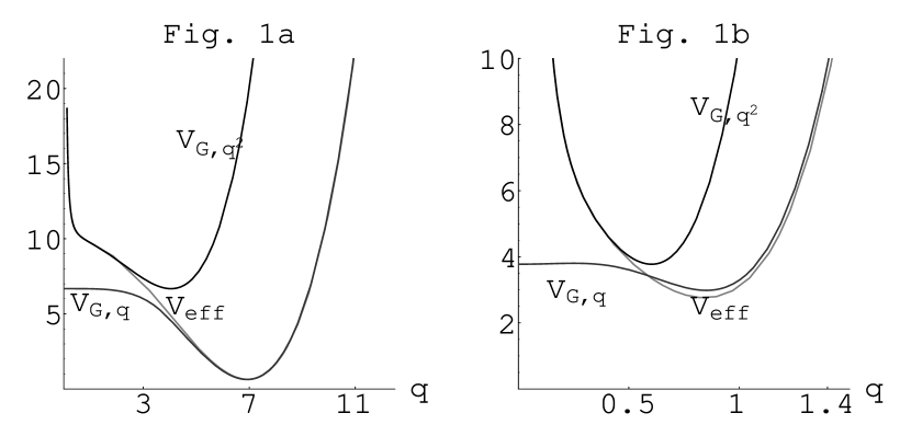
Figure 1: The effective potential as a function of $q$ for the parameters $\lambda=0.1,~{}k=7,~{}m=1$ (a), and $\lambda=123,~{}k=1,~{}m=1$ (b).

In these figures, $V_{eff}=U$, $V_{G,q}$, and $V_{G,q^{2}}$ represent the effective potential  (22), the Gaussian approximated effective potential for $\langle\hat{q}\rangle$, and the Gaussian approximated effective potential for $\langle\hat{q}^{2}\rangle$, respectively. Here, $V_{G,q}$ can be calculated from Eqs. (2.9) and (4.6) of Ref. [3] with slight notational change ($q=\langle\hat{Q}\rangle$) and $V_{G,q^{2}}$ from Eq. (2.9) of Ref. [3] with $\langle\hat{Q}\rangle=0$ and $G\rightarrow q^{2}$. The effective potential, $V_{eff}$, is very close to $V_{G,q^{2}}$ for $q<k/3$, and it becomes close to $V_{G,q}$ for $q>2k/3$. This clearly shows that the initial GP is divided into a DGP, with each packet of the DGP moving as if it is a free GP for large $k$. The value of $y_{v}[\sim 1+\left(\frac{3}{\lambda mq^{6}}\right)^{2/5},$ for $y_{v}\sim 1.]$ is effectively 1 for the most range of $q$ if $k$ is sufficiently large [$\gg(\lambda m)^{-1/6}$], since the characteristic size of $q$ is $O(k)$.

Let us explicitly describe the dynamics of an initial GP with $q=q_{0}~{}(\ll\kappa)$ for the time-dependent potential (1). Because of the transition (as $k(t)$ increase) $y$ eventually goes to 1 for most part of the dynamics. The potential energy difference $\triangle V=V_{eff}(q_{0},y=1)-V_{eff}(q_{0},y=3)>0$ and the presence of kinetic energy in $y$ prevent $q$ from reaching $q_{0}$. The time-dependence of $k(t)$ decreases the total energy so that $q$ oscillates near the true vacuum. We present, in Fig. 2, a solution of the differential equation (14) and its exact numerical solution for the case of $k(t)$ linearly increasing to a finite value for about a half period of $q$.

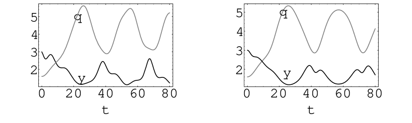
Figure 2: Solution (Left) of Eq. (14) and exact numerical time evolution by wave-function simulation (Right) of $q(t)$ and $y(t)$. In this figure, we set $\lambda=0.0123$, $m=1$, $q_{0}=1.6$, and $y(0)=3$. $k(t)=t/3$ during $0\leq t\leq 15$ and remains constant afterward.

In this example, we do not need the patching process by the wavefunction (15) since states with $y>3$ do not appear. To see the long time behavior of the system, we present one more figure(Fig. 3).

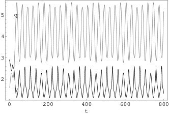
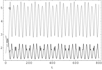
Figure 3: Solution (Left) of Eq. (14) and exact numerical time evolution by wave-function simulation (Right) of $q(t)$ and $y(t)$. In this figure, we set $\lambda=0.0123$, $m=1$, $q_{0}=1.6$, and $y(0)=2.906$. $k(t)=t/3$ during $0\leq t\leq 30$ and remains constant afterward.

The main characteristic feature of the long time behavior is the oscillation of the amplitude of short time oscillation. The error of the oscillation period in Fig. 3 is about 25%. This error comes from the non-exactness of the variational wave-function to the exact time-evolution of the wave-function.

As another example, let us consider the quenched transition potential with $k(t>0)=\kappa$ and $k(t<0)=0$. The discussions above for the time-dependent $k(t)$ transition also applies to the present example. We present a numerical solution of the differential equation (14) and its exact time evolution in Fig. 4.

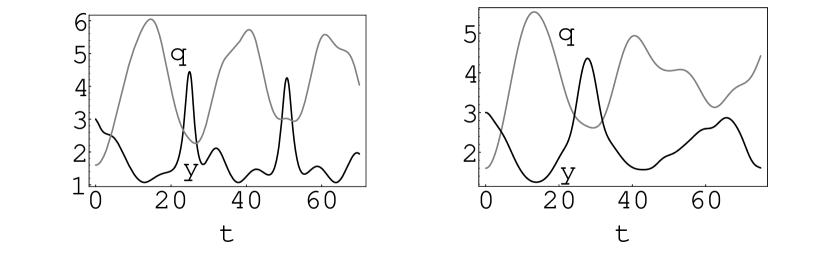
Figure 4: Solution (Left) of Eq. (14) and exact numerical time evolution (Right) of $q(t)$ and $y(t)$ by wave-function simulation. In this figure, we set $\lambda=0.0123$, $\kappa=5$, $m=1$, $q_{0}=1.6$, and $y(0)=3$.

The state with large $y(>3)$ periodically appears. This means that we need the patching process (15) for the time evolution of this system. Comparing the two results in Fig. 4, one may notice the merits and the weakness of the present approach for the quenched transition. The present approach explains the periodic appearance of the large “shape factor” and well presents the period of its occurrence, but the details of the evolution is not exact. This discrepancy is related to the “patched” trial wavefunction (4) and (15) at $y=3$. We have chosen this artificial patching method because of its simplicity. A better approach may be to include the excited states of (4) without introducing the patching, (15). One of the excited states, $\langle Q|\psi_{2},t\rangle=(y-1)^{-1/2}\left(\frac{Q^{2}}{q^{2}(t)}-1\right)\langle Q|\psi,t\rangle$, is an orthonormal wavefunction to $\langle Q|\psi,t\rangle$. Because of the symmetry of the potential (1), the odd function of $q$ cannot contributes to the evolution. One may try the variational method by using the following trial wavefunction:

$$\langle Q|\bar{\psi},t\rangle=\bar{N}^{-1}\left[\langle Q|\psi,t\rangle+z\langle Q|\psi_{2},t\rangle\right],$$ (23)

where $z$ is a complex valued function of time and the normalization factor is $\bar{N}^{2}=1+|z|^{2}$. This wavefunction naturally includes the regions with $y>3$ due to the contribution of the excited state. In this sense, the appearance of large “shape factor” ($>3$) is the signal for the contribution of excited states in the time evolution of the systems. Generally, the accuracy of the approximation (4) increases as the potential varies slowly. We applied the present method to the case of scalar $\phi^{4}$ field theory in Ref. [9], and it would be interesting to apply more realistic quantum mechanical systems in second order phase transition.

Another point we need to speculate is the large $N$ limit. It was shown that the large $N$ wave-function satisfies [10]

$$i\frac{\partial\Phi(z,\tau)}{\partial\tau}=\left[-\frac{1}{2N^{2}}\frac{\partial^{2}}{\partial z^{2}}+u(z,N)\right]\Phi(z,\tau),$$ (24)

where $\tau=Nt$, $\displaystyle r^{2}\equiv\sum_{k=1}^{N}x_{k}^{2}=Nz^{2}$, and $u(z,N)=\frac{(N-1)(N-3)}{8N^{2}z^{2}}+\frac{g}{8}(z^{2}-z_{0}^{2})^{2}$. The present approximation for symmetric state is given by

$$\Gamma=\int d\tau\langle\psi,\tau|i\partial_{\tau}-\frac{1}{2N^{2}}\Pi^{2}-u(z,N)|\psi,\tau\rangle.$$ (25)

This is the same as Eq. (3) with the change of parameters $t,Q,m,V(Q,t)\rightarrow\tau,z,N^{2},u(z,N)$. With the use of the trial wave-function (4) in (25) the expectation value of $\frac{1}{2N^{2}}\Pi^{2}$ is given by

$$2y\left[y-\frac{y-3}{Y+1}\right]\frac{q^{6}\Pi^{2}}{N^{2}}+\frac{2q^{2}p^{2}}{N^{2}}-\frac{4yq^{4}\Pi p}{N^{2}}+\frac{V_{F}(y)}{8N^{2}},$$ (26)

where the first three terms in Eq. (26) are $O(1)$, and in the large $N$ limit the quantum mechanical effects on the potential $\frac{V_{F}(y)}{8N^{2}}$ effectively vanishes as $O(1/N^{2})$. In the absence of this quantum mechanical term, the equations of motion in the large $N$ limits for the present quartic exponential approximation with $y=1$ is the same as that of the Gaussian approximation centered at $z\neq 0$. Since the Gaussian approximation was proven to be the same as large $N$ approximation [11], the present approximation is equivalent to the large $N$ approximation for $N\rightarrow\infty$.

Acknowledgments
 
This work was supported in part by Korea Research Foundation under Project number KRF-2001-005-D2003 (H.-C.K. and J.H.Y.).

References

[1]
R. Jackiw and A. K. Kerman, Phys. Lett. A 71, 158 (1979).
[2]
L. Polley and U. Ritschel, ”A step beyond the Gaussian
Approximation in Yang-Mills Theory”, Proceedings of the
International Workshop on Variational Calculations in Quantum
Field Theory, World Scientific, Wangerooge, West Germany, 1-4
Sep. (1987).
[3]
F. Cooper, S.-Y. Pi, and P. N. Stancioff, Phys. Rev. D 34,
3831 (1986).
[4]
G. J. Cheetham and E. J. Copeland, Phys. Rev. D 53, 4125
(1996).
[5]
S. W. Hawking and I. G. Moss, Nucl. Phys. B 224 180 (1983).
[6]
has no upper limit. As an example, we consider .
The shape factor for this packet is , where
, and .
[7]
F. J. Alexander, S. Habib, and A. Kovner, Phys. Rev.
E 48, 4284 (1993).
[8]
Part of this formula for can be found in the literature
Gradshteyn and Ryzhik, Table of integrals, Series, and
Products, 5th eds. Academic Press. To give another half of the
proof for , we use differential equation, , coming from . This differential equation and the boundary conditions at
uniquely determine .
[9]
Hyeong-Chan Kim and Jae Hyung Yee, “Zero mode in the time-dependent
symmetry breaking of theory”, hep-th/0306081, submitted
to Phys. Rev. D.
[10]
B. Mihaila, T. Athan, F. Cooper, J. Dawson, and S. Habib, Phys. Rev. D 62, 125015 (2000).
[11]
F. Cooper and E. Mottola, Phys. Rev. D 36, 3114 (1987); P. M.
Stevenson, B. Allès, and R. Tarrach, Phys. Rev. D 35, 2407
(1987).