Neil R. Constable$\,{}^{a}$, Johanna Erdmenger$\,{}^{b}$, Zachary Guralnik$\,{}^{b}$ and Ingo Kirsch$\,{}^{b}$

^a Center for Theoretical Physics and Laboratory for Nuclear Science

Massachusetts Institute of Technology

77 Massachusetts Avenue

Cambridge, MA 02139, USA

^b Institut für Physik

Humboldt-Universität zu Berlin

Invalidenstraße 110

D-10115 Berlin, Germany

Abstract

We describe intersecting M5-branes, as well as M5-branes wrapping the holomorphic curve $xy=c$, in terms of a limit of a defect conformal field theory with two-dimensional $(4,0)$ supersymmetry. This defect CFT describes the low-energy theory of intersecting D3-branes at a $\mathbb{C}^{2}/\mathbb{Z}_{k}$ orbifold. In an appropriate $k\rightarrow\infty$ limit, two compact spatial directions are generated. By identifying moduli of the M5-M5 intersection in terms of those of the defect CFT, we argue that the $SU(2)_{L}$ R-symmetry of the $(4,0)$ defect CFT matches the $SU(2)$ R-symmetry of the ${\cal N}=2,d=4$ theory of the M5-M5 intersection. We find a ’t Hooft anomaly in the $SU(2)_{L}$ R-symmetry, suggesting that tensionless strings give rise to an anomaly in the $SU(2)$ R-symmetry of intersecting M5-branes.

1 Introduction

In recent years string theory has suggested the existence of novel interacting conformal theories in diverse dimensions. In many cases, a Lagrangian description of these theories is lacking. A particularily interesting example is the six-dimensional theory with $(2,0)$ supersymmetry describing the low energy limit of IIB string theory on an $A_{n}$ singularity [1], as well as the decoupling limit of multiple parallel M5-branes [2]. Although this theory is believed to be a local quantum field theory, obstructions to finding a Lagrangian description arise because of difficulties in constructing a non-abelian generalization of a chiral two-form (see for example [3]). The spectrum includes tensionless BPS strings, which are in some sense the “off-diagonal” excitations of the non-abelian chiral two-form. Until recently, the only known formulation of theory was in terms of a M(atrix) model describing its discrete light cone quantization [4]. More recently, an alternative formulation was found [5, 6] using a procedure known as (de)construction [7, 8]. In this approach, the $(2,0)$ theory is obtained as a limit of ${\cal N}=2,d=4$ superconformal Yang-Mills theories described by a circular quiver diagram. This limit entails taking the number $k$ of nodes in the diagram to infinity, while scaling the gauge coupling as $\sqrt{k}$. At the same time one goes increasingly far out onto the Higgs branch, on which the gauge group is broken from $SU(N)^{k}$ to the diagonal $SU(N)$. The quiver diagram can then be viewed a discretization of an extra spatial circle, which is believed to become continuous as $k\rightarrow\infty$. The S-duality of the theory implies the generation of yet another discretized circular dimension which also becomes continuous as $k\rightarrow\infty$.

Even more poorly understood than the $(2,0)$ theory is the one which describes the low energy dynamics of intersecting M5-branes. In addition to a non-abelian chiral two-form, this theory has tensionless strings localized at the intersection corresponding to M2-branes stretched between the M5-branes [9]. These tensionless strings are in some sense fundamental, as they are not excitations of a chiral two-form. The only known formulation of the M5-M5 intersection is the DLCQ M(atrix) description proposed in [10].

Here we shall present the (de)construction of the M5-M5 intersection, which is a natural extension of the (de)construction of parallel M5-branes discussed in [5, 6]. This will be accomplished by taking a $k\rightarrow\infty$ limit of the theory describing intersecting D3-branes at a $\mathbb{C}^{2}/\mathbb{Z}_{k}$ orbifold. At a certain point in the moduli space, two compact latticized extra dimensions are generated. In an appropriate $k\rightarrow\infty$ limit, we expect that the extra directions become continuous, such that the intersection of four-dimensional world volumes over $1+1$ dimensions becomes an intersection of six-dimensional world volumes over $1+3$ dimensions.

The infrared dynamics of the D3-D3 intersection at a $\mathbb{C}^{2}/\mathbb{Z}_{k}$ orbifold is described by a defect conformal field theory with two-dimensional $(4,0)$ supersymmetry. This theory belongs to an interesting class of conformal field theories with defects which have recently been studied in a variety of contexts [11, 12, 13, 14, 15, 16, 17, 18, 19, 20, 21, 22, 23, 24]. The action of this $(4,0)$ theory is readily constructed in $(2,0)$ superspace, starting from the action for the D3-D3 intersection in flat space which was constructed in [24]. The field content of the $(4,0)$ theory is summarized by a quiver (or “moose”) diagram consisting of two concentric rings, and spokes stretching between the inner and outer rings. For large $k$ this gives rise to a discretized version of the field theory corresponding to the low-energy limit of the M5-M5 intersection. The spokes in the quiver diagram will be seen to correspond to strings localized at the M5-brane intersection.

Moreover, we examine the relation between the moduli space of vacua of the $(4,0)$ defect conformal field theory and that of the M5-M5 intersection. On a particular part of the Higgs branch of the defect CFT, the resolution of the intersection to a holomorphic curve $xy=c$ can be seen very explicitly from F-flatness conditions. This point in the Higgs branch corresponds to a vacuum of the M5-M5 theory in which tensionless strings have condensed. By going to another point on the Higgs branch of the defect CFT for which the string tension in the M5-M5 theory is non-zero, we will be able to match the $SU(2)_{L}$ R-symmetry of the $(4,0)$ theory with the $SU(2)$ R-symmetry of the M5-M5 intersection, which has ${\cal N}=2,d=4$ supersymmetry.

The chiral nature of the theory which deconstructs the M5-M5 intersection is a bit surprising, and should have physical consequences. Using the $(4,0)$ dCFT, we will search for ’t Hooft anomalies in the R-symmetry of the M5-M5 intersection. One reason to be interested in R-symmetry anomalies is that they are related by supersymmetry to the Weyl anomaly and to black hole entropy [25, 26]. Their existence also influences the low energy effective theory at certain points in the moduli space through Wess-Zumino terms which appear upon integrating out degrees of freedom responsible for the anomaly [27]. It turns out there is a ’t Hooft anomaly in the $SU(2)_{L}$ R-symmetry of the $(4,0)$ dCFT, under which only left handed two-dimensional fermions are charged. Assuming a finite continuum limit, this anomaly should be interpreted as an $SU(2)$ R-symmetry anomaly due to tensionless strings in four dimensions. Although there are no $SU(2)$ anomalies in local quantum field theories in four dimensions, the possibility is not excluded for a four-dimensional theory of tensionless strings. Unfortunately we can not yet conclusively state that this occurs, since we have not obtained the continuum limit of the anomaly.

Upon coupling to eleven-dimensional supergravity, a ’t Hooft anomaly in the $SU(2)$ R-symmetry would become an anomaly in diffeomorphisms of the normal bundle. This should presumably be cancelled by a diffeomorphism anomaly due to Chern-Simons terms in the supergravity action in the presence of magnetic (M5-brane) sources. We will briefly comment on the contribution of Chern-Simons terms.

A similar anomaly is known to exist for the $Spin(5)$ R-symmetry of the six-dimensional $(2,0)$ theory describing parallel M5-branes [25, 26, 28, 29, 30, 31]. The anomaly can be directly calculated in the abelian $(2,0)$ theory, which was first done in [28]. However, for multiple M5-branes the anomaly has only been indirectly calculated from the assumption of anomaly cancellation in M-theory [25, 26]. For $N$ M5-branes, the anomaly coefficient is proportional to $N^{3}$ at large $N$, which is consistent with the Weyl anomaly [32] and black hole entropy [26, 33, 34] calculations. A direct calculation of the anomaly based on (de)construction should in principle be possible, but seems to be difficult because the $SO(5)$ R-symmetry is realized only in the $k\rightarrow\infty$ limit. In the case of intersecting five-branes, the R-symmetry is realized even for finite $k$, making the anomaly calculation more tractable.

The organization of this paper is as follows. In section 2 we review the theory of the D3-D3 intersection in flat space, which was discussed in [24]. This action is presented in $(2,2)$ superspace. In section 3 we find the quiver diagram for the D3-D3 intersection at a $\mathbb{C}^{2}/\mathbb{Z}_{k}$ orbifold, and present the action in $(2,0)$ superspace. In section 4 we show how the theory corresponding to the M5-M5 intersection arises in an appropriate $k\rightarrow\infty$ limit. We identify the strings localized at the M5-M5 intersection. Moreover, we identify the moduli and R-symmetries of the M5-M5 intersection in the quiver theory, and discuss the ’t Hooft anomaly in the $SU(2)$ R-symmetry. In section 5 we suggest some open problems.

2 D3-branes intersecting in flat space

Before writing the action of intersecting D3-branes at a $\mathbb{C}^{2}/\mathbb{Z}_{k}$ orbifold, it is useful to first write the action of intersecting D3-branes in flat space. We shall consider a stack of $N$ parallel D3-branes in the directions $0123$ intersecting an orthogonal stack of $N^{\prime}$ D3^′-branes in the directions $0145$. The action has the form

$$S=S_{\rm D3}+S_{\rm D3^{\prime}}+S_{\rm D3-D3^{\prime}}\,.$$ (2.1)

The components $S_{\rm D3}$ and $S_{\rm D3}$ each correspond to a four dimensional ${\cal N}=4$ theory. The term $S_{\rm D3-D3^{\prime}}$ contains couplings to a two-dimensional $(4,4)$ hypermultiplet, leaving only $(4,4)$ supersymmetry unbroken. The action was explicitly constructed in $(2,2)$ superspace in [24], to which we refer the reader for a more detailed discussion.

It is convenient to define the coordinates

$$z^{\pm}=X^{0}\pm X^{1}\,,\qquad x=X^{2}+iX^{3}\,,\qquad y=X^{4}+iX^{5}\,.$$ (2.2)

The two-dimensional $(2,2)$ superspace is spanned by $(z,\bar{z},\theta^{+},\theta^{-},\bar{\theta}^{+},\bar{\theta}^{-})$. The four-dimensional fields corresponding to D3-D3 strings are described by $(2,2)$ superfields with extra continuous labels $x,\bar{x}$, while fields associated to the D$3^{\prime}$-D$3^{\prime}$ strings have the extra labels $y,\bar{y}$. Although the four-dimensional parts of the action will look strange in $(2,2)$ superspace, this notation makes sense since only a two-dimensional supersymmetry is preserved. The fields associated with D3-D$3^{\prime}$ strings are trapped at the intersection and have no extra continuous label.

Let us first consider $S_{\rm D3}$, which involves $(2,2)$ superfields of the form $F(z^{+},z^{-},\theta,\bar{\theta}|x,\bar{x})$. The required superfields are a vector superfield $V$, together with three adjoint chiral superfields $Q_{1},Q_{2}$ and $\Phi$. The gauge connections $A_{0,1}$ of the $(2,2)$ vector multiplet and the complex scalar $\phi$ of the $(2,2)$ chiral field $\Phi$ combine to give the four gauge connections of the four-dimensional ${\cal N}=4$ theory. From $V$ one can build a twisted chiral (field strength) multiplet,

$$\Sigma\equiv\left\{\bar{\cal D}_{+},{\cal D}_{-}\right\}\,,\quad\bar{\cal D}_{+}=e^{-V}\bar{D}_{+}e^{V}\,,\quad{\cal D}_{-}=e^{V}D_{-}e^{-V}\,,$$ (2.3)

satisfying $\bar{\cal D}_{+}\Sigma={\cal D}_{-}\Sigma=0$. The scalar components of $\Sigma,Q_{1}$ and $Q_{2}$ combine to give the six adjoint scalars of the four-dimensional ${\cal N}=4$ theory. The field content of the second D3-brane (D$3^{\prime})$ is identical to that of the first D3-brane with the replacements

$$x\rightarrow y\,,\quad V\rightarrow{\cal V}\,,\quad\Sigma\rightarrow\Omega\,,\quad Q_{i}\rightarrow S_{i}\,,\quad\Phi\rightarrow\Upsilon\,.$$ (2.4)

The fields corresponding to D3-D$3^{\prime}$ strings are the chiral multiplets $B$ and $\tilde{B}$ in the $(N,\bar{N}^{\prime})$ and $(\bar{N},N^{\prime})$ representations of the $SU(N)\times SU(N^{\prime})$ gauge group. Together they form a $(4,4)$ hypermultiplet.

The components of the action are as follows:

$$\ S_{\rm D3}=\, \frac{1}{g^{2}}\int d^{2}zd^{2}xd^{4}\theta{\rm\,tr}\left(\Sigma^{\dagger}\Sigma+(\partial_{x}+g\bar{\Phi})e^{gV}(\partial_{\bar{x}}+g\Phi)e^{-gV}+\sum_{i=1,2}e^{-gV}\bar{Q}_{i}e^{gV}Q_{i}\right)$$

$$+ \int d^{2}zd^{2}xd^{2}\theta\epsilon_{ij}{\rm\,tr\,}Q_{i}[\partial_{\bar{x}}+g\Phi,Q_{j}]+c.c\quad,$$ (2.5)

$$S_{\rm D3^{\prime}}=\, \frac{1}{g^{2}}\int d^{2}zd^{2}yd^{4}\theta{\rm\,tr}\left(\Omega^{\dagger}\Omega+(\partial_{y}+g\bar{\Upsilon})e^{g{\cal V}}(\partial_{\bar{y}}+g\Upsilon)e^{-g{\cal V}}+\sum_{i=1,2}e^{-g{\cal V}}\bar{S}_{i}e^{g{\cal V}}S_{i}\right)$$

$$+ \int d^{2}zd^{2}yd^{2}\theta\epsilon_{ij}{\rm\,tr\,}S_{i}[\partial_{\bar{y}}+g\Upsilon,S_{j}]+c.c\quad,$$ (2.6)

$$S_{\rm D3-D3^{\prime}}= \int d^{2}zd^{4}\theta{\rm\,tr}\left(e^{-g\cal V}\bar{B}e^{gV}B+e^{-gV}\bar{\tilde{B}}e^{g\cal V}\tilde{B}\right)$$

$$+ \frac{ig}{{2}}\int d^{2}zd^{2}\theta{\,\rm tr}\left(B\tilde{B}Q_{1}-\tilde{B}BS_{1}\right)+c.c.\quad,$$ (2.7)

with $d^{4}\theta=\frac{1}{4}d\theta^{+}d\theta^{-}d\bar{\theta}^{+}d\bar{\theta}^{-}$ and $d^{2}\theta=\frac{1}{2}d\theta^{+}d\theta^{-}$.

The fact that $S_{\rm D3}$ (or $S_{\rm D3^{\prime}}$) describe theories with four-dimensional Lorentz invariance, namely ${\cal N}=4$ super Yang-Mills, can be seen in component notation after integrating out auxiliary fields. For instance the kinetic term ${\rm tr}\,\partial_{\mu}\bar{q}_{1}\partial^{\mu}q_{1}$ with $\mu=0,1,2,3$, arises from a combination of the $(2,2)$ K$\ddot{{\rm a}}$hler term ${\rm tr}\,\bar{Q}_{1}Q_{1}$ and the superpotential term ${\rm tr}\,Q^{1}\partial_{z}Q^{2}$.

The fields $B$ and $\tilde{B}$ acquire masses from expectation values for $s_{1}-q_{1}$, the lowest component of the superfield $S_{1}-Q_{1}$, as well as from expectation values for $\sigma-\sigma^{\prime}$, where $\sigma$ and $\sigma^{\prime}$ are the complex scalars in $V$ (or $\Sigma$) and $\cal V$ (or $\Omega$). The scalar $s_{1}-q_{1}$ describes fluctuations in the $u=X_{6}+iX_{7}$ direction, and $\sigma-\sigma^{\prime}$ describes fluctuations in the $w=X_{8}+iX_{9}$ direction. Both $u$ and $w$ are transverse to both stacks of D3-branes. On the Higgs branch the orthogonal D3-branes intersect and the scalars $s_{1}-q_{1}$ and $\sigma-\sigma^{\prime}$ vanish. The scalar components $b$ and $\tilde{b}$ of $B$ and $\tilde{B}$ have (classical) expectation values on the Higgs branch. The scalar components $s_{2}$ and $q_{2}$ of $S_{2}$ and $Q_{2}$ also have expectation values given by the vanishing of the F-terms for $S^{1}$ and $Q^{1}$:

$$\frac{\partial W}{\partial q_{1}}=\partial_{\bar{x}}q_{2}-g\delta^{2}(x)b\tilde{b} =0\,,\qquad\frac{\partial W}{\partial s_{1}}=\partial_{\bar{y}}s_{2}-g\delta^{2}(y)\tilde{b}b=0\,.$$ (2.8)

With the geometric identifications $q_{2}\sim y/\alpha^{\prime}$ and $s_{2}\sim x/\alpha^{\prime}$, the solutions of these equations give rise to holomorphic curves of the form $xy=c\alpha^{\prime}$, when $2\pi ic=gb\tilde{b}=g\tilde{b}b$.

The geometric symmetries of the D3-D3 intersection are as follows. There is an $SU(2)_{L}\times SU(2)_{R}$ R-symmetry corresponding to rotations in the $6789$ directions transverse to all D3-branes. Additionally there are $U(1)$ symmetries corresponding to rotations in the $23$ and $45$ (or $x$ and $y$) planes. The charges of the various fields under these symmetries are summarized in table 1.

$(4,4)$	$(2,2)$	$(2,0)$	components	$(j_{L},j_{R})$	$J_{23}$	$J_{45}$
			$\sigma,q_{1}$	$(\frac{1}{2},\frac{1}{2})$	$0$	$0$
Vector	$Q_{1},\Sigma$	$Q_{1},\Lambda^{Q_{1}}_{-}$	$\psi_{q_{1}}^{+},\bar{\lambda}_{\sigma}^{+}$	$(0,\frac{1}{2})$	$\frac{1}{2}$	$-\frac{1}{2}$
		$\Theta_{V},V$	$\psi_{q_{1}}^{-},\bar{\lambda}_{\sigma}^{-}$	$(\frac{1}{2},0)$	$\frac{1}{2}$	$-\frac{1}{2}$
			$v_{0},v_{1}$	$(0,0)$	$0$	$0$
			$\phi$	$(0,0)$	$-1$	$0$
Hyper	$Q_{2},\Phi$	$Q_{2},\Lambda_{-}^{Q_{2}}$	$q_{2}$	$(0,0)$	$0$	$1$
		$\Phi,\Lambda_{-}^{\Phi}$	$\psi_{\phi}^{+},\bar{\psi}_{q_{2}}^{+}$	$(\frac{1}{2},0)$	$-\frac{1}{2}$	$-\frac{1}{2}$
			$\psi_{\phi}^{-},\bar{\psi}_{q_{2}}^{-}$	$(0,\frac{1}{2})$	$-\frac{1}{2}$	$-\frac{1}{2}$
			$b$	$(0,0)$	$-\frac{1}{2}$	$\frac{1}{2}$
Hyper	$B,\tilde{B}$	$B,\Lambda^{B}_{-}$	$\tilde{b}$	$(0,0)$	$-\frac{1}{2}$	$\frac{1}{2}$
		$\tilde{B},\tilde{\Lambda}^{\tilde{B}}_{-}$	$\psi_{b}^{+},\bar{\psi}_{\tilde{b}}^{+}$	$(\frac{1}{2},0)$	$0$	$0$
			$\psi_{b}^{-},\bar{\psi}_{\tilde{b}}^{-}$	$(0,\frac{1}{2})$	$0$	$0$
			$\omega,s_{1}$	$(\frac{1}{2},\frac{1}{2})$	$0$	$0$
Vector	$S_{1},\Omega$	$S_{1},\Lambda^{S_{1}}_{-}$	$\psi_{s_{1}}^{+},\bar{\psi}_{\omega}^{+}$	$(0,\frac{1}{2})$	$\frac{1}{2}$	$-\frac{1}{2}$
		$\Theta_{\cal V},{\cal V}$	$\psi_{s_{1}}^{-},\bar{\psi}_{\omega}^{-}$	$(\frac{1}{2},0)$	$\frac{1}{2}$	$-\frac{1}{2}$
			$a_{0},a_{1}$	$(0,0)$	$0$	$0$
			$\upsilon$	$(0,0)$	$0$	$1$
Hyper	$S_{2},\Upsilon$	$S_{2},\Lambda_{-}^{S_{2}}$	$s_{2}$	$(0,0)$	$-1$	$0$
		$\Upsilon,\Lambda_{-}^{\Upsilon}$	$\lambda_{\upsilon}^{+},\bar{\psi}_{s_{2}}^{+}$	$(\frac{1}{2},0)$	$\frac{1}{2}$	$\frac{1}{2}$
			$\lambda_{\upsilon}^{-},\bar{\psi}_{s_{2}}^{-}$	$(0,\frac{1}{2})$	$\frac{1}{2}$	$\frac{1}{2}$

Table 1: Field content of the D3-D3 intersection.

The $U(1)$ symmetries generated by $J_{45}$ and $J_{23}$ are manifest in $(2,2)$ superspace. The $U(1)$ generated by $J_{45}$ has the following action:

$$\theta^{+}\rightarrow e^{i\alpha/2}\theta^{+}\,, B\rightarrow e^{i\alpha/2}B\,, Q_{2}\rightarrow e^{i\alpha}Q_{2}\,,$$

$$\theta^{-}\rightarrow e^{i\alpha/2}\theta^{-}\,, \tilde{B}\rightarrow e^{i\alpha/2}\tilde{B}\,, \Upsilon\rightarrow e^{+i\alpha}\Upsilon\,,$$

$$y\rightarrow e^{i\alpha}y\,,$$ (2.9)

with all remaining fields being singlets. The $U(1)$ generated by $J_{23}$ acts as

$$\theta^{+}\rightarrow e^{-i\alpha/2}\theta^{+}\,, B\rightarrow e^{-i\alpha/2}B\,, S_{2}\rightarrow e^{-i\alpha}S_{2}\,,$$

$$\theta^{-}\rightarrow e^{-i\alpha/2}\theta^{-}\,, \tilde{B}\rightarrow e^{-i\alpha/2}\tilde{B}\,, \Phi\rightarrow e^{-i\alpha}\Phi\,,$$

$$x\rightarrow e^{-i\alpha}x\,.$$ (2.10)

3 D3-D3 intersection at a $\mathbb{C}^{2}/\mathbb{Z}_{k}$ orbifold

To (de)construct the theory of the M5-M5 intersection, we shall consider a pair of intersecting stacks of D3-branes at an $\mathbb{C}^{2}/\mathbb{Z}_{k}$ orbifold point. One set of D3-branes is located at $X^{4,5,6,7,8,9}=0$ while the other set of ${\rm D3}^{\prime}$ branes is located at $X^{2,3,6,7,8,9}=0$. The $\mathbb{C}^{2}/\mathbb{Z}_{k}$ is spanned by the coordinates $u=X^{6}+iX^{7}$ and $w=X^{8}+iX^{9}$ subject to the orbifold condition $u\sim\xi u,w\sim\xi^{-1}w$ where $\xi=\exp(2\pi i/k)$. Before orbifolding, the theory of intersecting D3-branes has $(4,4)$ supersymmetry with an $SU(2)_{L}\times SU(2)_{R}$ R-symmetry. The $SU(2)_{L}\times SU(2)_{R}$ component of the R-symmetry acts as an $SO(4)$ transformation on the real components of $u$ and $w$, which are the coordinates $X^{6,7,8,9}$. The orbifold breaks $SU(2)_{L}\times SU(2)_{R}$ to $SU(2)_{L}$, under which the pair $u,w^{*}$ transform as a doublet. Moreover, the supersymmetry is broken from $(4,4)$ to $(4,0)$. The chiral nature of this theory will prove important later when we find evidence that tensionless strings give rise to a ’t Hooft anomaly in an R-symmetry of the M5-M5 intersection.

3.1 Orbifold projection

The Lagrangian describing the D3-D3 intersection in the $\mathbb{C}^{2}/\mathbb{Z}_{k}$ orbifold can be obtained from the action of the D3-D3 intersection in flat space given in (2) - (2). Following refs. [37, 38] we start with $Nk$ D3-branes intersecting $N^{\prime}k$ D3-branes in a flat background and project out the degrees of freedom which are not invariant under the $\mathbb{Z}_{k}$ orbifold group, which is generated by a combination of a gauge symmetry and an R-symmetry. An important constraint on the orbifold action is that the theory on each stack of D3 branes (ignoring strings connected to the other stack) should be the ${\cal N}=2,d=4$ super Yang-Mills theory described by the quiver in figure 1, with gauge group $SU(N)^{k}$ or $SU(N^{\prime})^{k}$.

Figure 1: Quiver diagram for parallel D3-branes at a $\mathbb{C}^{2}/\mathbb{Z}_{k}$ orbifold (here $k=8$). Each node corresponds to an ${\cal N}=2$ vector multiplet, while double lines between neighboring nodes correspond to an $\mathcal{N}=2$ hypermultiplet.

The orbifold action which gives the quiver of figure 1 for both the D3 and the D3^′ degrees of freedom separately, and breaks the $SU(2)_{L}\times SU(2)_{R}$ R-symmetry to $SU(2)_{L}$ is as follows. The embedding of the $\mathbb{Z}_{k}$ orbifold group in the $U(Nk)$ and $U(N^{\prime}k)$ gauge groups is given by

$$g(\xi) =\begin{pmatrix}I_{N\times N}&&&\\ &\xi I_{N\times N}&&\\ &&\xi^{2}I_{N\times N}&\\ &&&\ddots\end{pmatrix}\,,$$ (3.1)

$$g^{\prime}(\xi) =\begin{pmatrix}I_{N^{\prime}\times N^{\prime}}&&&\\ &\xi I_{N^{\prime}\times N^{\prime}}&&\\ &&\xi^{2}I_{N^{\prime}\times N^{\prime}}&\\ &&&\ddots\end{pmatrix}\,,$$ (3.2)

where $\xi$ is the generator $\exp(2\pi i/k)$ of $\mathbb{Z}_{k}$. The embedding of the $\mathbb{Z}_{k}$ orbifold group in the R-symmetry is given by

$$h(\xi)=e^{i\pi\sigma^{3}/k}\,,$$ (3.3)

where $h$ belongs to $SU(2)_{R}$. The field theory describing the D3-D$3^{\prime}$ intersection at the orbifold is then obtained from that of the D3-D$3^{\prime}$ intersection in flat space by projecting out fields which are not invariant under the orbifold action. The result is an $SU(N)^{k}\times SU(N^{\prime})^{k}$ gauge theory with $(4,0)$ supersymmetry and $SU(2)_{L}\times U(1)$ R-symmetry.

In $(2,2)$ superspace, the orbifold acts on superspace coordinates as

$$\theta^{-}\rightarrow\xi\theta^{-}\,,$$ (3.4)

but trivially on $\theta^{+}$. On the $(2,2)$ superfields the orbifold acts as

$${\rm D3}: V\rightarrow g(\xi)Vg^{\dagger}(\xi)\,, \Sigma\rightarrow\xi^{-1}g(\xi)\Sigma g^{\dagger}(\xi)\,,$$

$$Q_{1}\rightarrow\xi g(\xi)Q_{1}g^{\dagger}(\xi)\,, Q_{2}\rightarrow g(\xi)Q_{2}g^{\dagger}(\xi)\,,$$

$$\Phi\rightarrow g(\xi)\Phi g^{\dagger}(\xi)\,,$$

$${\rm D3}^{\prime}: {\cal V}\rightarrow g^{\prime}(\xi){\cal V}g^{\prime\dagger}(\xi)\,, \Omega\rightarrow\xi^{-1}g^{\prime}(\xi)\Omega g^{\prime\dagger}(\xi)\,,$$

$$S_{1}\rightarrow\xi g^{\prime}(\xi)S_{1}g^{\prime\dagger}(\xi)\,, S_{2}\rightarrow g^{\prime}(\xi)S_{2}g^{\prime\dagger}(\xi)\,,$$

$$\Upsilon\rightarrow g^{\prime}(\xi)\Upsilon g^{\prime\dagger}(\xi)\,,$$

$${\rm D3-D3^{\prime}}: B\rightarrow g(\xi)Bg^{\prime\dagger}(\xi)\,, \tilde{B}\rightarrow g^{\prime}(\xi)\tilde{B}g^{\dagger}(\xi)\,,$$ (3.5)

with $g$, $g^{\prime}$ as in (3.1), (3.2). Starting with the action (2) - (2) and projecting out the degrees of freedom which are not invariant under (3.5) will give a $(4,0)$ supersymmetric action with manifest $(2,0)$ supersymmetry.

To illustrate how the orbifold acts on components, we consider the action (3.5) on the $(2,2)$ twisted superfield $\Sigma$. On the bosonic components, this corresponds to

$$\sigma \sim\xi^{-1}g(\xi)\sigma g^{\dagger}(\xi)\,,\quad F_{01}\sim g(\xi)F_{01}g^{\dagger}(\xi)\,.$$ (3.6)

This is consistent with the fact that the field $\sigma$ characterizes fluctuations transverse to both D3-branes, i.e. fluctuations in the orbifold directions. This field is naturally associated with fluctuations in the $w=X^{8}+iX^{9}$ directions which satisfy the orbifold condition $w\sim\xi^{-1}w$. Upon projecting out the parts which are not invariant under the orbifold, $\sigma$ becomes a set of $k$ bifundamentals in the representations $(\cdots N,\bar{N},\cdots)$ of $SU(N)^{k}$. These bifundamental fields are written as $\sigma_{j,j+1}$, where $j=1\cdots k$ and the first(second) index labels the gauge group with respect to which the field is a fundamental (antifundamental). Fields which are adjoints with respect to one of the factors will be written with a single index.

3.2 Quiver action in two-dimensional $(2,0)$ superspace

Since the $(4,4)$ supersymmetry of the action (2) - (2) is broken down to $(4,0)$ by the orbifold, an adequate formulation of the corresponding quiver gauge theory is best given in $(2,0)$ superspace. In order to project out the degrees of freedom which are not invariant under the orbifold, we rewrite the parent action using manifest $(2,0)$ supersymmetry. To this end, we decompose the $(2,2)$ superfields under $(2,0)$ supersymmetry. The decomposition of the $(2,2)$ superfields is as follows (see for instance [39, 40]):

i) $(2,2)$ vector $\rightarrow$ $(2,0)$ vector $+$ $(2,0)$ chiral,

ii) $(2,2)$ chiral $\rightarrow$ $(2,0)$ chiral $+$ $(2,0)$ Fermi.

These $(2,0)$ superfields have the following component decomposition:

i) $(2,0)$ vector superfield $V$: two gauge connections $A_{0},A_{1}$ and one fermion $\chi_{-}$,

ii) $(2,0)$ chiral superfields $\Phi$: one complex scalar $\phi$ and a fermion $\psi_{+}$,

iii) $(2,0)$ fermi superfields $\Lambda$: one chiral fermion $\lambda_{-}$. The full expansion of this anticommuting superfield contains an auxiliary field and a holomorphic function of $(2,0)$ chiral superfields.

For the theory given by the action (2) - (2), the decomposition of the $(2,2)$ superfields of the D3-D3 intersection in flat space gives the following $(2,0)$ superfields (we shall henceforward write $(2,2)$ superfields in boldface):

$${\rm D3}: {\bf Q}_{1}\rightarrow Q_{1},\Lambda^{Q_{1}}, {\bf Q}_{2}\rightarrow Q_{2},\Lambda^{Q_{2}}, {\bf\Phi}\rightarrow\Phi,\Lambda^{\Phi}, {\bf V}\rightarrow V,\Theta_{V}\,,$$

$${\rm D3}^{\prime}: {\bf S}_{1}\rightarrow S_{1},\Lambda^{S_{1}}, {\bf S}_{2}\rightarrow S_{2},\Lambda^{S_{2}}\,, {\bf\Upsilon}\rightarrow\Upsilon,\Lambda^{\Upsilon}, {\bf{\cal V}}\rightarrow{\cal V},\Theta_{\cal V}\,,$$

$${\rm D3}-{\rm D3}: {\bf B}\rightarrow B,\Lambda^{B}, \tilde{\bf B}\rightarrow\tilde{B},\Lambda^{\tilde{B}}\,.$$ (3.7)

Since we wish to obtain the action for the D3-D3 intersection at the $\mathbb{C}^{2}/\mathbb{Z}_{k}$ singularity in $(2,0)$ superspace, we write the orbifold action (3.4), (3.5) in $(2,0)$ superspace. In terms of the $(2,0)$ decomposition, the orbifold acts as follows:

$${\rm D3}: Q_{1}\rightarrow\xi g(\xi)Q_{1}g^{\dagger}(\xi)\,,\quad \Lambda^{Q_{1}}\rightarrow g(\xi)\Lambda^{Q_{1}}g^{\dagger}(\xi)\,,$$

$$Q_{2}\rightarrow g(\xi)Q_{2}g^{\dagger}(\xi)\,,\quad \Lambda^{Q_{2}}\rightarrow\xi^{-1}g(\xi)\Lambda^{Q_{2}}g^{\dagger}(\xi)\,,$$

$$\Phi\rightarrow g(\xi)\Phi g^{\dagger}(\xi)\,,\quad \Lambda^{\Phi}\rightarrow\xi^{-1}g(\xi)\Lambda^{\Phi}g^{\dagger}(\xi)\,,$$

$$V\rightarrow g(\xi)Vg^{\dagger}(\xi)\,,\quad \Theta_{V}\rightarrow\xi^{-1}g(\xi)\Theta_{V}g^{\dagger}(\xi)\,,$$

$${\rm D3}^{\prime}: S_{1}\rightarrow\xi g^{\prime}(\xi)S_{1}g^{\prime\dagger}(\xi)\,,\quad \Lambda^{S_{1}}\rightarrow g^{\prime}(\xi)\Lambda^{S_{1}}g^{\prime\dagger}(\xi)\,,$$

$$S_{2}\rightarrow g^{\prime}(\xi)S_{2}g^{\prime\dagger}(\xi)\,,\quad \Lambda^{S_{2}}\rightarrow\xi^{-1}g^{\prime}(\xi)\Lambda^{S_{2}}g^{\prime\dagger}(\xi)\,,$$

$$\Upsilon\rightarrow g^{\prime}(\xi)\Upsilon g^{\prime\dagger}(\xi)\,,\quad \Lambda^{\Upsilon}\rightarrow\xi^{-1}g^{\prime}(\xi)\Lambda^{\Upsilon}g^{\prime\dagger}(\xi)\,,$$

$${\cal V}\rightarrow g^{\prime}(\xi){\cal V}g^{\prime\dagger}(\xi)\,,\quad \Theta_{\cal V}\rightarrow\xi^{-1}g^{\prime}(\xi)\Theta_{\cal V}g^{\prime\dagger}(\xi)\,,$$

$${\rm D3}-{\rm D3}^{\prime}: B\rightarrow g(\xi)Bg^{\prime}{}^{\dagger}(\xi)\,,\quad \Lambda^{B}\rightarrow\xi^{-1}g(\xi)\Lambda^{B}g^{\prime}{}^{\dagger}(\xi)\,,\quad$$

$$\tilde{B}\rightarrow g^{\prime}(\xi)\tilde{B}g{}^{\dagger}(\xi)\,,\quad \Lambda^{\tilde{B}}\rightarrow\xi^{-1}g^{\prime}(\xi)\Lambda^{\tilde{B}}g^{\dagger}(\xi)\,.$$ (3.8)

Each component of a $(2,0)$ superfield transforms under the orbifold action in the same way as the $(2,0)$ superfield itself. Note that this was not the case for $(2,2)$ superfields. The degrees of freedom which are invariant under (3.2) together with their $SU(N)^{k}\times SU(N^{\prime})^{k}$ gauge transformation properties are summarized by the quiver diagram in figure 2. The quiver consists of an inner and an outer ring. Each of them is equivalent to the moose shown in figure 1 which provides the field content for the (de)construction of the six-dimensional $(2,0)$ superconformal field theory. We will see below that the spokes in the diagram, which connect both rings, represent the degrees of freedom for the (de)construction of a $\mathcal{N}=2,d=4$ field theory located at the M5-M5 intersection.

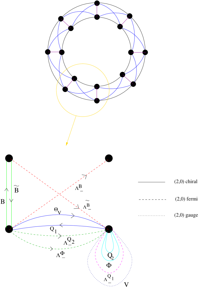
Figure 2: “Mating Moose”: Quiver diagram for intersecting D3-branes at a $\mathbb{C}^{2}/\mathbb{Z}_{k}$ orbifold (with $k$=8). The nodes of the inner and outer circle are associated with the $SU(N^{\prime})^{k}$ and $SU(N)^{k}$ gauge groups respectively. The parts which have not been drawn in the detailed “close-up” are easily inferred from the $\mathbb{Z}_{k}$ symmetry and by swapping D3 degrees of freedom with D$3^{\prime}$ degrees of freedom.

We do not need the full action of the $(4,0)$ quiver theory. For now we just give the the $(2,0)$ term analogous to a superpotential, which will be all that we require for most purposes. Superpotentials of $(2,0)$ theories have the generic structure

$$W=\int d\theta^{+}\sum_{a}\Lambda^{a}J_{a}(\Phi_{i})|_{\theta^{+}=0}\,,$$ (3.9)

where $J_{a}(\Phi_{i})$ is a holomorphic function of the chiral superfields satisfying a certain constraint (see the appendix). For the D3-D3 intersection at a $\mathbb{C}^{2}/\mathbb{Z}_{k}$ orbifold, this term descends from the superpotential of the D3-D3 intersection in flat space which is presented in $(2,0)$ superspace in the appendix. Upon projecting out the degrees of freedom which are not invariant under the orbifold (3.2), one obtains the $(2,0)$ superpotential

$$W=W_{\rm D3}+W_{\rm D3^{\prime}}+W_{\rm D3-D3^{\prime}}\,,$$ (3.10)

where

$$W_{\rm D3}=\int d^{2}xd\theta^{+}{\rm tr}_{N\times N} \left(g\Lambda^{\Phi}_{j,j+1}(Q^{2}_{j+1}Q^{1}_{j+1,j}\,-\,Q^{1}_{j+1,j}Q^{2}_{j})\right.$$ (3.11)

$$+ \,\Lambda^{Q^{1}}_{j}[\partial_{\bar{x}}+g\Phi_{j},Q^{2}_{j}]$$

$$+ \,\left.\left.\Lambda^{Q^{2}}_{j,j+1}(-\partial_{\bar{x}}Q^{1}_{j+1,j}-gQ^{1}_{j+1,j}\Phi_{j}+g\Phi_{j+1}Q^{1}_{j+1,j})\right)\right|_{\bar{\theta}^{+}=0}\,,$$

$$W_{\rm D3^{\prime}}=\int d^{2}yd\theta^{+}{\rm tr}_{N^{\prime}\times N^{\prime}} \left(g\Lambda^{\Upsilon}_{j,j+1}(S^{2}_{j+1}S^{1}_{j+1,j}\,-\,S^{1}_{j+1,j}S^{2}_{j})\right.$$ (3.12)

$$+ \,\Lambda^{S^{1}}_{j}[\partial_{\bar{x}}+g\Upsilon_{j},S^{2}_{j}]$$

$$+ \,\left.\left.\Lambda^{S^{2}}_{j,j+1}(-\partial_{\bar{x}}S^{1}_{j+1,j}-gS^{1}_{j+1,j}\Upsilon_{j}+g\Upsilon_{j+1}S^{1}_{j+1,j})\right)\right|_{\bar{\theta}^{+}=0}\,,$$

$$W_{\rm D3-D3^{\prime}}=g\int d\theta^{+}{\rm tr}_{N\times N} \left(\Lambda^{B}_{j,j+1}(\tilde{B}_{j+1}Q^{1}_{j,j+1}-S^{1}_{j+1,j}\tilde{B}_{j})+\Lambda^{Q^{1}}_{j}B_{j}\tilde{B}_{j}\right)$$ (3.13)

$$+{\rm tr}_{N^{\prime}\times N^{\prime}} \left.\left(\Lambda^{\tilde{B}}_{j,j+1}(Q^{1}_{j+1,j}B_{j}-B_{j+1}S^{1}_{j+1,j})-\Lambda^{S^{1}}_{j}\tilde{B}_{j}B_{j}\right)\right|_{\bar{\theta}^{+}=0}\,.$$

In order to see that this theory has indeed $(4,0)$ supersymmetry, we record the basic structure of the $(4,0)$ multiplets which appear. These are as follows:

i) $(4,0)$ hypermultiplets composed of two $(2,0)$ chiral multiplets: There are five multiplets of this type containing the pairs $(B,\tilde{B}),(\Phi,Q_{2}),(\Theta_{V},Q_{1}),(\Upsilon,S_{2})$ and $(\Theta_{\cal V},S_{1})$.

ii) $(4,0)$ vector multiplets composed of one $(2,0)$ vector multiplet and one $(2,0)$ fermi multiplet: There are two multiplets of this type containing the pairs $(V,\Lambda^{Q_{1}})$ and $({\cal V},\Lambda^{S_{1}})$.

iii) $(4,0)$ Fermi multiplets composed of one $(2,0)$ Fermi multiplet: There are six multiplets of this type corresponding to the $(2,0)$ fermi multiplets $\Lambda^{B},\Lambda^{\tilde{B}},\Lambda^{\Phi},\Lambda^{Q_{2}},\Lambda^{\Upsilon}$ and $\Lambda^{S_{2}}$.

The transformation properties under the $(4,0)$ $SU(2)_{L}$ R-symmetry are readily obtained from table 1 on page 1. Note that the $SU(2)_{L}$ R-symmetry acts on the degrees of freedom of either the inner or outer ring of the quiver diagram as the $SU(2)$ R-symmetry of the associated ${\cal N}=2,d=4$ theory.

In the following section, we shall make use of this superpotential to discuss the (de)construction of the M5-M5 intersection.

4 (De)constructing the M5-M5 intersection

The inner and outer circle of the quiver diagram in figure 2 are each separately equivalent to the quiver diagram of figure 1, which (de)constructs the $(2,0)$ theory upon taking the appropriate large $k$ limit [5]. The new twist here is that there are degrees of freedom connecting the inner and outer rings. These are localized at the intersection of the D3-branes, and it is natural to expect that in the large $k$ limit, these correspond to the tensionless strings localized at the intersection of M5-branes. One reason to expect this follows from a trivial extension of an argument given in [5] based on the IIB string theory embedding. The basic idea is that in the $k\rightarrow\infty$ limit, the $\mathbb{C}^{2}/\mathbb{Z}_{k}$ orbifold appears as a flat $S^{1}\times\mathbb{R}^{3}$ geometry to D3-brane sufficiently far away from the orbifold point (or sufficiently far out on the Higgs branch). For intersecting D3-branes, T-dualizing and lifting to M-theory on this space gives rise to intersecting M5-branes wrapping a torus of fixed dimensions. The strings stretched between the orthogonal D3-branes then become membranes stretched between M5-branes, as shown in figure 3. In the following, we shall focus on the field theoretic origins of the tensionless strings at the intersection.

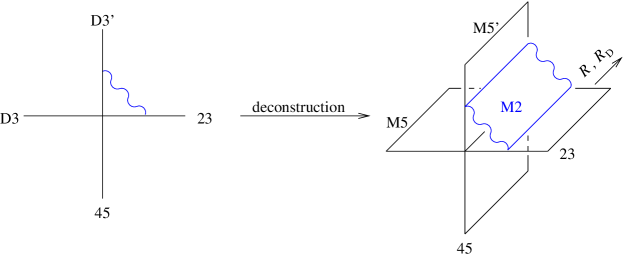
Figure 3: (De)construction of two extra dimensions along the torus with radii $R$ and $R_{D}$. The common directions $x^{0}$ and $x^{1}$ as well as the four orbifold directions are surpressed.

4.1 (De)constructing the $(2,0)$ theory

Before discussing the strings localized at the intersection, we shall briefly review the field theoretic arguments behind the (de)construction of the six-dimensional $(2,0)$ theory discovered in [5]. The quiver diagram of the deconstructed theory is that of figure 1, which describes a superconformal ${\cal N}=2,d=4$ gauge theory with gauge group $SU(N)^{k}$. The hypermultiplets described by the double lines stretched between adjacent nodes contain two complex scalars in bifundamental representations. The quiver diagram can be viewed as a discretization of an extra circular spatial dimension if one takes all the bifundamental scalars to have the same non-zero expectation value. At this point on the Higgs branch the gauge symmetry is broken from $SU(N)^{k}$ to the diagonal $SU(N)$.

To make closer contact with our work, we show how the extra dimensions arise from the ${\cal N}=2,d=4$ theory using the language of two-dimensional $(2,0)$ superspace. Consider the term $W_{\rm D3}$ in the superpotential (3.10), which involves only fields on the outer ring of the quiver diagram. Deconstructing the six-dimensional $(2,0)$ theory involves going to a particular point in the Higgs branch of the ${\cal N}=2,d=4$ theory described by the outer ring. At this point $\langle q^{1}_{j+1,j}\rangle=vI$ for all $j$, where $v$ is real and $q^{1}$ is the scalar component of $Q^{1}$. One then has an effective superpotential with the quadratic terms

$$W_{\rm D3}=\int d^{2}xd\theta^{+}{\rm tr}_{N\times N} \left(gv\Lambda^{\Phi}_{j,j+1}(Q^{2}_{j+1}-Q^{2}_{j})+gv\Lambda^{Q^{2}}_{j,j+1}(\Phi_{j+1}-\Phi_{j})\right.$$

$$\,+\left.\left.\Lambda^{Q^{1}}_{j}\partial_{\bar{x}}Q^{2}_{j}-\Lambda^{Q^{2}}_{j,j+1}\partial_{\bar{x}}{\cal P}_{j+1,j}\right)\right|_{\theta^{+}=0}\,,$$ (4.1)

where ${\cal P}_{j+1,j}=v-Q^{1}_{j+1,j}$. The first and second terms in (4.1) can be viewed as kinetic terms on a lattice with $k$ sites and lattice spacing $a=1/{gv}$. The bosonic kinetic terms arise upon integrating out auxiliary fields. From a two-dimensional point of view, the first two terms in (4.1) give rise to a mass matrix with eigenvalues

$$M^{2}=(gv)^{2}|e^{2\pi in/k}-1|^{2}\,.$$ (4.2)

For sufficiently large $k$, this becomes a Kaluza-Klein spectrum $M^{2}=(n/R)^{2}$ with $R=\frac{k}{gv}$.

Yet another compact dimension is generated due to the S-duality of the ${\cal N}=2,d=4$ gauge theory. Under S-duality $g\rightarrow k/g$ and one therefore expects a spectrum of S-dual states with masses

$$M_{D}^{2}=\left(\frac{kv}{g}\right)^{2}|e^{2\pi in/k}-1|^{2}\,.$$ (4.3)

For large $k$ and fixed $n$ there is a Kaluza-Klein spectrum on an S-dual circle of radius

$$2\pi R_{D}=\frac{g}{v}\,.$$ (4.4)

The continuum limit is obtained by taking $k\rightarrow\infty$ with $R,R_{D}$ fixed. This requires that one goes to strong coupling $g\sim\sqrt{k}$ and that one goes far out onto the Higgs branch $v\sim\sqrt{k}$.

4.1.1 A note on stability of the spectrum

The existence of the continuum limit is actually more subtle than the previous discussion suggests since it includes a strong coupling limit. Although string theory indicates the limit should exist, a field theoretical argument would have to demonstrate the validity of the semiclassical spectrum (4.2) at strong coupling, and $k\rightarrow\infty$ at fixed $n$. Strictly speaking, this spectrum is not a BPS mass formula for finite $k$, since the “charge” $n$ is defined modulo $k$ and is therefore not a central charge. Assuming the existence of a continuum limit with enhanced supersymmetry, the spectrum is BPS with respect to this enhanced supersymmetry. In [6], an argument that the supersymmetry enhancement is robust at low energies was given by studying the Seiberg-Witten curve of the ${\cal N}=2,d=4$ quiver gauge theory.

A further argument in favor of the stability of the spectrum at finite $k$ is as follows. Although the first two terms in (4.1) are lattice kinetic terms, they appear in the $(2,0)$ superpotential, which has a holomorphic structure and is protected against radiative corrections. If we were to work with four-dimensional ${\cal N}=1$ superspace, we would also find that the lattice kinetic terms arise in part from the effective superpotential on the Higgs branch. In ${\cal N}=1,d=4$ superspace, the superpotential is

$$W=g\sum_{j=1}^{k}{\rm tr}\left(\Phi^{1}_{j}\,\Phi^{2}_{j,j+1}\Phi^{3}_{j+1,j}-\Phi^{1}_{j+1}\Phi^{3}_{j+1,j}\Phi^{2}_{j,j+1}\right)\,.$$ (4.5)

The effective superpotential corresponding to lattice kinetic terms is obtained on the Higgs branch by setting $\Phi^{2}_{j,j+1}=v+\Gamma^{2}_{j,j+1}$ and $\Phi^{3}_{j+1,j}=v+\Gamma^{3}_{j+1,j}$. The non-renormalization of the effective superpotential and terms related to it by supersymmetry is crucial for the stability of the spectrum (4.2) at large $g$, and to the existence of a continuum limit.

Note that the non-renormalization of the lattice kinetic terms is somewhat akin to the non-renormalization of the metric on the Higgs branch of four-dimensional ${\cal N}=2$ gauge theories. The latter non-renormalization can be argued, albeit in an unconventional way, by writing the action in two-dimensional $(2,2)$ superspace. The kinetic terms for the ${\cal N}=2,d=4$ hypermultiplet then arise partially from a $(2,2)$ superpotential of the form $\epsilon_{ij}Q_{i}\partial_{x}Q_{j}$ as in (2).

4.2 Strings at the intersection

Let us now consider the same $k\rightarrow\infty$ limit as above for the case in which there are orthogonal intersecting stacks of D3-branes. We will initially take the Higgs branch moduli for the ${\cal N}=2,d=4$ theories on the inner and outer ring of the quiver to be equal, such that $\langle s^{1}_{j+1,j}\rangle=vI_{N\times N}$ and $\langle q^{1}_{j+1,j}\rangle=vI_{N^{\prime}\times N^{\prime}}$. In this case, the inner and outer rings of the quiver can be expected to separately (de)construct the six-dimensional $(2,0)$ theory compactified on tori with the same dimensions. However one must also consider the strings stretching between the D3-branes, i.e. the “spokes” which connect the inner and outer rings of the quiver. We shall now argue that these (de)construct tensionless strings living at a four-dimensional intersection of the two six-dimensional world volumes.

The “spoke” degrees of freedom correspond to the $(2,0)$ chiral fields $B_{j},\tilde{B}_{j}$ and Fermi fields ${\Lambda^{B}}_{j,j+1},{\Lambda^{\tilde{B}}}_{j,j+1}$, which describe strings stretched between the two stacks of D3-branes. For $\langle s^{1}_{j+1,j}\rangle=vI_{N\times N}$ and $\langle q^{1}_{j+1,j}\rangle=vI_{N^{\prime}\times N^{\prime}}$, the quadratic part of the effective superpotential is

$$W_{\rm D3-D3^{\prime}}=gv\int d\theta^{+}{\rm tr}\left.\left[\Lambda^{\tilde{B}}_{j,j+1}(B_{j}-B_{j+1})+(\tilde{B}_{j+1}-\tilde{B}_{j})\Lambda^{B}_{j,j+1}\right]\right|_{\bar{\theta}^{+}=0}\,$$ (4.6)

which follows from (3.13). This can also be viewed as a lattice kinetic term. The same mass matrix arises for the fundamental degrees of freedom at the intersection as for those on the inner and outer circles of the quiver. Therefore these degrees of freedom also carry momentum in an extra dimension of radius $R$. The full theory is again expected to exhibit S-duality, based on its embedding in string theory. Thus there should also be S-dual degrees of freedom at the intersection which carry momentum in an extra dimension of radius $R_{D}$. Dyonic states carry momenta in both extra directions. The precise nature of degrees of freedom which are S-dual to the fundamental degrees of freedom $B,\Lambda^{B},\tilde{B}$ and $\Lambda^{\tilde{B}}$ remains an open question at the moment. However, assuming S-duality, the $k\rightarrow\infty$ limit generates two six-dimensional world volumes intersecting over four dimensions from a theory with two four-dimensional world volumes intersecting over two dimensions. Note that the inner and outer rings of the quiver do not see independent extra directions, since the apparent $\mathbb{Z}_{k}\times\mathbb{Z}_{k}$ symmetry is broken to $\mathbb{Z}_{k}$ by couplings to the degrees of freedom at the intersection.

The spoke degrees of freedom should be interpreted as tensionless strings wrapping the compact directions rather than particles. To see this, it is helpful to move the orthogonal stacks of D3-branes to different points in the orbifold. This corresponds to going to different points on the Higgs branches of theories described by the inner and outer rings of the quiver. For the inner ring the Higgs branch is characterized by vevs for $\sigma_{j,j+1}$ and $\bar{q}^{1}_{j,j+1}$ which form a doublet $Y_{j,j+1}$ of the $SU(2)_{L}$ R-symmetry. Similarly the Higgs branch for the outer ring is characterized by vevs for $\omega_{j,j+1}$ and $s^{1}_{j,j+1}$ which also form a doublet $Y^{\prime}_{j,j+1}$ of $SU(2)_{L}$. Consider the following point in the moduli space:

$$Y_{j,j+1}=\begin{pmatrix}v+\Delta/2\cr v+\Delta/2\end{pmatrix}\,,\qquad Y_{j,j+1}^{\prime}=\begin{pmatrix}v-\Delta/2\cr v-\Delta/2\end{pmatrix}\quad.$$ (4.7)

where $\Delta$ is real. One might worry that the extra dimensions seen by the degrees of freedom on the inner and outer rings of the quiver are no longer the same, since at different points on the Higgs branches, $\langle Y\rangle\neq\langle Y^{\prime}\rangle$, the radii are apparently different. However we shall keep $v\Delta$ fixed in the $k\rightarrow\infty$ limit with $v\sim\sqrt{k}$. In this limit the deconstructed radii are the same and correspond to the same spatial directions:

$$\lim_{k\rightarrow\infty}\frac{k}{g(v+\frac{\Delta}{2})}=\lim_{k\rightarrow\infty}\frac{k}{g(v-\frac{\Delta}{2})}=R\,,$$

$$\lim_{k\rightarrow\infty}\frac{g}{v+\frac{\Delta}{2}}=\lim_{k\rightarrow\infty}\frac{g}{v-\frac{\Delta}{2}}=R_{D}\,.$$ (4.8)

At the point in moduli space given in (4.7), the quadratic part of the effective $(2,0)$ superpotential is

$$W =gv\int d\theta^{+}{\rm tr}\left.\left[B_{j}({\Lambda^{\tilde{B}}_{-}}_{j,j+1}-{\Lambda^{\tilde{B}}_{-}}_{j-1,j})+{\Lambda^{B}_{-}}_{j,j+1}(\tilde{B}_{j+1}-\tilde{B}_{j})\right]\right|_{\bar{\theta}^{+}}$$

$$+\,g\Delta\int d\theta^{+}{\rm tr}\left.\left[B_{j}({\Lambda^{\tilde{B}}_{-}}_{j,j+1}+{\Lambda^{\tilde{B}}_{-}}_{j-1,j})+{\Lambda^{B}_{-}}_{j,j+1}(\tilde{B}_{j+1}+\tilde{B}_{j})\right]\right|_{\bar{\theta}^{+}}\,.$$ (4.9)

The second term in (4.9) is a mass term from the point of view of the lattice theory. For large $k$ and fixed $n$, diagonalizing the mass matrix for the fundamental spoke degrees of freedom gives

$$M^{2}=(g\Delta)^{2}+(n/R)^{2}\,,$$ (4.10)

where the integer $n$ is the lattice momentum obtained by Fourier transforming with respect to the index $j$ labeling points on the quiver. For simplicity let us set $n=0$, so that $m=g\Delta$. The S-dual modes then have $m_{D}=\frac{k}{g}\Delta$. Since $m/m_{D}=R_{D}/R$, the fundamental spoke degrees of freedom should be interpreted as strings wrapping the cycle of radius $R_{D}$, while their S-duals wrap the cycle of radius $R$ (see figure 4). The string tension is

$$T=\frac{m}{2\pi R_{D}}=\frac{m_{D}}{2\pi R}=v\Delta\,.$$ (4.11)

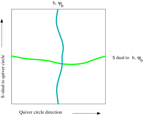
Figure 4: Strings localized at the intersection.

Note that the S-dual’s to the fundamental degrees of freedom at the intersection are strings wrapping the $S^{1}$ of the quiver diagram. Thus it is tempting to speculate that they can built from gauge invariant products of fundamental spoke degrees of freedom which wrap the quiver. An example of such an operator is ${\rm tr\,}\Lambda^{B}_{1,2}\Lambda^{\tilde{B}}_{2,3}\cdots\Lambda^{B}_{k-1,k}\Lambda^{\tilde{B}}_{k,1}$. On the other hand, one expects the S-dual operators to be solitons without an expression in terms of products of local operators, so this speculation is probably not quite correct.

4.3 String condensation and M5-branes on a holomorphic curve

When tensionless strings condense, the M5-M5 intersection is resolved to the holomorphic curve $xy=c$. This can be seen very explicitly from compactification on a torus. In this case the low energy theory is that of the D3-D3 intersection in flat space. In section 2 we showed that the Higgs branch of the corresponding $(4,4)$ dCFT can be interpreted as a resolution of the intersection to the holomorphic curve $xy=c$. The resolved intersection is also clearly captured by the $(4,0)$ dCFT. At the point in the moduli space for which extra dimensions are generated, the $(4,0)$ dCFT reduces to the $(4,4)$ dCFT at low energies. The potential is minimized by restricting to fields with values independent of the quiver index $j$ and satisfying equations equivalent to (2.8). The holomorphic curve $xy=c$ arises when the fields $B_{j}$ and $\tilde{B}_{j}$ get expectation values independent of $j$. These fields correspond to tensionless strings at the M5-M5 intersection.

4.4 Identifying R-symmetries and moduli

The M5-M5 intersection has ${\cal N}=2,d=4$ supersymmetry with $SU(2)\times U(1)$ R-symmetry. We would like to identify the corresponding charges in the $(4,0)$ defect conformal field theory.

For the $U(1)$ R-symmetry, the identification is as follows. This symmetry is manifest in both cases and corresponds to a simultaneous rotation of the $x$ and $y$ planes, which are transverse to one stack of parallel branes but not the orthogonal stack. In the $(4,0)$ dCFT, it is generated by $J_{23}-J_{45}$, and the associated charges can be readily obtained from table 1. Note that the other linear combination, $J_{23}+J_{45}$, is not an R-symmetry, and acts trivially on the degrees of freedom localized at the intersection.

We will now argue that the $SU(2)_{L}$ R-symmetry of the $(4,0)$ dCFT should be identified with the $SU(2)$ R-symmetry of the ${\cal N}=2,d=4$ theory of the M5-brane intersection. This matching is non trivial for the following reason. In order to generate the extra dimensions, it was neccessary to consider a point on the Higgs branch where the $SU(2)_{L}$ doublets $<Y>$ and $<Y^{\prime}>$ are non-zero, so that $SU(2)_{L}$ is spontaneously broken. On the other hand the $SU(2)$ R-symmetry of the M5-M5 intersection is only broken when M5-branes are transversely separated. Nevertheless, we shall find evidence that the identification makes sense. This suggests that when the M5-branes are not separated, the $SU(2)_{L}$ symmetry of the $(4,0)$ dCFT description is unbroken as far as the non-trivial dynamics is concerned.

There are three directions transverse to both stacks of M5-branes, corresponding to the moduli $\vec{X}$ and $\vec{X}^{\prime}$, which form a triplet under the $SU(2)$ R-symmetry. This R-symmetry is spontaneously broken if either $\vec{X}$ or $\vec{X}^{\prime}$ is non-zero. However if all the eigenvalues of $\vec{X}$ and $\vec{X}^{\prime}$ are the same, then the symmetry breaking is due only to trivial center of mass dynamics. The string tension $T=|\vec{X}-\vec{X}^{\prime}|$ vanishes at this point.

In the $(4,0)$ dCFT, the point in moduli space described by (4.7) corresponds to a string tension $T=v\Delta$. If we act with $SU(2)_{L}$, we obtain another point in moduli space which also deconstructs the same configuration of intersecting M5-branes. The string tension can be written in an $SU(2)_{L}$ invariant way as the expectation value of $|Y^{\dagger}\vec{\sigma}Y-{Y^{\prime}}^{\dagger}\vec{\sigma}Y^{\prime}|$ where $\vec{\sigma}$ are Pauli matrices. We have dropped the $j,j+1$ subscript as we only consider the zero momentum modes in the (de)constructed directions. On the other hand the string tension is related to the moduli of the M5-M5 intersection by $T=|\vec{X}-\vec{X}^{\prime}|$. This motivates the proposal

$$\vec{X}-\vec{X}^{\prime}\sim Y^{\dagger}\vec{\sigma}Y-{Y^{\prime}}^{\dagger}\vec{\sigma}Y^{\prime}\,.$$ (4.12)

Under $SU(2)_{L}$, $Y^{\dagger}\vec{\sigma}Y-{Y^{\prime}}^{\dagger}\vec{\sigma}Y^{\prime}$ transforms as a triplet, while $\vec{X}-\vec{X}^{\prime}$ transforms as triplet under $SU(2)$. This suggests that one should identify the $SU(2)_{L}$ R-symmetry of the $(4,0)$ theory with the $SU(2)$ R-symmetry of the M5-M5 intersection.

Thus far we have neglected a degree of freedom in the moduli space which also contributes to the string tension. There are four degrees of freedom in either $Y$ and or $Y^{\prime}$, while only three are characterized by $Y^{\dagger}\vec{\sigma}Y$ or ${Y^{\prime}}^{\dagger}\vec{\sigma}Y^{\prime}$. Note that $Y^{\dagger}\vec{\sigma}Y$ is invariant under $Y\rightarrow e^{i\theta}Y$, so the missing degree of freedom is an angle. The quantity $|Y^{\dagger}\vec{\sigma}Y-{Y^{\prime}}^{\dagger}\vec{\sigma}Y^{\prime}|=4vRe(\Delta)$ only gives the string tension for real $\Delta$. For complex $\Delta$ the string tension is easily seen to be $v|\Delta|$. The imaginary part of $\Delta$ corresponds to the additional angular degree of freedom. That the imaginary part is an angle is evident from the orbifold condition $(u,\bar{w})\sim\exp(2\pi i/k)(u,\bar{w})$ which for large $k$ gives $\Delta\sim\Delta+2\pi iv/k$. By viewing the quiver action as an action with only one extra discretized dimension (i.e. taking $R_{D}\rightarrow 0$ with fixed $R$), one discovers that the angular degree of freedom is a gauge connection in the compact discretized fifth direction. If the associated Wilson lines differ for the two intersecting branes, a mass term is generated for the degrees of freedom localized at the intersection. In terms of the six dimensional theories, this Wilson line may be interpreted as a Wilson surface corresponding to the holonomy of the mysterious non-abelian two-form on the torus.

4.5 A ’t Hooft anomaly

Although the deconstruction of the M5-M5 intersection involves a strong coupling limit, certain protected quantities such as ’t Hooft anomalies may be computed. We shall find a ’t Hooft anomaly in the $SU(2)_{L}$ R-current of the $(4,0)$ defect CFT. This means that there are Schwinger terms for correlators of the $SU(2)_{L}$ current which imply that the current is not conserved upon coupling to a background $SU(2)_{L}$ gauge field. For the M5-M5 intersection, this result suggests a ’t Hooft anomaly in the $SU(2)$ R-symmetry of the M5-M5 intersection due to tensionless strings.

Before discussing this anomaly, let us revisit the R-symmetry ’t Hooft anomaly which is known to arise for coincident M5-branes. The ’t Hooft anomaly in the $Spin(5)$ R-symmetry of the six-dimensional $(2,0)$ theory has been derived from anomaly cancellation considerations in M-theory [26], but never directly from a microscopic formulation of the $(2,0)$ theory, except in the abelian case [28]. The $Spin(5)$ R-symmetry can be viewed as part of the unbroken Lorentz symmetry for M-theory in the presence of flat parallel 5-branes. Since M-theory includes eleven-dimensional supergravity, this R-symmetry is actually gauged. The basic idea of [26] was to consider the long wavelength components of eleven-dimensional supergravity in the presence of a magnetic source, i.e. five-branes. The relevant terms in the supergravity action are

$$\int_{M_{11}}\,\left(C_{3}\wedge I_{8}^{inf}-\frac{2\pi}{6}C_{3}\wedge G_{4}\wedge G_{4}\right)\,,$$ (4.13)

where $G_{4}=dC_{3}$. In the presence of a magnetic source, such that

$$dG_{4}=Q_{5}\Pi_{i=6}^{10}\delta(x^{i})dx^{0}\wedge dx^{1}\cdots\wedge dx^{5}\,,$$ (4.14)

the term (4.13) is not invariant under diffeomorphisms of the normal bundle. Assuming that this anomaly is cancelled requires that the degrees of freedom on the M5-branes produce the opposite anomaly. In the decoupling limit, this anomaly becomes a ’t Hooft anomaly (or Schwinger term) for the global $Spin(5)$ R-symmetry of the $(2,0)$ theory.

Attempts to calculate this anomaly in the six-dimensional $(2,0)$ theory using its (de)constructed description [5] quickly run into a difficulty. The difficulty arises because the $Spin(5)$ R-symmetry of the $(2,0)$ theory is not manifest in the deconstructed description, which is a ${\cal N}=2,d=4$ superconformal Yang-Mills theory having only a $SU(2)\times U(1)$ R-symmetry. The full $Spin(5)$ symmetry can only arise in the continuum limit. Since the $SU(2)\times U(1)$ R-symmetry of the four-dimensional theory does not exhibit a ’t Hooft anomaly, one can not obtain information about the $Spin(5)$ anomaly without a detailed understanding of the enhancement of $SU(2)\times U(1)$ to $Spin(5)$ in the continuum limit. Note that even if it is possible to gauge a subgroup of a global symmetry without encountering an anomaly, the same may not be true for the full symmetry group.

In the case of intersecting M5-branes, we shall find that there is an additional anomaly which follows directly from the description in terms of the $(4,0)$ gauge theory. The $SU(2)$ R-symmetry of the intersecting five-branes corresponds to the $SU(2)_{L}$ R-symmetry of the $(4,0)$ gauge theory description, which exhibits a ’t Hooft anomaly. In a four-dimensional field theory, $SU(2)$ is free of ’t Hooft anomalies. Thus a contribution to a $SU(2)$ anomaly can only come from the two-dimensional degrees of freedom in the $(4,0)$ gauge theory. The only two-dimensional fermions charged under $SU(2)_{L}$ are contained in the $(4,0)$ hypermultiplets and have positive chirality. These make up a set of $k$ positive chirality doublets $(\Psi^{+}_{b,j},\bar{\Psi}^{+}_{\tilde{b},j})$ in the representation $(N,\bar{N}^{\prime})$ of $SU(N)_{j}\times SU(N^{\prime})_{j}$. Thus upon introducing a background $SU(2)_{L}$ gauge connection $\tilde{A}$, one finds the anomaly

$$D_{m}\frac{\delta S_{eff}(\tilde{A})}{\delta\tilde{A}_{m}^{a}(z)}=\frac{g^{2}}{4\pi}kNN^{\prime}\epsilon_{mn}\tilde{F}^{mn\,a}(z)\,,$$ (4.15)

where $m,n=0,1$. Some brief clarifying comments are in order about the meaning of the background $SU(2)_{L}$ gauge connection appearing in (4.15). This connection can be regarded as two connections on each of the intersecting world volumes of the dCFT, ${\cal A}_{\mu}(z,x)$ for $\mu=0,1,2,3$ and ${\cal A}^{\prime}_{\alpha}(z,y)$ for $\alpha=0,1,4,5$, subject to the constraint ${\cal A}_{0,1}(z,0)={\cal A}^{\prime}_{0,1}(z,0)\equiv\tilde{A}_{0,1}(z)$. In terms of a current equation, the anomaly for the dCFT coupled to an $SU(2)_{L}$ gauge connection is

$$\delta^{2}(y)D_{\mu}J^{\mu}(z,x)+\delta^{2}(x)D_{\alpha}J^{\prime\alpha}(z,y)+\delta^{2}(x)\delta^{2}(y) D_{m}{\cal J}^{m}(z)=$$

$$\delta^{2}(x)\delta^{2}(y)\frac{g}{4\pi}kNN^{\prime}\epsilon^{mn}{\tilde{F}}_{mn}(z)\,,$$ (4.16)

where $J$, $J^{\prime}$ and ${\cal J}$ depend on fields living on the D3-brane, the D3^′ brane, and the intersection respectively.

The question is now whether the anomaly (4.15) corresponds to a finite anomaly of the $SU(2)$ R-symmetry of the M5-M5 intersection in the $k\rightarrow\infty$ limit. If finite, the continuum limit should be interpreted as an anomaly arising from tensionless strings propagating in four dimensions. Note that while a local $SU(2)$ anomaly is not possible for a four-dimensional field theory, an $SU(2)$ anomaly of the M5-M5 intersection would be due to tensionless strings rather than local quantum fields! Unfortunately, we do not yet know how to obtain the continuum limit of (4.15), which can presumably be viewed as a sum of a discretized four-dimensional anomaly equation over the lattice sites.

An alternate way to derive the anomaly is to look for diffeomorphism anomalies of eleven-dimensional supergravity in the presence of magnetic sources due to intersecting M5-branes. The $SU(2)$ R-symmetry of the M5-M5 intersection is the Lorentz symmetry rotating the directions transverse to the intersecting five-branes. Thus in eleven-dimensional supergravity, the $SU(2)$ ’t Hooft anomaly becomes an anomaly in diffeomorphisms of the normal bundle. This should presumably be cancelled by an anomaly due to long-wavelength terms of the supergravity action in the presence of magnetic sources. We have not as yet been able to show this, however we will comment briefly on the contribution of the Chern-Simons terms (4.13) to the anomaly.

The first term in (4.13) is linear in $C^{3}$, while the second term is cubic. Only the cubic term can contribute to an anomaly localized at the five-brane intersection, due to mixed terms arising from the magnetic source

$$dG_{4}= N\Pi_{i=6,7,8,9,10}\,\delta(x^{i})\,dx^{0}\wedge dx^{1}\wedge dx^{2}\wedge dx^{3}\wedge dx^{4}\wedge dx^{5}$$

$$+ N^{\prime}\Pi_{i=4,5,8,9,10}\,\delta(x^{i})\,dx^{0}\wedge dx^{1}\wedge dx^{2}\wedge dx^{3}\wedge dx^{6}\wedge dx^{7}\,.$$ (4.17)

If the Chern-Simons term gives a non-zero anomaly, the coefficient will be proportional to $(N+N^{\prime})NN^{\prime}$. This apparently does not match the $N$ and $N^{\prime}$ dependence of (4.15). Perhaps the correct dependence somehow arises from correctly lifting (4.15) to a continuous four-dimensional version.

5 Conclusion and open questions

In this paper we have presented a formulation of intersecting M5-branes in terms of a limit of a $(4,0)$ defect conformal field theory. We hope that this will lead to an improved understanding of the low energy dynamics of M5-branes although, as for the (de)construction of parallel M5-branes [5], immediate progress is impeded by the fact that the continuum limit is also a strong coupling limit.

At the moment we only have control of a few some simple properties which are protected against radiative and non-perturbative corrections, such as the ’t Hooft anomaly in the $SU(2)$ R-current due to tensionless strings. This anomaly clearly deserves further study. In particular the contribution of M-theory Chern-Simons terms to the anomaly should be computed.

It would be interesting to try to generalize the construction here to more complicated intersections of branes in M-theory. Such generalizations might be of use in understanding the microscopic origins of black hole entropy.

It would also be very interesting to find field theoretic arguments in favor of the S-duality of the D3-D3 intersection, either in flat space or at a $\mathbb{C}^{2}/\mathbb{Z}_{k}$ orbifold. We have only assumed S-duality in this paper, based on the S-duality of the string theory background. A starting point would be to find solitons which are S-duals of degrees of freedom localized at the intersection. This is clearly very important if one wishes to have a better understanding of the degrees of freedom and dynamics of intersecting M5-branes.

Appendix A Gauge transformation properties

The gauge transformation properties under the residual gauge group $SU(N)^{k}\times SU(N^{\prime})^{k}$ in $(2,0)$ superspace are as follows:

$$\tilde{B}_{i} \rightarrow e^{-i\lambda^{\prime}_{i}}\tilde{B}_{i}e^{i\lambda_{i}},\quad\Lambda^{\tilde{B}}_{-,i}\rightarrow e^{-i\lambda^{\prime}_{i}}\Lambda^{\tilde{B}}_{-,i}e^{i\lambda_{i-1}},$$

$$B_{i} \rightarrow e^{-i\lambda_{i}}B_{i}e^{i\lambda^{\prime}_{i}},\quad\Lambda^{B}_{-,i}\rightarrow e^{-i\lambda_{i}}\Lambda^{B}_{-,i}e^{i\lambda^{\prime}_{i-1}}\,,$$

$$Q^{1}_{i} \rightarrow e^{-i\lambda_{i}}Q^{1}_{i}e^{i\lambda_{i+1}},\quad\Lambda_{-,i}^{Q^{1}}\rightarrow e^{-i\lambda_{i}}\Lambda_{-,i}^{Q^{1}}e^{i\lambda_{i}},$$ (A.1)

$$Q^{2}_{i} \rightarrow e^{-i\lambda_{i}}Q^{2}_{i}e^{i\lambda_{i}},\quad\Lambda_{-,i}^{Q^{2}}\rightarrow e^{-i\lambda_{i}}\Lambda_{-,i}^{Q^{2}}e^{i\lambda_{i+1}},$$

$$\Theta^{V}_{i} \rightarrow e^{-i\lambda_{i}}\Theta^{V}_{i}e^{i\lambda_{i-1}},\quad e^{V_{i}}\rightarrow e^{-i\lambda^{\dagger}_{i}}e^{V_{i}}e^{i\lambda_{i}},$$

$$S^{1}_{i} \rightarrow e^{-i\lambda^{\prime}_{i}}S^{1}_{i}e^{i\lambda^{\prime}_{i+1}},\quad\Lambda_{-,i}^{S^{1}}\rightarrow e^{-i\lambda^{\prime}_{i}}\Lambda_{-,i}^{S^{1}}e^{i\lambda^{\prime}_{i}},$$

$$S^{2}_{i} \rightarrow e^{-i\lambda^{\prime}_{i}}S^{2}_{i}e^{i\lambda^{\prime}_{i}},\quad\Lambda_{-,i}^{S^{2}}\rightarrow e^{-i\lambda^{\prime}_{i}}\Lambda_{-,i}^{S^{2}}e^{i\lambda^{\prime}_{i+1}},$$

$$\Theta^{\cal V}_{i} \rightarrow e^{-i\lambda^{\prime}_{i}}\Theta^{\cal V}_{i}e^{i\lambda^{\prime}_{i-1}},\quad e^{{\cal V}_{i}}\rightarrow e^{-i{\lambda^{\prime}}^{\dagger}_{i}}e^{{\cal V}_{i}}e^{i\lambda^{\prime}_{i}}\,,$$

where $i=1,\dots k$. These gauge transformations lead to the quiver diagram of figure 2. Strictly speaking, the transformation laws for the Fermi multiplets hold only at $\bar{\theta}^{+}=0$. Note that Fermi multiplets in superpotentials act effectively as chiral multiplets.

Appendix B Superpotential in manifest $(2,0)$ language

The conformal field theory corresponding to the D3-D3 intersection placed at an orbifold singularity is $(4,0)$ supersymmetric. For an adequate formulation of the parent defect theory in flat space, we use $(2,0)$ superspace. For the purposes of this paper it is sufficient to give the superpotential of the parent theory, which we now express in terms of $(2,0)$ superfields. Writing the full $(4,4)$ supersymmetric action (2) - (2) in $(2,0)$ superspace is straightforward, but we do not give the result here.

We decompose the $(2,2)$ defect multiplets $\bf B$ and $\bf\tilde{B}$ as well as the ambient multiplets $\bf Q_{1}$, $\bf Q_{2}$, $\bf\Phi$, and $\bf V$ under (2,0) supersymmetry. The reduction of $(2,2)$ multiplets to $(2,0)$ multiplets is discussed in [39, 40].

In general, a $(2,2)$ chiral multiplet $\bf\Phi$ reduces to two $(2,0)$ multiplets, a chiral multiplet $\Phi$ and a Fermi multiplet $\Lambda_{-}$, according to

$$\mathbf{\Phi}(y,\theta^{\pm})=\Phi(y,\theta^{+},\bar{\theta}^{+})|_{\bar{\theta}^{+}=0}+\sqrt{2}\theta^{-}\Lambda_{-}(y,\theta^{+},\bar{\theta}^{+})|_{\bar{\theta}^{+}=0}\,$$ (B.1)

with $y^{M}=x^{M}+i\theta^{+}\bar{\theta}^{+}+(-1)^{M}i\theta^{-}\bar{\theta}^{-}$ ($M=0,1$). The chiral $(2,0)$ multiplet satisfies ${\cal\bar{D}}_{+}\Phi=0$ and can be expanded as

$$\Phi=\phi+\sqrt{2}\theta^{+}\lambda_{+}-i\theta^{+}\bar{\theta}^{+}(D_{0}+D_{1})\phi\,$$ (B.2)

with covariant derivatives $D_{M}=\partial_{M}+\frac{ig}{2}v_{M}$. The Fermi multiplet expansion is given by

$$\Lambda_{-}=\psi_{-}+\sqrt{2}\theta^{+}F-i\theta^{+}\bar{\theta}^{+}(D_{0}+D_{1})\psi_{-}-\sqrt{2}\bar{\theta}^{+}E\,.$$ (B.3)

$\Lambda_{-}$ satisfies ${\cal\bar{D}}_{+}\Lambda_{-}=\sqrt{2}E$. In the reduction of the above $(2,2)$ chiral superfield $\bf\Phi$, the function $E$ is $E=i\sqrt{2}T^{a}\Theta^{a}_{V}\Phi$, where $T_{a}$ are the generators of the gauge group. Here $\Theta_{V}$ is another chiral superfield defined by

$$\Theta_{V}\equiv\mathbf{\Sigma}|_{\theta^{-}=\bar{\theta}^{-}=0}=\sigma+i\theta^{+}\bar{\lambda}_{+}-i\theta^{+}\bar{\theta}^{+}(D_{0}+D_{1})\sigma\,,$$ (B.4)

where $\bf\Sigma$ is the gauge invariant field strength of the (2,2) gauge multiplet $\bf V$.

We can now write the superpotential $W^{\rm par}=W^{\rm par}_{\rm D3}+W^{\rm par}_{\rm D3}+W^{\rm par}_{\rm D3-D3^{\prime}}$ of the parent theory, by substituting the following expansions into the action (2)-(2),

$$\mathbf{Q}_{i} =(Q_{i}+\sqrt{2}\theta^{-}\Lambda^{Q_{i}}_{-})|_{\bar{\theta}^{+}=0}\,,\qquad\mathbf{B}=(B+\sqrt{2}\theta^{-}\Lambda^{B}_{-})|_{\bar{\theta}^{+}=0}\,,$$ (B.5)

$$\mathbf{\Phi} =(\Phi+\sqrt{2}\theta^{-}\Lambda^{\Phi}_{-})|_{\bar{\theta}^{+}=0}\,,\qquad\,\,\,\,\mathbf{\tilde{B}}=(\tilde{B}+\sqrt{2}\theta^{-}\Lambda^{\tilde{B}}_{-})|_{\bar{\theta}^{+}=0}\,.$$ (B.6)

For the superpotential $W^{\rm par}_{\rm D3}$ associated with one stack of D3-branes, we find

$$W^{\rm par}_{\rm D3}= \int d^{2}xd^{2}\theta\,\epsilon_{ij}{\rm\,tr\,}\mathbf{Q}_{i}[\partial_{\bar{x}}+g\mathbf{\Phi},\mathbf{Q}_{j}]+c.c$$ (B.7)

$$= \int d^{2}xd\theta^{+}{\rm tr\!}\left.\left(\Lambda_{-}^{Q_{1}}[\partial_{\bar{x}}+g\Phi,Q_{2}]-\Lambda_{-}^{Q_{2}}[\partial_{\bar{x}}+g\Phi,Q_{1}]+g\Lambda_{-}^{\Phi}[Q_{2},Q_{1}]\right)\right|_{\bar{\theta}^{+}=0}\!+\!c.c.$$

A similar expression holds for $W^{\rm par}_{\rm D3^{\prime}}$, while the defect action has the $(2,0)$ superpotential

$$W^{\rm par}_{\rm D3-D3^{\prime}}=\frac{ig}{2}\int d\theta^{+}{\rm\,tr} \left(B\tilde{B}\Lambda_{-}^{Q_{1}}+\Lambda^{B}_{-}\tilde{B}Q_{1}+B\Lambda^{\tilde{B}}_{-}Q_{1}\right.$$

$$-\tilde{B}B\Lambda_{-}^{S_{1}}-\Lambda^{\tilde{B}}_{-}BS_{1}-\tilde{B}\Lambda^{B}_{-}S_{1}\left.\big{)}\right|_{\bar{\theta}^{+}=0}+c.c.$$ (B.8)

The parent superpotential $W^{\rm par}$ leads to the superpotential (3.10) under the orbifold projection.

References

- [1] E. Witten, “Some comments on string dynamics,” [arXiv:hep-th/9507121].
- [2] A. Strominger, “Open p-branes,” Phys. Lett. B 383, 44 (1996) [arXiv:hep-th/9512059].
- [3] X. Bekaert, M. Henneaux and A. Sévrin, “Chiral forms and their deformations,” Commun. Math. Phys. 224, 683 (2001) [arXiv:hep-th/0004049].
- [4] O. Aharony, M. Berkooz, S. Kachru, N. Seiberg and E. Silverstein, “Matrix description of interacting theories in six dimensions,” Adv. Theor. Math. Phys. 1, 148 (1998) [arXiv:hep-th/9707079].
- [5] N. Arkani-Hamed, A. G. Cohen, D. B. Kaplan, A. Karch and L. Motl, “Deconstructing (2,0) and little string theories,” [arXiv:hep-th/0110146].
- [6] C. Csaki, J. Erlich, J. Terning, “Seiberg-Witten Description of the Deconstructed 6D (0,2) Theory,” [arXiv:hep-th/0208095].
- [7] N. Arkani-Hamed, A. G. Cohen and H. Georgi, “(De)constructing dimensions,” Phys. Rev. Lett. 86 (2001) 4757 [arXiv:hep-th/0104005].
- [8] C. Csaki, J. Erlich, C. Grojean and G. D. Kribs, “4D constructions of supersymmetric extra dimensions and gaugino mediation,” Phys. Rev. D 65 (2002) 015003 [arXiv:hep-ph/0106044].
- [9] A. Hanany and I. R. Klebanov, “On tensionless strings in 3+1 dimensions,” Nucl. Phys. B 482, 105 (1996) [arXiv:hep-th/9606136].
- [10] S. Kachru, Y. Oz and Z. Yin, “Matrix description of intersecting M5 branes,” JHEP 9811, 004 (1998) [arXiv:hep-th/9803050].
- [11] S. Sethi, “The matrix formulation of type IIB five-branes,” Nucl. Phys. B 523, 158 (1998) [arXiv:hep-th/9710005].
- [12] O. J. Ganor and S. Sethi, “New perspectives on Yang-Mills theories with sixteen supersymmetries,” JHEP 9801 (1998) 007 [arXiv:hep-th/9712071].
- [13] A. Kapustin and S. Sethi, “The Higgs branch of impurity theories,” Adv. Theor. Math. Phys. 2, 571 (1998) [arXiv:hep-th/9804027].
- [14] A. Karch and L. Randall, “Locally localized gravity,” JHEP 0105, 008 (2001) [arXiv:hep-th/0011156].
- [15] A. Karch and L. Randall, “Open and closed string interpretation of SUSY CFT’s on branes with boundaries,” JHEP 0106 (2001) 063 [arXiv:hep-th/0105132].
- [16] A. Karch and L. Randall, “Localized gravity in string theory,” Phys. Rev. Lett. 87, 061601 (2001) [arXiv:hep-th/0105108].
- [17] O. DeWolfe, D.Z. Freedman and H. Ooguri, “Holography and Defect Conformal Field Theories,” [arXiv:hep-th/0111135].
- [18] J. Erdmenger, Z. Guralnik and I. Kirsch, “Four-dimensional superconformal theories with interacting boundaries or defects,” Phys. Rev. D 66, 025020 (2002) [arXiv:hep-th/0203020].
- [19] P. Lee and J. w. Park, “Open strings in PP-wave background from defect conformal field theory,” [arXiv:hep-th/0203257].
- [20] K. Skenderis and M. Taylor, “Branes in AdS and pp-wave spacetimes,” JHEP 0206, 025 (2002) [arXiv:hep-th/0204054].
- [21] C. Bachas, J. de Boer, R. Dijkgraaf and H. Ooguri, “Permeable conformal walls and holography,” JHEP 0206, 027 (2002) [arXiv:hep-th/0111210].
- [22] T. Quella and V. Schomerus, “Symmetry breaking boundary states and defect lines,” JHEP 0206, 028 (2002) [arXiv:hep-th/0203161].
- [23] D. Mateos, S. Ng and P. K. Townsend, “Supersymmetric defect expansion in CFT from AdS supertubes,” JHEP 0207, 048 (2002) [arXiv:hep-th/0207136].
- [24] N.R. Constable, J. Erdmenger, Z. Guralnik and I. Kirsch, “Intersecting D3-branes and Holography,” [arXiv:hep-th/0211222].
- [25] D. Freed, J. A. Harvey, R. Minasian and G. W. Moore, “Gravitational anomaly cancellation for M-theory fivebranes,” Adv. Theor. Math. Phys. 2, 601 (1998) [arXiv:hep-th/9803205].
- [26] J. A. Harvey, R. Minasian and G. W. Moore, “Non-abelian tensor-multiplet anomalies,” JHEP 9809, 004 (1998) [arXiv:hep-th/9808060].
- [27] K. A. Intriligator, “Anomaly matching and a Hopf-Wess-Zumino term in 6d, N = (2,0) field theories,” Nucl. Phys. B 581, 257 (2000) [arXiv:hep-th/0001205].
- [28] E. Witten, “Five-brane effective action in M-theory,” J. Geom. Phys. 22, 103 (1997) [arXiv:hep-th/9610234].
- [29] L. Bonora and M. Rinaldi, “Normal bundles, Pfaffians and anomalies,” Nucl. Phys. B 578, 497 (2000) [arXiv:hep-th/9912214].
- [30] K. Lechner, P. A. Marchetti and M. Tonin, “Anomaly free effective action for the elementary M5-brane,” Phys. Lett. B 524, 199 (2002) [arXiv:hep-th/0107061].
- [31] A. Boyarsky, J. A. Harvey and O. Ruchayskiy, “A toy model of the M5-brane: Anomalies of monopole strings in five dimensions,” Annals Phys. 301, 1 (2002) [arXiv:hep-th/0203154].
- [32] M. Henningson and K. Skenderis, “The holographic Weyl anomaly,” JHEP 9807, 023 (1998) [arXiv:hep-th/9806087].
- [33] I. R. Klebanov and A. A. Tseytlin, “Entropy of Near-Extremal Black p-branes,” Nucl. Phys. B 475, 164 (1996) [arXiv:hep-th/9604089].
- [34] J. M. Maldacena, A. Strominger and E. Witten, “Black hole entropy in M-theory,” JHEP 9712, 002 (1997) [arXiv:hep-th/9711053].
- [35] N. Arkani-Hamed, Th. Gregoire, J. Wacker, “Higher dimensional supersymmetry in 4D superspace,” [arXiv:hep-th/0101233].
- [36] A. Hebecker, “5D Super Yang-Mills Theory in 4D Superspace, Superfield Brane Operators, and Applications to Orbifold GUTs,” [arXiv:hep-ph/0112230].
- [37] M. R. Douglas and G. W. Moore, “D-branes, Quivers, and ALE Instantons,” [arXiv:hep-th/9603167].
- [38] C. V. Johnson and R. C. Myers, “Aspects of type IIB theory on ALE spaces,” Phys. Rev. D 55, 6382 (1997) [arXiv:hep-th/9610140].
- [39] E. Witten, “Phases of N = 2 theories in two dimensions,” Nucl. Phys. B 403, 159 (1993) [arXiv:hep-th/9301042].
- [40] H. Garcia-Compean and A. M. Uranga, “Brane box realization of chiral gauge theories in two dimensions,” Nucl. Phys. B 539, 329 (1999) [arXiv:hep-th/9806177].
- [41] E. Witten, “An SU(2) Anomaly,” Phys. Lett. B 117, 324 (1982).