${\langle\varphi^{2}\rangle}$ for a scalar field in 2D black holes: a new uniform approximation

Abstract

We study nonconformal quantum scalar fields and averages of their local observables (such as ${\langle\varphi^{2}\rangle}^{\mbox{{ren}}}$ and $\langle T_{\mu\nu}\rangle^{\mbox{{ren}}}$) in a spacetime of a 2-dimensional black hole. In order to get an analytical approximation for these expressions the WKB approximation is often used. We demonstrate that at the horizon WKB approximation is violated for a nonconformal field, that is when the field mass or/and the parameter of non-minimal coupling do not vanish. We propose a new ”uniform approximation” which solves this problem. We use this approximation to obtain an improved analytical approximation for ${\langle\varphi^{2}\rangle}^{\mbox{{ren}}}$ in the 2-dimensional black hole geometry. We compare the obtained results with numerical calculations.

I Introduction

Calculation of local observables which characterize vacuum polarization in the gravitational field of a black hole is an old problem. Main motivation is connected with study of back reaction effects and constructing a self-consistent model of an evaporating black hole. A lot of information was obtained concerning properties of fluctuations ${\langle\varphi^{2}\rangle}^{\mbox{{ren}}}$ and vacuum stress-energy tensor $\langle T_{\mu\nu}\rangle^{\mbox{{ren}}}$ in Schwarzschild and Reissner-Nordstrom geometries. A superscript ren indicates that we are dealing with physical finite quantities after a renormalization has been done. Combination of numerical calculations [1, 2, 3, 4] and different analytical approximations [4, 5, 6, 7, 8, 9, 10] usually gives quite good results. Nevertheless, there still remains one problem. Analytical ‘approximation’ does not work in the vicinity of a black hole horizon if the spacetime is not Ricci flat and the quantum field is not conformally invariant. It gives logarithmically divergent result near the horizon in the Hartle-Hawking state, where one expects finite and smooth behavior. In four dimensions the general structure of this divergence reads (see e.g. [10])

$${\langle\varphi^{2}\rangle}^{\mbox{{ren}}}\sim a_{1}\,\ln(|g_{tt}|)\,,\hskip 14.22636pt\langle T_{\mu\nu}\rangle^{\mbox{{ren}}}\sim{\delta\int d^{4}v\,a_{2}\over\delta g^{\mu\nu}}\,\ln(|g_{tt}|)\,.$$ (1)

Analogously, in two dimensions it is

$${\langle\varphi^{2}\rangle}^{\mbox{{ren}}}\sim\,\ln(|g_{tt}|)\,,\hskip 14.22636pt\langle T_{\mu\nu}\rangle^{\mbox{{ren}}}\sim{\delta\int d^{4}v\,a_{1}\over\delta g^{\mu\nu}}\,\ln(|g_{tt}|)\,.$$ (2)

Here $a_{1}$ and $a_{2}$ are Schwinger-DeWitt coefficients. For massive scalar fields

$$a_{1} = [({1\over 6}-\xi)\,{\cal R}-\mu^{2}]\,,$$ (3)

$$a_{2} = {1\over 180}\left({\cal R}_{\mu\nu\alpha\beta}{\cal R}^{\mu\nu\alpha\beta}-{\cal R}_{\mu\nu}{\cal R}^{\mu\nu}+\Box{\cal R}\right)+{1\over 2}\left[({1\over 6}-\xi)\,{\cal R}-\mu^{2}\right]^{2}+{1\over 6}~{}({1\over 6}-\xi)\Box{\cal R}~{},$$ (4)

where $\mu$ is the mass of the field and $\xi$ is a parameter of non-minimal coupling with the curvature ${\cal R}$.

In order to obtain the analytical approximation Anderson, Hiscock, and Samuel [4] used WKB approximation for solutions of radial equations. Recently it was demonstrated that the breakdown of the analytical approximation (see discussion in Appendix A) is directly related to the breakdown of WKB approximation for so called zero modes, that is zero-frequency solutions [11, 12]. By using improved approximation for zero modes it is possible to correct the analytical approximation near the horizon and to make all calculated quantities finite. The concrete methods proposed in [11, 12] are based on the approximations to zero modes valid only in the vicinity of the horizon.

The aim of this paper is to develop a new uniform approximation scheme for calculations of zero-modes contribution to ${\langle\varphi^{2}\rangle}^{\mbox{{ren}}}$ and $\langle T_{\mu\nu}\rangle^{\mbox{{ren}}}$. Although the method is applicable in arbitrary dimensions, here, for simplicity, we restrict ourselves by studying ${\langle\varphi^{2}\rangle}^{\mbox{{ren}}}$ near two-dimensional black holes. We consider different interesting examples of 2D black hole metrics, and keep the mass of a scalar field $m$ and the parameter of non-minimal coupling $\xi$ arbitrary.

II Green’s function

Consider a massive quantum scalar field with an arbitrary curvature coupling in a spacetime of the 2-dimensional black hole. The metric of the static 2-dimensional black hole can be written in the form

$$dS^{2}=-Fdt^{2}+{dr^{2}\over F}\,,$$ (5)

where the function $F(r)$ should possess the following properties: (i) $F(r)$ vanishes at the horizon $r=r_{0}$ and (ii) $F(r)$ tends to $1$ at $r\to\infty$. It is convenient to rewrite the metric (5) in the dimensionless form as follows

$$ds^{2}=r_{0}^{-2}\,dS^{2}=-fd\tilde{t}^{2}+{dx^{2}\over f}\,,\hskip 28.45274ptf(x)=F(r)\,,$$ (6)

where $\tilde{t}=t/r_{0}$ and $x=(r-r_{0})/r_{0}$, so that the horizon is located at $x=0$. We shall also use the dimensionless mass $m=\mu r_{0}$ and curvature $R={\cal R}r_{0}^{2}$. By making Wick’s rotation $\tilde{t}\to i\tau$ in the metric (6) one gets the Euclidean metric of the form

$$ds_{E}^{2}=f\,d\tau^{2}+{dx^{2}\over f}\,.$$ (7)

It is well known that the property of periodicity of Green functions in the Euclidean time coordinate $\tau$ with the period $\beta=T^{-1}$, corresponds to quantum systems at finite temperature $T$. We consider the case of nonzero temperature $T$ and nonzero surface gravity $\kappa=f^{\prime}_{x}/2\big{|}_{x=0}$.

The Euclidean Green function $G_{E}(X,X^{\prime})$ is a solution of the equation

$$\left[\Box_{E}-m^{2}-\xi\,R\right]\,G_{E}(x,\tau;x^{\prime},\tau^{\prime})=-\delta(x,\tau;x^{\prime},\tau^{\prime})\,$$ (8)

which in the metric (7) has the following form

$$\left[f^{-1}{\partial^{2}\over\partial\tau^{2}}+{\partial\over\partial x}\left(f{\partial\over\partial x}\right)-m^{2}-\xi R\right]G_{E}(x,\tau;x^{\prime},\tau^{\prime})=-\delta(\tau-\tau^{\prime})\,\delta(x-x^{\prime})\,.$$ (9)

This equation allows a separation of variables, so that we can write

$$G_{E}(X,X^{\prime})=T{\cal G}_{0}(x,x^{\prime})+2T\sum_{n=1}^{\infty}\,\cos\left(\omega_{n}(\tau-\tau^{\prime})\right)\,{\cal G}_{n}(x,x^{\prime}),$$ (10)

where $\omega_{n}=2\pi nT$ and ${\cal G}_{n}$ are “radial” Green functions which are the solutions of the 1-dimensional problem

$$\left[{d\over dx}\left(f{d\over dx}\right)-\left(\frac{\omega_{n}^{2}}{f}+m^{2}+\xi R\right)\right]{\cal G}_{n}(x,x^{\prime})=-\delta(x-x^{\prime})\,.$$ (11)

The Green functions ${\cal G}_{n}$ can be written in the form

$${\cal G}_{n}(x,x^{\prime})=s^{(2)}_{n}(x^{<})s^{(1)}_{n}(x^{>})~{},$$ (12)

where $x^{>}=\max(x,x^{\prime})$ and $x^{<}=\min(x,x^{\prime})$. Here the radial modes $s^{(1)}_{n}$ and $s^{(2)}_{n}$ are two linear independent solutions of the homogeneous equation of motion

$$\left[{d\over dx}\left(f{d\over dx}\right)-\left({\omega_{n}^{2}\over f}+m^{2}+\xi R\right)\right]s(x)=0~{}.$$ (13)

We choose $s^{(1)}_{n}$ to be regular at infinity and $s^{(2)}_{n}$ to be regular at the horizon. The solutions $s^{(1)}_{n}$ and $s^{(2)}_{n}$ are normalized by the condition

$$s^{(1)}_{n}{ds^{(2)}_{n}\over dx}-s^{(2)}_{n}{ds^{(1)}_{n}\over dx}=-\frac{1}{f}~{}.$$ (14)

The coincidence limit of the Euclidean Green function gives the unrenormalized expression for $\langle\varphi^{2}\rangle$, which is ultraviolet divergent,

$$\langle\varphi^{2}(x)\rangle_{\rm unren}=G_{E}(x,\tau;x,\tau^{\prime})=T{\cal G}_{0}(x,x)+2T\sum_{n=1}^{\infty}\,\cos(\omega_{n}(\tau-\tau^{\prime}))\,{\cal G}_{n}(x,x).$$ (15)

(For convenience the points are split in time direction only, so $x^{\prime}=x$.) Subtraction of ultraviolet divergencies gives the renormalized ${\langle\varphi^{2}\rangle}$

$${\langle\varphi^{2}\rangle}_{\rm ren}=\lim_{\tau^{\prime}\to\tau}\left({\langle\varphi^{2}\rangle}_{\rm unren}-{\langle\varphi^{2}\rangle}_{\rm DS}\right)~{},$$ (16)

where ${\langle\varphi^{2}\rangle}_{\rm DS}$ is the DeWitt-Schwinger counterterm which in two dimensions has the following form

$${\langle\varphi^{2}\rangle}_{\rm DS}=-\frac{1}{4\pi}(\ln\frac{\mu^{2}\sigma}{2}+2C)~{}.$$ (17)

Here $\sigma$ is equal to one half the square of the distance between the points $x$ and $x^{\prime}$ along the shortest geodesic connecting them, $C$ is the Euler’s constant. For a massive fields the constant $\mu$ is equal to its mass. For a massless field it is an arbitrary mass scale parameter. A particular choice of the value of $\mu$ corresponds to a finite renormalization of the coefficients of terms in the gravitational Lagrangian.

The stress-energy tensor can be obtained by applying a certain differential operator to the Green function:

$$\langle T_{\mu\nu}\rangle=\lim_{X^{\prime}\to X}D_{\mu\nu}G_{E}(X,X^{\prime}).$$ (18)

In order to calculate ${\langle\varphi^{2}\rangle}$ and $\langle T_{\mu\nu}\rangle$ one needs to solve the radial equation of motion (13) and to find the radial Green functions ${\cal G}_{n}(x,x)$. In a general case it is impossible to find exact solutions of this equation, and so one oftes uses various approximate methods. In case the scalar field has a nonzero mass, one of the standard approaches is the WKB approximation. For example, recently Anderson, Hiscock and Samuel have derived the analytic approximation for ${\langle\varphi^{2}\rangle}$ and $\langle T_{\mu\nu}\rangle$ for a scalar field in the general static spherically symmetric spacetime using the WKB expansion for radial modes [4]. However, the serious obstacle for applying this method in black hole spacetimes is that the WKB approximation even in case $m>0$ breaks down at the horizon for low-frequency modes.

In the section IV we discuss this problem in more detail.

III Exactly solvable models

Let us consider the radial equation of motion (13). Let us introduce new variables

$$\frac{dx}{f(x)}=\frac{dy}{y},\quad s(x)=\frac{u(y)}{y^{1/2}},$$ (19)

and rewrite this equation in the form

$$\left[\frac{d^{2}}{dy^{2}}-\left(\frac{\omega_{n}^{2}-\frac{1}{4}}{y^{2}}+\frac{(m^{2}+\xi R){\cal F}}{y^{2}}\right)\right]u(y)=0~{}.$$ (20)

Here ${\cal F}(y)=f(x)$ and

$$R=-\frac{y^{2}{\cal F}^{\prime\prime}}{{\cal F}^{2}}-\frac{y{\cal F}^{\prime}}{{\cal F}^{2}}+\frac{y^{2}{\cal F}^{\prime 2}}{{\cal F}^{3}}~{}.$$ (21)

The prime means the derivative with respect to $y$.

First of all, let us discuss cases when the equation (20) can be solved exactly.

A Conformally invariant scalar field

Consider the 2d conformally invariant scalar field, i.e., assume $m=0$ and $\xi=0$. In this case the equation (20) takes the form

$$\left[\frac{d^{2}}{dy^{2}}-\frac{\omega_{n}^{2}-\frac{1}{4}}{y^{2}}\right]u=0.$$ (22)

Two independent solutions of this equation are

$$u_{n=0}^{(1)}=y^{1/2},\quad u_{n=0}^{(2)}=-y^{1/2}\,\ln y,$$ (23)

$$u_{n>0}^{(1)}=\frac{1}{\sqrt{2\omega_{n}}}\,y^{\omega_{n}+1/2},\quad u_{n>0}^{(2)}=\frac{1}{\sqrt{2\omega_{n}}}\,y^{-\omega_{n}+1/2}.$$ (24)

B 2D dilatonic black hole

Consider a scalar field in the 2D dilatonic black hole spacetime with (see [13])

$$f(x)=1-e^{-x}.$$ (25)

Using the coordinate $y$ we find

$${\cal F}(y)={y\over 1+y},$$ (26)

and

$$R=\frac{1}{1+y}~{}.$$ (27)

The equation (20) now reads

$$\frac{d^{2}u}{dy^{2}}-\left(\frac{\omega_{n}^{2}-\frac{1}{4}}{y^{2}}+\frac{m^{2}}{y(1+y)}+\frac{\xi}{y(1+y)^{2}}\right)u=0.$$ (28)

This equation can be solved in terms of hypergeometric functions [13]. Its two independent solutions are

$$u^{(1)}_{n} = y^{1/2-\Omega_{n}}\left(\frac{y}{1+y}\right)^{\omega_{n}+\Omega_{n}}F(a,b;2\omega_{n}+1;\frac{y}{1+y}),$$ (29)

$$u^{(2)}_{n} = y^{1/2-\Omega_{n}}\left(\frac{y}{1+y}\right)^{\omega_{n}+\Omega_{n}}F(a,b;2\Omega_{n}+1;\frac{1}{1+y}),$$ (30)

The Wronskian of these solutions is

$$W[u^{(1)}_{n},u^{(2)}_{n}]\equiv W_{n} = u^{(1)}_{n}\frac{du^{(2)}_{n}}{dy}-\frac{du^{(2)}_{n}}{dy}u^{(1)}_{n}=\frac{\Gamma(2\omega_{n}+1)\Gamma(2\Omega_{n}+1)}{\Gamma(a)\Gamma(b)},$$ (31)

where

$$\Omega_{n}=\sqrt{\omega_{n}^{2}+m^{2}},$$

and

$$a=\frac{1}{2}+\omega_{n}+\Omega_{n}+\frac{1}{2}\sqrt{1-4\xi}~{},\quad b=\frac{1}{2}+\omega_{n}+\Omega_{n}-\frac{1}{2}\sqrt{1-4\xi}~{}.$$

IV The WKB approximation for radial modes

In the cases when the analytical solution is not known WKB approximation is often used. Let us write the radial modes $s^{(1)}_{n}$ and $s^{(2)}_{n}$ in the WKB form

$$s^{(1)}_{n}(x)={1\over\sqrt{2\Omega(x)}}\exp\left(\int^{x}{\Omega(x^{\prime})\over f(x^{\prime})}dx^{\prime}\right),$$ (32)

$$s^{(2)}_{n}(x)={1\over\sqrt{2\Omega(x)}}\exp\left(-\int^{x}{\Omega(x^{\prime})\over f(x^{\prime})}dx^{\prime}\right),$$ (33)

where $\Omega(x)$ is a new unknown function. Note that these solutions are properly normalized to satisfy the condition (14). Substituting (32), (33) into (13) gives the equation for $\Omega(x)$:

$$\Omega^{2}=\omega_{n}^{2}+m^{2}f+\xi Rf+\frac{1}{2}{f^{2}\Omega^{\prime\prime}\over\Omega}+\frac{1}{2}{ff^{\prime}\Omega^{\prime}\over\Omega}-\frac{3}{4}{f^{2}\Omega^{\prime 2}\over\Omega^{2}}.$$ (34)

This equation can be solved iteratively with the zeroth-order solution chosen as

$$\Omega^{(0)}=\Omega_{0}=\left[\omega_{n}^{2}+m^{2}f\right]^{1/2}.$$ (35)

The first-order solution is

$$\Omega^{(1)}=\Omega_{0}+\Omega_{1}=\Omega_{0}+\frac{\xi Rf}{2\Omega_{0}}+\frac{1}{4}\frac{f^{2}\Omega_{0}^{\prime\prime}}{\Omega_{0}^{2}}+\frac{1}{4}\frac{ff^{\prime}\Omega_{0}^{\prime}}{\Omega_{0}^{2}}-\frac{3}{8}\frac{f^{2}{\Omega_{0}^{\prime}}^{2}}{\Omega_{0}^{3}}~{}.$$ (36)

Analogously, the $k$’th-order solution can be found

$$\Omega^{(k)}=\Omega_{0}+\Omega_{1}+\dots+\Omega_{k},$$ (37)

The WKB approximation is based on an assumption that

$$\Omega_{0}\gg\Omega_{1}\gg\dots\gg\Omega_{k}.$$ (38)

This ensures the convergence of series $\sum_{k=0}^{\infty}\Omega_{k}$ and allows one to break the series in order to construct an approximate solution for $\Omega$ of the form (37). Substituting $\Omega^{(k)}$ into (32), (33) gives the WKB approximation of $k$’th order for the radial modes $s^{(1,2)}_{n}$. By and substituting $s^{(1,2){\rm WKB}}_{n}$ into (40) and then into (15) one obtains the WKB approximation for $\langle\varphi^{2}\rangle_{\rm unren}$:

$$\langle\varphi^{2}(x)\rangle_{\rm unren,WKB}=T{\cal G}_{0}^{\rm WKB}(x,x)+2T\sum_{n=1}^{\infty}\,\cos(\omega_{n}(\tau-\tau^{\prime}))\,{\cal G}_{n}^{\rm WKB}(x,x),$$ (39)

with

$${\cal G}_{n}^{\rm WKB}(x,x)=s_{n}^{(1)\rm WKB}(x)s_{n}^{(2)\rm WKB}(x)~{}.$$ (40)

Let us discuss the validity of this approximation for zero-modes. i.e., when $n=0$. For $n=0$ one has $\Omega_{0}=mf^{1/2}$, i.e., $\Omega_{0}\sim f^{1/2}$. Then $\Omega_{1}\sim{f^{\prime}}^{2}f^{-1/2}$ (see Eq. (36)). Note that at the horizon the function $f$ vanishes while $f^{\prime}$ and $\kappa$ remain finite. Thus in the vicinity of the horizon $\Omega_{0}\ll\Omega_{1}$. Moreover, one can show that near the horizon inequalities $\Omega_{0}\ll\Omega_{1}\ll\dots\ll\Omega_{k}$ are fulfilled instead of (38). This means that the series $\sum_{k=0}^{\infty}\Omega_{k}$ diverges, and the WKB expansion breaks down. Thus, the WKB method can not be used for constructing ${\cal G}_{n=0}$ near the horizon.

V New uniform approximation for the radial modes

A General discussion

In this section we propose a new approximation which can be used instead of the WKB approximation.

We choose the time $T$ normalization so that the function ${\cal F}(y)$ tends to $1$ at $y\to\infty$. We assume also that the surface gravity does not vanish, so that ${\cal F}(y)\sim y$ at $y\to 0$. Let us write ${\cal F}(y)$ in the form

$${\cal F}(y)=\frac{y{\em h}(y)}{c+y}~{}.$$ (41)

Here $c>0$ is a positive constant, and ${\em h}(y)$ is a positive function depending on $c$ and having the asymptotics

$${\em h}(y)|_{y\to 0} = {\em h}_{0}+{\cal O}(y)~{},\hskip 56.9055pt{\em h}_{0}>0$$ (42)

$${\em h}(y)|_{y\to\infty} = 1+{\cal O}(y^{-1})~{}.$$ (43)

Note that such the representation explicitly reflects the asymptotical properties of ${\cal F}(y)$:

$${\cal F}(y)|_{y\to 0} = {\em h}_{0}c^{-1}y+{\cal O}(y^{2}),$$ (44)

$${\cal F}(y)|_{y\to\infty} = 1+{\cal O}(y^{-1}).$$ (45)

The expression (21) for the scalar curvature now reads

$$R=\frac{c}{(c+y){\em h}}-(c+y)\frac{{\em h}^{\prime}}{{\em h}^{2}}-y(c+y)\frac{{\em h}^{\prime\prime}}{{\em h}^{2}}+y(c+y)\frac{{{\em h}^{\prime}}^{2}}{{\em h}^{3}}~{}.$$ (46)

The equation (20) takes the form

$$\frac{d^{2}u}{dy^{2}}-\left(\frac{\omega_{n}^{2}-\frac{1}{4}}{y^{2}}+\frac{m^{2}{\em h}}{y(c+y)}+\frac{c\xi}{y(c+y)^{2}}+\xi V\right)u=0,$$ (47)

where

$$V(y)=-\frac{{\em h}^{\prime\prime}}{{\em h}}-\frac{{\em h}^{\prime}}{y{\em h}}+\frac{{\em h}^{\prime 2}}{{\em h}^{2}}.$$ (48)

In the special case $c=1$ and ${\em h}(y)\equiv 1$ we obtain the 2D dilatonic black hole with ${\cal F}(y)=y/(1+y)$ and $V=0$ (see Eqs. (26), (28)).

In a general case we will fix the constant $c$ by the algebraic condition

$${\em h}^{\prime}(0)=0,$$ (49)

in order that to guarantee the regular behavior of $V(y)$ near the horizon $y=0$. This condition shows that the function ${\em h}(y)$ near $y=0$ has the form:

$${\em h}(y)|_{y\to 0}={\em h}_{0}+{\cal O}(y^{2}).$$ (50)

We rewrite the equation (47) as

$$\frac{d^{2}u}{dy^{2}}-(U_{n}+\xi V)u=0,$$ (51)

where we denote

$$U_{n}(y)=\frac{\omega_{n}^{2}-\frac{1}{4}}{y^{2}}+\frac{m^{2}{\em h}}{y(c+y)}+\frac{c\xi}{y(c+y)^{2}}.$$ (52)

Let us compare two terms $U_{n}$ and $\xi V$. In case $\xi=0$ the term $\xi V$ disappears and the equation (51) takes the form

$$\frac{d^{2}u}{dy^{2}}-U_{n}u=0.$$ (53)

Now assume that $\xi$ does not vanish. Let us consider separately asymptotical regions near the horizon ($y\to 0$) and far from it ($y\to\infty$). Using the asymptotical form (50) for ${\em h}(y)$ we can find that near the horizon $V(y)={\cal O}(y^{0})$ and $U_{n}(y)={\cal O}(y^{-2})$, and hence in the limit $y\to 0$ the absolute value of the term $\xi V$ is much less than the one of $U_{n}$. Far from the horizon ${\em h}(y)=1+{\cal O}(y^{-1})$, then $V(y)={\cal O}(y^{-3})$ and $U_{n}(y)={\cal O}(y^{-2})$, and so we can again conclude that $|\xi V|\ll|U_{n}|$ in the limit $y\to\infty$.

In order to estimate values of the terms $\xi V$ and $U_{n}$ in the intermediate region $0<y<\infty$ we consider the particular configuration: two dimensional “Schwarzschild” black hole with

$$f(x)={x\over x+1}.$$ (54)

By using the relation ${dx/f(x)}={dy/y}$ we find

$$y=xe^{x}.$$ (55)

${\em h}$ as a function of $x$ can be obtained by comparing two representations, (41) and (54), for $f$:

$${\cal F}(y)={y{\em h}\over c+y}\,,$$

so that

$${\em h}\big{(}y(x)\big{)}={c+xe^{x}\over(x+1)e^{x}}.$$ (56)

The constant $c$ can be fixed by the condition (49), which gives $c=1/2$. $V$ and $U_{n}$ calculated for this metric are shown in the figures 1 and 2. In the figure 1 graphs for $y^{2}U_{n=0}$ are given for various values of $m$ and $\xi$. Note that in case $m<0.5$ the function $y^{2}U_{n=0}(y)$ is strictly negative, while for larger masses $m>0.5$ it can change sign, so that there is a point $y_{*}>0$ where $y_{*}^{2}U_{n=0}(y_{*})=0$. Hereafter we will assume that $m<0.5$. As for the $n>0$ modes one can easily see from Eq. (52) that the function $y^{2}U_{n>0}(y)$ is positive for arbitrary $m\geq 0$ and $\xi\geq 0$.

 

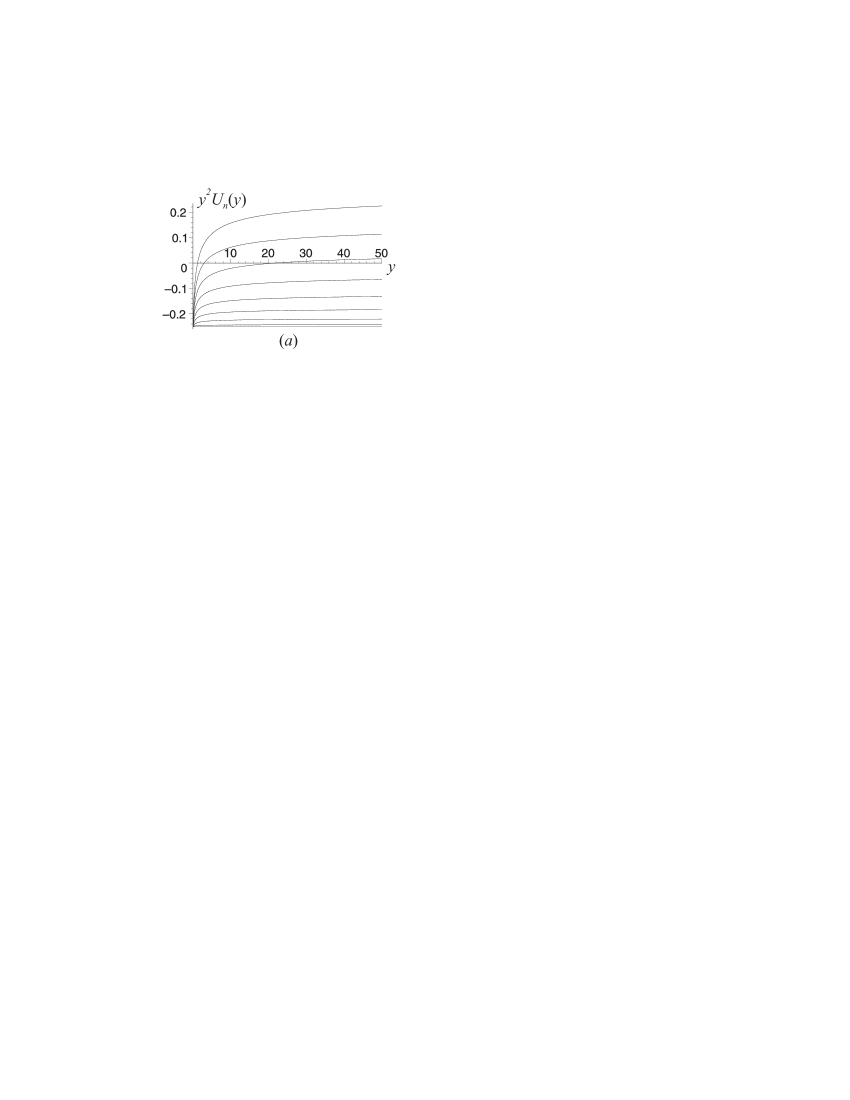
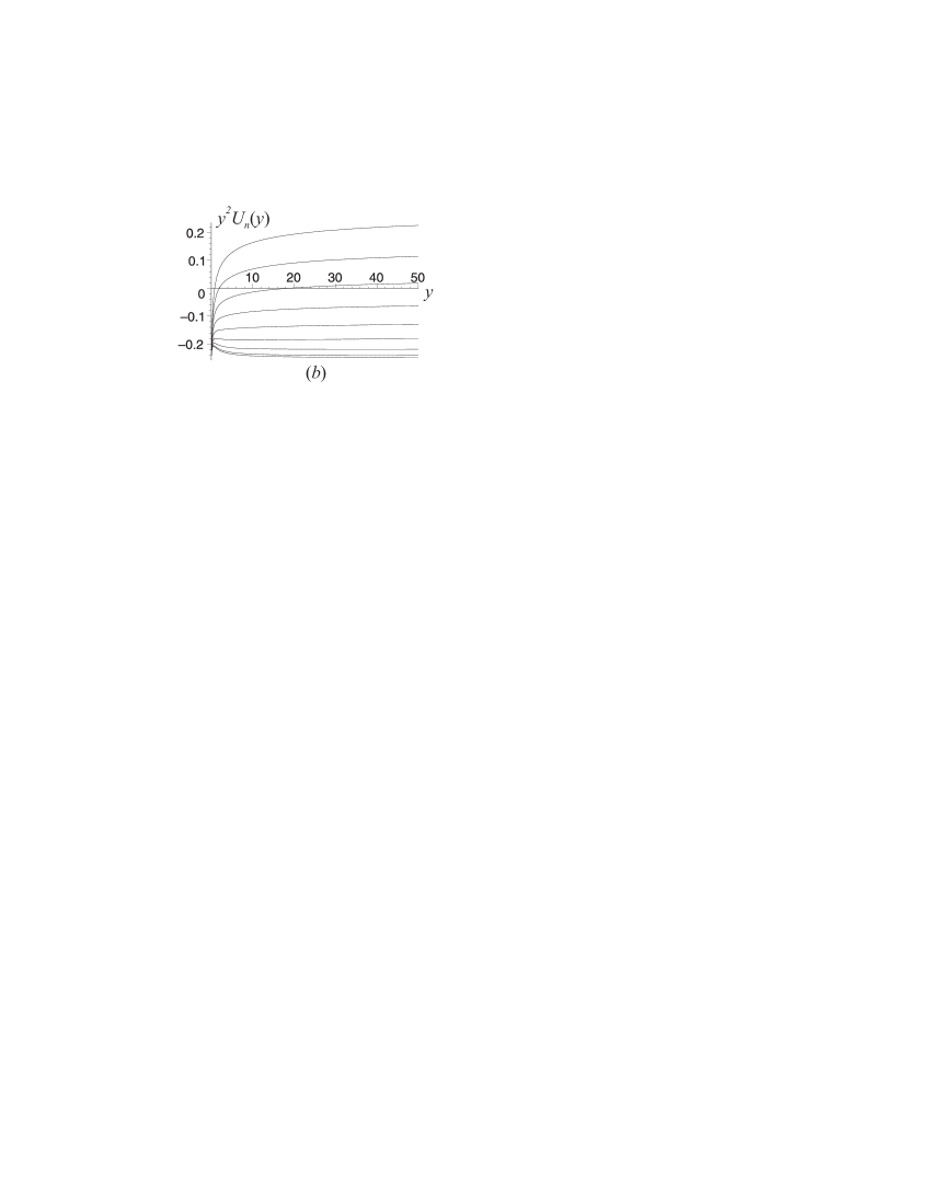
FIG. 1.: The graphs of the function $y^{2}U_{n=0}(y)$; (a) $\xi=0$; (b) $\xi=1/6$; the graphs corresponds to the values $m=0$, $0.1$, $0.2$, $0.3$, $0.4$, $0.5$, $0.6$, $0.7$, $0.8$ from bottom to top.

The graph of $y^{2}V(y)$ is given in the figure 2(a). Note that the function $V(y)$ is completely determined by ${\em h}(y)$ and does not depend on the parameters $m$ and $\xi$. In the figure 2(b) the ratio $\xi V/U_{n}$ is shown for $n=0$, $1$, $2$, $m=0.1$, and $\xi=1/6$.

 

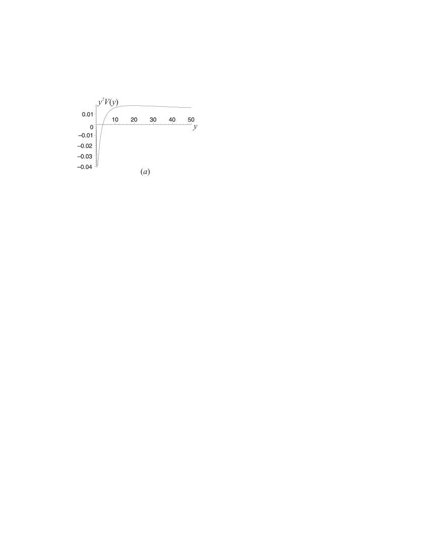
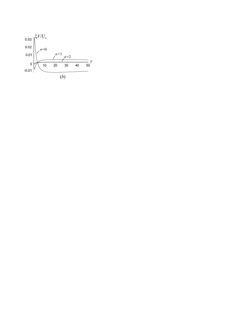
FIG. 2.: (a) The graph of the function $y^{2}V(y)$. (b) The ratio ${\xi V/U_{n}}$; $n=0,1,2$, $m=0.1$, $\xi=1/6$; $T=(4\pi)^{-1}$.

One has $|\xi V/U_{n}|\ll 1$. For example, $\max(|\xi V/U_{n}|)\approx 0.032$, $0.009$, $0.0002$ for $n=0$, $1$, $2$ respectively, so that the higher the number of mode the less the ratio $|\xi V/U_{n}|$.

Thus we may conclude that at least for 2D Schwarzschild metric the term $\xi V(y)$ is much less than $U_{n}(y)$ in the whole range of $y$. Using the smallness of $\xi V$ in comparison with $U_{n}$ we can neglect this term in the equation (47).

B The uniform approximation for the massless field modes

Consider the massless case, $m=0$, with arbitrary coupling $\xi$. Neglecting the term $\xi V$ in the equation (47) we obtain

$$\frac{d^{2}u}{dy^{2}}-\left(\frac{\omega_{n}^{2}-\frac{1}{4}}{y^{2}}+\frac{c\xi}{y(c+y)^{2}}\right)u=0,$$ (57)

or, after rescaling $y=c\tilde{y}$,

$$\frac{d^{2}u}{d\tilde{y}^{2}}-\left(\frac{\omega_{n}^{2}-\frac{1}{4}}{\tilde{y}^{2}}+\frac{\xi}{\tilde{y}(1+\tilde{y})^{2}}\right)u=0~{}.$$ (58)

Comparing with Eqs. (28), (30) we find two independent solutions of the equation (57):

$$u^{(1)}_{n} = y^{1/2+\omega_{n}}(c+y)^{-2\omega_{n}}F(a,b;2\omega_{n}+1;\frac{y}{c+y}),$$ (59)

$$u^{(2)}_{n} = y^{1/2+\omega_{n}}(c+y)^{-2\omega_{n}}F(a,b;2\omega_{n}+1;\frac{c}{c+y}),$$ (60)

with

$$a=\frac{1}{2}+2\omega_{n}+\frac{1}{2}\sqrt{1-4\xi},\quad b=\frac{1}{2}+2\omega_{n}-\frac{1}{2}\sqrt{1-4\xi}.$$

These functions represent an approximate solution of the equation (47) in case $m=0$.

C The uniform approximation for the massive field modes

Consider the massive case. Neglecting the term $\xi V$ in the equation (47) gives

$$\frac{d^{2}u}{dy^{2}}-\left(\frac{\omega_{n}^{2}-\frac{1}{4}}{y^{2}}+\frac{m^{2}{\em h}(y)}{y(c+y)}+\frac{c\xi}{y(c+y)^{2}}\right)u=0.$$ (61)

Generally this equation cannot be solved exactly, and so let us construct an approximate solution. For this aim we study asymptotical properties of the equation (61). First consider the region far from the horizon, $y\to\infty$. Neglecting terms of order $y^{-3}$ and smaller in the equation (61) we get

$$\left[\frac{d^{2}}{dy^{2}}-\frac{\omega_{n}^{2}-\frac{1}{4}+m^{2}{\em h}}{y^{2}}\right]u=0.$$ (62)

Introducing in the equation (62) a new variable by $dx_{*}=dy/y$ and using the relation $s(x_{*})=y^{-1/2}u(y)$ we obtain

$$\frac{d^{2}s}{dx_{*}^{2}}-\Omega_{n}^{2}(x_{*})s=0,$$ (63)

where

$$\Omega_{n}(x_{*})=\sqrt{\omega_{n}^{2}+m^{2}{\em h}}.$$ (64)

An approximate solution of the equation (63) can be written in the well-known WKB form:

$$s_{n}^{(1)}=\frac{1}{\sqrt{2\Omega_{n}}}\,\exp\left[\int\Omega_{n}dx_{*}\right],\quad s_{n}^{(2)}=\frac{1}{\sqrt{2\Omega_{n}}}\,\exp\left[-\int\Omega_{n}dx_{*}\right].$$ (65)

Returning to the variables $y$ and $u_{n}$ we obtain the WKB solution of the equation (62):

$$u_{n}^{(1)}=\frac{y^{1/2}}{\sqrt{2\Omega_{n}}}\,\exp\left[\int\Omega_{n}\frac{dy}{y}\right],\quad u_{n}^{(2)}=\frac{y^{1/2}}{\sqrt{2\Omega_{n}}}\,\exp\left[-\int\Omega_{n}\frac{dy}{y}\right].$$ (66)

These functions give an approximate solution of the equation (61) in the region $y\to\infty$.

Now consider the region near the horizon, $y\to 0$. Taking into account Eq.(50) and neglecting in the equation (61) terms of order $y^{-1}$ and smaller we get

$$\left[\frac{d^{2}}{dy^{2}}-\frac{\omega_{n}^{2}-\frac{1}{4}}{y^{2}}\right]u=0.$$ (67)

It is worth noting that the last equation does not contain the parameters $m$ and $\xi$. This means that any scalar field with arbitrary mass $m$ and coupling $\xi$ near a horizon behaves effectively like the conformal scalar field with $m=0$ and $\xi=0$. Two independent solutions of the equation (67) are

$$u_{n=0}^{(1)} = y^{1/2},\quad u_{n=0}^{(2)}=-y^{1/2}\ln y$$ (68)

$$u_{n>0}^{(1)} = \frac{1}{\sqrt{2\omega_{n}}}\,y^{\omega_{n}+1/2},\quad u_{n>0}^{(2)}=\frac{1}{\sqrt{2\omega_{n}}}\,y^{-\omega_{n}+1/2}.$$ (69)

Respectively, for the radial modes $s_{n}^{(1,2)}=y^{-1/2}u_{n}^{(1,2)}$ expressed in the coordinate $y$ [see Eq. (19)] we obtain

$$s_{n=0}^{(1)} = 1,\quad s_{n=0}^{(2)}=-\ln y$$ (70)

$$s_{n>0}^{(1)} = \frac{1}{\sqrt{2\omega_{n}}}\,y^{\omega_{n}},\quad s_{n>0}^{(2)}=\frac{1}{\sqrt{2\omega_{n}}}\,y^{-\omega_{n}}.$$ (71)

Note that the modes $s_{n}^{(1,2)}$ are normalized by the condition (14) which for the coordinate $y$ reads

$$s^{(1)}_{n}{ds^{(2)}_{n}\over dy}-s^{(2)}_{n}{ds^{(1)}_{n}\over dy}=-\frac{1}{y}.$$ (72)

Thus, we may summarize that a solution of the equation (61) should possess the asymptotical properties (66) and (70). We also assumed that terms containing derivatives of ${\em h}$ are small and can be neglected. At last, it should be taken into account that in case ${\em h}\equiv{\rm const}$ the equation (61) could be solved analytically with the solutions given by (30). Now combining these results we choose approximate solutions of the equation (61) as follows:

$$u_{n}^{(1)} = \frac{y^{1/2}}{\sqrt{2\Omega_{n}}}\,\exp\left[\int\Omega_{n}\frac{dy}{y}\right]\Psi_{n}^{(1)},$$ (73)

$$u_{n}^{(2)} = \frac{y^{1/2}}{\sqrt{2\Omega_{n}}}\,\exp\left[-\int\Omega_{n}\frac{dy}{y}\right]\Psi_{n}^{(2)},$$ (74)

with

$$\Psi_{n}^{(1)} = \frac{2\Omega_{n}}{W_{n}}\left(\frac{y}{c+y}\right)^{\omega_{n}+\Omega_{n}}y^{-2\Omega_{n}}F(a,b;2\omega_{n}+1;\frac{y}{c+y}),$$ (75)

$$\Psi_{n}^{(2)} = \left(\frac{y}{c+y}\right)^{\omega_{n}+\Omega_{n}}F(a,b;2\Omega_{n}+1;\frac{c}{c+y}).$$ (76)

It can be shown that the given functions $u_{n}^{(1,2)}$ possess all necessary properties. First, substituting the solutions (73) into the equation (61) one may see that they obey the equation up to terms containing derivatives of ${\em h}$. Second, using properties of the hypergeometric functions (see Ref. [15]) one can verify that the solutions (73) have the asymptotical form (70) and (66) at $y\to 0$ and $y\to\infty$, respectively. Moreover, note that the functions (73) reproduce the exact solution (30) in case ${\em h}\equiv{\rm const}$ or/and $m=0$.

Finally, using the relation $s(x)=y^{-1/2}u(y)$ and the formulas (73) gives an approximation for the radial modes $s^{(1,2)}_{n}.$ It is worth noting that this approximation has been derived for arbitrary mass $m$ of the scalar field (including $m=0$) and arbitrary coupling $\xi$. It is also important that the approximation works correctly both far from and near the horizon. For this reason we will call it as a uniform  approximation.

VI Evaluating of ${\langle\varphi^{2}\rangle}$ in the uniform approximation

Using the uniform approximation, we may obtain the radial Green functions ${\cal G}_{n}=s^{(1)}_{n}s^{(2)}_{n}$ and construct the approximate expression for ${\langle\varphi^{2}\rangle}_{\rm unren}$:

$${\langle\varphi^{2}\rangle}_{\rm unren}=T{\cal G}_{0}^{\rm ua}(x,x)+2T\sum_{n=1}^{\infty}\,\cos(2\pi nT\epsilon)\,{\cal G}_{n}^{\rm ua}(x,x),$$ (77)

where the superscript ‘ua’ is used to denote the uniform approximation.

We may simplify the resulting approximate expression for ${\langle\varphi^{2}\rangle}_{\rm unren}$ if we take into account that the $n>0$ modes are satisfactory described by the WKB approximation. In this case we will use the uniform approximation in order to compute ${\cal G}_{n=0}$ only, and use the WKB approximation in order to compute the other radial Green functions ${\cal G}_{n>0}$, so that

$${\langle\varphi^{2}\rangle}_{\rm unren}=T{\cal G}_{0}^{\rm ua}(x,x)+2T\sum_{n=1}^{\infty}\,\cos(2\pi nT\epsilon)\,{\cal G}_{n}^{\rm WKB}(x,x).$$ (78)

The corresponding calculations for $\langle T^{\mu}_{\nu}\rangle$ would require to use the uniform approximation for $n=1$ as well. Subtracting ${\langle\varphi^{2}\rangle}_{\rm DS}$ from ${\langle\varphi^{2}\rangle}_{\rm unren}$ and taking the limit $\epsilon\to 0$ gives the renormalized expression for ${\langle\varphi^{2}\rangle}$:

$${\langle\varphi^{2}\rangle}_{\rm ren}={\langle\varphi^{2}\rangle}_{0}+{\langle\varphi^{2}\rangle}_{1},$$ (79)

where we denote

$${\langle\varphi^{2}\rangle}_{0}=T{\cal G}_{0}^{\rm ua}(x,x),$$ (80)

and

$${\langle\varphi^{2}\rangle}_{1}=\lim_{\epsilon\to 0}\left[2T\sum_{n=1}^{\infty}\,\cos(2\pi nT\epsilon)\,{\cal G}_{n}^{\rm WKB}(x,x)-{\langle\varphi^{2}\rangle}_{\rm DS}\right].$$ (81)

Using the uniform approximation (73) for the radial modes $s=y^{-1/2}u$ and taking into account that

$$\omega_{0}=0,\quad\Omega_{0}=m\sqrt{{\em h}},\quad W_{0}=\frac{\Gamma(2m\sqrt{{\em h}}+1)}{\Gamma(a)\Gamma(b)},$$

$$a=\frac{1}{2}+m\sqrt{{\em h}}+\frac{1}{2}\sqrt{1-4\xi},\quad b=\frac{1}{2}+m\sqrt{{\em h}}-\frac{1}{2}\sqrt{1-4\xi},$$

we can write ${\langle\varphi^{2}\rangle}_{0}=T{\cal G}_{0}^{\rm ua}=Ts^{(1)}_{0}s^{(2)}_{0}$ as follows:

$${\langle\varphi^{2}\rangle}_{0} = \frac{T}{2\Omega_{0}}\Psi^{(1)}_{0}\Psi^{(2)}_{0}$$ (82)

$$= \frac{T\,\Gamma(a)\Gamma(b)}{\Gamma(2m\sqrt{{\em h}(y)}+1)}\left(\frac{1}{c+y}\right)^{2m\sqrt{{\em h}(y)}}F\left(a,b;1;\frac{y}{c+y}\right)F\left(a,b;2m\sqrt{{\em h}(y)}+1;\frac{c}{c+y}\right).$$ (83)

For a given spacetime the function ${\em h}$ and the parameter $c$ are known. Hence the expression (82) represents an analytical formula describing an approximation for ${\langle\varphi^{2}\rangle}_{0}$.

To evaluate ${\langle\varphi^{2}\rangle}_{1}$ one may use the well-elaborated summation procedure dealing with the WKB approximation (see, e.g., [3, 4], and also [14]). Combining Eqs.(34,40,81,A4), we obtain

$${\langle\varphi^{2}\rangle}_{1} = \frac{1}{4\pi}\left[\ln\left(\frac{\mu^{2}f}{2(2\pi T)^{2}}\right)+2C\right]+{1\over 2\pi}\,S_{0}$$ (85)

$$+T\left[-\frac{1}{2}\xi RfS_{1}-\frac{1}{8}m^{2}(f^{2}f^{\prime\prime}+f{f^{\prime}}^{2})S_{2}+\frac{5}{32}m^{4}f^{2}{f^{\prime}}^{2}S_{3}\right]$$

where

$$S_{0}=\sum_{n=1}^{\infty}\left[{1\over\sqrt{n^{2}+{m^{2}f\over(2\pi T)^{2}}}}-{1\over n}\right],$$ (86)

and

$$S_{k}=\sum_{n=1}^{\infty}\frac{1}{\left[(2\pi Tn)^{2}+m^{2}f\right]^{k+1/2}},\quad k=1,2,3,\dots.$$ (87)

All the sums $S_{j}$ in this formula converge everywhere and $S_{0}$ tends to zero at the horizon ($f\rightarrow 0$). The logarithmic term combined with ${\langle\varphi^{2}\rangle}_{0}$, which also logarithmically diverges at the horizon, leads to $(T-1/4\pi)\ln(f)$ term (see Appendix). In the Hartle-Hawking state $T=1/4\pi$ and, hence, total ${\langle\varphi^{2}\rangle}_{\rm ren}$ is finite, as it should be.

Thus the uniform approximation solves the problem of finiteness of $\langle\varphi^{2}\rangle$ at the horizon by accurately taking into account of the zero mode contribution. Nevertheless finiteness itself on the horizon does not guarantee the correct value. So, we should compare our approximation with numerical calculations to get an idea how precise it is. The most important contribution comes from zero modes, this is why we present here plots for comparison of only their contribution. For higher modes the WKB approximation works very well (see, e.g., [4, 14]

 

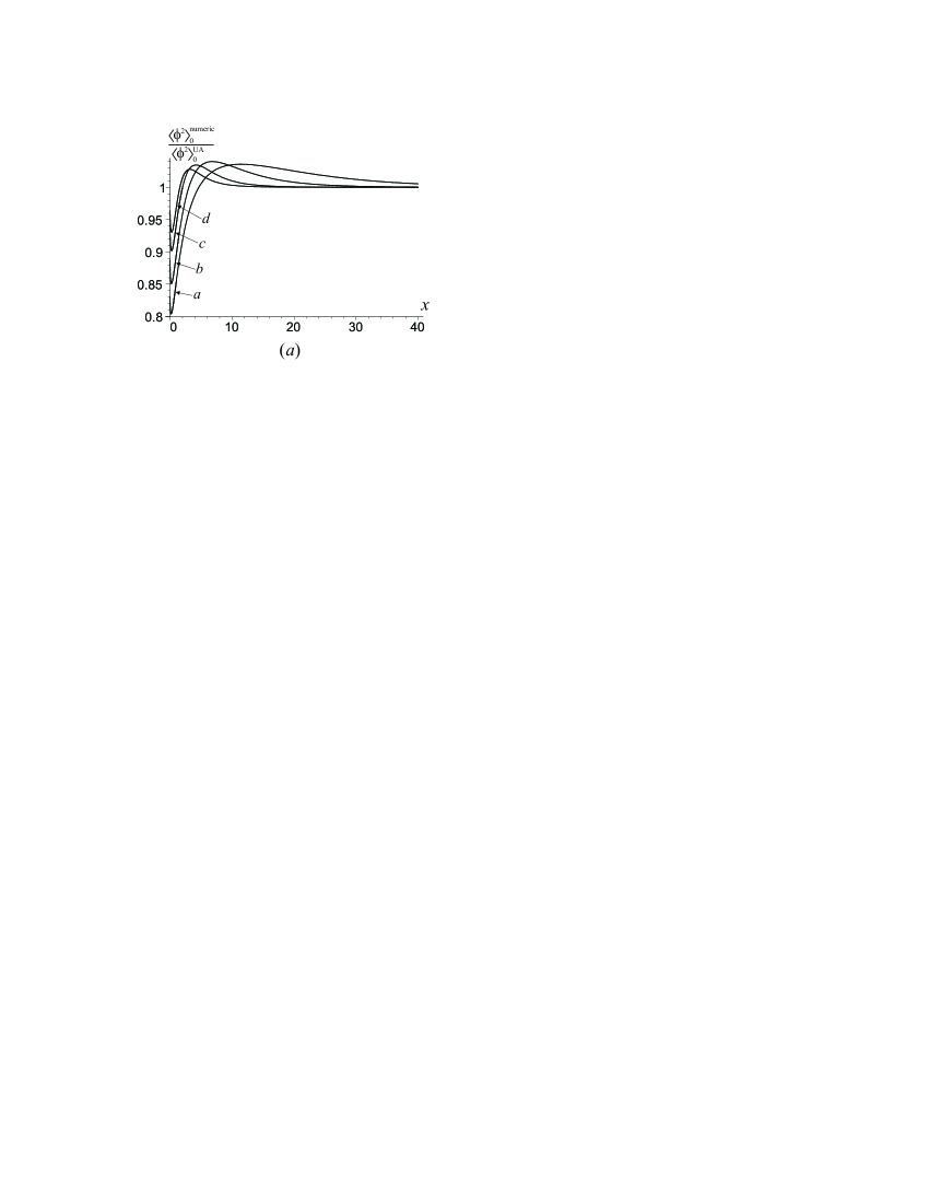
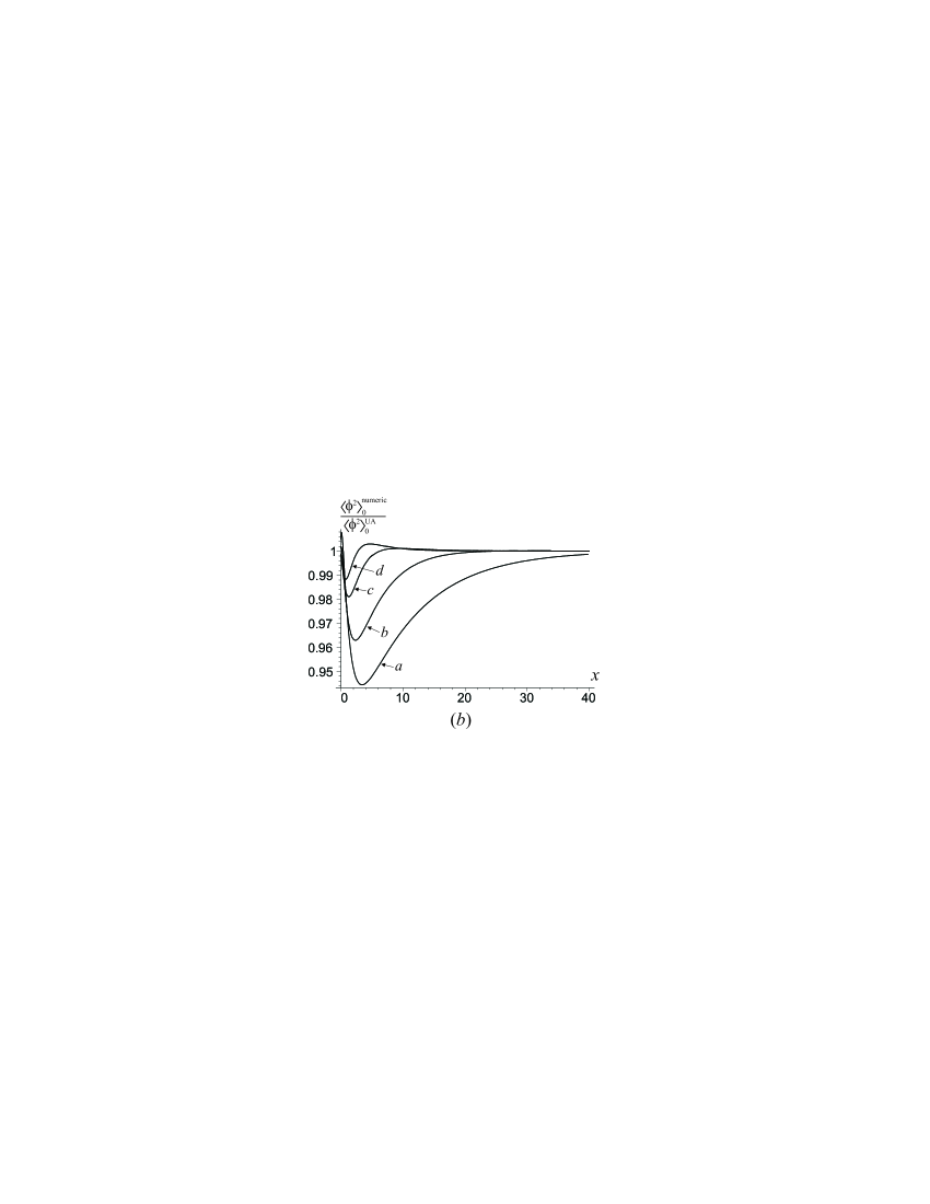
FIG. 3.: The graphs demonstrate the ratio of exact numerical calculations and the uniform approximation for ${\langle\varphi^{2}\rangle}_{0}$. The figures (a) and (b) correspond to $\xi=0$ and $\xi=1/6$, and the curves $a,b,c,d$ correspond to $m=0.05,0.1,0.2,0.3$, respectively.

One can see that the larger mass the more accurate becomes the uniform approximation. For $m\geq 1$ and $\xi\geq 1/6$ the uniform approximation gives practically exact value on the horizon and at infinity and the maximum deviation from exact function is less than 0.25%. For other parameters it is still very precise. This you can see in Fig.(3).

Let us summarize the obtained results. We demonstrated that the WKB approximation traditionally used for obtaining different analytical approximations for local observables breaks down for low frequency modes. In the general case this results in the logarithmic divergences of these observables at the black hole horizon. The adopted approximations can be improved if one uses a more accurate expression for the low frequency modes. We propose a method, which we call a uniform approximation, which not only automatically gives a finite value for local observables, but also provides a good approximation of the observables uniformly in the interval from the horizon to infinity. Our concrete calculations were done for $\langle\varphi^{2}\rangle$ in 2D black hole spacetime, but the proposed method can be used for other local observables and for higher dimensional black holes.

A Remarks on the $\log$-divergence of ${\langle\varphi^{2}\rangle}$ and $\langle T_{\mu\nu}\rangle$ near the horizon

In this appendix we discuss the problem which accompanies many of approximate methods [see, for example [6, 4, 9]] derived for calculating expectation values, such as ${\langle\varphi^{2}\rangle}$ and $\langle T_{\mu\nu}\rangle$, on the black hole background. The essence of the problem is that the approximate expressions for these values turn out to be proportional to $\ln f$ and hence diverge logarithmically near the horizon where $f\to 0$. It is important to stress that such the log-divergence takes place for both vacuum and thermal expectation values with any temperature, including the Hartle-Hawking state with the Hawking temperature. We will call this problem as the problem of  $\log$-divergence.

As we will see the problem of $\log$-divergence is tightly connected with accurate consideration and taking into account a contribution of zero modes into expectation values near the horizon. Really, as has been shown above the radial modes of a scalar field with arbitrary mass and coupling near the horizon have the asymptotical form (50). Then, the radial Green functions ${\cal G}_{n}=s_{n}^{(1)}s_{n}^{(2)}$ near the horizon are

$${\cal G}_{n=0}=-\ln y,$$ (A1)

$${\cal G}_{n>0}=\frac{1}{2\omega_{n}}=\frac{1}{4\pi nT},$$ (A2)

and the unrenormalized expression for ${\langle\varphi^{2}\rangle}$ reads

$$\langle\varphi^{2}\rangle_{\rm unren}=-T\ln y+\frac{1}{2\pi}\sum_{n=1}^{\infty}\frac{\cos(2\pi nT\epsilon)}{n},$$ (A3)

where $\epsilon=\tau-\tau^{\prime}$. Using the formula

$$\sum_{n=1}^{\infty}\frac{\cos(n\kappa\epsilon)}{n}=\frac{1}{2}\ln\left[\frac{1}{2\left(1-\cos(\kappa\epsilon)\right)}\right]=-\frac{1}{2}\ln\kappa^{2}\epsilon^{2}+{\cal O}(\epsilon^{2}),$$ (A4)

we obtain the asymptotical form for $\langle\varphi^{2}\rangle_{\rm unren}$ near the horizon:

$$\langle\varphi^{2}\rangle_{\rm unren}=-T\ln y-\frac{1}{4\pi}\ln\kappa^{2}\epsilon^{2}+{\cal O}(\epsilon^{2}),$$ (A5)

where $\kappa=2\pi T$. To calculate a renormalized expression for ${\langle\varphi^{2}\rangle}$ one should subtract from $\langle\varphi^{2}\rangle_{\rm unren}$ the DeWitt-Schwinger counerterms (17) and go to the limit $\epsilon\to 0$: ${\langle\varphi^{2}\rangle}_{\rm ren}=\lim_{\epsilon\to 0}\left({\langle\varphi^{2}\rangle}_{\rm unren}-{\langle\varphi^{2}\rangle}_{\rm DS}\right)$. Note that ${\langle\varphi^{2}\rangle}_{\rm DS}\sim-(4\pi)^{-1}\ln\sigma$, and $\sigma\sim f\epsilon^{2}$ in the limit $\epsilon\to 0$. Hence

$${\langle\varphi^{2}\rangle}_{\rm ren}\sim-T\ln y+(4\pi)^{-1}\ln f+{\cal O}(y^{0}).$$

Taking into account that $f\approx y$ at $y\to 0$ we rediscover the known result that ${\langle\varphi^{2}\rangle}_{\rm ren}$ is regular near the horizon provided the temperature has the Hawking value, $T=(4\pi)^{-1}$, otherwise ${\langle\varphi^{2}\rangle}_{\rm ren}$ diverges as $\ln y$.

It is worth noting that the term $(4\pi)^{-1}\ln f$ coming from the DeWitt-Schwinger counterterms ${\langle\varphi^{2}\rangle}_{\rm DS}$ is compensated by the term $T\ln y$ coming from the expression for the $n=0$ radial Green function ${\cal G}_{0}$. Thus we see that the zero modes play an important role in the problem of $\log$-divergence.

To illustrate this statement we consider the approximation derived by Anderson, Hiscock and Samuel [4]. They obtained the approximate expressions for ${\langle\varphi^{2}\rangle}$ and $\langle T_{\mu\nu}\rangle$ [see Eqs. (4.2), (4.3), (4.4)] which are proportional to $\ln f$ and hence diverge logarithmically near the horizon where $f\to 0$. The cause of this divergence can be easily explained now. Examining the procedure derived by Anderson, Hiscock and Samuel for computing ${\langle\varphi^{2}\rangle}$ and $\langle T_{\mu\nu}\rangle$ for the nonzero temperature case one faces with a necessity to calculate the mode sums over $n$. Since the authors use for this aim an expansion in inverse powers of $n$, they encounter the problem of including into the calculation scheme a contribution of the $n=0$ modes. To resolve this problem the authors impose a lower limit cutoff in the mode sums, which for the nonzero temperature case means merely discarding the $n=0$ contribution from the summation procedure (see a discussion in the section IV and the appendix E). But as was shown above, taking into account the $n=0$ modes is necessary for a compensation of the $\log$-contribution coming from the counterterms ${\langle\varphi^{2}\rangle}_{\rm DS}$ and $\langle T_{\mu\nu}\rangle_{\rm DS}$; otherwise, one gets the problem of log-divergence.

REFERENCES

- [1] K. W. Howard and P. Candelas, Phys. Rev. Lett.53, 403 (1984).
- [2] K. W. Howard, Phys. Rev. D30, 2532 (1984).
- [3] P.R. Anderson, Phys. Rev. D39 3785 (1989); P.R. Anderson, Phys. Rev. D41 1152 (1990).
- [4] P.R. Anderson, W.A. Hiscock, D. A. Samuel, Phys. Rev. D51 4337 (1995).
- [5] P. Candelas, Phys. Rev. D21, 2185 (1980).
- [6] D. N. Page, Phys. Rev. D 25, 1499 (1982);
- [7] M. R. Brown, A. C. Ottewill, Phys. Rev. D31 2514 (1985).
- [8] M. R. Brown, A. C. Ottewill and D. N. Page, Phys. Rev. D33 2840 (1986)
- [9] V.P. Frolov, A.I. Zelnikov, Phys. Rev. D35 3031 (1987).
- [10] V. Frolov, P. Sutton, A. Zelnikov, Phys. Rev. D61 024021 (2000).
- [11] H. Koyama, Y. Nambu, A. Tomimatsu, Mod.Phys.Lett. A15 815 (2000).
- [12] R. Balbinot, A. Fabbri, V. Frolov, P. Nicolini, P. Sutton, A. Zelnikov, Phys. Rev. D63 084029 (2001).
- [13] V. Frolov and A. Zelnikov, Phys. Rev. D 63, 125026 (2001);
- [14] S. V. Sushkov, Phys. Rev. D 62, 064007 (2000);
- [15] M. Abramowitz and I. A. Stegun, Handbook of Mathematical Functions, (US National Bureau of Standards, Washington, 1964).