KEK-TH-828

KIAS P02074

TUM-HEP-429/02

UT-ICEPP 02-07

Rotating black holes at future colliders:
Greybody factors for brane fields

Daisuke Ida
Department of Physics, Tokyo Institute of Technology,
Tokyo 152-8551, Japan

Kin-ya Oda
Physik Dept. T30e, TU München,
James Franck Str., D-85748 Garching, Germany

Seong Chan Park
Korea Institute for Advanced Study (KIAS),
Seoul 130-012, Korea

d.ida@th.phys.titech.ac.jp
odakin@ph.tum.de
spark@kias.re.kr

Abstract

We study theoretical aspects of the rotating black hole production and evaporation in the extra dimension scenarios with TeV scale gravity, within the mass range in which the higher dimensional Kerr solution provides good description. We evaluate the production cross section of black holes taking their angular momenta into account. We find that it becomes larger than the Schwarzschild radius squared, which is conventionally utilized in literature, and our result nicely agrees with the recent numerical study by Yoshino and Nambu within a few % error for higher dimensional case. In the same approximation to obtain the above result, we find that the production cross section becomes larger for the black hole with larger angular momentum. Second, we derive the generalized Teukolsky equation for spin 0, 1/2 and 1 brane fields in the higher dimensional Kerr geometry and explicitly show that it is separable in any dimensions. For five-dimensional (Randall-Sundrum) black hole, we obtain analytic formulae for the greybody factors in low frequency expansion and we present the power spectra of the Hawking radiation as well as their angular dependence. Phenomenological implications of our result are briefly sketched.

1 Introduction

The fundamental gravitational scale can be lowered down to TeV scale to remedy the hierarchy between the Planck and Higgs mass scales in the large extra dimension (ADD) scenario [1] (see also ref. [2] for its stringy realization).  In warped compactification (Randall-Sundrum) scenario, both of them are scaling together along the location in the warped extra dimension, leading again to the TeV fundamental scale at our visible brane [4]. When nature realizes such a TeV scale gravity scenario, it is predicted that black hole production will dominate over the two body scattering well above the fundamental scale, with the geometrical cross section of the order of the Schwarzschild radius squared (of the black hole mass equal to the center of mass (CM) energy of the scattering) [5]. Following the observation that black holes will mainly decay into the standard model fields on the brane rather than into the bulk modes [6], collider signatures of black hole production and evaporation are studied comprehensively in ref. [7] and independently in ref. [8].  These two pioneering works are applied in a lot of papers of the black hole phenomenology of the ultra-high energy cosmic neutrino signature [10, 11] and of the collider signatures [12, 13, 14]. (In ref. [15], it is claimed that the black hole production cross section would be exponentially suppressed rather than being geometrical; this is later answered by the semi-classical argument [16] and by the correspondence principle applied to the production cross sections of black holes and strings [21]. )

The black hole phenomenology opens up the fascinating possibility of the experimental investigation of the quantum gravity in the following sense. As is emphasized in ref. [7], the black hole production hides all the shorter distance processes than the Planck length scale behind the event horizon and there emerges infrared-ultraviolet duality, i.e., the larger the CM energy becomes, the better the semi-classical treatment [24] of the resultant black hole is (since the Hawking temperature of it becomes lower). In string theory, where its non-perturbative definition is not yet established, this kind of situation (duality) often appears so that one picture is valid in one limit while the other is valid in the opposite limit (see e.g. ref. [25] for review and also refs. [26, 21]). The region of true interest is the intermediate one at which both pictures break down and non-perturbative formulation of the quantum gravity (or string theory) becomes relevant. Given the status of the theoretical development, experimental signature of quantum gravity at this intermediate region would be observed as the discrepancy from the semi-classical behavior in the black hole picture valid at high energy limit. Therefore in order to investigate the quantum gravity effect, it is essential to predict this semi-classical behavior as precisely as possible. This is the main motivation of our work.

After the production phase (the “balding” phase), the black holes are well described by the higher dimensional Kerr solution [27] if the mass of the produced black hole ($\simeq$ the CM energy of the collision) is large enough to neglect the brane tension at the horizon and also small enough to neglect the topology and the curvature of the extra dimension(s) [7]. Within the LHC energy region, the former condition is satisfied (or marginal) and the latter is perfect in the ADD scenario [7, 8] while the former is the same as in the ADD scenario and the latter is satisfied in the Randall-Sundrum scenario (when the horizon radius is smaller than the curvature length scale which is one or two order(s) of magnitude larger than the Planck length scale )  [7, 11]. Throughout this paper, we assume that both the two conditions are satisfied.

The black hole emits most of its quanta (and hence loses most of its mass and angular momentum) through the Hawking radiation [24] when the above “large-enough” (former) condition is satisfied and hence a few hot quanta emitted in the final “Planck” phase, which cannot be treated semiclassically, does not consist of the main part of the decay product [7]. (Remember that the smaller the black hole becomes, the hotter the Hawking radiation.) In most literature the “spin-down” phase of the black hole evolution [7], in which the black hole shed its angular momentum, is simply neglected and the Schwarzschild black hole is used from the start relying on the four-dimensional result [32] that the half life for spin down is a few % of the black hole lifetime. To improve this “Schwarzschild approximation”, it is important to estimate the production cross section of the black holes with finite angular momenta. In ref. [33], the production cross section of rotating black holes is estimated from the quantum mechanical matrix element between the initial two-plane-waves state and the ‘black hole state’. In this paper, we take more conservative approach based on the (classical) geometrical cross section,  in the spirit [16] that a classical description should be more or less valid for the black hole production in order to avoid the Voloshin’s exponential suppression mentioned above.

The Hawking radiation is determined for each mode by the greybody factor [24, 31], i.e. the absorption probability (by the black hole) of an incoming wave of the corresponding mode. Unfortunately, the greybody factors have been calculated only for brane- and bulk-scalar modes with the Schwarzschild black hole at present [43]. In current black hole phenomenology, the Hawking radiation is either not considered (typically in the cosmic neutrino signature) or considered with the greybody factor in the geometrical optics limit. To study the evaporation of the higher dimensional black hole and to progress the phenomenology further, it is prerequisite to obtain the greybody factors of the brane fields (which are the main decay modes of the black hole as is mentioned above).

In this paper, we obtain the brane field equations generalizing the Teukolsky’s method in four dimensions [38, 40, 41, 42]. We show that they are separable into radial and angular parts. For the five-dimensional Kerr black hole, we find the analytic formulae of the greybody factors within the low frequency expansion.

In section 2, we present the geometrical production cross section of rotating black holes with finite angular momenta in the approximation neglecting the balding phase. Our result of the largest impact parameter $b_{\mathrm{max}}$ for the black hole formation turns out to be in good agreement with the numerical result by Yoshino and Nambu [20]. Within the same approximation, we find that the (differential) cross section linearly increases with the angular momentum for a given black hole mass ($\simeq$ CM energy). We also estimate the production of the exploding black ring and find that it will possibly form when there are many extra dimensions. In section 3, we study the Hawking radiation from the rotating black hole. First we derive the brane field equations for the spin 0, 1/2, and 1 brane fields from the induced metric on the brane in the higher dimensional Kerr black hole back ground and show that these equations are separable into radial and angular parts for any number of extra dimensions. Next we find the analytic expression for the greybody factors for brane fields for the rotating five-dimensional (Randall-Sundrum) black hole within the low frequency expansions. We present the power spectra as well as their angular dependence applying these greybody factors. In section 4, we present a summary and briefly comment on the phenomenological implications of our results.

2 Production of rotating black holes

First we briefly review the properties of the rotating $(4+n)$- dimensional black hole [27]. Since we assume that the large enough condition (explained in the Introduction) is satisfied, the charges of the black hole can be neglected; they are at most a few coming from the initial two particles. In general, higher dimensional black hole may have $\lfloor(n+3)/2\rfloor$ angular momenta. When the black hole is produced in the collision of two particles on the brane, where the initial state has only single angular momentum (directed in the brane), it is sufficient to consider that the only single angular momentum is non-zero [7]. (This implicitly assumes that the balding phase can be neglected, namely that the “junk” emissions are negligible and do not change the $\lfloor(n+3)/2\rfloor$ angular momenta during this phase.) In the Boyer-Lindquist coordinate, the metric for the black hole with single angular momentum takes the following form [27]

$$g = \left(1-\frac{\mu r^{-n+1}}{\Sigma(r,\vartheta)}\right)dt^{2}-\sin^{2}\vartheta\left(r^{2}+a^{2}+a^{2}\sin^{2}\vartheta\frac{\mu r^{-n+1}}{\Sigma(r,\vartheta)}\right)d\varphi^{2}$$ (1)

$$\mbox{}+2a\sin^{2}\vartheta\frac{\mu r^{-n+1}}{\Sigma(r,\vartheta)}dtd\varphi-\frac{\Sigma(r,\vartheta)}{\Delta(r)}dr^{2}-\Sigma(r,\vartheta)d\vartheta^{2}$$

$$\mbox{}-r^{2}\cos^{2}\vartheta\,d\Omega^{n},$$

where

$$\Sigma(r,\vartheta) = r^{2}+a^{2}\cos^{2}\vartheta,$$

$$\Delta(r) = r^{2}+a^{2}-\mu r^{-n+1}.$$

We can see that the horizon occurs when $\Delta(r)=0$, i.e. when $r=r_{h}$ with

$$r_{h} = \left[\frac{\mu}{1+a_{*}^{2}}\right]^{1/(n+1)}=(1+a_{*}^{2})^{-1/(n+1)}r_{S},$$ (2)

where $a_{*}=a/r_{h}$ and the Schwarzschild radius $r_{S}=\mu^{1/(n+1)}$ are introduced for later convenience. Note that there is only single horizon when $n\geq 1$ (contrary to the four-dimensional Kerr black hole which has inner and outer horizons) and its radius is independent of the angular coordinates. We can obtain the total mass $M$ and angular momentum $J$ of the black hole from the metric (1)

$$M=\frac{(n+2)A_{n+2}}{16\pi G}\mu,\hskip 28.45274ptJ=\frac{2}{n+2}Ma,$$ (3)

where $A_{n+2}$$=$$2\,\pi^{(n+3)/2}/\Gamma(\frac{n+3}{2})$ is the area of unit sphere $S^{n+2}$ and $G$ is the $(4+n)$-dimensional Newton constant. Therefore we may consider $\mu$ and $a$ (or $r_{h}^{-1}$ and $a_{*}$) as the normalized mass and angular momentum parameters, respectively. We note that there are no upper bound on $a$ when $n\geq 2$ nor on $a_{*}$ when $n\geq 1$, contrary to the four-dimensional case where both $a$ and $a_{*}$ are bounded from above. In this paper, we concentrate on the brane field equations and hence only the induced metric on the brane is relevant, where the last term in eq. (1) vanishes and the angular variables $\vartheta$ and $\varphi$ are redefined to take the values $0\leq\vartheta\leq\pi$ and $0\leq\varphi<2\pi$. The explicit form is given in eq. (98).

2.1 Production cross section

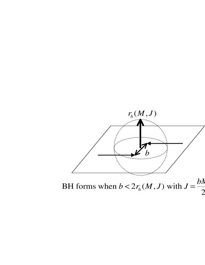
Figure 1: Schematic picture for the condition of the black hole formation.

We estimate the production cross section of rotating black holes within the classical picture. Let us consider a collision of two massless particles with finite impact parameter $b$ and CM energy $\sqrt{s}=M_{i}$ so that each particle has energy $M_{i}/2$ in the CM frame. The initial angular momentum before collision is $J_{i}=bM_{i}/2$ (in the CM frame). Suppose that a black hole forms whenever the initial two particles (characterized by $M_{i}$ and $J_{i}$) can be wrapped inside the event horizon of the black hole with the mass $M=M_{i}$ and angular momentum $J=J_{i}$ (see Fig. 1 for schematic picture), i.e., when

$$b < 2r_{h}(M,J)=2r_{h}(M_{i},bM_{i}/2),$$ (4)

where $r_{h}(M,J)$ is defined through eqs. (2) and (3). Since the right hand side is monotonically decreasing function of $b$, there is maximum value $b_{\mathrm{max}}$ which saturates the inequality (4)

$$b_{\mathrm{max}}(M)=2\left[1+\left(\frac{n+2}{2}\right)^{2}\right]^{-{1\over n+1}}r_{S}(M),$$ (5)

where $r_{S}(M)$ is defined by $r_{S}(M)=\mu(M)^{1/(n+1)}$ and eq. (3). When $b=b_{\mathrm{max}}$, the rotation parameter $a_{*}$ takes the maximal value $(a_{*})_{\mathrm{max}}=(n+2)/2$.

The formula (5) fits the numerical result of $b_{\mathrm{max}}$ with full consideration of the general relativity by Yoshino and Nambu [20] within the accuracy less than 1.5% for $n\geq 2$ and 6.5% for $n=1$ (although it just gives the Schwarzschild radius $b_{\mathrm{max}}=r_{S}(M)$ for $n=0$ which is 24% larger than the numerical result [18]):

$$\begin{array}[]{c|cccccccc}n&0&1&2&3&4&5&6&7\\ \hline\cr R_{\mathrm{Numerical}}~{}\cite[cite]{[\@@bibref{}{Yoshino:2002tx}{}{}]}&0.804&1.04&1.16&1.23&1.28&1.32&1.35&1.37\\ R_{\mathrm{Analytic}}&1.00&1.11&1.17&1.22&1.26&1.30&1.33&1.36\end{array},$$ (9)

where $R$ denotes $R=b_{\mathrm{max}}/r_{S}(M)$.

Our result is obtained in the approximation that we neglect all the effects by the junk emissions in the balding phase and hence that the initial CM energy $M_{i}$ and angular momentum $J_{i}$ become directly the resultant black hole mass $M=M_{i}$ and angular momentum $J=J_{i}$. The coincidence of our result with the numerical study [20] suggests that this approximation would be actually viable for higher dimensional black hole formation at least unless $b$ is very close to $b_{\mathrm{max}}$. 

Once we neglect the balding phase, hence the junk emission, the initial impact parameter $b$ directly leads to the resultant angular momentum of the black hole $J=bM/2$. Since the impact parameter $[b,b+db]$ contributes to the cross section $2\pi bdb$, this relation between $b$ and $J$ tells us the (differential) production cross section of the black hole with its mass $M$ and its angular momentum in $[J,J+dJ]$

$$d\sigma(M,J)=\left\{\begin{array}[]{cc}8\pi JdJ/M^{2}&(J<J_{\mathrm{max}})\\ 0&(J>J_{\mathrm{max}})\end{array}\right.,$$ (12)

where

$$J_{\mathrm{max}} = \frac{b_{\mathrm{max}}M}{2}=j_{n}\,\left(\frac{M}{M_{P}}\right)^{n+2\over n+1}$$ (13)

with

$$j_{n}=\left[2^{n}\pi^{n-3\over 2}\Gamma\left(n+3\over 2\right)\over(n+2)\left[1+\left(n+2\over 2\right)^{2}\right]\right]^{1/(n+1)},\hskip 28.45274ptM_{P}=\left((2\pi)^{n}\over 8\pi G\right)^{1/(n+2)}.$$ (14)

The numerical values for $j_{n}$ are summarized in Table 1.

Table 1: Numerical values for $j_{n}$ and $k_{n}$

$$\begin{array}[]{|c|cccccccc|}\hline\cr n&0&1&2&3&4&5&6&7\\ \hline\cr j_{n}&0.0398&0.256&0.531&0.815&1.09&1.37&1.63&1.88\\ k_{n}&0.0159&0.125&0.228&0.251&0.214&0.155&0.101&0.0603\\ k_{n}/j_{n}&0.399&0.489&0.429&0.308&0.195&0.114&0.0619&0.0320\\ \hline\cr\end{array}$$

It is observed that the differential cross section (12) linearly increases with the angular momentum. We expect that this behavior is correct as the first approximation, so that the black holes tend to be produced with larger angular momenta. At the typical LHC energy $M/M_{P}=5$, the value of $J_{\mathrm{max}}$ is $J_{\mathrm{max}}=2.9,4.5,\ldots,10,12$ for $n=1,2,\ldots,6,7$, respectively. This means that the semi-classical treatment of the angular momentum becomes increasingly valid for large $n$.

Integrating the expression (12) simply gives

$$\sigma(M) = \pi b_{\mathrm{max}}^{2}=4\left[1+\left(\frac{n+2}{2}\right)^{2}\right]^{-2/(n+1)}\,\pi r_{S}(M)^{2}$$ (16)

$$= F\,\pi r_{S}(M)^{2}.$$

The factor $F$ is summarized as

$$\begin{array}[]{c|cccccccc}n&0&1&2&3&4&5&6&7\\ \hline\cr F_{\mathrm{Numerical}}~{}\cite[cite]{[\@@bibref{}{Yoshino:2002tx}{}{}]}&0.647&1.084&1.341&1.515&1.642&1.741&1.819&1.883\\ F_{\mathrm{Analytic}}&1.000&1.231&1.368&1.486&1.592&1.690&1.780&1.863\end{array}.$$ (20)

This result implies that, apart from the four-dimensional case, we would underestimate the production cross section of black holes if we did not take the angular momentum into account and that it becomes more significant for higher dimensions. We point out that this effect has been often overlooked in the literature.

2.2 Rotating black ring

In four dimensions, the topology of the event horizon must be homeomorphic to two-sphere and there is a uniqueness theorems for static or stationary black holes. On the other hand, a higher-dimensional black hole can have various nontrivial topology [47], and the uniqueness property of stationary black holes fails in five (and probably in higher) dimensions. The typical example in five dimensions has been recently given by Emparan and Reall [48]. They have explicitly provided a solution of the five-dimensional vacuum Einstein equation, which represents the stationary rotating black ring (homeomorphic to $S^{1}\times S^{2}$). In this case, the centrifugal force prevents the black ring from collapsing. When the angular momentum is not large enough, the black ring will collapse to the Kerr black hole due to the gravitational attraction and some effective tension of the ring source. In fact, this five dimensional black ring solution has the minimum possible value of the angular momentum given by

$$J_{\mathrm{min}}=k_{\mathrm{BR}}\left(M\over M_{P}\right)^{3/2},$$ (21)

where $k_{\mathrm{BR}}=0.282$. On the other hand, we have the upper bound for the angular momentum of the black holes produced by particle collisions:

$$J_{\mathrm{max}}=j_{1}\left(M\over M_{P}\right)^{3/2},$$ (22)

where $j_{1}=0.256$. Since these numerical values are of the same order, we cannot conclude the possibility of black ring productions at colliders.

Here we consider the possibility of the higher dimensional black ring which is homeomorphic to $S^{1}\times S^{n}$. Corresponding Newtonian situation will be the system of a rotating massive circle. They are always unstable in higher dimensions; a circle with slow rotation collapses and one with rapid rotation explodes toward infinitely large thin circle. In general relativity, we have no idea as to the validity of this picture due to the nonlinearity of the Einstein equation. We shall discuss in the following the possibility of the black ring formation based on Newtonian picture assuming that the nonlinear effects of the gravity unchange the qualitative feature. For simplicity, we just consider the gravitational attraction and the centrifugal force of the massive circle and neglect the effect of tension. Let $\ell$, $M$ and $J$ be the radius, the mass and the angular momentum of the massive circle. Then we obtain ($3+n$)-dimensional effective theory with the Newton constant $G/2\pi\ell$ by integrating out along the $S^{1}$-direction. The Schwarzschild radius of the point mass in the effective theory is given by

$$r \sim \left[\frac{16\pi G}{(n+1)A_{n+1}}\frac{M}{2\pi l}\right]^{1/n}=\left[\frac{8GM}{(n+1)lA_{n+1}}\right]^{1/n}.$$ (23)

Thus we expect the black ring with $S^{1}$-radius $\ell$ and $S^{n}$-radius $r$. In flat space picture, $\ell>r$ should hold for black ring. This condition gives

$$\ell \mathrel{\mathchoice{\lower 3.0pt\vbox{\halign{$\m@th\displaystyle\hfill#\hfil$\cr>\crcr\sim\crcr}}}{\lower 3.0pt\vbox{\halign{$\m@th\textstyle\hfill#\hfil$\cr>\crcr\sim\crcr}}}{\lower 3.0pt\vbox{\halign{$\m@th\scriptstyle\hfill#\hfil$\cr>\crcr\sim\crcr}}}{\lower 3.0pt\vbox{\halign{$\m@th\scriptscriptstyle\hfill#\hfil$\cr>\crcr\sim\crcr}}}} \ell_{\mathrm{min}}=\left[8GM\over(n+1)A_{n+1}\right]^{1/(n+1)}.$$ (32)

On the other hand, the condition that the centrifugal force dominates against the gravitational attraction becomes

$$J \mathrel{\mathchoice{\lower 3.0pt\vbox{\halign{$\m@th\displaystyle\hfill#\hfil$\cr>\crcr\sim\crcr}}}{\lower 3.0pt\vbox{\halign{$\m@th\textstyle\hfill#\hfil$\cr>\crcr\sim\crcr}}}{\lower 3.0pt\vbox{\halign{$\m@th\scriptstyle\hfill#\hfil$\cr>\crcr\sim\crcr}}}{\lower 3.0pt\vbox{\halign{$\m@th\scriptscriptstyle\hfill#\hfil$\cr>\crcr\sim\crcr}}}} 2^{-(n+3)/2}G^{1/2}\ell^{-(n-1)/2}M^{3/2}.$$ (41)

This combined with eq. (32) gives the minimum value of the angular momentum for exploding black ring:

$$J \mathrel{\mathchoice{\lower 3.0pt\vbox{\halign{$\m@th\displaystyle\hfill#\hfil$\cr>\crcr\sim\crcr}}}{\lower 3.0pt\vbox{\halign{$\m@th\textstyle\hfill#\hfil$\cr>\crcr\sim\crcr}}}{\lower 3.0pt\vbox{\halign{$\m@th\scriptstyle\hfill#\hfil$\cr>\crcr\sim\crcr}}}{\lower 3.0pt\vbox{\halign{$\m@th\scriptscriptstyle\hfill#\hfil$\cr>\crcr\sim\crcr}}}} J_{\mathrm{min}}=k_{n}\left(M\over M_{P}\right)^{(n+2)/(n+1)},$$ (50)

where

$$k_{n} = 2^{-{2n^{2}+3n+7\over 2(n+1)}}\pi^{(n+6)(n-1)\over 4(n+1)}\left[\Gamma\left(n+2\over 2\right)\over n+1\right]^{-{n-1\over 2(n+1)}}.$$ (51)

The numerical values for $k_{n}$ are presented in Table 1. This result shows that $J_{\mathrm{min}}$ for exploding black rings is one or two order(s) of magnitude smaller than $J_{\mathrm{max}}$ for collision limit when $n$ is large. Therefore we expect that the exploding black rings are possibly produced at colliders if there are many extra dimensions, though they will suffer from the black string instability when they become sufficiently large thin rings. In the following of this paper, we do not follow the evolution of the exploding black ring nor consider the radiations from it since this is still at the heuristic stage; we concentrate on the Hawking radiations from the higher dimensional Kerr black hole after the balding phase.

3 Radiations from rotating black hole

In this section, we study the Hawking radiation [24] from the higher dimensional Kerr black hole [27]. The Hawking radiation is thermal but not strictly black body due to the frequency dependent greybody factor $\Gamma$, which is identical to the absorption probability (by the hole) of the corresponding mode [24, 31]. The quantity $1-\Gamma$ for each mode can be computed from the solution (to the wave equation of that mode) having no outgoing flux at the horizon as the ratio of the incoming and outgoing flux at infinity.

It can be shown that the higher dimensional black hole radiates comparable amount of energy into one brane mode and into one bulk mode (with all the Kaluza-Klein tower summed up) [6]. Typically, the number of degrees of freedom is much larger for brane mode than for bulk mode, i.e., tens of the standard-model degrees of freedom are living on the brane while there are only few degrees of freedom of the graviton (and possibly other fields) in the bulk. Therefore the higher dimensional black hole radiates mainly on the brane [6]. For this reason, we concentrate on the greybody factors for the brane mode in this paper.

3.1 Brane field equations

We derive the wave equations of the brane modes using the induced four dimensional metric of the $(4+n)$-dimensional rotating black hole [27]. The wave equations can be understood as generalization of the Teukolsky equation [38, 40, 41, 42] to the higher dimensional Kerr geometry. The derivation is shown in Appendix.

We present the brane field equations for massless spin $s$ field which are obtained from the metric (1) with the standard decomposition

$$\Phi_{s}=R_{s}(r)S(\vartheta)e^{-i\omega t+im\varphi},$$ (52)

utilizing the Newman-Penrose formalism [51]

$${1\over\sin\vartheta}{d\over d\vartheta}\left(\sin\vartheta{dS\over d\vartheta}\right)$$

$${}+\left[(s-a\omega\cos\vartheta)^{2}-(s\cot\vartheta+m\csc\vartheta)^{2}-s(s-1)+A\right]S=0,$$

(53)

$$\Delta^{-s}{d\over dr}\left(\Delta^{s+1}{dR\over dr}\right)+\Biggl{[}{K^{2}\over\Delta}+s\left(4i\omega r-i{[2r+(n-1)\mu r^{-n}]K\over\Delta}-n(n-1)\mu r^{-n-1}\right)$$

$${}+2ma\omega-a^{2}\omega^{2}-A\Biggl{]}R=0.$$ (54)

where

$$K = (r^{2}+a^{2})\omega-ma.$$ (55)

The solution of eq. (53) is called spin-weighted spheroidal harmonics ${}_{s}S_{lm}$ (see e.g. ref. [41, 52]) which reduces to the spin-weighted spherical harmonics ${}_{s}Y_{lm}$ (see e.g. ref. [53]) in the limit $a\omega\ll 1$,

$${}_{s}S_{lm}(a\omega;\vartheta,\varphi) = {}_{s}Y_{lm}(\vartheta,\varphi)+O(a\omega),$$ (56)

where

$${}_{s}Y_{lm}(\vartheta,\varphi) = (-1)^{m}e^{im\varphi}\left[\frac{(l+m)!(l-m)!}{(l+s)!(l-s)!}\frac{2l+1}{4\pi}\right]^{1/2}\left(\sin\frac{\vartheta}{2}\right)^{2l}$$ (61)

$$\mbox{}\times\sum_{j}\left(\begin{array}[]{c}l-s\\ j\\ \end{array}\right)\left(\begin{array}[]{c}l+s\\ j+s-m\\ \end{array}\right)(-1)^{l-j-s}\left(\cot\frac{\vartheta}{2}\right)^{2j+s-m},$$

with the sum over $j$ being understood in the range satisfying both $0\leq j\leq l-s$ and $0\leq j+s-m\leq l+s$. In this limit, the eigenvalue $A$ becomes $A=A_{0}+O(a\omega)$ where $A_{0}=l(l+1)-s(s+1)$ is defined for later convenience.

We may easily check that the radial equation (54) reduces to the Teukolsky equation [38, 40, 41, 42] when $n=0$ (hence $\mu=2GM$). The asymptotic solutions of eq. (54) at the horizon and infinity are obtained in the same way as in four dimensions [42]

$$\begin{array}[]{cc|cc}\lx@intercol\hfil r\rightarrow\infty\hfil\lx@intercol&\lx@intercol\hfil r\rightarrow r_{h}\hfil\lx@intercol\\ \mathrm{outgoing}&\mathrm{ingoing}&\mathrm{outgoing}&\mathrm{ingoing}\\ \hline\cr e^{i\omega r_{*}}/r^{2s+1}&e^{-i\omega r_{*}}/r&e^{ikr_{*}}&\Delta^{-s}e^{-ikr_{*}}\end{array}$$ (66)

where

$$k=\omega-\frac{ma}{r_{h}^{2}+a^{2}},$$ (67)

and $r_{*}$ is defined by $r_{*}\rightarrow r$ for $r\rightarrow\infty$ and

$$\frac{dr_{*}}{dr}=\frac{r^{2}+a^{2}}{\Delta(r)}.$$ (68)

3.2 Hawking radiation and greybody factor

Since we have shown that the massless brane field equations are separable into radial and angular parts, we may write down the power spectrum of the Hawking radiation [24] for each massless brane mode

$$\frac{dE_{s,l,m}}{dt\,d\omega\,d\varphi\,d\cos\vartheta} = \frac{1}{2\pi}\frac{{}_{s}\Gamma_{l,m}(r_{h},a;\omega)}{e^{(\omega-m\Omega)/T}-(-1)^{2s}}\left|{}_{s}S_{lm}(a\omega;\vartheta,\varphi)\right|^{2}\omega,$$ (69)

where $T$ and $\Omega$ are the Hawking temperature and the angular velocity at the horizon, respectively given by

$$T=\frac{(n+1)+(n-1)a_{*}^{2}}{4\pi(1+a_{*}^{2})r_{h}},\hskip 28.45274pt\Omega=\frac{a_{*}}{(1+a_{*}^{2})r_{h}},$$ (70)

and ${}_{s}\Gamma_{l,m}(r_{h},a;\omega)$ is the greybody factor [24, 31] which is identical to the absorption probability of the incoming wave of the corresponding mode. (In this paper we only consider the modes which can be treated as massless compared with the Hawking temperature $T$ since the emissions from massive modes are Boltzmann suppressed; Typically the standard model fields can be treated as massless at the LHC energy range.) Integrating eq. (69) by the angular variables, we obtain

$$\frac{dE_{s,l,m}}{dt\,d\omega} = \frac{1}{2\pi}\frac{{}_{s}\Gamma_{lm}}{e^{(\omega-m\Omega)/T}-(-1)^{2s}}\omega.$$ (71)

In the limit $a\omega\ll 1$ we can also write down the angular dependent power spectrum utilizing eq. (56)

$$\frac{dE}{dt\,d\cos\vartheta\,d\omega} = \frac{1}{2\pi}\frac{{}_{s}\Gamma_{lm}}{e^{(\omega-m\Omega)/T}-(-1)^{2s}}\omega\left[\int_{0}^{2\pi}d\varphi|{}_{s}Y_{lm}(\vartheta,\varphi)|^{2}\right],$$ (72)

where the integral in the square brackets can be done with eq. (LABEL:eq:spherical_harmonics); we summarize the results for the leading modes in the following table.

$$\begin{array}[]{|ccc|c|}\hline\cr s&l&m&\int_{0}^{2\pi}d\varphi|{}_{s}Y_{lm}(\vartheta,\varphi)|^{2}\\ \hline\cr 0&0&0&1/2\\ 0&1&1&(3/4)\sin^{2}\vartheta\\ 0&1&0&(3/2)\cos^{2}\vartheta\\ 0&1&-1&(3/4)\sin^{2}\vartheta\\ \hline\cr 1/2&1/2&1/2&\sin^{2}(\vartheta/2)\\ 1/2&1/2&-1/2&\cos^{2}(\vartheta/2)\\ \hline\cr 1&1&1&(3/8)(1-\cos\vartheta)^{2}\\ 1&1&0&(3/4)\sin^{2}\vartheta\\ 1&1&-1&(3/8)(1+\cos\vartheta)^{2}\\ \hline\cr\end{array}$$

Approximately, the time dependence of $M$ and $J$ can be determined by

$$-\frac{d}{dt}\left(\begin{array}[]{c}M\\ J\end{array}\right) = \frac{1}{2\pi}\sum_{s,l,m}g_{s}\int_{0}^{\infty}d\omega\frac{{}_{s}\Gamma_{l,m}(r_{h},a;\omega)}{e^{(\omega-m\Omega)/T}-(-1)^{2s}}\left(\begin{array}[]{c}\omega\\ m\end{array}\right),$$ (78)

where $g_{s}$ is the number of ‘massless’ degrees of freedom at temperature $T$, namely the number of degrees of freedom whose masses are smaller than $T$, with spin $s$. (Typically $g_{0}=4$, $g_{\frac{1}{2}}=90$ and $g_{1}=24$ when $T>m_{t},m_{H}$ and $g_{0}=0$, $g_{\frac{1}{2}}=78$ and $g_{1}=18$ when $m_{b}<T<m_{W}$ for the standard model fields.) Therefore, once we obtain the greybody factors, we completely determine the Hawking radiation and the subsequent evolution of the black hole up to the Planck phase, at which the semi-classical description by the Hawking radiation breaks down and a few quanta radiated is not predictable.

In the high frequency limit, the absorption cross section for each mode $\sigma=(\pi/\omega^{2})\Gamma$ is supposed to reach the geometrical optics limit (see e.g. refs. [13, 14])

$$\sigma_{g.o.}=\pi\left(\frac{n+3}{2}\right)^{2/(n+1)}\frac{n+3}{n+1}r_{H}^{2}.$$ (79)

In all the phenomenological literature this limit have been applied when one calculate the Hawking radiation. (In the refs. [13, 14] phenomenological weighting factors 2/3 and 1/4 are multiplied to eq.(79) for $s=1/2$ and $s=1$ fields, respectively, based on the result in four dimensions [31].)

3.3 Greybody factors for Randall-Sundrum black hole

To obtain the greybody factors from eqs. (53) and (54) in general dimensions, we need the numerical calculation, which is beyond the scope of this paper and will be shown in ref. [54]. In this paper we present analytic expression of the greybody factors of brane fields for $n=1$ Randall-Sundrum black hole within the low frequency expansion. Here we outline our procedure: First we obtain the “near horizon” and “far field” solutions in the corresponding limits; Then we match these two solutions at the “overwrapping region” in which both limits are consistently satisfied; Finally we impose the “purely ingoing” boundary condition at the near horizon side and then read the coefficients of “outgoing” and “ingoing” modes at the far field side; The ratio of these two coefficients can be translated into the absorption probability of the mode, which is nothing but the greybody factor itself.

First for convenience, we define dimensionless quantities

$$\xi=\frac{r-r_{h}}{r_{h}},\hskip 28.45274pt\widetilde{\omega}=r_{h}\omega,\hskip 28.45274pt\widetilde{Q}=\frac{\omega-m\Omega}{2\pi T}=(1+a_{*}^{2})\widetilde{\omega}-ma_{*}.$$ (80)

(Note that in the Schwarzschild limit $a_{*}\rightarrow 0$, $\widetilde{Q}$ becomes $\widetilde{Q}\rightarrow\widetilde{\omega}$.) Then the radial equation (54) becomes

$$\xi^{2}(\xi+2)^{2}R_{,\xi\xi}+2(s+1)\xi(\xi+1)(\xi+2)R_{,\xi}+\widetilde{V}R=0,$$ (81)

where

$$\widetilde{V} = \left[\widetilde{\omega}\xi(\xi+2)+\widetilde{Q}\right]^{2}+2is\widetilde{\omega}\xi(\xi+1)(\xi+2)-2is\widetilde{Q}(\xi+1)$$ (82)

$$\mbox{}-[A_{0}+O(a_{*}\widetilde{\omega})]\xi(\xi+2).$$

In the near horizon limit $\widetilde{\omega}\xi\ll 1$, the potential (82) becomes

$$\widetilde{V}=\widetilde{Q}^{2}-2is(\xi+1)\widetilde{Q}-A_{0}\xi(\xi+2)+O(\widetilde{\omega}\xi),$$ (83)

and the solution of eq. (81) with the potential (83) is obtained with the hypergeometric function

$$R_{\mathrm{NH}}=$$

$$C_{1}\left(\frac{\xi}{2}\right)^{-s-\frac{i\widetilde{Q}}{2}}\left(1+\frac{\xi}{2}\right)^{-s+\frac{i\widetilde{Q}}{2}}{}_{2}F_{1}(-l-s,l-s+1,1-s-i\widetilde{Q};-\frac{\xi}{2})$$

$$\mbox{}+C_{2}\left(\frac{\xi}{2}\right)^{\frac{i\widetilde{Q}}{2}}\left(1+\frac{\xi}{2}\right)^{-s+\frac{i\widetilde{Q}}{2}}{}_{2}F_{1}(-l+i\widetilde{Q},l+1+i\widetilde{Q},1+s+i\widetilde{Q};-\frac{\xi}{2}).$$

To impose the ingoing boundary condition at the horizon (66), i.e.

$$R\sim\xi^{-s}e^{-ikr_{*}},\hskip 28.45274ptk\frac{dr_{*}}{d\xi}\sim\frac{\widetilde{Q}}{2\xi},$$ (85)

we put $C_{2}=0$ and normalize $C_{1}=1$ without loss of generality and then we obtain

$$R_{\mathrm{NH}}=$$

$$\left(\frac{\xi}{2}\right)^{-s-\frac{i\widetilde{Q}}{2}}\left(1+\frac{\xi}{2}\right)^{-s+\frac{i\widetilde{Q}}{2}}{}_{2}F_{1}(-l-s,l-s+1,1-s-i\widetilde{Q};-\frac{\xi}{2}).$$

In the far field limit $\xi\gg 1+|\widetilde{Q}|$, the eq.(81) becomes

$$0=R_{,\xi\xi}+\frac{2(s+1)}{\xi}R_{,\xi}$$ (87)

$$+\left[\widetilde{\omega}^{2}+\frac{2i\widetilde{\omega}}{\xi}(s-2i\widetilde{\omega})-\frac{1}{\xi^{2}}\left[A_{0}+O(\widetilde{\omega})\right]+O(\xi^{-3})\right]R,$$

and the solution is obtained by the Kummer’s confluent hypergeometric function

$$R_{\mathrm{FF}} = B_{1}e^{-i\widetilde{\omega}\xi}\left(\frac{\xi}{2}\right)^{l-s}{}_{1}F_{1}(l-s+1,2l+2;2i\widetilde{\omega}\xi)$$ (88)

$$\mbox{}+B_{2}e^{-i\widetilde{\omega}\xi}\left(\frac{\xi}{2}\right)^{-l-s-1}{}_{1}F_{1}(-l-s,-2l;2i\widetilde{\omega}\xi),$$

where singularity from $2l$ being integer is regularized by the higher order terms in $\widetilde{\omega}$.

Matching the NH and FF solutions (LABEL:eq:NHsoltion) and (88) in the overlapping region $1+|\widetilde{Q}|\ll\xi\ll 1/\widetilde{\omega}$, we obtain

$$B_{1}=\frac{\Gamma(2l+1)\Gamma(1-s-i\widetilde{Q})}{\Gamma(l-s+1)\Gamma(l+1-i\widetilde{Q})},\hskip 14.22636ptB_{2}=\frac{\Gamma(-2l-1)\Gamma(1-s-i\widetilde{Q})}{\Gamma(-l-s)\Gamma(-l-i\widetilde{Q})}.$$ (89)

Then we extend the obtained FF solution toward the region $\xi\gg 1/\widetilde{\omega}$

$$R_{\infty}=Y_{\rm in}e^{-i\widetilde{\omega}\xi}\left(\frac{\xi}{2}\right)^{-1}+Y_{\rm out}e^{i\widetilde{\omega}\xi}\left(\frac{\xi}{2}\right)^{-2s-1},$$ (90)

where

$$Y_{\rm in} = \frac{\Gamma(2l+1)\Gamma(2l+2)}{\Gamma(l-s+1)\Gamma(l+s+1)}\frac{\Gamma(1-s-i\widetilde{Q})}{\Gamma(l+1-i\widetilde{Q})}(-4i\widetilde{\omega})^{-l+s-1}$$

$$\mbox{}+\frac{\Gamma(-2l)\Gamma(-2l-1)}{\Gamma(-l-s)\Gamma(-l+s)}\frac{\Gamma(1-s-i\widetilde{Q})}{\Gamma(-l-i\widetilde{Q})}(-4i\widetilde{\omega})^{l+s},$$

$$Y_{\rm out} = \frac{\Gamma(2l+1)\Gamma(2l+2)}{[\Gamma(l-s+1)]^{2}}\frac{\Gamma(1-s-i\widetilde{Q})}{\Gamma(l+1-i\widetilde{Q})}(4i\widetilde{\omega})^{-l-s-1}$$ (91)

$$\mbox{}+\frac{\Gamma(-2l)\Gamma(-2l-1)}{[\Gamma(-l-s)]^{2}}\frac{\Gamma(1-s-i\widetilde{Q})}{\Gamma(-l-i\widetilde{Q})}(4i\widetilde{\omega})^{l-s}.$$

Let us define $R_{-s}$ as the solution of the equation obtained by the flip of the sign of $s$, i.e., $s\rightarrow-s$ from eq. (54). When $\Delta_{,rr}=2$ as in $n=1$ (or as in the limit $r\gg r_{H}$ in $n\geq 2$), we may obtain the conserved current in the same way as in the four-dimensional case

$$\mathcal{J}=\Delta\left(R_{-s}\partial_{r}R_{s}^{*}-R_{s}^{*}\partial_{r}R_{-s}\right)+s\Delta_{,r}R_{-s}R_{s}^{*},$$ (92)

which satisfies $\partial_{r}\mathcal{J}=0$. In the limit $r\gg r_{H}$,

$$R_{s} \sim Y_{\mathrm{in}}e^{-i\omega r}r^{-1}+Y_{\mathrm{out}}e^{i\omega r}r^{-2s-1},$$

$$R_{-s} \sim Z_{\mathrm{in}}e^{-i\omega r}r^{-1}+Z_{\mathrm{out}}e^{i\omega r}r^{2s-1},$$ (93)

where $Z_{\mathrm{in}}=Y_{\mathrm{in}}|_{s\rightarrow-s}$ and $Z_{\mathrm{out}}=Y_{\mathrm{out}}|_{s\rightarrow-s}$, and $\mathcal{J}$ becomes

$$\mathcal{J} \sim 2i\omega\left(Z_{\mathrm{in}}Y_{\mathrm{in}}^{*}-Z_{\mathrm{out}}Y_{\mathrm{out}}^{*}\right).$$ (94)

Therefore, we may calculate the greybody factor $\Gamma$ (=the absorption probability) in the same way as the Page’s trick [31]

$$\Gamma=1-\left|\frac{Y_{\rm out}Z_{\rm out}}{Y_{\rm in}Z_{\rm in}}\right|=1-\left|\frac{1-C}{1+C}\right|^{2},$$ (95)

where

$$C=\frac{(4i\widetilde{\omega})^{2l+1}}{4}\left(\frac{(l+s)!(l-s)!}{(2l)!(2l+1)!}\right)^{2}\left(-i\widetilde{Q}-l\right)_{2l+1},$$ (96)

with $(\alpha)_{n}=\prod_{n^{\prime}=1}^{n}(\alpha+n^{\prime}-1)$ being the Pochhammer’s symbol.

For concreteness, we write down the explicit expansion of eq. (95) up to $O(\widetilde{\omega}^{6})$ terms

$${}_{0}\Gamma_{0,0} = 4\widetilde{\omega}^{2}-8\widetilde{\omega}^{4}+O(\widetilde{\omega}^{6}),$$

$${}_{0}\Gamma_{1,m} = \frac{4\widetilde{Q}\widetilde{\omega}^{3}}{9}\left(1+\widetilde{Q}^{2}\right)+O(\widetilde{\omega}^{6}),$$

$${}_{0}\Gamma_{2,m} = \frac{16\widetilde{Q}\widetilde{\omega}^{5}}{2025}\left(1+\frac{5\widetilde{Q}^{2}}{4}+\frac{\widetilde{Q}^{4}}{4}\right)+O(\widetilde{\omega}^{10}),$$

$${}_{\frac{1}{2}}\Gamma_{\frac{1}{2},m} = \widetilde{\omega}^{2}\left(1+4\widetilde{Q}^{2}\right)-\frac{\widetilde{\omega}^{4}}{2}\left(1+4\widetilde{Q}^{2}\right)^{2}+O(\widetilde{\omega}^{6}),$$

$${}_{\frac{1}{2}}\Gamma_{\frac{3}{2},m} = \frac{\widetilde{\omega}^{4}}{36}\left(1+\frac{40\widetilde{Q}^{2}}{9}+\frac{16\widetilde{Q}^{4}}{9}\right)+O(\widetilde{\omega}^{8}),$$

$${}_{1}\Gamma_{1,m} = \frac{16\widetilde{Q}\widetilde{\omega}^{3}}{9}\left(1+\widetilde{Q}^{2}\right)+O(\widetilde{\omega}^{6}),$$

$${}_{1}\Gamma_{2,m} = \frac{4\widetilde{Q}\widetilde{\omega}^{5}}{225}\left(1+\frac{5\widetilde{Q}^{2}}{4}+\frac{\widetilde{Q}^{4}}{4}\right)+O(\widetilde{\omega}^{10}).$$ (97)

Note that subleading terms in $\widetilde{\omega}$ are already neglected when we obtain eq. (95) and the terms from these contributions are not written nor included in eqs. (95) and (97). We also note that the so-called s-wave dominance is maximally violated for spinor and vector fields since there are no $l=0$ modes for them.

3.4 Radiations from Randall-Sundrum black hole

The greybody factor (95) is obtained from low-frequency expansions. In four dimensions, it is known that the greybody factors in the low-frequency expansion provide smaller value for the right hand side of eq. (78) than the one from full numerical calculation [32]. Therefore in this paper we do not try to show the time evolution of the black hole nor the time-integrated result.

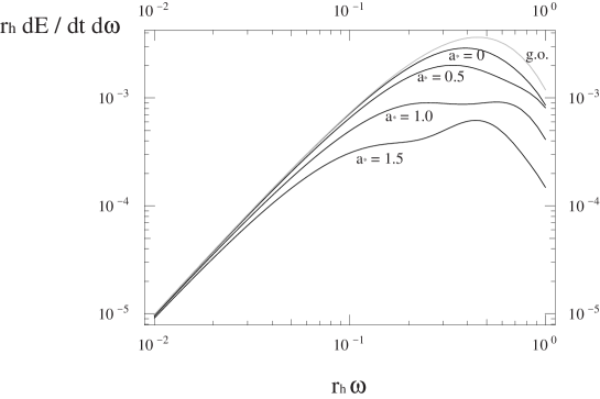
Figure 3: Scalar ($s=0$) power spectrum $r_{h}dE/dtd\omega$ vs. $r_{h}\omega$ in log-log plot. See the caption of Fig. 2 for explantion.

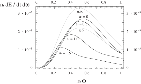
Figure 4: Spinor ($s=1/2$) power spectrum $r_{h}dE/dtd\omega$ vs. $\widetilde{\omega}=r_{h}\omega$ in linear-linear plot. Two gray lines below and above correspond to the geometrical optics limit with and without the phenomenological weighting factor 2/3, respectively. The black lines are our results for $a_{*}=0$, $0.5$, $1.0$ and $1.5$, respectively from right to left at the peak location. Note that our approximation is valid for $\widetilde{\omega}<\min(1,a_{*}^{-1})$.

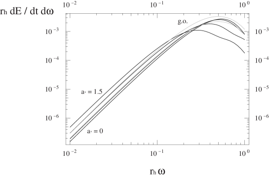
Figure 5: Spinor ($s=1/2$) power spectrum $r_{h}dE/dtd\omega$ vs. $r_{h}\omega$ in log-log plot. See the caption of Fig. 4 for explantion.

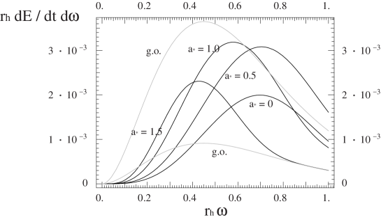
Figure 6: Vector ($s=1$) power spectrum $r_{h}dE/dtd\omega$ vs. $\widetilde{\omega}=r_{h}\omega$ in linear-linear plot. Two gray lines below and above correspond to the geometrical optics limit with and without the phenomenological weighting factor 1/4, respectively. The black lines are our results for $a_{*}=0$, $0.5$, $1.0$ and $1.5$, respectively from below to above at the left of the peaks. Note that our approximation is valid for $\widetilde{\omega}<\min(1,a_{*}^{-1})$.

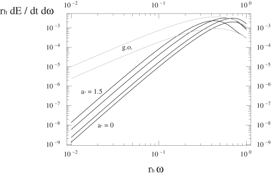
Figure 7: Vector ($s=1$) power spectrum $r_{h}dE/dtd\omega$ vs. $r_{h}\omega$ in log-log plot. See the caption of Fig. 6 for explantion.

In Figs. 2–7, we show the power spectrum (71) for spin 0, 1/2 and 1 fields. The black lines are our results for $a_{*}=0$, $0.5$, $1.0$ and $1.5$ utilizing the expression (95) with up to $l\leq 7$ modes, respectively from below to above at the left of the peak (and from above to below at the right of the peak). Note that our approximation is valid for the region satisfying both of $a_{*}\widetilde{\omega}<1$ and $\widetilde{\omega}<1$, typically at the left of the peak. Two gray lines below and above are the corresponding power spectra in the geometrical optics limit (79) with and without phenomenological weighting factor, respectively (2/3 for spinors or 1/4 for vectors) [13, 14].

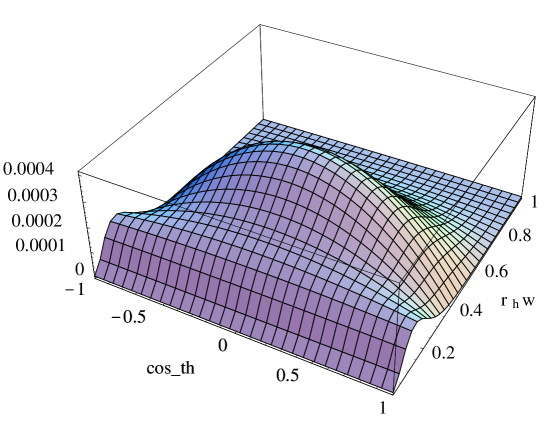
Figure 8: Scalar ($s=0$) power spectrum $r_{h}dE/dtd\omega d\cos\vartheta$ vs. $r_{h}\omega$ and $\cos\vartheta$ for $a_{*}=1.5$.

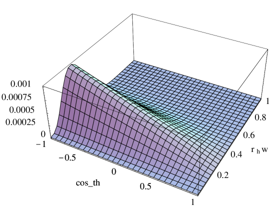
Figure 9: Spinor ($s=1/2$) power spectrum $r_{h}dE/dtd\omega d\cos\vartheta$ vs. $r_{h}\omega$ and $\cos\vartheta$ for $a_{*}=1.5$.

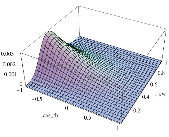
Figure 10: Vector ($s=1$) power spectrum $r_{h}dE/dtd\omega d\cos\vartheta$ vs. $r_{h}\omega$ and $\cos\vartheta$ for $a_{*}=1.5$.

In Figs. 8–10, we present the angular dependent power spectrum (72) for spin 0, 1/2 and 1 fields when $a_{*}=(a_{*})_{\mathrm{max}}=1.5$. The modes are taken up to $l\leq 1$. We observe that there is large angular dependence for spinors and vectors. Note that $\vartheta=0$ corresponds the direction of the angular momentum of the black hole which is perpendicular to the beam axis. The angular dependence shown in Figs. 8–10 vanishes when we take the limit $a_{*}\rightarrow 0$.

4 Summary

We have studied theoretical aspects of the rotating black hole production and evaporation.

For production, we present an estimation of the geometrical cross section up to unknown mass and angular momentum loss in the balding phase. Our result of the maximum impact parameter $b_{\mathrm{max}}$ is in good agreement with the numerical result by Yoshino and Nambu when the number of extra dimensions is $n\geq 1$ (i.e. within 6.5% when $n=1$ and 1.5% when $n\geq 2$), though ours predicts same as the naive value in the Schwarzschild approximation $b_{\mathrm{max}}=r_{S}(M)$ when $n=0$ which is 24% larger than the numerical result. (Here we note that our refinement from the Schwarzschild approximation results in the enlargement of the production cross section, contrary to the previous claim in the literature.) Relying on this agreement, we obtain the (differential) cross section for a given mass and (an interval of) an angular momentum, which increases linearly with the angular momentum up to the cut-off value $J_{\mathrm{max}}=b_{\mathrm{max}}M/2$. This result shows that black holes tend to be produced with large angular momenta. We also studied the possibility of the black ring formation and find that it would possibly form when there are many extra dimensions.

For evaporation, we first calculate the brane field equations for general spin and for an arbitrary number of extra dimensions. We show that the equations are separable into radial and angular parts as the four-dimensional Teukolsky equations. From these equations, we obtain the greybody factors for brane fields with general spin for the five-dimensions ($n=1$) Kerr black hole within the low-frequency expansion. We present the resultant power spectrum which is substantially different from the one with geometrical approximation utilized in the literature.

We address several phenomenological implications of our results. The production cross section of the black holes becomes larger than the one calculated from the Schwarzschild radius. The more precise determination of the radiation power is now available. We have shown that the black holes are produced with large angular momenta and that the resultant radiations will have strong angular dependence for $s=1/2$ and $s=1$ modes which points perpendicular to the beam axis while very small angular dependence is expected for scalar mode. When we average over opposite helicity states, the up-down asymmetry with respect to the angular momentum axis shown in Fig. 9 disappears (though there still remains angular dependence itself) [56, 57]; We expect similar result for vector fields (which correspond to Fig. 10). More quantitative estimation will need the greybody factors for arbitrary frequency calculated numerically.

Acknowledgments

We are grateful to Bob McElrath and Graham Kribs for helpful communications, and to Gungwon Kang and Manuel Drees for useful comments. D.I. would like to thank R. Emparan for discussions. D.I. was supported by JSPS Research, and this research was supported in part by the Grant-in-Aid for Scientific Research Fund (No. 6499). K.O. thanks to the members of KIAS theory group for their hospitality during the stay in April 2002 and is grateful to the International Center for Elementary Particle Physics for financial support during the main period of this work. The work of K.O. is partly supported by the SFB375 of the Deutsche Forschungsgemeinschaft.

Appendix

Appendix A Separability of brane fields

The various field equations in the four-dimensional Kerr background are known to be separable. This results from the special feature of the four-dimensional Kerr metric, that is, the vacuum metric which has a pair of degenerate principal null directions (Petrov type D). The four-dimensional metric considered in this paper is the induced metric of the totally geodesic probe brane in the higher-dimensional Kerr field. Though this brane metric turns out to be of Petrov type D, it is not the vacuum metric itself. Nevertheless, it happens that the massless fields on the brane are separable, as shown bellow.

The induced metric on the three-brane in the $(4+n)$-dimensional Kerr metric (with a single nonzero angular momentum) is given in terms of the Boyer-Lindquist coordinate system by

$$g = \left(1-{\mu\over\Sigma}r^{1-n}\right)dt^{2}+{2a\mu\over\Sigma}r^{1-n}\sin^{2}\vartheta dtd\varphi-\sin^{2}\vartheta\left(r^{2}+a^{2}+{\mu a^{2}\sin^{2}\vartheta\over\Sigma}r^{1-n}\right)d\varphi^{2}$$ (98)

$${}-{\Sigma\over\Delta}dr^{2}-{\Sigma}d\vartheta^{2},$$

where

$$\Sigma=r^{2}+a^{2}\cos^{2}\vartheta,\hskip 28.45274pt\Delta=r^{2}+a^{2}-\mu r^{1-n},$$ (99)

and the parameters $\mu$ and $a$ are equivalent to the total mass $M$ and the angular momentum $J$

$$M={(n+2)A_{n+2}\mu\over 16\pi G},\hskip 28.45274ptJ={A_{n+2}\mu a\over 8\pi G}.$$ (100)

where $A_{n+2}=2\pi^{(n+3)/2}/\Gamma((n+3)/2)$ is the area of a unit $(n+2)$-sphere.

The direct calculation shows that the massless scalar field equation separates on this background geometry. If we set $\varphi=R(r)S(\vartheta)e^{-i\omega t+im\varphi}$, then $\nabla^{2}\varphi=0$ becomes

$${1\over\sin\vartheta}{d\over d\vartheta}\left(\sin\vartheta{dS\over d\vartheta}\right)+\left(a^{2}\omega^{2}\cos^{2}\vartheta-m^{2}\csc^{2}\vartheta+A\right)S=0,$$ (101)

$${d\over dr}\left(\Delta{dR\over dr}\right)+\Biggl{[}{K^{2}\over\Delta}+4i\omega r-i{[2r+(n-1)\mu r^{-n}]K\over\Delta}$$

$${}+2ma\omega-a^{2}\omega^{2}-A\Biggl{]}R=0,$$ (102)

where $K=(r^{2}+a^{2})\omega-am$. We note that the Hamilton-Jacobi and massive scalar field equations are also separable though we do not shown them here; a test particle on the brane has an additional conserved quantity (Carter constant) besides the energy and the angular momentum.

To show the separability of higher spinor field equations, we work on the Newman-Penrose formalism [51]. We set the null tetrad as follows:

$$n_{\mu} = \delta_{\mu}^{t}-a\sin^{2}\vartheta\delta_{\mu}^{\varphi}-{\Sigma\over\Delta}\delta_{\mu}^{r},$$

$$n^{\prime}_{\mu} = {\Delta\over 2\Sigma}\left(\delta_{\mu}^{t}-a\sin^{2}\vartheta\delta_{\mu}^{\varphi}\right)+{1\over 2}\delta_{\mu}^{r},$$

$$m_{\mu} = {i\sin\vartheta\over 2^{1/2}(r+ia\cos\vartheta)}\left[a\delta_{\mu}^{t}-(r^{2}+a^{2})\delta_{\mu}^{\varphi}\right]-{r-ia\cos\vartheta\over 2^{1/2}}\delta_{\mu}^{\vartheta},$$

$$m^{\prime}_{\mu} = \bar{m}_{\mu}.$$ (103)

where the bar denotes the complex conjugation. These are subject to the normalization: $n_{\mu}n^{\prime\mu}=-m_{\mu}m^{\prime\mu}=1$, $n_{\mu}n^{\mu}=n^{\prime}_{\mu}n^{\prime\mu}=m_{\mu}m^{\mu}=n_{\mu}m^{\mu}=n^{\prime}_{\mu}m^{\mu}=0$. Alternative description is given by the two-component spinor $o^{A},\iota^{A}$ via the identification

$$(n^{\mu},n^{\prime\mu},m^{\mu},m^{\prime\mu})\leftrightarrow(o^{A}\bar{o}^{A^{\prime}},\iota^{A}\bar{\iota}^{A^{\prime}},o^{A}\bar{\iota}^{A^{\prime}},\iota^{A}\bar{o}^{A^{\prime}}),$$ (104)

with the symplectic structure $\epsilon^{AB}=o^{A}\iota^{B}-\iota^{A}o^{B}$, $\epsilon^{01}=\epsilon_{01}=1$. Each component of the spinor covariant derivative $\nabla_{AA^{\prime}}$ is denoted by

$$(\nabla_{o\bar{o}},\nabla_{\iota\bar{\iota}},\nabla_{o\bar{\iota}},\nabla_{\iota\bar{o}})=(D,D^{\prime},\delta,\delta^{\prime}),$$ (105)

and the spin-coefficients are defined by

$$D(o,\iota) = (\epsilon o-\kappa\iota,-\tau^{\prime}o-\epsilon\iota),~{}~{}~{}D^{\prime}(o,\iota)=(-\epsilon^{\prime}o-\tau\iota,-\kappa^{\prime}o+\epsilon^{\prime}\iota),$$

$$\delta(o,\iota) = (\beta o-\sigma\iota,-\rho^{\prime}o-\beta\iota),~{}~{}~{}\delta^{\prime}(o,\iota)=(-\beta^{\prime}o-\rho\iota,-\sigma^{\prime}o+\beta^{\prime}\iota).$$

Then, all the nonzero spin-coefficients are

$$\tau = -{ia\sin\vartheta\over 2^{1/2}\Sigma},~{}~{}~{}\rho=-{1\over r-ia\cos\vartheta},~{}~{}~{}\beta=-{\bar{\rho}\cot\vartheta\over 2\sqrt{2}},~{}~{}~{}\tau^{\prime}=-{ia\rho^{2}\sin\vartheta\over\sqrt{2}},$$

$$\rho^{\prime} = -{\rho^{2}\bar{\rho}\Delta\over 2},~{}~{}~{}\epsilon^{\prime}=\rho^{\prime}-{\rho\bar{\rho}\over 4}\Delta_{,r},~{}~{}~{}\beta^{\prime}=\tau^{\prime}+\bar{\beta}.$$ (107)

Here, let us consider the Weyl equation ($s=1/2$) and the Maxwell equation ($s=1$) on this background brane metric.

We define the component of the Weyl spinor $\psi_{A}$ simply by $\psi_{0}=\psi_{A}o^{A}$ and $\psi_{1}=\psi_{A}\iota^{A}$. Then, each component of the Weyl equation $\nabla^{AA^{\prime}}\psi_{A}$ becomes explicitly

$$D\psi_{1}-\delta^{\prime}\psi_{0} = (\beta^{\prime}-\tau^{\prime})\psi_{0}+(\rho-\epsilon)\psi_{1},$$ (108)

$$\delta\psi_{1}-D^{\prime}\psi_{0} = (\epsilon^{\prime}-\rho^{\prime})\psi_{0}+(\tau-\beta)\psi_{1}.$$ (109)

On the other hand, the Maxwell field is represented by the second-rank symmetric spinor $\phi_{AB}$, and its components are denoted by $\phi_{0}=\phi_{AB}o^{A}o^{B}$, $\phi_{1}=\phi_{AB}o^{A}\iota^{B}$ and $\phi_{2}=\phi_{AB}\iota^{A}\iota^{B}$, respectively. Then, the source-free Maxwell equation $\nabla^{AA^{\prime}}\phi_{AB}=0$ leads to

$$D\phi_{1}-\delta^{\prime}\phi_{0} = (2\beta^{\prime}-\tau^{\prime})\phi_{0}+2\rho\phi_{1}-\kappa\phi_{2}$$ (110)

$$D\phi_{2}-\delta^{\prime}\phi_{1} = \sigma^{\prime}\phi_{0}-2\tau^{\prime}\phi_{1}+(\rho-2\epsilon)\phi_{2}$$ (111)

$$D^{\prime}\phi_{0}-\delta\phi_{1} = (\rho^{\prime}-2\epsilon^{\prime})\phi_{0}-2\tau\phi_{1}+\sigma\phi_{2}$$ (112)

$$D^{\prime}\phi_{1}-\delta\phi_{2} = -\kappa^{\prime}\phi_{0}+2\rho^{\prime}\phi_{1}+(2\beta-\tau)\phi_{2}.$$ (113)

The brane-induced metric turns out to be of Petrov type D, namely, the gravitational spinor $\Psi_{ABCD}$ has only nonzero component $\Psi_{2}$$=$$\Psi_{ABCD}o^{A}o^{B}\iota^{C}\iota^{D}$. Besides this condition, when $\kappa=\sigma=\kappa^{\prime}=\sigma^{\prime}=0$ hold as in the present case, we have the identities for the differential operators

$$[D-(p+1)\epsilon+\bar{\epsilon}+q\rho-\bar{\rho}](\delta-p\beta+q\tau)$$

$${}-[\delta-(p+1)\beta+\bar{\beta}^{\prime}-\bar{\tau}^{\prime}+q\tau](D-p\epsilon+q\rho)=0,$$ (114)

$$[D^{\prime}-(p+1)\epsilon^{\prime}+\bar{\epsilon}^{\prime}+q\rho^{\prime}-\bar{\rho}^{\prime}](\delta^{\prime}-p\beta^{\prime}+q\tau^{\prime})$$

$${}-[\delta^{\prime}-(p+1)\beta^{\prime}+\bar{\beta}-\bar{\tau}+q\tau^{\prime}](D^{\prime}-p\epsilon^{\prime}+q\rho^{\prime})=0,$$ (115)

for any pair of the numbers ($p,q$), where we have used the identities

$$\delta D-D\delta = (\bar{\tau^{\prime}}-\bar{\beta^{\prime}}+\beta)D+\kappa D^{\prime}-(\bar{\rho}+\epsilon-\bar{\epsilon})\delta-\sigma\delta^{\prime},$$ (116)

$$\delta^{\prime}D^{\prime}-D^{\prime}\delta^{\prime} = \kappa^{\prime}D+(\bar{\tau}-\bar{\beta}+\beta^{\prime})D^{\prime}-\sigma^{\prime}\delta-(\bar{\rho^{\prime}}+\epsilon^{\prime}-\bar{\epsilon^{\prime}})\delta^{\prime}.$$ (117)

Applying $(\delta+\bar{\beta}^{\prime}-\bar{\tau}^{\prime}-\tau)$ to Eq. (108) and $(D+\bar{\epsilon}-\rho-\bar{\rho})$ to Eq. (109), subtracting one from the other, and using Eq. (114) for $(p,q)=(-1,-1)$, we obtain the decoupled equation for $\psi_{0}$

$$\Biggl{\{}\left[{(r^{2}+a^{2})^{2}\over\Delta}-a^{2}\sin^{2}\vartheta\right]{\partial^{2}\over\partial t^{2}}+2a\left({r^{2}+a^{2}\over\Delta}-1\right){\partial^{2}\over\partial t\partial\varphi}+\left({a^{2}\over\Delta}-{1\over\sin^{2}\vartheta}\right){\partial^{2}\over\partial\varphi^{2}}$$

$${}+\left[2r-{(r^{2}+a^{2})\Delta_{,r}\over 2\Delta}+ia\cos\vartheta\right]{\partial\over\partial t}+\left[-{a\Delta_{,r}\over 2\Delta}-{i\cos\vartheta\over\sin^{2}\vartheta}\right]{\partial\over\partial\varphi}$$

$${}-\Delta^{-1/2}{\partial\over\partial r}\Delta^{3/2}{\partial\over\partial r}-{1\over\sin\vartheta}{\partial\over\partial\vartheta}\sin\vartheta{\partial\over\partial\vartheta}+{\cot^{2}\vartheta\over 4}-{1\over 2}+{n(n-1)\mu r^{-n-1}\over 2}\Biggr{\}}\psi_{0}=0.$$

If we set $\psi_{0}=R(r)S(\vartheta)e^{-i\omega t+im\varphi}$, then we obtain

$${1\over\sin\vartheta}{d\over d\vartheta}\left(\sin\vartheta{dS\over d\vartheta}\right)$$

$${}+\left(a^{2}\omega^{2}\cos^{2}\vartheta-{m^{2}\over\sin^{2}\vartheta}-a\omega\cos\vartheta-{m\cos\vartheta\over\sin^{2}\vartheta}-{1\over 4}\cot^{2}\vartheta+{1\over 2}+A\right)S=0,$$

(119)

$$\Delta^{-1/2}{d\over dr}\left(\Delta^{3/2}{dR\over dr}\right)$$

$${}+\Biggl{[}\left({K^{2}\over\Delta}+2i\omega r-{i\over 2}{[2r+(n-1)\mu r^{-n}]K\over\Delta}\right)$$

$${}-{n(n-1)\mu r^{-n-1}\over 2}+2ma\omega-a^{2}\omega^{2}-A\Biggl{]}R=0.$$ (120)

For the Maxwell field, applying $(\delta-\beta+\bar{\beta}^{\prime}-\bar{\tau}^{\prime}-2\tau)$ to Eq. (110) and $(D-\epsilon+\bar{\epsilon}-2\rho-\bar{\rho})$ to Eq. (111), subtracting one from the other, and using Eq. (114) for $(p,q)=(0,-2)$, we obtain

$$\Biggl{\{}\left[{(r^{2}+a^{2})^{2}\over\Delta}-a^{2}\sin^{2}\vartheta\right]{\partial^{2}\over\partial t^{2}}+\left[{2a(r^{2}+a^{2})\over\Delta}-2a\right]{\partial^{2}\over\partial t\partial\varphi}+\left[{a^{2}\over\Delta}-{1\over\sin^{2}\vartheta}\right]{\partial^{2}\over\partial\varphi^{2}}$$

$${}+\left[-{\mu r^{-n}\left[(n+1)r^{2}+(n-1)a^{2}\right]\over\Delta}+2(r+ia\cos\vartheta)\right]{\partial\over\partial t}$$

$${}+\left[-{a[2r+(n-1)\mu r^{-n}]\over\Delta}-{2i\cos\vartheta\over\sin^{2}\vartheta}\right]{\partial\over\partial\varphi}$$

$${}-{1\over\Delta}{\partial\over\partial r}\Delta^{2}{\partial\over\partial r}-{1\over\sin\vartheta}{\partial\over\partial\vartheta}\sin\vartheta{\partial\over\partial\vartheta}+\cot^{2}\vartheta-1+n(n-1)\mu r^{-n-1}\Biggr{\}}\varphi_{0}=0.$$

Set $\phi_{0}=R(r)S(\vartheta)e^{-i\omega t+im\varphi}$, then we have

$${1\over\sin\vartheta}{d\over d\vartheta}\left(\sin\vartheta{dS\over d\vartheta}\right)$$

$${}+\left(a^{2}\omega^{2}\cos^{2}\vartheta-{m^{2}\over\sin^{2}\vartheta}-2a\omega\cos\vartheta-{2m\cos\vartheta\over\sin^{2}\vartheta}-\cot^{2}\vartheta+1+A\right)S=0,$$

(122)

$${1\over\Delta}{d\over dr}\left(\Delta^{2}{dR\over dr}\right)$$

$${}+\Biggl{[}{K^{2}\over\Delta}+4i\omega r-i{[2r+(n-1)\mu r^{-n}]K\over\Delta}$$

$${}-n(n-1)\mu r^{-n-1}+2ma\omega-a^{2}\omega^{2}-A\Biggl{]}R=0.$$ (123)

In summary, the spin-$s$ massless field equation becomes

$${1\over\sin\vartheta}{d\over d\vartheta}\left(\sin\vartheta{dS\over d\vartheta}\right)$$

$${}+\left[(s-a\omega\cos\vartheta)^{2}-(s\cot\vartheta+m\csc\vartheta)^{2}-s(s-1)+A\right]S=0,$$

and

$$\Delta^{-s}{d\over dr}\left(\Delta^{s+1}{dR\over dr}\right)+\Biggl{[}{K^{2}\over\Delta}+s\left(4i\omega r-i{[2r+(n-1)\mu r^{-n}]K\over\Delta}-n(n-1)\mu r^{-n-1}\right)$$

$${}+2ma\omega-a^{2}\omega^{2}-A\Biggl{]}R=0.$$ (125)

Figure 2: Scalar ($s=0$) power spectrum $r_{h}dE/dtd\omega$ vs. $\widetilde{\omega}=r_{h}\omega$ in lenear-linear plot. The gray line corresponds the geometrical optics limit. The black lines are our results for $a_{*}=0$, $0.5$, $1.0$ and $1.5$ from above to below. Note that our approximation is valid for $\widetilde{\omega}<\min(1,a_{*}^{-1})$.

References

• [1] N. Arkani-Hamed, S. Dimopoulos, and G. R. Dvali, “The hierarchy problem and new dimensions at a millimeter,” Phys. Lett. B429 (1998) 263–272, hep-ph/9803315.
• [2] I. Antoniadis, N. Arkani-Hamed, S. Dimopoulos, and G. R. Dvali, “New dimensions at a millimeter to a fermi and superstrings at a TeV,” Phys. Lett. B436 (1998) 257–263, hep-ph/9804398.
• [3] L. J. Hall and D. R. Smith, “Cosmological constraints on theories with large extra dimensions,” Phys. Rev. D60 (1999) 085008, hep-ph/9904267.
• [4] L. Randall and R. Sundrum, “A large mass hierarchy from a small extra dimension,” Phys. Rev. Lett. 83 (1999) 3370–3373, hep-ph/9905221.
• [5] T. Banks and W. Fischler, “A model for high energy scattering in quantum gravity,” hep-th/9906038.
• [6] R. Emparan, G. T. Horowitz, and R. C. Myers, “Black holes radiate mainly on the brane,” Phys. Rev. Lett. 85 (2000) 499–502, hep-th/0003118.
• [7] S. B. Giddings and S. Thomas, “High energy colliders as black hole factories: The end of short distance physics,” Phys. Rev. D65 (2002) 056010, hep-ph/0106219.
• [8] S. Dimopoulos and G. Landsberg, “Black holes at the LHC,” Phys. Rev. Lett. 87 (2001) 161602, hep-ph/0106295.
• [9] P. C. Argyres, S. Dimopoulos, and J. March-Russell, “Black holes and sub-millimeter dimensions,” Phys. Lett. B441 (1998) 96–104, hep-th/9808138.
• [10] J. L. Feng and A. D. Shapere, Phys. Rev. Lett. 88, 021303 (2002); L. Anchordoqui and H. Goldberg, Phys. Rev. D 65, 047502 (2002); R. Emparan, M. Masip and R. Rattazzi, Phys. Rev. D 65, 064023 (2002); Y. Uehara, Prog. Theor. Phys. 107, 621 (2002); A. Ringwald and H. Tu, Phys. Lett. B 525, 135 (2002); L. A. Anchordoqui, J. L. Feng, H. Goldberg and A. D. Shapere, Phys. Rev. D 65, 124027 (2002); M. Kowalski, A. Ringwald and H. Tu, Phys. Lett. B 529, 1 (2002); P. Jain, S. Kar, S. Panda and J. P. Ralston, hep-ph/0201232; J. Alvarez-Muniz, J. L. Feng, F. Halzen, T. Han and D. Hooper, Phys. Rev. D 65, 124015 (2002); L. A. Anchordoqui, J. L. Feng and H. Goldberg, Phys. Lett. B 535, 302 (2002); S. I. Dutta, M. H. Reno and I. Sarcevic, Phys. Rev. D 66, 033002 (2002); H. Goldberg and A. D. Shapere, P. Jain, S. Kar, D. W. McKay, S. Panda and J. P. Ralston, Phys. Rev. D 66, 065018 (2002); P. Gorham, J. Learned and N. Lehtinen, astro-ph/0205170; L. A. Anchordoqui, J. L. Feng, H. Goldberg and A. D. Shapere, hep-ph/0207139.
• [11] L. A. Anchordoqui, H. Goldberg, and A. D. Shapere, “Phenomenology of Randall-Sundrum black holes,” Phys. Rev. D66 (2002) 024033, hep-ph/0204228.
• [12] K. Cheung, Phys. Rev. Lett. 88, 221602 (2002); Phys. Rev. D 66, 036007 (2002); A. Ringwald and H. Tu, Phys. Lett. B 525, 135 (2002); S. Hofmann, M. Bleicher, L. Gerland, S. Hossenfelder, S. Schwabe and H. Stocker, hep-ph/0111052; T. G. Rizzo, hep-ph/0111230; JHEP 0202, 011 (2002); G. Landsberg, Phys. Rev. Lett. 88, 181801 (2002); M. Bleicher, S. Hofmann, S. Hossenfelder and H. Stocker, Phys. Lett. 548, 73 (2002); Y. Uehara, hep-ph/0205122; hep-ph/0205199; K. Cheung and C. H. Chou, Phys. Rev. D 66, 036008 (2002); A. Chamblin and G. C. Nayak, hep-ph/0206060.
• [13] T. Han, G. D. Kribs, and B. McElrath, “Black hole evaporation with separated fermions,” hep-ph/0207003.
• [14] L. Anchordoqui and H. Goldberg, “Black hole chromosphere at the LHC,” hep-ph/0209337.
• [15] M. B. Voloshin, “Semiclassical suppression of black hole production in particle collisions,” Phys. Lett. B518 (2001) 137–142, hep-ph/0107119.
• [16] S. B. Giddings, “Black hole production in TeV-scale gravity, and the future of high energy physics,” hep-ph/0110127.
• [17] M. B. Voloshin, “More remarks on suppression of large black hole production in particle collisions,” Phys. Lett. B524 (2002) 376–382, hep-ph/0111099.
• [18] D. M. Eardley and S. B. Giddings, “Classical black hole production in high-energy collisions,” Phys. Rev. D66 (2002) 044011, gr-qc/0201034.
• [19] E. Kohlprath and G. Veneziano, “Black holes from high-energy beam-beam collisions,” JHEP 06 (2002) 057, gr-qc/0203093.
• [20] H. Yoshino and Y. Nambu, “Black hole formation in the grazing collision of high- energy particles,” gr-qc/0209003.
• [21] S. Dimopoulos and R. Emparan, “String balls at the LHC and beyond,” Phys. Lett. B526 (2002) 393–398, hep-ph/0108060.
• [22] G.-w. Kang and K.-y. Oda. unpublished.
• [23] K.-y. Oda and N. Okada, “Alternative signature of TeV strings,” Phys. Rev. D66 (2002) 095005, hep-ph/0111298.
• [24] S. W. Hawking, “Particle creation by black holes,” Commun. Math. Phys. 43 (1975) 199–220.
• [25] J. Polchinski, “String duality: A colloquium,” Rev. Mod. Phys. 68 (1996) 1245–1258, hep-th/9607050.
• [26] G. T. Horowitz and J. Polchinski, “A correspondence principle for black holes and strings,” Phys. Rev. D55 (1997) 6189–6197, hep-th/9612146.
• [27] R. C. Myers and M. J. Perry, “Black holes in higher dimensional space-times,” Ann. Phys. 172 (1986) 304.
• [28] S. B. Giddings, E. Katz, and L. Randall, “Linearized gravity in brane backgrounds,” JHEP 03 (2000) 023, hep-th/0002091.
• [29] S. B. Giddings and E. Katz, “Effective theories and black hole production in warped compactifications,” J. Math. Phys. 42 (2001) 3082–3102, hep-th/0009176.
• [30] N. Arkani-Hamed, M. Porrati, and L. Randall, “Holography and phenomenology,” JHEP 08 (2001) 017, hep-th/0012148.
• [31] D. N. Page, “Particle emission rates from a black hole: Massless particles from an uncharged, nonrotating hole,” Phys. Rev. D13 (1976) 198–206.
• [32] D. N. Page, “Particle emission rates from a black hole. II. Massless particles from a rotating hole,” Phys. Rev. D14 (1976) 3260–3273.
• [33] A. V. Kotwal and C. Hays, “Production and decay of spinning black holes at colliders and tests of black hole dynamics,” hep-ph/0206055.
• [34] S. C. Park and H. S. Song, “Production of spinning black holes at colliders,” hep-ph/0111069.
• [35] S. N. Solodukhin, “Classical and quantum cross-section for black hole production in particle collisions,” Phys. Lett. B533 (2002) 153–161, hep-ph/0201248.
• [36] S. D. H. Hsu, “Quantum production of black holes,” hep-ph/0203154.
• [37] A. A. Starobinsky, “Amplification of waves during reflection from a rotating black hole,” Sov. Phys. JETP 37 (1973) 28–32.
• [38] S. A. Teukolsky, “Rotating black holes: Separable wave equations for gravitational and electromagnetic perturbations,” Phys. Rev. Lett. 29 (1972) 1114–1118.
• [39] A. A. Starobinsky and S. M. Churilov, “Amplification of electromagnetic and gravitational waves scattered by a rotating black hole,” Sov. Phys. JETP 38 (1974) 1–5.
• [40] S. A. Teukolsky, “Perturbations of a rotating black hole. I. Fundamental equations for gravitational, electromagnetic, and neutrino-field perturbations,” Astrophys. J. 185 (1973) 635–647.
• [41] W. H. Press and S. A. Teukolsky, “Perturbations of a rotating black hole. II. Dynamical stability of the Kerr metric,” Astrophys. J. 185 (1973) 649–674.
• [42] S. A. Teukolsky and W. H. Press, “Perturbations of a rotating black hole. III. Interaction of the hole with gravitational and electromagnetic radiation,” Astrophys. J. 193 (1974) 443–461.
• [43] P. Kanti and J. March-Russell, “Calculable corrections to brane black hole decay. I: The scalar case,” Phys. Rev. D66 (2002) 024023, hep-ph/0203223.
• [44] V. Cardoso and J. P. S. Lemos, “Gravitational radiation from collisions at the speed of light: A massless particle falling into a Schwarzschild black hole,” Phys. Lett. B538 (2002) 1–5, gr-qc/0202019.
• [45] V. Cardoso and J. P. S. Lemos, “The radial infall of a highly relativistic point particle into a Kerr black hole along the symmetry axis,” gr-qc/0207009.
• [46] V. Cardoso and J. P. S. Lemos, “Gravitational radiation from the radial infall of highly relativistic point particles into Kerr black holes,” gr-qc/0211094.
• [47] M.-l. Cai and G. J. Galloway, “On the topology and area of higher dimensional black holes,” Class. Quant. Grav. 18 (2001) 2707–2718, hep-th/0102149.
• [48] R. Emparan and H. S. Reall, “A rotating black ring in five dimensions,” Phys. Rev. Lett. 88 (2002) 101101, hep-th/0110260.
• [49] V. Frolov and D. Stojkovic, “Black hole radiation in the brane world and recoil effect,” Phys. Rev. D66 (2002) 084002, hep-th/0206046.
• [50] V. Frolov and D. Stojkovic, “Black hole as a point radiator and recoil effect on the brane world,” Phys. Rev. Lett 89 (2002) 151302, hep-th/0208102.
• [51] E. Newman and R. Penrose, “An approach to gravitational radiation by a method of spin coefficients,” J. Math. Phys. 3 (1962) 566–578.
• [52] E. D. Fackerell and R. G. Crossman, “Spin-weighted angular spheroidal functions,” J. Math. Phys. 18 (1977) 1849–1854.
• [53] J. N. Goldberg, A. J. MacFarlane, E. T. Newman, F. Rohrlich, and E. C. G. Sudarshan, “Spin s spherical harmonics and edth,” J. Math. Phys. 8 (1967) 2155–2161.
• [54] D. Ida, K.-y. Oda, and S. C. Park. in progress.
• [55] V. Frolov and D. Stojkovic, “Quantum radiation from a 5-dimensional rotating black hole,” gr-qc/0211055.
• [56] A. Vilenkin, “Parity nonconservation and rotating black holes,” Phys. Rev. Lett. 41 (1978) 1575–1577.
• [57] D. A. Leahy and W. G. Unruh, “Angular dependence of neutrino emission from rotating black holes,” Phys. Rev. D19 (1979) 3509–3515.
• [58] R. Penrose and W. Rindler, “Spinors and space-time. 1. two spinor calculus and relativistic fields,”. Cambridge, UK: Univ. Pr. (1984) 458 P. (Cambridge Monographs On Mathematical Physics).
Refer to caption