Toward Solving the Cosmological Constant Problem?

Abstract

We discuss the cosmological constant problem in the context of higher codimension brane world scenarios with infinite-volume extra dimensions. In particular, by adding higher curvature terms in the bulk action we are able to find smooth solutions with the property that the 4-dimensional part of the brane world-volume is flat for a range of positive values of the brane tension.

I Introduction and Summary

As was proposed in [1], one can reproduce four-dimensional gravity on a 3-brane in 6 or higher dimensional infinite-volume bulk if one includes the Einstein-Hilbert term on the brane (the latter is induced at the quantum level if the brane matter is non-conformal). Gravity then is almost completely localized on the brane with only ultra-light modes penetrating into the bulk, so that gravity is four-dimensional at distance scales up to an ultra-large cross-over scale $r_{c}$ (beyond which gravity becomes higher dimensional), which can be larger than the present Hubble size. In particular, this is the case for codimension-2 and higher tensionless branes [1] as well as for codimension-2 non-zero tension branes [2]. This is also expected to be the case for codimension-3 and higher non-zero tension branes [3, 4].

A careful analysis of linearized gravity in such backgrounds requires smoothing out higher codimension singularities [1, 3]. This is already the case for tensionless branes, where the background is non-singular (in fact, it is flat), but the graviton propagator is singular. However, as was pointed out in [4], these singularities in the graviton propagator are cured once we include higher curvature terms on the brane. These terms are induced at the quantum level along with the Einstein-Hilbert term, and provide an ultra-violet cut-off for the graviton propagator. In the presence of these terms, to reproduce four-dimensional gravity up to the present Hubble size, we need to assume that the bulk Planck scale $M_{P}{\ \lower-1.2pt\vbox{\hbox{\hbox to0.0pt{$<$\hss}\lower 5.0pt\vbox{\hbox{$\sim$}}}}\ }(1~{}{\rm mm})^{-1}$ regardless of the codimension of the brane (assuming that it is 2 or higher) [4].

In the case of non-zero tension branes, however, the situation is more complicated as in the case of $\delta$-function-like branes the background itself becomes singular (for phenomenologically interesting non-BPS branes on which we focus in this paper). More precisely, here we focus on solutions with vanishing cosmological constant on the brane. Then in the codimension-2 case the singularity is very mild as in the extra 2 dimensions the background has the form of a wedge with a deficit angle, so the singularity is a simple conical one [2]. As was discussed in [3], this singularity can be consistently smoothed out. In this case gravity on the brane was analyzed in [2, 3], where it was found that the behavior of gravity is essentially unmodified compared with the tensionless brane cases. In particular, gravity is almost completely localized with only ultra-light modes penetrating into the bulk, and four-dimensional gravity on the brane can be reproduced up to distance scales of order of the current Hubble size. As to the brane tension, in codimension-2 solutions with vanishing brane cosmological constant it can take continuous values in the range bounded below by zero and bounded above by its critical value [2], which is of order $M_{P}^{4}{\ \lower-1.2pt\vbox{\hbox{\hbox to0.0pt{$<$\hss}\lower 5.0pt\vbox{\hbox{$\sim$}}}}\ }(1~{}{\rm mm})^{-4}$ (for a 3-brane). Since this does not improve the current experimental bound on the 4-dimensional cosmological constant, we are prompted to consider codimension-3 and higher solutions.

In codimension-3 and higher cases with non-zero tension branes the singularities in the background itself are more severe. Actually, there are two types of singularities we must distinguish here. Thus, we can have a singularity at the origin $r=0$ of the extra space, that is, at the location of the brane. These singularities can sometimes be simple coordinate singularities, in which case they are harmless. On the other hand, true $r=0$ singularities can be smoothed out using a procedure discussed in [3]. This procedure goes as follows. Consider a codimension-$d$ ($d>2$) $\delta$-function-like source brane in $D$-dimensional bulk. Let the bulk action simply be the $D$-dimensional Einstein-Hilbert action, while on the brane we have the induced $(D-d)$-dimensional Einstein-Hilbert term as well as the cosmological term corresponding to the brane tension. As we have already mentioned, the background in this case is singular [5]. One way to smooth out such a singularity is to replace the $(D-d)$-dimensional world-volume of the brane by its product with a $d$-dimensional ball ${\bf B}_{d}$ of some non-zero radius $\epsilon$. As was pointed out in [3], in this case already for a tensionless brane the gravitational modes on the brane contain an infinite tower of tachyonic modes. This can be circumvented by considering a partial smoothing out where one replaces the $(D-d)$-dimensional world-volume of the brane by its product with a $(d-1)$-sphere ${\bf S}^{d-1}$ of radius $\epsilon$ [3]. As was pointed out in [3], this suffices for smoothing out higher codimension singularities in the graviton propagator as in the codimension-1 case the propagator is non-singular [6]. Moreover, in the case of tensionless branes as well as in the case of a non-zero tension codimension-2 brane we then have only one tachyonic mode (with ultra-low $-m^{2}$) which is expected to be an artifact of not including non-local operators on the brane. As to the background itself, this procedure does smooth out $r=0$ singularities. However, not surprisingly, it does not suffice for smoothing out the second type of singularities [7] (such singularities are absent in the codimension-2 case but are present in higher codimension cases with non-zero brane tension), which we discuss next.

Thus, in codimension-3 and higher cases with vanishing brane cosmological constant we can have singularities at $r=r_{*}$ with some non-vanishing $r_{*}$, which depends on the brane tension [5]. The aforementioned smoothing out procedure does not cure such singularities. In [7] it was suggested that higher curvature terms in the bulk might be responsible for curing such singularities. The purpose of this paper is precisely to study effects of higher curvature terms in the bulk on such singularities.

Not surprisingly, studying such backgrounds in the presence of higher curvature terms in the bulk is rather non-trivial. To make the problem more tractable, we focus on a special kind of higher curvature terms in the bulk. In particular, we consider adding the second-order (in curvature) Gauss-Bonnet combination in the bulk. This Gauss-Bonnet combination is an Euler invariant in four dimensions. In higher dimensions, however, it has a non-trivial effect on the equations of motion if the background is not flat. A simplifying feature of the Gauss-Bonnet combination is that it does not introduce terms with third and fourth derivatives in the background equations of motions, but rather makes them even more non-linear. Albeit non-trivial, these equations can in certain cases be analyzed analytically, so we can get some insight into the effect of higher curvature terms on the aforementioned $r=r_{*}$ singularities.

The results of our analyses, which we present in the remainder of this paper, suggest that higher curvature terms in the bulk might indeed cure these singularities. To simplify our discussion, as far as explicit computations are concerned, we focus on codimension-3 cases, where we have additional simplifications in the equations of motion (higher codimension cases are not expected to be qualitatively different). In particular, we explicitly study examples of: a string in 5D bulk, a membrane in 6D bulk as well as a 3-brane in 7D bulk. In these cases we argue that smooth solutions with vanishing brane cosmological constant do exist for a continuous range of positive brane tension. In the remainder of this paper, following the terminology adopted in [8], we refer to such solutions as diluting solutions.

Before we turn to a detailed description of our solutions, let us describe the geometry of the aforementioned diluting solution corresponding to a 3-brane in 7D bulk. In the extra three dimensions we have a radially symmetric solution where a 2-sphere is fibered over a semi-infinite line $[r_{0},\infty)$. The space is curved for $r_{0}\leq r<\epsilon$, at $r=\epsilon$ we have a jump in the radial derivatives of the warp factors (because $r=\epsilon$ is where the brane tension is localized), and for $r>\epsilon$ the space is actually flat. So an outside observer located at $r>\epsilon$ thinks that the brane is tensionless, while an observer inside of the sphere, that is, at $r<\epsilon$ sees the space highly curved. It would take this observer infinite time to reach the point $r=r_{0}$, where we have a coordinate singularity (that is, the corresponding geodesics are complete, so this is not a naked singularity but a coordinate one). This is an important point, in particular, we did not find smooth solutions where the space would be curved outside but flat inside of the sphere. And this is just as well. Indeed, as was shown in [7], if we have only the Einstein-Hilbert term in the bulk, then we have no smooth solutions whatsoever (that is, smoothing out the 3-brane by making it into a 5-brane with two dimensions curled up into a 2-sphere does not suffice). What is different in our solutions is that we have added higher curvature terms in the bulk, which we expected to smooth out some singularities. But serving as an ultra-violet cut-off higher curvature terms could only possibly smooth out a real singularity at $r<\epsilon$, not at $r>\epsilon$. And this is precisely what happens in our solution - the presence of higher curvature terms ensures that we have only a coordinate singularity at $r<\epsilon$ instead of a real naked singularity as would be the case had we included only the Einstein-Hilbert term.

II Setup

The brane world model we study in this paper is described by the following action:

$$S= {\widetilde{M}}^{D-3}_{P}\int_{\Sigma}d^{D-1}x~{}\sqrt{-{\widetilde{G}}}\left[{\widetilde{R}}-{\widetilde{\Lambda}}\right]+$$ (2)

$${M}^{D-2}_{P}\int d^{D}x~{}\sqrt{-{G}}~{}\left[{R}~{}+\xi\biggl{(}R^{2}-4R_{MN}^{2}+R_{MNPR}^{2}\biggl{)}\right].$$

Here $M_{P}$ is the (reduced) $D-$dimensional Planck mass, while ${\widetilde{M}}_{P}$ is the (reduced) $(D-1)$-dimensional Planck mass; $\Sigma$ is a source brane, whose geometry is given by the product ${\bf R}^{D-d-1,1}\times{\bf S}^{d-1}_{\epsilon}$, where ${\bf R}^{D-d-1,1}$ is the $(D-d)$-dimensional Minkowski space, and ${\bf S}^{d-1}_{\epsilon}$ is a $(d-1)$-sphere of radius $\epsilon$ (in the following we will assume that $d\geq 3$). The quantity ${\widetilde{M}}^{D-1}_{P}{\widetilde{\Lambda}}$ plays the role of the tension of the brane $\Sigma$. Also,

$${\widetilde{G}}_{mn}\equiv{\delta_{m}}^{M}{\delta_{n}}^{N}G_{MN}\Big{|}_{\Sigma}~{},$$ (3)

where $x^{m}$ are the $(D-1)$ coordinates along the brane (the $D$-dimensional coordinates are given by $x^{M}=(x^{m},r)$, where $r\geq 0$ is a non-compact radial coordinate transverse to the brane, and the signature of the $D$-dimensional metric is $(-,+,\dots,+)$); finally, the $(D-1)$-dimensional Ricci scalar ${\widetilde{R}}$ is constructed from the $(D-1)$-dimensional metric ${\widetilde{G}}_{\mu\nu}$. In the following we will use the notation $x^{i}=(x^{\alpha},r)$, where $x^{\alpha}$ are the $(d-1)$ angular coordinates on the sphere ${\bf S}^{d-1}_{\epsilon}$. Moreover, the metric for the coordinates $x^{i}$ will be (conformally) flat:

$$\delta_{ij}~{}dx^{i}dx^{j}=dr^{2}+r^{2}\gamma_{\alpha\beta}~{}dx^{\alpha}dx^{\beta}~{},$$ (4)

where $\gamma_{\alpha\beta}$ is the metric on a unit $(d-1)$-sphere. Also, we will denote the $(D-d)$ Minkowski coordinates on ${\bf R}^{D-d-1,1}$ via $x^{\mu}$ (note that $x^{m}=(x^{\mu},x^{\alpha})$).

The equations of motion read

$$R_{MN}-\frac{1}{2}G_{MN}R+\xi\left[2\Xi_{MN}-{1\over 2}G_{MN}\,\Xi\right]+$$ (5)

$$\displaystyle{{\sqrt{-{\widetilde{G}}}\over\sqrt{-G}}}{\delta_{M}}^{m}{\delta_{N}}^{n}\left[{\widetilde{R}}_{mn}-{1\over 2}{\widetilde{G}}_{mn}\left({\widetilde{R}}-{\widetilde{\Lambda}}\right)\right]{\widetilde{L}}~{}\delta(r-\epsilon)=0~{},$$ (6)

where $\Xi\equiv{\Xi_{M}}^{M}$, and

$$\Xi_{MN}\equiv RR_{MN}-2R_{MS}R^{S}{}_{N}+R_{MRST}R_{N}{}^{RST}-2R^{RS}R_{MRNS}~{},$$ (7)

$${\widetilde{L}}\equiv{\widetilde{M}}_{P}^{D-3}/M_{P}^{D-2}~{}.$$ (8)

Here we are interested in solutions with vanishing $(D-d)$-dimensional cosmological constant, which, at the same time, are radially symmetric in the extra $d$ dimensions. The corresponding ansatz for the background metric reads:

$$ds^{2}=\exp(2A)~{}\eta_{\mu\nu}~{}dx^{\mu}dx^{\nu}+\exp(2B)~{}\delta_{ij}~{}dx^{i}dx^{j}~{},$$ (9)

where $A$ and $B$ are functions of $r$ but are independent of $x^{\mu}$ and $x^{\alpha}$. We then have (here prime denotes derivative w.r.t. $r$):

$${\widetilde{R}}_{\mu\nu}=0~{},$$ (10)

$${\widetilde{R}}_{\alpha\beta}=\lambda~{}{\widetilde{G}}_{\alpha\beta}~{},$$ (11)

$${\widetilde{R}}=(d-1)~{}\lambda~{},$$ (12)

$$R_{\mu\nu}=-\eta_{\mu\nu}e^{2(A-B)}\left[A^{\prime\prime}+(d-1){1\over r}A^{\prime}+(D-d)(A^{\prime})^{2}+(d-2)A^{\prime}B^{\prime}\right]~{},$$ (13)

$$R_{rr}=-(d-1)\left[B^{\prime\prime}+{1\over r}B^{\prime}\right]+(D-d)\left[A^{\prime}B^{\prime}-(A^{\prime})^{2}-A^{\prime\prime}\right]~{},$$ (14)

$$R_{\alpha\beta}=-r^{2}\gamma_{\alpha\beta}\left[B^{\prime\prime}+(2d-3){1\over r}B^{\prime}+(d-2)(B^{\prime})^{2}+(D-d)A^{\prime}B^{\prime}+(D-d){1\over r}A^{\prime}\right]~{},$$ (15)

$$R=-e^{-2B}\Big{[}2(d-1)B^{\prime\prime}+2(d-1)^{2}{1\over r}B^{\prime}+2(D-d)A^{\prime\prime}+2(D-d)(d-1){1\over r}A^{\prime}+$$ (16)

$$(d-1)(d-2)(B^{\prime})^{2}+(D-d)(D-d+1)(A^{\prime})^{2}+2(D-d)(d-2)A^{\prime}B^{\prime}\Big{]}~{}.$$ (17)

where

$$\lambda\equiv{{d-2}\over\epsilon^{2}}e^{-2B(\epsilon)}~{}.$$ (18)

The equations of motion then read:

$${1\over 2}\overline{d}(\overline{d}-1)(A^{\prime})^{2}+\overline{d}(d-1)N+{1\over 2}(d-1)(d-2)S-$$ (19)

$$\xi\ {\rm e}^{-2B}\biggl{\{}{1\over 2}\overline{d}(\overline{d}-1)(\overline{d}-2)(\overline{d}-3)(A^{\prime})^{4}+2\overline{d}(\overline{d}-1)(d-1)(d-2)N^{2}+$$ (20)

$${1\over 2}(d-1)(d-2)(d-3)(d-4)S^{2}+2\overline{d}(\overline{d}-1)(\overline{d}-2)(d-1)(A^{\prime})^{2}N$$ (21)

$$+\overline{d}(\overline{d}-1)(d-1)(d-2)(A^{\prime})^{2}S+2\overline{d}(d-1)(d-2)(d-3)NS\biggr{\}}=0~{},$$ (22)

$${1\over 2}(\overline{d}-1)(\overline{d}-2)(A^{\prime})^{2}+(\overline{d}-1)M+(\overline{d}-1)(d-1)N+(d-1)P+{1\over 2}(d-1)(d-2)S-$$ (23)

$$\xi\ {\rm e}^{-2B}\biggl{\{}{1\over 2}(\overline{d}-1)(\overline{d}-2)(\overline{d}-3)(\overline{d}-4)(A^{\prime})^{4}+2(\overline{d}-1)(\overline{d}-2)(d-1)(d-2)N^{2}+$$ (24)

$${1\over 2}(d-1)(d-2)(d-3)(d-4)S^{2}+2(\overline{d}-1)(\overline{d}-2)(\overline{d}-3)(A^{\prime})^{2}M+$$ (25)

$$2(\overline{d}-1)(\overline{d}-2)(\overline{d}-3)(d-1)(A^{\prime})^{2}N+2(\overline{d}-1)(\overline{d}-2)(d-1)(A^{\prime})^{2}P+$$ (26)

$$(\overline{d}-1)(\overline{d}-2)(d-1)(d-2)(A^{\prime})^{2}S+4(\overline{d}-1)(\overline{d}-2)(d-1)MN+$$ (27)

$$2(\overline{d}-1)(d-1)(d-2)MS+4(\overline{d}-1)(d-1)(d-2)NP+$$ (28)

$$2(\overline{d}-1)(d-1)(d-2)(d-3)NS+2(d-1)(d-2)(d-3)PS\biggr{\}}+$$ (29)

$${1\over 2}{\rm e}^{B}\biggl{[}\widetilde{\Lambda}-(d-1)\lambda\biggr{]}\widetilde{L}\delta(r-\epsilon)=0~{},$$ (30)

$${1\over 2}\overline{d}(\overline{d}-1)(A^{\prime})^{2}+\overline{d}M+\overline{d}(d-2)N+(d-2)P+{1\over 2}(d-2)(d-3)S-$$ (31)

$$\xi\ {\rm e}^{-2B}\biggl{\{}{1\over 2}\overline{d}(\overline{d}-1)(\overline{d}-2)(\overline{d}-3)(A^{\prime})^{4}+2\overline{d}(\overline{d}-1)(d-2)(d-3)N^{2}+$$ (32)

$${1\over 2}(d-2)(d-3)(d-4)(d-5)S^{2}+2\overline{d}(\overline{d}-1)(\overline{d}-2)(A^{\prime})^{2}M+$$ (33)

$$2\overline{d}(\overline{d}-1)(\overline{d}-2)(d-2)(A^{\prime})^{2}N+2\overline{d}(\overline{d}-1)(d-2)(A^{\prime})^{2}P+$$ (34)

$$\overline{d}(\overline{d}-1)(d-2)(d-3)(A^{\prime})^{2}S+4\overline{d}(\overline{d}-1)(d-2)MN+2\overline{d}(d-2)(d-3)MS+$$ (35)

$$4\overline{d}(d-2)(d-3)NP+2\overline{d}(d-2)(d-3)(d-4)NS+2(d-2)(d-3)(d-4)PS\biggr{\}}+$$ (36)

$${1\over 2}{\rm e}^{B}\biggl{[}\widetilde{\Lambda}-(d-3)\lambda\biggr{]}\widetilde{L}\delta(r-\epsilon)=0~{},$$ (37)

where we have defined

$$M\equiv A^{\prime\prime}+(A^{\prime})^{2}-A^{\prime}B^{\prime}~{},\hskip 28.45274ptN\equiv A^{\prime}\left(B^{\prime}+{1\over r}\right)~{},$$ (38)

$$P\equiv B^{\prime\prime}+{B^{\prime}\over r}~{},\hskip 28.45274ptS\equiv(B^{\prime})^{2}+2{B^{\prime}\over r}~{},$$ (39)

$$\overline{d}\equiv D-d~{}.$$ (40)

Above the third equation is the $(\alpha\beta)$ equation, the second equation is the $(\mu\nu)$ equation, while the first equation is the $(rr)$ equation. Note that the latter does not contain second derivatives of $A$ and $B$. Also note that the other two equations do not contain third and fourth derivatives of $A$ and $B$ (this is a special property of the Gauss-Bonnet combination we mentioned in Introduction).

The equations of motion (19)-(37) are highly non-linear and difficult to solve in the general case. However, in the $d=4$ and especially $d=3$ cases various (but not all) terms proportional to $\xi$ vanish. This is due to the fact that the Gauss-Bonnet combination is an Euler invariant in four dimensions. To make our task more tractable, from now on we will focus on the codimension-3 case ($d=3$). We do not expect higher codimension cases to be qualitatively different.

Not only is the complexity of the above equations of motion sensitive to the value of $d$, but also to the value of ${\overline{d}}$. In particular, we have substantial simplifications in the cases of ${\overline{d}}=2$ and ${\overline{d}}=3$ corresponding to the non-compact part of the brane $\Sigma$ being a string respectively a membrane. Note that these simplifications are specific to the Gauss-Bonnet combination. In particular, if we set the Gauss-Bonnet coupling $\xi$ to zero (that is, if we keep only the Einstein-Hilbert term in the bulk), there is nothing special about the ${\overline{d}}=2,3$ cases. This suggest that our conclusions derived from explicit analytical computations for the ${\overline{d}}=2,3$ cases can be expected to hold in ${\overline{d}}\geq 4$ cases as well (in particular, in the case of a 3-brane in 7D and, as we mentioned above, even higher dimensional bulk). In fact, our analytical and numerical results in the case of a 3-brane in 7D bulk confirm this expectation.

III No Einstein-Hilbert Term in the Bulk

To warm up and get a feeling for whether we can expect to find smooth solutions in the case where we have the Einstein-Hilbert as well as the Gauss-Bonnet terms in the bulk, in this section we will discuss a somewhat simpler (and more of a toy) problem. In particular, we will study the case where we have no Einstein-Hilbert term in the bulk but only the Gauss-Bonnet term. This simplifies the equations of motion enough so that we can solve them analytically. In the next section we will come back to our original problem where we have both the Einstein-Hilbert term as well as the Gauss-Bonnet term in the bulk.

A String in 5D Bulk

Let us first consider a string ($\overline{d}=2$) propagating in 5D bulk ($d=3$). Our equations of motion then read:

$$(A^{\prime})^{2}\left[3(B^{\prime})^{2}+6{B^{\prime}\over r}+{2\over r^{2}}\right]=0~{},$$ (41)

$$\left[A^{\prime\prime}+(A^{\prime})^{2}-A^{\prime}B^{\prime}\right]\left[(B^{\prime})^{2}+2{B^{\prime}\over r}\right]+2A^{\prime}\left(B^{\prime}+{1\over r}\right)\left(B^{\prime\prime}+{B^{\prime}\over r}\right)=$$ (42)

$${1\over 8\xi}{\rm e}^{3B}(\kappa-2)\lambda\widetilde{L}\delta(r-\epsilon)~{},$$ (43)

$$(A^{\prime})^{2}\left(B^{\prime\prime}+{B^{\prime}\over r}\right)+2\left[A^{\prime\prime}+(A^{\prime})^{2}-A^{\prime}B^{\prime}\right]A^{\prime}\left(B^{\prime}+{1\over r}\right)=$$ (44)

$${\kappa\over 8\xi}{\rm e}^{3B}\lambda\widetilde{L}\delta(r-\epsilon)~{},$$ (45)

where we have introduced the notation

$$\kappa\equiv{\widetilde{\Lambda}}/\lambda~{}.$$ (46)

Let us now solve the above equations of motion.

Thus, we have two types of solutions.
$\bullet$ Solution A:

$$r<\epsilon:~{}~{}~{}A(r)={\rm constant},~{}~{}~{}B(r)={\rm anything}~{},$$ (47)

$$r>\epsilon:~{}~{}~{}A(r)={\rm ln}\left({r_{A}\over r}\right)^{\alpha-1},~{}~{}~{}B(r)={\rm ln}\left({r_{B}\over r}\right)^{\alpha}~{}.$$ (48)

$\bullet$ Solution B:

$$r<\epsilon:~{}~{}~{}A(r)={\rm ln}\left({r_{A}\over r}\right)^{\alpha-1},~{}~{}~{}B(r)={\rm ln}\left({r_{B}\over r}\right)^{\alpha}~{}.$$ (49)

$$r>\epsilon:~{}~{}~{}A(r)={\rm constant},~{}~{}~{}B(r)={\rm anything}~{}.$$ (50)

Here

$$\alpha=\alpha_{\pm}=1\pm{1\over\sqrt{3}}~{}.$$ (51)

The jump conditions at $r=\epsilon$ are given by:

$$\left.\left[A^{\prime}\left((B^{\prime})^{2}+2{B^{\prime}\over r}\right)\right]\right|_{\epsilon-}^{\epsilon+}={\kappa-2\over 8\xi}{\tilde{L}\over\epsilon^{2}}{\rm e}^{B(\epsilon)}~{},$$ (52)

$$\left.\left[(A^{\prime})^{2}\left(B^{\prime}+{1\over r}\right)\right]\right|_{\epsilon-}^{\epsilon+}={\kappa\over 8\xi}{\tilde{L}\over\epsilon^{2}}{\rm e}^{B(\epsilon)}~{}.$$ (53)

Note that, without losing any solutions parametrically, we can assume that $B(r)={\rm constant}$ whenever $A(r)={\rm constant}$. The jump conditions then read:

$$\pm\left.\left[A^{\prime}\left((B^{\prime})^{2}+2{B^{\prime}\over r}\right)\right]\right|_{r=\epsilon\pm}={\kappa-2\over 8\xi}{\widetilde{L}\over\epsilon^{2}}{\rm e}^{B(\epsilon)}~{},$$ (54)

$$\pm\left.\left[(A^{\prime})^{2}\left(B^{\prime}+{1\over r}\right)\right]\right|_{r=\epsilon\pm}={\kappa\over 8\xi}{\widetilde{L}\over\epsilon^{2}}{\rm e}^{B(\epsilon)}~{},$$ (55)

where the upper ($+$) sign corresponds to Solution A, while the lower ($-$) sign corresponds to Solution B. We then have:

$$\pm{\alpha(\alpha-1)(\alpha-2)\over\epsilon}=-{\kappa-2\over 8\xi}{\widetilde{L}}\left({r_{B}\over\epsilon}\right)^{\alpha}~{},$$ (56)

$$\pm{(\alpha-1)^{3}\over\epsilon}=-{\kappa\over 8\xi}{\widetilde{L}}\left({r_{B}\over\epsilon}\right)^{\alpha}~{},$$ (57)

which gives the following solution for $\kappa$:

$$\kappa=2(\alpha-1)^{2}~{}.$$ (58)

The brane tension, in terms of the parameters of the solution, is therefore given by:

$$\widetilde{\Lambda}=2\left({\alpha-1\over\epsilon}\right)^{2}\left({\epsilon\over r_{B}}\right)^{2\alpha}~{}.$$ (59)

Note that the brane tension is always positive (assuming that the “brane-width” $\epsilon$ is non-zero). At first it might seem that it can be arbitrary as we can adjust the integration constant $r_{B}$. However, we also have a relation between the Gauss-Bonnet coupling $\xi$ and $r_{B}$:

$$\pm\,\xi=-{\widetilde{L}\epsilon\over 4(\alpha-1)}\left({r_{B}\over\epsilon}\right)^{\alpha}~{},$$ (60)

which implies that

$${\widetilde{\Lambda}}={8{\widetilde{L}}^{2}\over\xi^{2}}~{}.$$ (61)

That is, these solutions are not “diluting”, rather they exist only if we fine-tune the brane tension and the Gauss-Bonnet coupling (we discuss the reason for this in the next subsection). In the following we will see that this specific to the case at hand, and diluting solutions do exist in other cases.

Before we end this subsection, let us analyze the singularity structure in the above solutions. Singularities can potentially occur at $r\rightarrow\infty$ in Solution A and at $r\rightarrow 0$ in Solution B. Thus, the line element in the non-trivially warped part of the space-time is given by:

$$ds^{2}=\left({r_{A}\over r}\right)^{2(\alpha-1)}\eta_{\mu\nu}dx^{\mu}dx^{\nu}+\left({r_{B}\over r}\right)^{2\alpha}\delta_{ij}dx^{i}dx^{j}~{},$$ (62)

which is singular at $r=0$ for both roots $\alpha=\alpha_{\pm}$. However, only for $\alpha=\alpha_{-}$ is the space truly singular, whereas for $\alpha=\alpha_{+}$ we merely have a coordinate singularity. Thus, consider a $2n$-derivative scalar. Such an object - let us call it $\chi^{(n)}$ - has the following expression in terms of the extra-space radius

$$\chi^{(n)}\sim{\rm e}^{-2nB}{1\over r^{2n}}\sim r^{2n(\alpha-1)}.$$ (63)

The latter blows up for $\alpha=\alpha_{-}$ as $r$ approaches zero; this singularity is a naked singularity. One can indeed consider radial null geodesics with affine parameter $\sigma$ and use that $G_{00}dt/d\sigma$ is constant along geodesics to obtain

$${dr\over d\sigma}\sim r^{2\alpha-1}~{}.$$ (64)

For $\alpha=\alpha_{-}$ these geodesics terminate with finite affine parameter as $r$ approaches zero,

$$\sigma\sim r^{2(1-\alpha)}+{\rm constant}~{},$$ (65)

Thus, we have incomplete geodesics reaching a point of divergent curvature. On the other hand, for $\alpha=\alpha_{+}$ the expression (63) vanishes as $r$ approaches zero, the aforementioned geodesics are complete (i.e., $\sigma\rightarrow\infty$), and it is not difficult to see, by doing a similar calculation, that radial time-like geodesics extend to infinite proper time in this limit. Therefore, $r=0$ is a coordinate singularity in this case. This then implies that for Solution B we must choose $\alpha=\alpha_{+}$. It then follows that the Gauss-Bonnet coupling $\xi$ is positive in this case.

Similar considerations apply to the $r\rightarrow\infty$ singularity. In this case we have a naked singularity for $\alpha=\alpha_{+}$, while for $\alpha=\alpha_{-}$ we merely have a coordinate singularity. This implies that for Solution A we must choose $\alpha=\alpha_{-}$. Note that in this case the Gauss-Bonnet coupling $\xi$ is also positive.

Another comment we would like to make here concerns the volume of the extra space, which is infinite. Indeed, this volume is given by

$$\int_{0}^{\infty}dr~{}r^{d-1}~{}e^{{\overline{d}}A}~{}e^{dB}~{}.$$ (66)

In Solution B this volume is clearly infinite. In fact, in Solution B even the volume of the space inside of the $(d-1)$-sphere (that is, for $0\leq r\leq\epsilon$) is infinite:

$$\int_{0}^{\epsilon}dr~{}r^{2}~{}\left({r_{A}\over r}\right)^{2(\alpha_{+}-1)}~{}\left({r_{B}\over r}\right)^{3\alpha_{+}}\sim\int_{0}^{\epsilon}dr~{}r^{-1-{5\over\sqrt{3}}}~{}.$$ (67)

On the other hand, in Solution A the volume of the space inside of the $(d-1)$-sphere is finite; but the volume outside of the $(d-1)$-sphere (that is, for $r\geq\epsilon$) is infinite:

$$\int_{\epsilon}^{\infty}dr~{}r^{2}~{}\left({r_{A}\over r}\right)^{2(\alpha_{-}-1)}~{}\left({r_{B}\over r}\right)^{3\alpha_{-}}\sim\int_{\epsilon}^{\infty}dr~{}r^{-1+{5\over\sqrt{3}}}~{}.$$ (68)

That is, in both Solution A and Solution B the extra space has infinite volume.

Thus, as we see, we have sensible infinite-volume non-singular solutions if we take the bulk action to be given by the Gauss-Bonnet combination. However, as we have already mentioned, these solutions exist only for the fine-tuned value of the brane tension. If the brane tension is not fine-tuned, then we expect to have solutions where the non-compact part of the brane is inflating.

B Membrane in 6D Bulk

Let us now consider the case of a membrane (${\overline{d}}=3$) in 6D bulk ($d=3$). As in the string case discussed in the previous subsection a drastic simplification of the equations of motion occurs if we neglect the Einstein-Hilbert term in the bulk action. In this subsection we will focus on this case. The ($rr$), ($rr-\alpha\beta$) and ($\mu\nu$) equations of motion read:

$$A^{\prime}\left(2A^{\prime}~{}{\rho^{\prime}\over\rho}+3\left(\rho^{\prime}\over\rho\right)^{2}-{1\over r^{2}}\right)=0~{},$$ (69)

$$2N\left(N-M\right)+(A^{\prime})^{2}\left(S-P+N-M\right)=-{1\over 24\xi}{\rm e}^{3B}{\widetilde{\Lambda}}{\widetilde{L}}\delta(r-\epsilon)~{},$$ (70)

$$2N(N+2P)+(A^{\prime})^{2}(2P+S)+2M(2N+S)={1\over 8\xi}{\rm e}^{3B}\left({\widetilde{\Lambda}-2\lambda}\right){\widetilde{L}}\delta(r-\epsilon)~{}.$$ (71)

Here

$$\rho\equiv r~{}e^{B}~{}.$$ (72)

If we use $\rho$ instead of $r$, then the metric takes the following form:

$$ds^{2}=\exp(2A)~{}\eta_{\mu\nu}~{}dx^{\mu}dx^{\nu}+\exp(2C)~{}d\rho^{2}+\rho^{2}~{}\gamma_{\alpha\beta}~{}dx^{\alpha}dx^{\beta}~{},$$ (73)

where, as before, $\gamma_{\alpha\beta}$ is the metric on a unit $(d-1)$-sphere, while $\exp(C)\equiv\exp(B)/\rho^{\prime}$.

For our purposes here it will be convenient to use $U\equiv\exp(-C)=r~{}\rho^{\prime}/\rho$. Then from (69) and (70) we have (for convenience here we also include the equation for $B$):

$$A^{\prime}={1\over 2rU}(1-3U^{2})~{},$$ (74)

$$B^{\prime}={1\over r}(U-1)~{},$$ (75)

$$\left[r(9U^{4}+2U^{2}+1)~{}U^{\prime}+{1\over 2}(-33U^{6}+5U^{4}+5U^{2}-1)\right]{A^{\prime}\over U^{3}}=-{1\over 6\xi}\epsilon^{3}{\rm e}^{3B}{\widetilde{\Lambda}}{\widetilde{L}}\delta(r-\epsilon)~{}.$$ (76)

The last equation can be integrated for $r\not=\epsilon$. Thus, we have the following solution:

$${\rm ln}\left({r\over r_{0}}\right)=-2\sqrt{3}~{}{\rm arctanh}\left(\sqrt{3}\,U(r)\right)+{1\over v_{+}}{\rm arctan}\left({U(r)\over u_{+}}\right)+{1\over v_{-}}~{}{\rm arctanh}\left({U(r)\over u_{-}}\right)~{},$$ (77)

where $r_{0}$ is an integration constant, and

$$u_{\pm}\equiv{\sqrt{\pm 1+2\sqrt{3}\over 11}}~{},$$ (78)

$$v_{\pm}\equiv{\sqrt{\pm 11+22\sqrt{3}}\over\mp 8+6\sqrt{3}}~{}.$$ (79)

Note that $u_{+}u_{-}=1/\sqrt{11}$, and $v_{+}v_{-}=\sqrt{11}/4$.

Next, note that in both the $r\rightarrow 0$ as well as the $r\rightarrow\infty$ limits the r.h.s of (77) is dominated by the last term, so in these limits we have

$${\rm ln}\left({r\over r_{0}}\right)^{v_{-}}\approx{\rm arctanh}\left({U(r)\over u_{-}}\right)~{},$$ (80)

and

$$U(r)\approx\pm u_{-}\left[1-2\left({r_{0}\over r}\right)^{\pm 2v_{-}}\right]~{},$$ (81)

where the “$+$” sign corresponds to the $r\rightarrow\infty$ limit, whereas the “$-$” sign corresponds to the $r\rightarrow 0$ limit. In particular, the $2n$-derivative scalar $\chi^{(n)}$ introduced in the previous subsection reads

$$\chi^{(n)}\sim r^{\mp 2nu_{-}}\rightarrow 0~{},$$ (82)

and, therefore, the solution implicitly given in (77) is smooth at $r=0$ and $r\rightarrow\infty$ (since the corresponding singularities are coordinate singularities). In the above sign conventions we have the following asymptotic behavior for the warp factors,

$$A \sim \pm{1-3u_{-}^{2}\over 2u_{-}}{\rm ln}\left(r\over r_{A}\right)~{},$$ (83)

$$B \sim (\pm u_{-}-1){\rm ln}\left(r\over r_{B}\right)~{}.$$ (84)

Thus, we can check that null and time-like radial geodesics are complete in these limits. The affine parameter for null geodesics diverges as

$$\sigma\sim r^{\pm\left({1-u_{-}^{2}\over 2u_{-}}\right)}\rightarrow\infty~{},$$ (85)

while the proper time diverges as $\tau\sim r^{\pm u_{-}}\rightarrow\infty$.

What about finite distance singularities? First, note that for the function $U(r)$ in (77) we have

$$U^{\prime}={11\over 2r}~{}{(3U^{2}-1)(U^{2}-u_{-}^{2})(U^{2}+u_{+}^{2})\over{9U^{4}+2U^{2}+1}}~{}.$$ (86)

Since $3u_{-}^{2}<1$, the l.h.s. of this equation is strictly positive for $U$ between $-u_{-}$ and $+u_{-}$. This together with (81) implies that $U(r)$ is a monotonically increasing function bounded from below by its value $-u_{-}$ at $r=0$ and bounded from above by its asymptotic value $+u_{-}$ at $r\rightarrow\infty$. In particular, $U(r)$ is finite. However, $U(r)$ does go through zero at a finite value of $r$. According to (74) and (75) this could potentially lead to to a nasty finite-distance singularity in the full solution. However, as we will now see, this does not actually take place for a range of values of the brane tension.

Thus, we need to accommodate the jump conditions

$$\left.{1\over U^{3}}(-1+3U^{2})^{2}(1+3U^{2})\right|^{\epsilon+}_{\epsilon-}={\epsilon^{3}\over\xi}~{}{\rm e}^{3B(\epsilon)}{\widetilde{\Lambda}}{\widetilde{L}}~{},$$ (87)

$$\left.{1\over U}(1+U^{2})(-1+3U^{2})\right|^{\epsilon+}_{\epsilon-}={\epsilon^{3}\over 4\xi}~{}{\rm e}^{3B(\epsilon)}({\widetilde{\Lambda}}-2\lambda){\widetilde{L}}~{},$$ (88)

which follow from (70) and (71). To do this, we can consider two types of solutions:
$\bullet$ Solution A:

$$r<\epsilon:~{}~{}~{}A={\rm constant}~{},~{}~{}~{}B={\rm constant}~{}(U=1)~{}.$$ (89)

$\bullet$ Solution B:

$$r>\epsilon:~{}~{}~{}A={\rm constant}~{},~{}~{}~{}B={\rm constant}~{}(U=1)~{}.$$ (90)

We must check that we can consistently glue these solutions with the non-trivial solution with $U(r)$ given by (77) for $r>\epsilon$ for Solution A and for $r<\epsilon$ for Solution B.

Let us start with Solution B. The jump condition (87) then reads:

$$\left.{1\over U^{3}}(-1+3U^{2})^{2}(1+3U^{2})\right|_{\epsilon-}={16}-{\kappa\epsilon\over\xi}~{}{\rm e}^{B(\epsilon)}{\widetilde{L}}~{}.$$ (91)

Now consider solutions with $U(\epsilon-)<0$ (but $U(\epsilon-)>-u_{-}$). From our previous discussion it follows that such a solution is non-singular. Assuming that ${\widetilde{\Lambda}}>0$, this requires that $\xi$ be positive - indeed, the l.h.s. of (91) is negative. We can then choose $B(\epsilon)$ such that (91) is satisfied (note that $U$ does not depend on $B(\epsilon)$ since it is only related to $B^{\prime}$). Next, the second jump condition (88) reads:

$$\left.{1\over U}(1+U^{2})(-1+3U^{2})\right|_{\epsilon-}=4-{(\kappa-2)\epsilon\over 4\xi}~{}{\rm e}^{B(\epsilon)}{\widetilde{L}}~{}.$$ (92)

The l.h.s. of this equation is positive. This condition then can be satisfied if we assume that $\kappa<2$ (note, however, that this condition is not necessary). In fact, this solution is diluting, that is, there is a continuous range of positive values of ${\widetilde{\Lambda}}$ for which this solution exists. To see this, consider the case where $|U(\epsilon-)|\ll 1$. It is then not difficult to see that we have

$$\kappa\approx 2~{},$$ (93)

$${{\widetilde{L}}\over\xi}~{}\epsilon~{}e^{B(\epsilon)}\approx{1\over 2|U^{3}(\epsilon-)|}~{}.$$ (94)

This implies that

$${\widetilde{\Lambda}}=\kappa\lambda\approx U^{6}(\epsilon-)~{}{8{\widetilde{L}}^{2}\over\xi^{2}}~{}.$$ (95)

Note the difference between this result and the corresponding result (61) for the string discussed in the previous subsection. In the latter case the brane tension had to be fine-tuned. In the case of the membrane we actually have diluting - the solution exists for a range of the brane tension ${\widetilde{\Lambda}}$. Indeed, $U(\epsilon-)$ depends on the integration constant $r_{0}$, which is the source of this diluting property. Thus, in the case where $|U(\epsilon-)|\ll 1$ we have

$$U(\epsilon-)\approx-{1\over 2}~{}\ln\left({r_{0}\over\epsilon}\right)~{},$$ (96)

so that the brane tension ${\widetilde{\Lambda}}$ depends on $r_{0}$. Note that in the case of the string the function $U(r)$ defined as above is actually a numerical constant away from the brane. This is precisely why we did not find a diluting solution in the case of the string. On the other hand, for a membrane as well as higher dimensional branes this function is non-trivial and depends on an additional integration constant, hence the diluting property of such solutions. In turn, the reason why this is possible, say, in the membrane case is that equations of motion are more non-linear than those in the string case.

Let us now consider Solution A. In this case the jump conditions read:

$$\left.{1\over U^{3}}(-1+3U^{2})^{2}(1+3U^{2})\right|_{\epsilon+}={16}+{\kappa\epsilon\over\xi}~{}{\rm e}^{B(\epsilon)}{\widetilde{L}}~{},$$ (97)

$$\left.{1\over U}(1+U^{2})(-1+3U^{2})\right|_{\epsilon+}=4+{(\kappa-2)\epsilon\over 4\xi}~{}{\rm e}^{B(\epsilon)}{\widetilde{L}}~{}.$$ (98)

If we take $U(\epsilon+)>0$ (but $U(\epsilon+)<u_{-}$), then we have a smooth solution. In fact, this solution is also diluting. This can be seen by noting that choosing positive $\xi$ and $\kappa<2$ ensures that the jump conditions can be satisfied.

The last comment we would like to make here concerns the volume of the extra space. It is evident that this volume is infinite in Solution B. For solution A we have the following expression for this volume:

$$\int_{0}^{\infty}dr~{}r^{2}~{}e^{3A}~{}e^{3B}~{}.$$ (99)

Asymptotically at $r\rightarrow\infty$ we have

$$A(r)\sim{(1-3u_{-}^{2})\over 2u_{-}}\ln\left({r\over r_{A}}\right)~{},$$ (100)

$$B(r)\sim(u_{-}-1)\ln\left({r\over r_{B}}\right)~{}.$$ (101)

It is then not difficult to see that the volume of the extra space in Solution A is infinite as well. Numerical results (obtained using Maple 6) for $A(r)$ and $B(r)$ for Solution A are presented in Fig.1 and Fig.2, respectively.

Thus, as we see, we have sensible infinite-volume non-singular solutions in the case of the membrane as well. Unlike in the string case, however, these solutions have the diluting property - they exist for a continuous range of the brane tension values.

C 3-Brane in 7D Bulk

In this subsection we consider the case of a 3-brane (${\overline{d}}=4$) in 7D bulk ($d=3$). As in the previous subsections we will neglect the Einstein-Hilbert term in the bulk action. Let

$$U\equiv rB^{\prime}+1~{}.$$ (102)

Then the $(rr)$ equation of motion reads:

$$(A^{\prime})^{2}\left[(A^{\prime})^{2}+8A^{\prime}~{}{U\over r}+2~{}{3U^{2}-1\over r^{2}}\right]=0~{},$$ (103)

which implies that either $A^{\prime}=0$ or

$$rA^{\prime}=-4U\pm\sqrt{10U^{2}+2}\equiv-4U\pm T~{}.$$ (104)

The ($rr-\alpha\beta$) and ($\mu\nu$) equations of motion read:

$$2\left[M-N\right]\left[(A^{\prime})^{2}+N\right]+(A^{\prime})^{2}\left[P-S\right]={1\over 48\xi}~{}e^{3B}{\widetilde{\Lambda}}{\widetilde{L}}\delta(r-\epsilon)~{},$$ (105)

$$2\left[(A^{\prime})^{2}+N\right]\left[P+N\right]+M\left[4N+S+(A^{\prime})^{2}\right]+(A^{\prime})^{2}S={1\over 24\xi}~{}e^{3B}\left({\widetilde{\Lambda}}-2\lambda\right){\widetilde{L}}\delta(r-\epsilon)~{}.$$ (106)

Note that

$$P={1\over r}~{}U^{\prime}~{},$$ (107)

$$S={1\over r^{2}}~{}\left(U^{2}-1\right)~{},$$ (108)

$$N={1\over r}~{}A^{\prime}U={1\over r^{2}}~{}\left[\eta TU-4U^{2}\right]~{},$$ (109)

$$M={U^{\prime}\over rT}~{}\left[10\eta U-4T\right]+{1\over r^{2}}~{}\left[30U^{2}-9\eta TU+2\right]~{},$$ (110)

where $\eta=\pm 1$. Using these expressions we can rewrite (105) as follows:

$$(\eta T-4U)\left\{rU^{\prime}\left[40U-13\eta T+{12\eta\over T}\right]-\left[400U^{3}-127\eta TU^{2}+56U-5\eta T\right]\right\}=$$ (111)

$${\kappa\epsilon^{2}\over 48\xi}~{}e^{B}{\widetilde{L}}\delta(r-\epsilon),$$ (112)

Thus, away from the brane the function $U$ satisfies the following first order differential equation (assuming a non-trivial solution, that is $A\not={\rm const.}$):

$$rU^{\prime}={400U^{3}-127\eta TU^{2}+56U-5\eta T\over 40U-13\eta T+{12\eta/T}}~{}.$$ (113)

It is not difficult to show that for $\eta=+1$ the denominator is always negative, while for $\eta=-1$ it is always positive. As to the numerator, it is positive for $U<u_{1}$ and $U>u_{2}$, it is negative for $u_{1}<U<u_{2}$, and it vanishes for $U=u_{1}$ and $U=u_{2}$, where

$$\eta=-1:~{}~{}~{}u_{1}=u^{-}_{1}\approx-.58~{},~{}~{}~{}u_{2}=u^{-}_{2}\approx-.43~{},$$ (114)

$$\eta=+1:~{}~{}~{}u_{1}=u^{+}_{1}\approx+.43~{},~{}~{}~{}u_{2}=u^{+}_{2}\approx+.58~{}.$$ (115)

This implies that we have the following solutions for $U(r)$, all of which are monotonically increasing:

$$\eta=-1:~{}~{}~{}U(r\rightarrow r_{0}+)\rightarrow-\infty~{},~{}~{}~{}U(r\rightarrow\infty)\rightarrow u^{-}_{1}~{},$$ (116)

$$\eta=-1:~{}~{}~{}U(r\rightarrow 0)\rightarrow u^{-}_{2}~{},~{}~{}~{}U(r\rightarrow r_{0}-)\rightarrow+\infty~{},$$ (117)

$$\eta=+1:~{}~{}~{}U(r\rightarrow 0)\rightarrow u^{+}_{1}~{},~{}~{}~{}U(r\rightarrow\infty)\rightarrow u^{+}_{2}~{}.$$ (118)

Here $r_{0}$ in each of the $\eta=-1$ cases is an integration constant (see below). Let us discuss these solutions in more detail.

The $\eta=+1$ Solutions

In this solution the $r$ dependence of $U$ is given by

$$U(r)=f(\ln(r/r_{0}))~{},$$ (119)

where $r_{0}$ is an integration constant, while the function $f(x)$ is the solution of the differential equation

$${df\over dx}={400f^{3}-127Wf^{2}+56f-5W\over 40f-13W+{12/W}}~{},$$ (120)

where $W\equiv\sqrt{10f^{2}+2}$, and the boundary conditions are chosen as $f(x\rightarrow-\infty)=u^{+}_{1}$ and $f(x\rightarrow+\infty)=u^{+}_{2}$. Note that $f(x)$ is a monotonically increasing function.

Next, to find a full solution, we must impose the jump conditions. These are given by:

$$\left.\left[{46\over 15}~{}T^{3}-{290\over 3}~{}U^{3}-14U-{24\over 5}~{}T\right]\right|^{\epsilon+}_{\epsilon-}={\kappa\epsilon\over 48\xi}~{}e^{B(\epsilon)}{\widetilde{L}}~{},$$ (121)

$$\left.\left[{13\over 30}~{}T^{3}-{40\over 3}~{}U^{3}-{6\over 5}~{}T\right]\right|^{\epsilon+}_{\epsilon-}={(\kappa-2)\epsilon\over 24\xi}~{}e^{B(\epsilon)}{\widetilde{L}}~{}.$$ (122)

Let us consider solutions where $A$ and $B$ are constant for $r<\epsilon$ (in this region we then have $U=1$), and have non-trivial profiles for $r>\epsilon$ (in this region $U$ is non-trivial). The jump conditions then read:

$$\left.\left[{46\over 15}~{}T^{3}-{290\over 3}~{}U^{3}-14U-{24\over 5}~{}T\right]\right|_{\epsilon+}=64\sqrt{3}-{332\over 3}+{\kappa\epsilon\over 48\xi}~{}e^{B(\epsilon)}{\widetilde{L}}~{},$$ (123)

$$\left.\left[{13\over 30}~{}T^{3}-{40\over 3}~{}U^{3}-{6\over 5}~{}T\right]\right|_{\epsilon+}=8\sqrt{3}-{40\over 3}+{(\kappa-2)\epsilon\over 24\xi}~{}e^{B(\epsilon)}{\widetilde{L}}~{}.$$ (124)

Let us rewrite these conditions as follows:

$$\left.\left[{46\over 15}~{}T^{3}-{290\over 3}~{}U^{3}-14U-{24\over 5}~{}T\right]\right|_{\epsilon+}=64\sqrt{3}-{332\over 3}+{\kappa\epsilon\over 48\xi}~{}e^{B(\epsilon)}{\widetilde{L}}~{},$$ (125)

$$\left.\left[{57\over 20}~{}T^{3}-90~{}U^{3}-14U-{21\over 5}~{}T\right]\right|_{\epsilon+}=60\sqrt{3}-104+{\epsilon\over 24\xi}~{}e^{B(\epsilon)}{\widetilde{L}}~{}.$$ (126)

Then one can check numerically that we do not have a solution with positive $\kappa$ (that is, for positive ${\widetilde{\Lambda}}$). Thus, $\kappa$ ranges between about $-1.60$ and $-4.80$ depending on the value of $U(\epsilon+)$ (which must be between $u^{+}_{1}$ and $u^{+}_{2}$), while $\epsilon\exp[B(\epsilon)]$ ranges between about 4.45 and 1.85 times $\xi/{\widetilde{L}}$, so that ${\widetilde{\Lambda}}$ ranges between about $-.080$ and $-1.41$ times ${\widetilde{L}}^{2}/\xi^{2}$. That is, this solution is diluting. Note that in this solution $\xi$ must be positive. Also, the volume of the extra space in this solution is infinite. Thus, the volume of the extra space is given by:

$$\int_{0}^{\infty}dr~{}r^{2}~{}e^{4A}~{}e^{3B}~{}.$$ (127)

On the other hand, for large $r$ we have

$$A(r)\sim(\sqrt{10(u^{+}_{2})^{2}+2}-4u^{+}_{2})\ln\left({r\over r_{A}}\right)~{},$$ (128)

$$B(r)\sim(u^{+}_{2}-1)\ln\left({r\over r_{B}}\right)~{}.$$ (129)

Then it is not difficult to show that the volume of the extra space is infinite, albeit the brane tension must be negative.

Alternatively, we can consider solutions where $A$ and $B$ are constant for $r>\epsilon$. Note that in these solutions the volume of the extra space is automatically infinite. The matching conditions now read:

$$\left.\left[{46\over 15}~{}T^{3}-{290\over 3}~{}U^{3}-14U-{24\over 5}~{}T\right]\right|_{\epsilon-}=64\sqrt{3}-{332\over 3}-{\kappa\epsilon\over 48\xi}~{}e^{B(\epsilon)}{\widetilde{L}}~{},$$ (130)

$$\left.\left[{57\over 20}~{}T^{3}-90~{}U^{3}-14U-{21\over 5}~{}T\right]\right|_{\epsilon-}=60\sqrt{3}-104-{\epsilon\over 24\xi}~{}e^{B(\epsilon)}{\widetilde{L}}~{}.$$ (131)

It is not difficult to show that in these solutions, which are diluting with negative brane tension, $\xi$ must be negative.

The $\eta=-1$ Solutions

Let us now discuss the $\eta=-1$ solutions. If we choose the solution such that $U(r\rightarrow\infty)\rightarrow u^{-}_{1}$, then the $r$ dependence of $U$ is given by

$$U(r)=f(\ln(r/r_{0}))~{},$$ (132)

where $r_{0}$ is an integration constant, while the function $f(x)$ is the solution of the differential equation

$${df\over dx}={400f^{3}+127Wf^{2}+56f+5W\over 40f+13W+{12/W}}~{},$$ (133)

where $W\equiv\sqrt{10f^{2}+2}$, and the boundary conditions are chosen as $f(x\rightarrow 0+)\rightarrow-\infty$ and $f(x\rightarrow+\infty)=u^{-}_{1}$. Note that $f(x)$ is a monotonically increasing function. To ensure the absence of a singularity at $r=r_{0}$ (see below) we can consider the solution where $A$ and $B$ are constant for $r<\epsilon$, where $\epsilon>r_{0}$. However, it is not difficult to show that the volume of the extra space in this solution is finite.

A solution with infinite-volume extra space can be obtained if we take $A$ and $B$ to be constant for $r>\epsilon$. In this solution the $r$ dependence of $U$ is given by

$$U(r)=f(\ln(r/r_{0}))~{},$$ (134)

where $r_{0}$ is an integration constant, while the function $f(x)$ is the solution of the differential equation

$${df\over dx}={400f^{3}+127Wf^{2}+56f+5W\over 40f+13W+{12/W}}~{},$$ (135)

where $W\equiv\sqrt{10f^{2}+2}$, and the boundary conditions are chosen as $f(x\rightarrow-\infty)=u^{-}_{2}$ and $f(x\rightarrow 0-)=+\infty$. Note that $f(x)$ is a monotonically increasing function. To ensure the absence of a singularity at $r=r_{0}$ (see below) we must choose $\epsilon<r_{0}$. The matching conditions then read:

$$\left.\left[-{46\over 15}~{}T^{3}-{290\over 3}~{}U^{3}-14U+{24\over 5}~{}T\right]\right|_{\epsilon-}=-64\sqrt{3}-{332\over 3}-{\kappa\epsilon\over 48\xi}~{}e^{B(\epsilon)}{\widetilde{L}}~{},$$ (136)

$$\left.\left[-{57\over 20}~{}T^{3}-90~{}U^{3}-14U+{21\over 5}~{}T\right]\right|_{\epsilon-}=-60\sqrt{3}-104-{\epsilon\over 24\xi}~{}e^{B(\epsilon)}{\widetilde{L}}~{}.$$ (137)

In this solution $\xi$ must be negative for $U(\epsilon-)<1$, while for $U(\epsilon-)>1$ it must be positive (note that $U(\epsilon-)$ in this solution can take values larger than $u^{-}_{2}$). That is, we have two different branches here. The parameter $\kappa$ is not very sensitive to the value of $U(\epsilon-)$, in particular, it smoothly changes from the $\xi<0$ branch to the $\xi>0$ branch - it ranges between about 2.13 if $U(\epsilon-)$ is close to $u^{-}_{2}$ and 2.15 if $U(\epsilon-)\gg 1$. As to ${\widetilde{\Lambda}}$, if $U(\epsilon-)<1$, it grows from about $8.57\times 10^{-8}~{}({\widetilde{L}}^{2}/\xi^{2})$ if $U(\epsilon-)$ is close to $u^{-}_{2}$ up to infinity as $U(\epsilon-)$ approaches 1. On the other hand, if $U(\epsilon-)>1$, ${\widetilde{\Lambda}}$ decreases from infinity, as $U(\epsilon-)$ moves away from 1, down to zero. Thus, we have a diluting solution with positive brane tension.

Singularity Structure

Before we end this subsection, let us analyze the singularity structure of the above solutions. In particular, if $U\rightarrow U_{*}$ in any given solution for $r\rightarrow 0$ or $r\rightarrow\infty$, then the $2n$-derivative scalar introduced in the previous subsections behaves as

$$\chi^{(n)}\sim e^{-2nB}{1\over r^{2n}}\sim r^{-2nU_{*}}~{},$$ (138)

while the affine parameter $\sigma$ and proper time $\tau$, for null and time-like geodesics, respectively, have the following asymptotic expressions for the $\eta=\pm 1$ solutions:

$$\sigma \sim r^{-3U_{*}\pm\sqrt{10U_{*}^{2}+2}}+{\rm constant}~{},$$ (139)

$$\tau \sim r^{U_{*}}+{\rm constant}~{}.$$ (140)

In the $\eta=+1$ solution $U_{*}=u^{+}_{1}$ for $r\rightarrow 0$ and $U_{*}=u^{+}_{2}$ for $r\rightarrow\infty$. We therefore would have a coordinate singularity at $r\rightarrow\infty$ as $\chi^{(n)}\rightarrow 0$ and $\lambda$ and $\tau$ diverge, but at $r\rightarrow 0$ we would have a true singularity as we have diverging curvature and incomplete geodesics. This implies that for $\eta=+1$ we must choose the solution where $A$ and $B$ are constant for $r<\epsilon$. Recall that in this solution $\xi$ must be positive (as the solution with negative $\xi$ has a true singularity at $r=0$).

In the $\eta=-1$ case the solution with $U(r\rightarrow\infty)\rightarrow u^{-}_{1}$ has a true singularity at $r\rightarrow\infty$. This explains why in this solution we found that the volume of the extra space is finite. This appears to be an artifact of cutting off the extra space at the singularity. At any rate, since this solution is truly singular, we will no longer focus on it.

On the other hand, the $\eta=-1$ solution with $U(r\rightarrow 0)\rightarrow u^{-}_{2}$ only has a coordinate singularity at $r=0$, so this solution is perfectly acceptable. In this solution, which is diluting with positive brane tension, the volume of the extra space is infinite. Numerical results for this solution are given in Fig.3 and Fig.4.

Finally, let us show that at $r\rightarrow r_{0}\pm$ in the the $\eta=-1$ solutions where $U(r\rightarrow r_{0}+)\rightarrow-\infty$ and $U(r\rightarrow r_{0}-)\rightarrow+\infty$ we would indeed have true singularities (that is, if we do not replace them by constant $A$ and $B$ solutions). In the former case as $r\rightarrow r_{0}+$ we have

$$rU^{\prime}\sim\alpha U^{2}~{},$$ (141)

where

$$\alpha\equiv{{400-127\sqrt{10}}\over{40-13\sqrt{10}}}\approx 1.45~{}.$$ (142)

It then follows that

$$U\sim-{1\over\alpha\ln(r/r_{0})}~{},$$ (143)

$$B\sim-{1\over\alpha}~{}\ln\left(\ln(r/r_{0})\right)~{},$$ (144)

so that as $r\rightarrow r_{0}+$ the curvature scalar diverges as

$$R\sim\left(\ln(r/r_{0})\right)^{{2\over\alpha}(1-\alpha)}~{},$$ (145)

and radial null geodesics terminate with finite affine parameter at $r=r_{0}$. Similarly, in the latter case as $r\rightarrow r_{0}-$ we have

$$rU^{\prime}\sim\beta U^{2}~{},$$ (146)

where

$$\beta\equiv{{400+127\sqrt{10}}\over{40+13\sqrt{10}}}\approx 9.88~{}.$$ (147)

It then follows that

$$U\sim{1\over\beta\ln(r_{0}/r)}~{},$$ (148)

$$B\sim-{1\over\beta}~{}\ln\left(\ln(r_{0}/r)\right)~{},$$ (149)

so that as $r\rightarrow r_{0}-$ the curvature scalar diverges as

$$R\sim\left(\ln(r_{0}/r)\right)^{{2\over\beta}(1-\beta)}~{}.$$ (150)

and radial null geodesics are incomplete reaching $r=r_{0}$ within finite affine parameter.

Thus, as we see, we have a sensible diluting non-singular solution, namely, the $\eta=-1$ solution with infinite volume and positive brane tension. In the next subsection we will discuss this solution in the context of the cosmological constant problem.

D The Brane Tension

The last solution we discussed in the previous subsection, namely, that corresponding to the $\xi>0$ branch, is particularly interesting. This solution is diluting with positive brane tension, so we would like to discuss it in a bit more detail. In fact, here we would like to give a general discussion of certain points relevant to the cosmological constant problem.

Thus, we have been referring to ${\widetilde{\Lambda}}$ (or, more precisely, ${\widetilde{T}}\equiv{\widetilde{M}}_{P}^{D-3}{\widetilde{\Lambda}}$) as the brane tension. This quantity is indeed the tension of the brane $\Sigma$ whose world-volume has the geometry of ${\bf R}^{{\overline{d}}-1,1}\times{\bf S}^{d-1}_{\epsilon}$. Note, however, that a bulk observer at $r>\epsilon$ does not see this brane tension - to such an observer the brane appears to be tensionless. Indeed, the warp factors are constant in the aforementioned solution at $r>\epsilon$. The non-vanishing (in fact, positive) tension of the brane $\Sigma$ does not curve the space outside of the sphere ${\bf S}^{d-1}_{\epsilon}$. Instead, it curves the space inside the sphere ${\bf S}^{d-1}_{\epsilon}$, that is, at $r<\epsilon$. And this happens without producing any singularity at $r<\epsilon$, and with the non-compact part of the world-volume of the brane remaining flat.

Here it is important to note that the effective tension of the fat $({\overline{d}}-1)$-brane whose world-volume is ${\bf R}^{{\overline{d}}-1,1}$ (this $({\overline{d}}-1)$-brane is fat as it is extended in the extra $(d-1)$ angular dimensions) is also positive. It is not difficult to see that this brane tension is given by

$${\widehat{T}}=({\widetilde{\Lambda}}-(d-1)\lambda)v_{d-1}{\widetilde{M}}_{P}^{D-3}~{},$$ (151)

where $v_{d-1}=\epsilon^{d-1}e^{(d-1)B(\epsilon)}{\overline{v}}_{d-1}$ is the volume of the sphere ${\bf S}^{d-1}_{\epsilon}$, ${\overline{v}}_{d-1}$ is the volume of the unit $(d-1)$-sphere, and we have taken into account that the radius of the sphere ${\bf S}^{d-1}_{\epsilon}$ is not $\epsilon$ but rather

$$R\equiv\epsilon e^{B(\epsilon)}~{}.$$ (152)

We therefore have:

$${\widehat{T}}=(d-2)(\kappa-(d-1)){\overline{v}}_{d-1}R^{d-3}{\widetilde{M}}_{P}^{D-3}~{}.$$ (153)

Thus, for $\kappa>2$ (which is part of the parameter space for the aforementioned solution) this effective fat brane tension is positive.

Next, the ${\overline{d}}$-dimensional Planck scale ${\widehat{M}}_{P}$ is given by

$${\widehat{M}}_{P}^{{\overline{d}}-2}=v_{d-1}{\widetilde{M}}_{P}^{D-3}={\overline{v}}_{d-1}R^{d-1}{\widetilde{M}}_{P}^{D-3}~{}.$$ (154)

In particular, if we consider a 3-brane in 7D bulk, we have:

$${\widehat{\Lambda}}=4\pi(\kappa-2){\widetilde{M}}_{P}^{4}~{},$$ (155)

$${\widehat{M}}_{P}^{2}=4\pi R^{2}{\widetilde{M}}_{P}^{4}~{},$$ (156)

where ${\widehat{\Lambda}}$ is the 3-brane tension, ${\widehat{M}}_{P}$ is the 4-dimensional Planck scale, ${\widetilde{M}}_{P}$ is the 6-dimensional Planck scale, and $R$ is the radius of the extra 2-sphere (recall that we actually have a 5-brane with two dimensions curled up into a 2-sphere of radius $R$, while the radial direction transverse to this 5-brane is non-compact and has infinite-volume).

A priori we can reproduce the 4-dimensional Planck scale ${\widehat{M}}_{P}\sim 10^{18}~{}{\rm GeV}$ by choosing $R$ between $R\sim{\rm millimeter}$ and $R\sim 1/{\widehat{M}}_{P}$. The 6-dimensional Planck scale then ranges between ${\widetilde{M}}_{P}\sim{\rm TeV}$ and ${\widetilde{M}}_{P}\sim{\widehat{M}}_{P}$. On the other hand, it is reasonable to assume that the analyses of [4] should give the same “see-saw” modification of gravity in the present case, in particular, once we take into account higher curvature terms on the brane, to obtain 4-dimensional gravity up to the distance scales of order of the present Hubble size, we must assume that the “fundamental” 7-dimensional Planck scale

$$M_{P}\sim({\rm millimeter})^{-1}~{}.$$ (157)

Let us see what range of values we can expect for the 5-brane tension ${\widetilde{T}}$.

Thus, the 5-brane tension

$${\widetilde{T}}={\widetilde{\Lambda}}{\widetilde{M}}_{P}^{4}=\kappa R^{-2}{\widetilde{M}}_{P}^{4}\sim R^{-4}{\widehat{M}}_{P}^{2}~{}.$$ (158)

If we assume that the Standard Model fields come from a 6-dimensional 5-brane theory compactified on the 2-sphere, then we might need to require that $R{\ \lower-1.2pt\vbox{\hbox{\hbox to0.0pt{$<$\hss}\lower 5.0pt\vbox{\hbox{$\sim$}}}}\ }({\rm TeV})^{-1}$. Then ${\widetilde{M}}_{P}$ ranges between $10^{7}-10^{8}~{}{\rm TeV}$ and ${\widehat{M}}_{P}$, while the 5-brane tension ranges between $(10^{5}~{}{\rm TeV})^{6}$ and ${\widehat{M}}_{P}^{6}$. Note that a priori this is not in conflict with having the supersymmetry breaking scale in the TeV range.

In principle, the above scenario a priori does not seem to be inconsistent modulo the fact that we still need to explain why the 6-dimensional Plank scale ${\widetilde{M}}_{P}$ is many orders of magnitude (30 in the extreme case where $R^{-1}\sim{\widetilde{M}}_{P}\sim{\widehat{M}}_{P}$) higher than the seven-dimensional Planck scale $M_{P}$ (see the last section for some speculations on this point). Note, however, that the same issue is present in any theory with infinite-volume extra dimensions. The diluting property of our non-singular solution could be suggestive as far as addressing the cosmological constant problem is concerned. In particular, we do have a solution where the non-compact 4-dimensional part of the brane is flat, yet its tension can take positive values in a continuous range. In particular, no fine tuning appears to be required in our solution.

Before we end this section, let us see what kind of values of $U(\epsilon-)$ we would need to have in order to obtain a solution satisfying the above phenomenological considerations. First, we will assume that the Gauss-Bonnet parameter $\xi\sim M_{P}^{-2}$ (its “natural” value - see footnote ** ‣ III D). Then from the matching conditions we would obtain ($U(\epsilon-)\gg 1$):

$$\kappa R{\widetilde{L}}/\xi\approx 9295~{}U^{3}(\epsilon-)~{},$$ (159)

$$R{\widetilde{L}}/\xi\approx 4323~{}U^{3}(\epsilon-)~{},$$ (160)

which gives $\kappa\approx 2.15$, and

$$U(\epsilon-)\sim 10^{29}~{}.$$ (161)

Here for definiteness we have assumed the extreme case $R^{-1}\sim{\widetilde{M}}_{P}\sim{\widehat{M}}_{P}$, where ${\widetilde{L}}={\widetilde{M}}_{P}^{4}/M_{P}^{5}\sim 10^{120}~{}{\rm mm}$. This implies that $\epsilon$ is very close to the would-be singularity $r_{0}$:

$${r_{0}\over\epsilon}-1\sim 10^{-30}~{},$$ (162)

Note, however, that the warp factor

$$B(\epsilon)\sim 7~{},$$ (163)

which is due to the double logarithmic suppression in (149).

IV Einstein-Hilbert and Gauss-Bonnet Terms in the Bulk

In this section we discuss a more realistic setup where we have both the Einstein-Hilbert as well as Gauss-Bonnet terms in the bulk. This substantially increases the complexity of the equations of motions we need to analyze, so we warm up with the example of a string in 5D bulk, and then turn to the most interesting case of a 3-brane in 7D bulk.

A String in 5D Bulk

In this subsection we study the case of a string in five-dimensional bulk in the presence of both the Einstein-Hilbert and Gauss-Bonnet terms in the bulk action. The $(rr)$, $(rr)-(\alpha\beta)$ and $(\mu\nu)$ equations read, respectively:

$$(A^{\prime})^{2}+4N+S-4\xi{r^{2}\over\rho^{2}}\left(2N^{2}+{A^{\prime}}^{2}S\right)=0~{},$$ (164)

$$2\left(N-M\right)+S-P-4\xi{r^{2}\over\rho^{2}}\left[2N\left(N-M\right)+{A^{\prime}}^{2}\left(S-P\right)\right]={1\over 2}{\rm e}^{B}{\widetilde{\Lambda}}{\widetilde{L}}\delta(r-\epsilon)~{},$$ (165)

$$M+2N+2P+S-4\xi{r^{2}\over\rho^{2}}\left(MS+2NP\right)=-{1\over 2}{\rm e}^{B}\left({\widetilde{\Lambda}}-2\lambda\right){\widetilde{L}}\delta(r-\epsilon)~{}.$$ (166)

A trivial solution for $r\not=\epsilon$ is given by $A^{\prime}=B^{\prime}=0$. To study non-trivial solutions of this system, we define $V\equiv rA^{\prime}$ and $z\equiv\rho^{2}/\xi$ (so that $2U=rz^{\prime}/z$, where we are using the definitions for $U$ and $\rho$ from the previous section), in terms of which (164) becomes:

$$zV^{2}+zU^{2}+4zVU-12V^{2}U^{2}+4V^{2}-z=0~{}.$$ (167)

Thus, non-trivial solutions satisfy

$$V = {-2zU+\zeta\sqrt{3z^{2}U^{2}+12zU^{4}-16zU^{2}+z^{2}+4z}\over z-12U^{2}+4}~{},$$ (168)

$$N = {VU\over r^{2}}~{},$$ (169)

$$M = {1\over r^{2}}\left(rV^{\prime}+V^{2}-VU\right),$$ (170)

where $\zeta=\pm 1$, and (165) reads

$$2(z-4UV)(2UV-V^{2}-rV^{\prime})+(z-4V^{2})(U^{2}-1-rU^{\prime})={1\over 2}z\epsilon^{2}{\rm e}^{B}\widetilde{\Lambda}\widetilde{L}\delta(r-\epsilon)~{}.$$ (171)

Away from the brane this gives a first order differential equation for $U$ as a function of $r$, namely:

$$rU^{\prime}={f_{1}\over f_{2}}~{},$$ (172)

or treating $U$ as function of $z$ we have:

$$2zU{dU\over dz}={f_{1}\over f_{2}}~{},$$ (173)

where we have defined

$$f_{1} \equiv 48zU^{2}V-240zV^{2}U^{3}+4z^{2}V^{2}U+34z^{2}U^{2}V+24zU^{2}V^{3}+32V^{3}-8zV+$$ (176)

$$48zUV^{2}+8z^{2}U^{3}-8z^{2}U-2z^{2}V-256U^{2}V^{3}+480V^{3}U^{4}-8zV^{3}-4z^{2}V^{3}-$$

$$192U^{3}V^{4}+64UV^{4}-40zU^{4}V+16zUV^{4}~{},$$

$$f_{2} \equiv 64zV^{2}U-6z^{2}V-96U^{2}V^{3}-8zU^{2}V+8zV-32V^{3}-8V^{3}z~{},$$ (177)

for later convenience.

Note that solutions must satisfy the following jump conditions implied by (171) and the ($\mu\nu$) equation of motion:

$$\left.\left[-z(2V+U)+4V^{2}U\right]\right|^{\epsilon+}_{\epsilon-} = {R\kappa\widetilde{L}\over 2\xi}~{},$$ (178)

$$\left.\left[4V(U^{2}-1)-z(2U+V)\right]\right|^{\epsilon+}_{\epsilon-} = \left(\kappa-2\right){R\widetilde{L}\over 2\xi}~{}.$$ (179)

Let us rewrite these conditions as follows:

$$\left.\left[4VU(V-U)+4V+z(U-V)\right]\right|^{\epsilon+}_{\epsilon-} = {R\widetilde{L}\over\xi}~{},$$ (180)

$$\left.\left[8V^{2}U-2z(U+2V)\right]\right|^{\epsilon+}_{\epsilon-} = {R\widetilde{L}\over\xi}\kappa~{},$$ (181)

so that (180) only involves the coupling $\xi$, whereas the ratio of (181) and (180) only depends upon $\kappa$. We will consider two types of solutions: those that have constant warp factors $A$ and $B$ for $r<\epsilon$, and non-trivial $A$ and $B$ for $r>\epsilon$ - the exterior solutions; and those that have non-trivial $A$ and $B$ for $r<\epsilon$, and constant $A$ and $B$ for $r>\epsilon$ - interior solutions. Through the definition of the functions $U$ and $V$ we can rewrite (180) as follows:

$$\left.\left[4VU(V-U)+4V+z(U-V-1)\right]\right|_{\epsilon\pm}=\pm{R\widetilde{L}\over\xi}~{},$$ (182)

with the plus sign corresponding to exterior solutions and the minus sign corresponding to interior ones. Fig.5 shows the regions in the $U-z$ plane where the function $4VU(V-U)+4V+z(U-V-1)$ is positive (suitable for matching exterior solutions with $\xi>0$ or interior solutions with $\xi<0$) and negative (suitable for the other two possibilities) for the $\zeta=+1$ case. We will now study the solutions with positive Gauss-Bonnet coupling $\xi$ (i.e., $z>0$) since this was the case that allowed non-singular solutions in the absence of the Einstein-Hilbert term in the bulk action.

The $\zeta=+1$ Solutions

In order to have exterior solutions we must have either $U(\epsilon+)>1$ or $U(\epsilon+)$ less than the negative zero of $4VU(V-U)+4V+z(U-V-1)$ shown in Fig.5. In the former case $\kappa$ is strictly negative, while $\kappa$ is positive in the latter case. In both allowed regions $-1<f_{1}/(2zUf_{2})<0$. This means that the negative $\kappa$ solutions flow to lower values of $U$ while $z$ increases as $r\rightarrow\infty$. A numerical study (using Maple 6) shows that as $r$ increases, the solutions approach the region $z\gg 1$, $U{\ \lower-1.2pt\vbox{\hbox{\hbox to0.0pt{$>$\hss}\lower 5.0pt\vbox{\hbox{$\sim$}}}}\ }1$. In this region (173) becomes (to the leading order in $1/z$),

$$-{2z\over U-1}{dU\over dz}\sim 1~{},$$ (183)

which is integrated to give

$$U\sim 1+{C\over\sqrt{z}}~{},$$ (184)

where $C$ is a positive integration constant. This result is consistent with the $r\rightarrow\infty$ limit of $2Uz=rz^{\prime}$, which can be integrated to give the asymptotic behavior of the warp factors: $B(r)$ and $A(r)$ approach constant values as $r\rightarrow\infty$. Thus, these solutions are smooth and the volume is infinite.

On the other hand, the positive $\kappa$ solutions flow towards higher values of $U$ while $z$ decreases as $r\rightarrow\infty$. The numerical solution approaches the region $z\ll 1$, $U<-1$. By expanding $2zUf_{2}/f_{1}$ around $z=0$ we find the following asymptotic form of (173):

$$-{16U^{3}\over U^{2}-1}{dU\over dz}\sim 1~{},$$ (185)

which has the following solution,

$$z\sim-8(U^{2}+{\rm ln}(U^{2}-1))+{\rm constant}~{}.$$ (186)

Thus, as $z\rightarrow 0+$, $U\rightarrow U_{*}<-1$, a constant value. This in turn implies that in this limit ($r\rightarrow\infty$), $B(r)\sim(U_{*}-1){\rm ln}(r/r_{0})$ and $A(r)$ approaches a constant value. It is important to note that for these solutions the volume is finite.

Let us now consider the possibility of interior solutions in which the volume is automatically infinite. For these to satisfy (182) with $z>0$, $U(\epsilon-)$ must lie in the region in between solid lines in Fig.5 (the dash-dotted line separates the positive $\kappa$ (right) region from the negative $\kappa$ (left) one). These solutions have potential finite distance singularities. Indeed, with initial conditions in the allowed region, the solutions flow to negative values of $U$ and large values of $z$ approaching the curve $z=2U^{2}$ as $r$ decreases. A large $U$ approximation of (172) along this curve yields,

$$rU^{\prime}\sim U^{2}~{}.$$ (187)

Thus,

$$U\sim-{1\over{\rm ln}(r/r_{0})}~{},$$ (188)

where $r_{0}$ is an integration constant and $U$ diverges as $r\rightarrow r_{0}+$, i.e., we find a candidate for a finite distance singularity. However, since the asymptotic behavior of the warp factors implied by (188) is (up to overall numerical factors)

$$A(r)\sim B(r)\sim-{{\rm ln}({\rm ln}(r/r_{0}))}~{},$$ (189)

in the $r\rightarrow r_{0}+$ limit, this singularity is just a coordinate singularity; it is indeed not difficult to check that in this limit radial geodesics are in fact complete.

The $\zeta=-1$ Solutions

Let us first study the exterior solutions. In order to have exterior solutions $U(\epsilon+)$ must lie to the right of the solid line of Fig.6. In this region the string tension is negative. These solutions flow towards the curve $z=2U^{2}$ for large values of $U$, and along this curve to the leading order in $1/U$,

$$rU^{\prime}\sim U^{2}~{}.$$ (190)

Thus,

$$U\sim{1\over{\rm ln}(r_{0}/r)}~{},$$ (191)

where $r_{0}$ is an integration constant. $U$ diverges in the limit $r\rightarrow r_{0}-$ and the asymptotic behavior of the warp factors in the same limit is as follows

$$A\sim B\sim-{\rm ln}({\rm ln}(r_{0}/r))~{}.$$ (192)

However, radial geodesics are complete in the limit $r\rightarrow r_{0}-$. And the volume of the extra-space is infinite.

Let us now consider the interior solutions. With $z(\epsilon)>0$ and $U(\epsilon-)$ to the left of the solid line of Fig.6 we find solutions - with positive $\kappa$ - that flow towards large values of $z$ and $U\sim-1$ as $r$ decreases. In this region (173) takes the asymptotic form

$$-{2z\over U+1}{dU\over dz}\sim 1~{},$$ (193)

which yields,

$$-2{\rm ln}\left|U+1\right|\sim{\rm ln}(z)+{\rm constant}~{}.$$ (194)

This implies that $U\rightarrow-1$ as $z\rightarrow+\infty$. This is consistent with the $r\rightarrow 0$ limit; indeed, through $2zU=rz^{\prime}$ we obtain, in this asymptotic domain,

$$z\sim{1\over r^{2}}~{}.$$ (195)

In this way we find the behavior of the warp factors in the $r\rightarrow 0$ limit:

$$A \sim {\rm constant}~{},$$ (196)

$$B \sim -2{\rm ln}(r/r_{0})~{}.$$ (197)

These are infinite volume smooth solutions with positive $\kappa$.

Thus, as we see, in the case of a string in 5D bulk we have sensible smooth infinite-volume solutions with positive brane tension if in the bulk action we include both the Einstein-Hilbert and Gauss-Bonnet terms. Moreover, these solutions are diluting.

B 3-Brane in 7D Bulk

In this subsection we study solutions with a flat 3-brane in 7D bulk space, which is the most interesting case from the phenomenological point of view. The ($rr$), ($\mu\nu$) and ($rr-\alpha\beta$) equations of motion respectively read:

$$6(A^{\prime})^{2}+8N+S-12\xi\ {r^{2}\over\rho^{2}}\biggl{\{}(A^{\prime})^{4}+4N^{2}+8(A^{\prime})^{2}N+2(A^{\prime})^{2}S\biggr{\}}=0~{},$$ (198)

$$3(A^{\prime})^{2}+3M+6N+2P+S-$$ (199)

$$12\xi\ {r^{2}\over\rho^{2}}\biggl{\{}2N^{2}+(A^{\prime})^{2}(M+2N+2P+S)+4MN+MS+2NP\biggr{\}}+$$ (200)

$${1\over 2}{\rm e}^{B}\biggl{[}\widetilde{\Lambda}-2\lambda\biggr{]}\widetilde{L}\delta(r-\epsilon)=0~{},$$ (201)

$$4(N-M)+S-P-24\xi\ {r^{2}\over\rho^{2}}\biggl{\{}2N(N-M)+(A^{\prime})^{2}(2(N-M)+S-P)\biggr{\}}-$$ (202)

$${1\over 2}{\rm e}^{B}\widetilde{\Lambda}\widetilde{L}\delta(r-\epsilon)=0~{}.$$ (203)

Using the notations of the previous subsection, the ($rr$) equation can be rewritten as

$$U^{2}(72V^{2}-z)-2U4V(z-12V^{2})-z(6V^{2}-1)-12V^{2}(2-V^{2})=0~{},$$ (204)

which implies

$$U = {4V(z-12V^{2})+\eta\sqrt{1440V^{6}-96zV^{2}+10z^{2}V^{2}+z^{2}+1728V^{4}+60zV^{4}}\over 72V^{2}-z}~{},$$ (205)

where $\eta=\pm 1$.

Similarly, we can rewrite (203) as follows

$$4\biggl{(}z-12V(U+V)\biggr{)}\biggl{[}(2U-V)V-rV^{\prime}\biggr{]}+(z-24V^{2})(U^{2}-1-rU^{\prime})={1\over 2\xi}\epsilon R\kappa\widetilde{L}\delta(r-\epsilon)~{}.$$ (206)

Thus, away from the brane we obtain the following first order differential equation for $V$:

$$rV^{\prime}={g_{1}\over g_{2}}~{},$$ (207)

or treating $V$ as a function of $z$ we have:

$$2zU{dV\over dz}={g_{1}\over g_{2}}~{},$$ (208)

where

$$g_{1} = 8V^{3}z^{2}-192V^{5}z-4608V^{5}U^{2}+576V^{6}U-4320V^{4}U^{3}-z^{2}U^{3}+z^{2}U+2z^{2}V-$$ (211)

$$72zV^{3}+864V^{4}U+1152V^{7}+576V^{5}+672V^{3}zU^{2}-10Vz^{2}U^{2}-17V^{2}z^{2}U+$$

$$192V^{4}zU+108V^{2}U^{3}z-60zV^{2}U~{},$$

$$g_{2} = -12zVU^{2}+144zV^{2}U+108zV^{3}+12zV-5z^{2}V-864V^{3}U^{2}-1152V^{4}U$$ (213)

$$-288V^{3}-864V^{5}~{}.$$

To arrive this result we have replaced $U^{\prime}$ by the expression obtained by differentiating (204) w.r.t. $r$ and we used the relation

$$rz^{\prime}=2zU~{},$$ (214)

which follows from the definitions of $U$ and $z$.

The full solutions must satisfy the jump conditions coming from (206) and (201). They read, respectively,

$$\left.\left[4(4V^{2}-z)V-zU+24V^{2}U\right]\right|^{\epsilon+}_{\epsilon-}={1\over 2\xi}R\kappa\widetilde{L}~{},$$ (215)

$$\left.\left[3Vz+2zU-4V^{3}-24V^{2}U-12V(U^{2}-1)\right]\right|^{\epsilon+}_{\epsilon-}={1\over 2\xi}(2-\kappa)R\widetilde{L}~{}.$$ (216)

Let us rewrite these conditions as follows:

$$\left.\left[12V^{3}+z(U-V)-12VU^{2}\right]\right|^{\epsilon+}_{\epsilon-}={R\widetilde{L}\over\xi}~{},$$ (217)

$$\left.\left[32V^{3}+48V^{2}U-2zU-8zV\right]\right|^{\epsilon+}_{\epsilon-}={R\widetilde{L}\over\xi}\kappa~{}.$$ (218)

As in the previous section we will consider interior ($V(r>\epsilon)=0$, $U(r>\epsilon)=1$) as well as exterior ($V(r<\epsilon)=0$, $U(r<\epsilon)=1$) solutions. For these, the above matching conditions take the following form:

$$\left.\left[12V^{3}+z(U-V-1)-12V(U^{2}-1)\right]\right|_{\epsilon\pm}=\pm{R\widetilde{L}\over\xi}~{},$$ (219)

$$\left.\left[32V^{3}+48V^{2}U-2z(U-1)-8zV\right]\right|_{\epsilon\pm}=\pm{R\widetilde{L}\over\xi}\kappa~{},$$ (220)

where the plus sign corresponds to the exterior solutions while the minus sign corresponds to the interior ones.

In order to have non-trivial solutions consistent with the matching conditions, $V(\epsilon+)$ (for exterior solutions), $V(\epsilon-)$ (for interior solutions) and $z(\epsilon)$ must be chosen in certain regions of the $V-z$ plane which are identified in Fig.7 and Fig.8 for the $\eta=+1$ and $\eta=-1$ cases, respectively. In what follows we will study properties of the non-trivial parts of the solutions with initial conditions ($V(\epsilon\pm),\ z(\epsilon)$) in the allowed regions.

The $\eta=+1$ Solutions

Let us first consider positive Gauss-Bonnet coupling, $\xi>0$ (i.e., $z>0$). Exterior solutions are consistent with (219) if $V(\epsilon+)$, $z(\epsilon)$ lie in regions $I$, $IV$ or $V$ of Fig.7 (through (220) regions $I$ and $V$ are consistent with positive $\kappa$, while region $IV$ is consistent with negative $\kappa$). The solutions with initial conditions in region $I$ flow to $-V\gg 1$, $z\gg 1$ where (208) becomes

$$a{dV\over dz}\sim{V\over z}~{},$$ (221)

where $a=3(4+\sqrt{10})/(5+14\sqrt{10})$. In this approximation,

$$z\sim C(-V)^{a}~{},~{}~{}~{}~{}~{}~{}~{}U\sim-bV~{},$$ (222)

where $b=(4+\sqrt{10})/6$ and $C$ is an integration constant. Now we can integrate (214) to obtain

$$V\sim-{a\over 2b}{1\over{\rm ln}(r_{0}/r)}~{},$$ (223)

where $r_{0}>\epsilon$ is an integration constant and $V\rightarrow-\infty$ as $r\rightarrow r_{0}-$ (and $z\rightarrow+\infty$). Thus, the asymptotic behavior of the warp factors in the $r\rightarrow r_{0}-$ limit is as follows:

$$A \sim {a\over 2b}{\rm ln}({\rm ln}(r_{0}/r))~{},$$ (224)

$${\rm exp}(B) \sim {{\widetilde{C}}\over r}\left({\rm ln}(r_{0}/r)\right)^{-{a\over 2}}~{},$$ (225)

where ${\widetilde{C}}$ is a constant. It is not difficult to show that radial null geodesics terminate with finite affine parameter as $r\rightarrow r_{0}-$ and the curvature scalar diverges in this limit implying that these solutions have a finite distance singularity.

The solutions with initial conditions in regions $IV$ and $V$ flow to $V\gg 1$, $z\gg 1$ approaching the curve $z=12V^{2}+6/5$ as $r$ increases. In this approximation $U\sim V$ and (207) can be integrated to give,

$$V\sim{1\over{\rm ln}(r_{0}/r)}~{},$$ (226)

where $r_{0}>\epsilon$ is an integration constant and $V$ diverges as $r\rightarrow r_{0}-$. In this limit the warp factors have the following asymptotic behavior:

$$A \sim -{\rm ln}({\rm ln}(r_{0}/r))~{},$$ (227)

$${\rm exp}(B) \sim {{\widetilde{C}}\over r}\left({\rm ln}(r_{0}/r)\right)~{},$$ (228)

where ${\widetilde{C}}$ is an integration constant. As in the previous case, these solutions have finite distance singularities.

The interior solutions compatible with (219) have initial conditions in regions $II$ and $III$ of Fig. 7 (the former is compatible with (220) for $\kappa<0$ while the latter is compatible with $\kappa>0$). The solutions with initial conditions such that $z(\epsilon){\ \lower-1.2pt\vbox{\hbox{\hbox to0.0pt{$<$\hss}\lower 5.0pt\vbox{\hbox{$\sim$}}}}\ }24V^{2}(\epsilon-)$ within region $II$ flow to the origin of the $V-z$ plane. For $z\ll 1$, $-V\ll 1$ (208) becomes

$$2{dV\over dz}\sim{V\over z}~{},$$ (229)

and in this approximation

$$U\sim U_{*}\equiv\sqrt{(24-a)/(72-a)}~{},$$ (230)

where $0<a<24$ is an integration constant. The behavior of the warp factors as $r\rightarrow 0+$ is:

$$A \sim {\rm constant}~{},$$ (231)

$$B \sim (U_{*}-1){\rm ln}(r/r_{0})~{},$$ (232)

where $r_{0}$ is a constant.

The solutions with initial conditions in the rest of region $II$ flow to $-V\ll 1$, $z\gg 1$. In this approximation $U\sim-1$ and the warp factors have the following asymptotic behavior:

$$A \sim {\rm constant}~{},$$ (233)

$$B \sim -2{\rm ln}(r/r_{0})~{},$$ (234)

where $r_{0}$ is an integration constant. The $r=0$ singularity here is a coordinate singularity, in fact, it is not difficult to show that radial geodesics are complete in the $r\rightarrow 0+$ limit.

Some of the solutions with initial conditions in region $III$ flow to the region where the solutions become complex (these solutions are unphysical), some flow to the origin of the $V-z$ plane through region $V$, others flow to a finite value of $V=V_{*}>0$ as $z\rightarrow 0+$, and there are solutions that flow to $V\gg 1$, $z\gg 1$. For the latter solutions in the large $V$, large $z$ domain (208) becomes

$$a{dV\over dz}\sim{V\over z}~{},$$ (235)

where $a=3(4-\sqrt{10})\sqrt{10}/(14\sqrt{10}-5)$. In this approximation, $U\sim-bV$, where $b=(4-\sqrt{10})/6$, and we can integrate (214). We obtain:

$$V\sim{a\over 2b}{1\over{\rm ln}(r/r_{0})}~{},$$ (236)

where $r_{0}$ is an integration constant. $V$ diverges as $r\rightarrow r_{0}+$ and the asymptotic behavior of the warp factors in this limit is given by:

$$A \sim {a\over 2b}{\rm ln}({\rm ln}(r/r_{0}))~{},$$ (237)

$${\rm exp}(B) \sim {{\widetilde{C}}\over r}\left({\rm ln}(r_{0}/r)\right)^{-{a\over 2}}~{},$$ (238)

where ${\widetilde{C}}$ is a constant. These solutions have a finite distance singularity.

The solutions that flow to $V_{*}\approx 0.25$ are also singular but in the $r\rightarrow 0$ limit. In this limit for these solutions the warp factors are given by:

$$A \sim -V_{*}{\rm ln}(r_{0}/r)~{},$$ (239)

$$B \sim (1-U_{*}){\rm ln}(r/r_{0})~{},$$ (240)

where $U_{*}\approx 0.43$ and $r_{0}$ is an integration constant.

The solutions that flow to the origin are also singular in the $r\rightarrow 0$ limit. The analysis for these solutions is similar to that for the interior solutions with initial conditions in region $II$ that flow to the origin.

Let us now consider the $\xi<0$ case (i.e., $z<0$). Interior solutions are consistent with (219) if ($V(\epsilon-)$, $z(\epsilon)$) lie in regions $I$ or $V$ of Fig. 7 which is consistent with (220) if $\kappa>0$. The latter solutions have the same properties as the interior solutions with initial conditions in region $III$ discussed above, while the former ones flow to the origin of the $V-z$ plane and they are singular in the $r\rightarrow 0$ limit. The analysis is similar to that for the interior solutions of region $III$ with the only difference that the constant $a$ is negative in the present case.

Exterior solutions are consistent with (219) if ($V(\epsilon-)$, $z(\epsilon)$) lie in region $VI$ of Fig.7. If $z(\epsilon){\ \lower-1.2pt\vbox{\hbox{\hbox to0.0pt{$<$\hss}\lower 5.0pt\vbox{\hbox{$\sim$}}}}\ }172.7V^{2}(\epsilon+)$ the solutions flow to $-z\gg 1$, $-V\ll 1$. In this domain (208) becomes

$$-{2\over\sqrt{10}}{dV\over dz}\sim{V\over z}~{}.$$ (241)

In this approximation, $U\sim 1$, and thus $A$ and $B$ approach constant values in the large $r$ limit. Let us mention that these solutions are only consistent with negative values of $\kappa$. For initial conditions in the rest of region $VI$ the solutions have finite distance singularities. They flow to $-V\gg 1$, $-z\gg 1$ domain in which

$$a{dV\over dz}\sim{V\over z}~{},$$ (242)

where $a=2(4+\sqrt{10})/\sqrt{10}$. We obtain

$$V\sim-{6\over 10}{1\over{\rm ln}(r_{0}/r)}~{},$$ (243)

where $r_{0}$ is an integration constant. $V$ diverges as $r\rightarrow r_{0}-$ and the warp factors in this limit are given by:

$$A \sim {6\over\sqrt{10}}{\rm ln}\left({\rm ln}(r_{0}/r)\right)~{},$$ (244)

$${\rm exp}(B) \sim {1\over r}\left({\rm ln}(r_{0}/r)\right)^{-{a\over 2}}~{}.$$ (245)

It is not difficult to show that here we indeed have a singularity at $r=r_{0}$.

The $\eta=-1$ Solutions

We will first focus on the positive Gauss-Bonnet coupling case, $\xi>0$ (i.e., $z>0$). Interior solutions are consistent with (219) if ($V(\epsilon-)$, $z(\epsilon)$) lie in regions $I$, $II$, $V$ or $VI$ of Fig.8 ($I$ and $V$ are consistent with $\kappa>0$, while $II$ and $VI$ are consistent with $\kappa<0$). The solutions from regions $I$ and $II$ flow to $z\gg 1$, $-V\gg 1$ approaching the curve $z=12V^{2}$. In this domain (207) becomes

$$r{V^{\prime}}\sim V^{2}$$ (246)

with $U\sim V$. We obtain

$$V\sim-{1\over{\rm ln}(r/r_{0})}~{},$$ (247)

where $r_{0}<\epsilon$ is an integration constant. $V$ diverges as $r\rightarrow r_{0}+$ and in this limit the warp factors are given by:

$$A \sim -{\rm ln}\left({\rm ln}(r/r_{0})\right)~{},$$ (248)

$${\rm exp}(B) \sim {C\over r{\rm ln}(r/r_{0})}~{},$$ (249)

where $C$ is a constant. The above expressions are divergent in the $r\rightarrow r_{0}+$ limit, but the singularity is just a coordinate singularity. Both the affine parameter of radial null geodesics and the proper time of time-like geodesics diverge in the same limit as $1/{\rm ln}(r/r_{0})$. Thus, space is complete if we cut it at $r=r_{0}$. The values of $\kappa$ consistent with (220) for initial conditions in region $I$ range from 0 along the dot-dashed curve growing to 2.15 for points away from it, while for initial conditions in region $II$ $\kappa$ ranges from $-\infty$ (for $z=12V^{2}$, $\kappa\sim 10V/3$ for $-V\gg 1$) to 0 (along the dot-dashed curve). The solutions with positive $\kappa$ are of particular interest and we will come to them later.

The solutions from regions $V$ and $VI$ flow to $z\gg 1$, $V\gg 1$ where (208) becomes

$$a{dV\over dz}\sim{V\over z}~{},$$ (250)

where $a=3(4+\sqrt{10})\sqrt{10}/(5+14\sqrt{10})$. In this approximation,

$$z\sim CV^{a}~{},~{}~{}~{}~{}~{}~{}~{}U\sim-bV~{},$$ (251)

where $b=(4+\sqrt{10})/6$ and $C$ is an integration constant. Now we can integrate (214) to obtain

$$V\sim{a\over 2b}{1\over{\rm ln}(r/r_{0})}~{},$$ (252)

where $r_{0}<\epsilon$ is an integration constant and $V\rightarrow+\infty$ as $r\rightarrow r_{0}+$. The asymptotic behavior of the warp factors in the $r\rightarrow r_{0}+$ limit is as follows:

$$A \sim {a\over 2b}{\rm ln}({\rm ln}(r/r_{0}))~{},$$ (253)

$${\rm exp}(B) \sim {{\widetilde{C}}\over r}\left({\rm ln}(r/r_{0})\right)^{-{a\over 2}}~{},$$ (254)

where ${\widetilde{C}}$ is a constant. These solutions have a finite distance singularity.

Exterior solutions are consistent with (219) if $V(\epsilon+)$, $z(\epsilon)$ lie in regions $III$ or $IV$. The former are consistent with $\kappa>0$ while the latter are consistent with $\kappa<0$. The positive $\kappa$ solutions flow to the regions where the solutions become complex (these solutions are unphysical), while the negative $\kappa$ solutions flow to $-V\ll 1$, $z\gg 1$. In this domain

$$-2{dV\over dz}\sim{V\over z}~{},$$ (255)

which gives $V\sim C/z^{2}$ for constant $C$. In this approximation $U\sim 1$, which allows us to integrate (214) to obtain the behavior of the warp factors: both $A$ and $B$ approach constant values in the $r\rightarrow\infty$ limit. Let us mention that the volume for these smooth solutions is infinite. For these, the values of $\kappa$ range from approximately $-0.77$ to 0 (along the boundaries of the region).

Let us now study the negative Gauss-Bonnet coupling case (i.e., $z<0$). $V(\epsilon+)$, $z(\epsilon)$ in regions $I$ or $V$ of Fig.8 give exterior solutions consistent with (219) and (220) for positive values of $\kappa$. Both have finite distance singularities. Those from region $I$ flow to $-V\gg 1$, $-z\gg 1$ where (208) becomes

$$a{dV\over dz}\sim{V\over z}~{},$$ (256)

where $a=3(\sqrt{10}-4)\sqrt{10}/(5-4\sqrt{10})$. In this approximation,

$$z\sim C(-V)^{a}~{},~{}~{}~{}~{}~{}~{}~{}U\sim-bV~{},$$ (257)

where $b=(4-\sqrt{10})/6$ and $C$ is an integration constant. We obtain

$$V\sim-{a\over 2b}{1\over{\rm ln}(r_{0}/r)}~{},$$ (258)

where $r_{0}>\epsilon$ is an integration constant and $V\rightarrow-\infty$ as $r\rightarrow r_{0}-$. The asymptotic behavior of the warp factors in the $r\rightarrow r_{0}-$ limit is as follows:

$$A \sim {a\over 2b}{\rm ln}({\rm ln}(r_{0}/r))~{},$$ (259)

$${\rm exp}(B) \sim {{\widetilde{C}}\over r}\left({\rm ln}(r_{0}/r)\right)^{-{a\over 2}}~{},$$ (260)

where ${\widetilde{C}}$ is a constant.

The solutions from region $V$ flow to the origin of the $V-z$ plane. For $V\ll 1$, $-z\ll 1$,

$$2{dV\over dz}\sim{V\over z}~{}.$$ (261)

Thus, $z\sim-aV^{2}$, where $a>0$ is an integration constant, and $U\sim U_{*}=\sqrt{(24+a)/(72+a)}$. Integrating (214) we obtain

$$V\sim-Cr^{-U_{*}}~{},$$ (262)

where $C$ is an integration constant. $V$ diverges as $r\rightarrow 0+$. The warp factors are also divergent in this limit.

Interior solutions are consistent with (219) if $V(\epsilon-)$, $z(\epsilon)$ lie in region $VIII$ of Fig. 8. Throughout this region only negative values of $\kappa$ are consistent with (220). For $V(\epsilon-)<0$ the solutions flow to $-V\ll 1$, $-z\gg 1$ and in this domain we have $U\sim-1$. The behavior of the warp factors in the $r\rightarrow 0$ limit is given by:

$$A \sim {\rm constant}~{},$$ (263)

$$B \sim -2{\rm ln}(r/r_{0})~{}.$$ (264)

The singularity in this case is just a coordinate singularity as geodesics are complete in the $r\rightarrow 0+$ limit.

For $V(\epsilon-)>0$ with $z(\epsilon){\ \lower-1.2pt\vbox{\hbox{\hbox to0.0pt{$<$\hss}\lower 5.0pt\vbox{\hbox{$\sim$}}}}\ }-13.41V^{2}(\epsilon-)$ the solutions flow to $V\ll 1$, $-z\gg 1$ with the same asymptotic behavior of the warp factors as in the previous case. For initial conditions in the rest of region $VIII$ the solutions flow to $V\ll 1$, $-z\ll 1$ with the same behavior as for the interior solutions of region $V$ for the positive $z$ case. They have finite distance singularities.

Diluting Solutions with Positive Tension

Let us now come back to the $\eta=-1$, $\xi>0$ interior solutions with initial conditions in region $I$ of Fig.8. From our discussion in the previous section, these solutions are of particular interest as some of these solutions have positive 3-brane tension (the ones with $\kappa>2$) and, furthermore, they are diluting.

We can for instance take the $z\ll|V|$ ($|V|\gg 1$) case in which (219) and (220) become, respectively,

$$R{\widetilde{L}}/\xi \approx -11.77V^{3}(\epsilon-)~{},$$ (265)

$$\kappa R{\widetilde{L}}/\xi \approx -25.3V^{3}(\epsilon-)~{},$$ (266)

which gives $\kappa\approx 2.15$, and $|V(\epsilon-)|\approx 10^{30}$, and $\epsilon$ is very close to the would-be singularity $r_{*}$ (here for definiteness we have assumed the extreme case $R^{-1}\sim{\widetilde{M}}_{P}\sim{\widehat{M}}_{P}$):

$${r_{*}\over\epsilon}-1\sim 10^{-30}~{}.$$ (267)

Note that the singularity at $r=r_{*}>\epsilon$ would be there if we took the interior solution for $r<\epsilon$ and continued it for values $r>\epsilon$. However, in our solution (just as in the case without the Einstein-Hilbert term) there is no singularity as for $r>\epsilon$ the warp factors are actually constant, and this is consistent with the matching conditions at $r=\epsilon$. In particular, the solutions are smooth everywhere, just as their counterparts from the previous section. Thus, as we see, in the presence of both the Einstein-Hilbert and Gauss-Bonnet terms in the bulk action we have sensible smooth solutions with positive brane tension. Moreover, these solutions are diluting, that is, they exist for a range of values of the brane tension (note that the Gauss-Bonnet coupling in these solutions is positive).

Before we end this subsection, let us emphasize some important points. In the diluting solutions we just discussed, we have a coordinate (but not a real) singularity at some finite $r=r_{0}<\epsilon$. As we mentioned above, this coordinate singularity is harmless as the corresponding geodesics are complete. Note that in the case without the Einstein-Hilbert term the corresponding coordinate singularity is at $r=0$. The reason why is the following. If we start with a solution corresponding to both the Einstein-Hilbert and Gauss-Bonnet terms present in the bulk, to arrive at the solution corresponding to only the Gauss-Bonnet term present in the bulk we must take the limit $\xi\rightarrow\infty$, $M_{P}^{D-2}\xi={\rm fixed}$. It is then not difficult to check that in this limit the coordinate singularity at $r=r_{0}$ continuously moves to $r=0$. Also note that, since the singularity at $r=r_{0}$ in the full solution is a coordinate singularity, we can consistently cut the space at $r=r_{0}$. The geometry of the resulting solution then is as follows. In the extra three dimensions we have a radially symmetric solution where a 2-sphere is fibered over a semi-infinite line $[r_{0},\infty)$. The space is curved for $r_{0}\leq r<\epsilon$, at $r=\epsilon$ we have a jump in the radial derivatives of the warp factors (because $r=\epsilon$ is where the brane tension is localized), and for $r>\epsilon$ the space is actually flat. So an outside observer located at $r>\epsilon$ thinks that the brane is tensionless, while an observer inside of the sphere, that is, at $r<\epsilon$ sees the space highly curved (and it would take this observer infinite time to reach the coordinate singularity at $r=r_{0}$). This is an important point, in particular, note that we did not find smooth exterior solutions where the space would be curved outside but flat inside. And this is just as well. Indeed, as was shown in [7], if we have only the Einstein-Hilbert term in the bulk, then we have no smooth solutions whatsoever (that is, smoothing out the 3-brane by making it into a 5-brane with two dimensions curled up into a 2-sphere does not suffice). What is different in our solutions is that we have added higher curvature terms in the bulk, which we expected to smooth out some singularities. But serving as an ultra-violet cut-off higher curvature terms could only possibly smooth out a real singularity at $r<\epsilon$, not at $r>\epsilon$. And this is precisely what happens in our solution - the presence of higher curvature terms ensures that we have only a coordinate singularity at $r<\epsilon$ instead of a real naked singularity as would be the case had we included only the Einstein-Hilbert term.

C Implications for the Cosmological Constant Problem

In this section we saw that in the presence of the Einstein-Hilbert and Gauss-Bonnet terms in the bulk action we have smooth infinite-volume solutions which exist for a range of positive values of the brane tension (the diluting property). These solutions, therefore, provide examples of brane world scenarios where the brane world-volume can be flat without any fine-tuning or presence of singularities. Is this then a solution to the cosmological constant problem?

To answer this question, we need to address some issues here. First, note that we have chosen a particular combination of quadratic in curvature terms in the bulk action, namely, the Gauss-Bonnet combination. One could argue that this is a fine-tuning as we have to fix two independent parameters at the quadratic level to obtain the Gauss-Bonnet combination (note that one out of three a priori independent parameters corresponds to the Gauss-Bonnet coupling, which is arbitrary in our solutions). However, we suspect (albeit we do not have a proof of this statement) that even for generic higher curvature terms solutions with the aforementioned properties should still exist. In particular, we suspect that the fact that we found non-singular solutions has to do with including higher curvature terms in the bulk rather than with their particular (Gauss-Bonnet) combination, which we have chosen to make computations tractable.

A more serious issue here has a phenomenological origin. Thus, as we discussed in subsection D of section III, the 6-dimensional Planck scale on the 5-brane (whose world-volume is a product of the 4-dimensional Minkowski space-time and a 2-sphere of a radius $R$) ${\widetilde{M}}_{P}\gg M_{P}$ - as was explained in [4], we must have the 7-dimensional bulk Planck scale $M_{P}\sim({\rm millimeter})^{-1}$, so that the four-dimensional laws of gravity persist up the the distance scales of order of the observable Hubble size. Naturally, here we can ask the following question: Why is the 6-dimensional Planck scale on the 5-brane many (up to 30 in the extreme case where ${\widetilde{M}}_{P}\sim{\widehat{M}}_{P}$) orders of magnitude larger than the 7-dimensional Planck scale? We would like to give one speculative scenario for obtaining such a hierarchy of Planck scales. Thus, let the 5-brane theory be a (non-conformal) large $N$ gauge theory. Then the Planck scale induced on the brane due to quantum effects is expected to be of order of ${\widetilde{M}}_{P}^{4}\sim N^{2}M_{P}^{4}$. The required rank of the gauge theory in this case would have to be up to $N\sim 10^{60}$ (in the extreme case). It would be interesting to understand if one could accommodate the Standard Model in such a scenario.

There are many interesting open questions to be addressed in scenarios with infinite-volume extra dimensions. As was originally pointed out in [6, 10, 1], these scenarios offer a new arena for addressing the cosmological constant problem. We hope our results we presented in this paper are at least encouraging in this context. And addressing the aforementioned open questions definitely seems to be worthwhile. In this light, we would like to end this paper with the following poem by a 19th century Russian poet Yuri Lermontov (translation from Russian by Z. Kakushadze):

           The Sail (268)

(269)

A lonely sail seeming white, (270)

In misty haze mid blue sea, (271)

Be foreign gale seeking might? (272)

Why home bays did it flee? (273)

(274)

The sail’s bending mast is creaking, (275)

The wind and waves blast ahead, (276)

It isn’t happiness it’s seeking, (277)

Nor is it happiness it’s fled! (278)

(279)

Beneath are running ázure streams, (280)

Above are shining golden beams, (281)

But wishing storms the sail seems, (282)

As if in storms is peace it deems. (283)

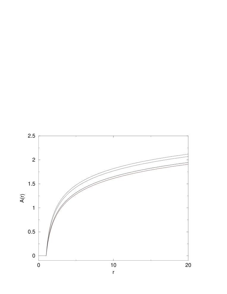
FIG. 1.: Solutions for $A(r)$ (in $\epsilon=1$ units with $A(\epsilon)$ set to zero) for various values of $a\equiv\kappa{\widetilde{L}}$, $b\equiv(\kappa-2){\widetilde{L}}$ (and $\xi$ - see below). From top to bottom: $\xi=1$, $a=2$, $b=-1$; $\xi=1$, $a=1$, $b=-1$; $\xi=1$, $a=2$, $b=-1.2$; $\xi=1$, $a=1$, $b=-1.2$ (The $\xi=2$ counterparts of the lines for $B(r)$ in Fig.2 coincide with the $\xi=1$ lines.) This plot shows that Solution A for the membrane is indeed diluting.

FIG. 2.: Solutions for $B(r)$ (in $\epsilon=1$ units) for various values of $a\equiv\kappa{\widetilde{L}}$, $b\equiv(\kappa-2){\widetilde{L}}$ and $\xi$. From top to bottom: $\xi=2$, $a=1$, $b=-1$; $\xi=2$, $a=1$, $b=-1.2$; $\xi=1$, $a=2$, $b=-1$; $\xi=1$, $a=1$, $b=-1$; $\xi=1$, $a=2$, $b=-1.2$; $\xi=1$, $a=1$, $b=-1.2$. This plot shows that Solution A for the membrane is indeed diluting.

FIG. 3.: Solutions for $A(r)$ (in $\epsilon=1$ units with $A(\epsilon)$ set to zero) for ${\widetilde{\Lambda}}=1$ (see below) and various values of $a\equiv{\widetilde{L}}/\xi$. From top to bottom: $a=10^{8}$, $a=10^{6}$, $a=10^{4}$ and $a=1$. (The ${\widetilde{\Lambda}}\not=1$ counterparts of the solid lines for $B(r)$ in Fig.4 cannot be distinguished from the $a={\widetilde{\Lambda}}=1$ line.) This plot shows that the $\xi>0$ branch of the $\eta=-1$ 3-brane solution is indeed diluting.

FIG. 4.: Solutions for $B(r)$ (in $\epsilon=1$ units) for various values of ${\widetilde{\Lambda}}$ and $a\equiv{\widetilde{L}}/\xi$. From top to bottom: $a=1$ with ${\widetilde{\Lambda}}=.1$, ${\widetilde{\Lambda}}=1$, ${\widetilde{\Lambda}}=10$, ${\widetilde{\Lambda}}=100$ (solid lines) ; and ${\widetilde{\Lambda}}=1$ with $a=10^{-6}$, $a=10^{4}$, $a=10^{8}$ (dashed lines) ; This plot shows that the $\xi>0$ branch of the $\eta=-1$ 3-brane solution is indeed diluting.

FIG. 5.: The solid lines are zeros of $4VU(V+U)+4V+z(U-V-1)$ while the dot-dashed lines are the zeros of $-2z(2V+U-1)+8V^{2}U$. In the region in between dashed lines there are no real solutions of (167).

FIG. 6.: The solid line represents the zeros of $4VU(V+U)+4V+z(U-V-1)$; inside the dashed pockets there are no real solutions of (167).

FIG. 7.: The solid lines are zeros of $12V^{3}+z(U-V-1)-12V(U^{2}-1)$ that approach the following curves for $\left|z\right|\gg 1$: $I-II$ boundary: $V=-2/3$, $III-IV$ boundary: $z=12V^{2}$ and $I-VI$ boundary: $z=-27.3V^{2}$. The dot-dashed line between $II$ and $III$ is $z=72V^{2}$ while the one between $IV$ and $V$ that approaches $z=9.6V^{2}$ for $z\gg 1$ consists of zeros of $\kappa$. Inside the dashed pockets there are no real solutions of (204).

FIG. 8.: The solid lines are the zeros of $12V^{3}+z(U-V-1)-12V(U^{2}-1)$ that approach the following curves for $\left|z\right|\gg 1$: $II-III$ boundary: $z=12.7V^{2}$, $V-VIII$ boundary: $z=-3.66V^{2}$ and $I-VIII$ boundary: V=-2/3. The dot-dashed line between $III$ and $IV$ is $z=72V^{2}$ while the one between $I$ and $II$ representing the zeros of $\kappa$ approaches $z=-3.66V^{2}$ for $V\gg 1$ (the third dot-dashed line consists also of zeros of $\kappa$). Inside the dashed pockets there are no real solutions of (204).

REFERENCES

- [1] G. Dvali and G. Gabadadze, Phys. Rev. D63 (2001) 065007.
- [2] O. Corradini, A. Iglesias, Z. Kakushadze and P. Langfelder, Phys. Lett. B521 (2001) 96.
- [3] Z. Kakushadze, JHEP 0110 (2001) 031.
- [4] G. Dvali, G. Gabadadze, X.-r. Hou and E. Sefusatti, hep-th/0111266.
- [5] R. Gregory, Nucl. Phys. B467 (1996) 159.
- [6] G. Dvali, G. Gabadadze and M. Porrati, Phys. Lett. B485 (2000) 208.
- [7] O. Corradini, A. Iglesias, Z. Kakushadze and P. Langfelder, Mod. Phys. Lett. A17 (2002) 795.
- [8] G. Dvali, G. Gabadadze and M. Shifman, hep-th/0202174.
- [9] N. Arkani-Hamed, S. Dimopoulos and G. Dvali, Phys. Lett. B429 (1998) 263.
- [10] E. Witten, hep-ph/0002297.