The static effective action for non-commutative QED at high temperature

Abstract

In this paper, we systematically study the effective action for non-commutative QED in the static limit at high temperature. When $\theta p^{2}\ll 1$, where $\theta$ represents the magnitude of the parameter for non-commutativity and $p$ denotes a typical external three momentum, we show that this leads naturally to a derivative expansion in this model. The study of the self-energy, in this limit, leads to nontrivial $\theta$ dependent corrections to the electric and magnetic masses, which exist only above a certain critical temperature. The three point and the four point amplitudes are also studied as well as their relations to the Ward identities in this limit. We determine the closed form expression for the current involving only the spatial components of the gauge field and present the corresponding static effective action, which is gauge invariant.

I Introduction

Thermal field theories kapusta:book89lebellac:book96das:book97 are of interest for a variety of reasons. As is well known by now, thermal amplitudes and, therefore, the effective actions have a non-analytic structure weldon . Consequently, they are best studied in some limit. The static limit, where the external energies are set equal to zero, is one such limit and is of interest in the study of a plasma at very high temperatures because several physical quantities such as the screening and the magnetic masses are defined in this limit. It is also known that because of infrared divergences in a thermal field theory, one needs to perform a resummation to obtain meaningful gauge independent quantities at high temperature. While, in principle, the resummation can involve general self-energy and vertex corrections (as internal insertions), the dominant contributions to the screening and magnetic masses come from the static limit of these corrections (namely, the zero modes contribute the most). It is for these reasons that the study of the static limit of the effective action at high temperature is quite useful. The hard thermal loops and the static effective actions in conventional gauge theories have been well studied in the literature Braaten:1990it ; frenkel:1991ts .

In this paper, we intend to carry out a corresponding analysis for non-commutative QED. Non-commutative theories Seiberg:1999vs ; Fischler:2000fv ; hayakawa ; Arcioni:1999hw ; Landsteiner:2000bw ; Szabo:2001kg ; Douglas:2001ba ; Chu:2001fe ; VanRaamsdonk:2001jd ; Bonora:2000ga ; Brandt:2002rw are defined on a manifold where coordinates do not commute, rather they satisfy

$$\left[x^{\mu},x^{\nu}\right]=i\theta^{\mu\nu}$$ (1)

where $\theta^{\mu\nu}$ is an anti-symmetric constant tensor. For unitarity to hold in these theories gomis , conventionally, one assumes that $\theta^{0i}=0$, namely, we will assume that only the spatial coordinates do not commute while the time coordinate commutes with space coordinates. Furthermore, we note that the experimental bound on the magnitude of the parameter of non-commutativity leads to sean

$$\theta=|\theta^{ij}|\leq(10\,{\rm TeV})^{-2}\approx 10^{-34}\,{\rm cm}^{2}$$ (2)

The parameter for non-commutativity is, therefore, expected to be very small.

The non-commutativity of the coordinates leads to a modified product on such a manifold, the Gröenwald-Moyal star product, namely

$$f(x)\star g(x)=e^{\frac{i}{2}\theta^{\mu\nu}\partial^{(\eta)}_{\mu}\partial^{(\xi)}_{\nu}}\,\left.f(x+\eta)g(x+\xi)\right|_{\eta=\xi=0}$$ (3)

As a consequence of the nontrivial nature of the star product (namely, star products do not commute), the Maxwell theory acquires a non-Abelian structure, namely, the action for the Maxwell action on a non-commutative manifold takes the form

$$S=\int d^{4}x\,\left(-\frac{1}{4}\,F_{\mu\nu}\star F^{\mu\nu}\right)$$ (4)

where the field strength tensor has the form

$$F_{\mu\nu}=\partial_{\mu}A_{\nu}-\partial_{\nu}A_{\mu}-ie\left[A_{\mu},A_{\nu}\right]_{\rm MB}=\partial_{\mu}A_{\nu}-\partial_{\nu}A_{\mu}-ie\left(A_{\mu}\star A_{\nu}-A_{\nu}\star A_{\mu}\right)$$ (5)

The action (4) is invariant under a gauge transformation

$$A_{\mu}\rightarrow U\star A_{\mu}\star U^{-1}-\frac{i}{e}\,U\star\partial_{\mu}U^{-1}$$ (6)

which is reminiscent of non-Abelian gauge transformations in conventional theories. The structure of the field strength tensor in (5) also makes it clear that Maxwell’s theory on a non-commutative manifold involves self-interactions. Consequently, since the action in (4) is an interacting theory, we neglect the fermions, although we can add fermions in a natural manner. There is a second reason for neglecting the fermions. It is known that fermion loops only lead to planar contributions which are the same as in conventional QED and we are interested in $\theta$ dependent corrections to various physical quantities.

The paper is organized as follows. In section II, we describe in detail the tensor structure for the self-energy in non-commutative QED at finite temperature. We also give the perturbative result for the self-energy in the static limit. This can be exactly evaluated in a closed form, as was observed earlier Brandt:2002aa . Here, we clarify the reason for such a simplification. We determine the $\theta$ dependent screening and the magnetic masses in this theory at the one loop level and show that these contributions are nontrivial only for temperatures above a certain temperature. In section III, we study the leading terms in the three point and the four point amplitudes in some detail and show that their structure is consistent with what we will expect from the Ward identities. In fact, the three point function can be completely expressed in terms of the static self-energy. This is a consequence of the fact that amplitudes with an odd number of temporal indices (such as $\Gamma_{000}$) vanish. On the other hand, not all nontrivial components of the four point function can be expressed in terms of the lower order amplitudes, since, in this case, $\Gamma_{0000}$ neither vanishes nor is constrained by the Ward identity and, consequently, needs to be evaluated independently. In section IV, we solve the Ward identity and determine, in terms of the self-energy, a simple expression for the current which depends on the spatial components of the gauge field. In section V, we present a closed form effective action for the static amplitudes, with spatial tensor structures, which is valid at high temperatures in the region $\theta p^{2}\ll 1$. This gauge invariant action (see Eq. (72)) is expressed in terms of functions which may be related to open Wilson lines.

II Self-energy for non-commutative QED in the static limit at high temperature

In this section, we will discuss the tensor decomposition of the self-energy in non-commutative QED at finite temperature. Using this, we will evaluate the self-energy in the static limit at high temperature and study various masses that follow.

Let us begin by recalling that in a conventional theory, at zero temperature, there are two natural tensor structures, $\eta^{\mu\nu}$ and $p^{\mu}$, the external momentum, with which we can describe the self-energy. In a non-commutative theory at finite temperature, we have additional structures such as $\theta^{\mu\nu}$ and $u^{\mu}$, the velocity of the heat bath. To determine the most general, second rank symmetric tensor constructed from $\eta^{\mu\nu},p^{\mu},\theta^{\mu\nu},u^{\mu}$, let us proceed as follows. First, we note that there are seven distinct second rank symmetric tensor structures that we can form, namely, $\eta^{\mu\nu},u^{\mu}u^{\nu},p^{\mu}p^{\nu},\tilde{p}^{\mu}\tilde{p}^{\nu},(p^{\mu}u^{\nu}+p^{\nu}u^{\mu}),(p^{\mu}\tilde{p}^{\nu}+p^{\nu}\tilde{p}^{\mu}),(\tilde{p}^{\mu}u^{\nu}+\tilde{p}^{\nu}u^{\mu})$ where we have defined

$$\tilde{p}^{\mu}=\theta^{\mu\nu}p_{\nu}$$ (7)

By definition, $\tilde{p}^{\mu}$ is transverse to $p^{\mu}$ and, furthermore, it can also be easily verified that $u\cdot\tilde{p}=0$ since $\theta^{\mu\nu}$ only involves spatial indices. However, to leading order at high temperature, the Ward identities require that the self-energy be transverse to the external momentum. To obtain the most general second rank symmetric tensor that is also transverse, let us define

$$\hat{\eta}^{\mu\nu} = \eta^{\mu\nu}-u^{\mu}u^{\nu}$$

$$\hat{p}^{\mu} = p^{\mu}-(u\cdot p)u^{\mu}$$

$$\bar{u}^{\mu} = u^{\mu}-\frac{(u\cdot p)}{p^{2}}\,p^{\mu}$$ (8)

By construction, the “hat” variables are orthogonal to $u^{\mu}$ (the velocity is normalized to unity, $u\cdot u=1$) while $\bar{u}^{\mu}$ is orthogonal to $p^{\mu}$. It is easy to see now that we can construct four independent second rank symmetric tensors which are transverse so that the self-energy, for the photon, can be written in the form

$$\Pi^{\mu\nu}=A\,\left(\hat{\eta}^{\mu\nu}-\frac{\hat{p}^{\mu}\hat{p}^{\nu}}{\hat{p}^{2}}\right)+B\,\frac{p^{2}}{\hat{p}^{2}}\,\bar{u}^{\mu}\bar{u}^{\nu}+C\,\frac{\tilde{p}^{\mu}\tilde{p}^{\nu}}{\tilde{p}^{2}}+D\,(\bar{u}^{\mu}\tilde{p}^{\nu}+\bar{u}^{\nu}\tilde{p}^{\mu})$$ (9)

However, we note that the self-energy for the photon is even under charge conjugation ($\theta\rightarrow-\theta$) Sheikh-Jabbari:1999vm ; fernando , while the last structure in (9) is odd. Therefore, we must have $D=0$ and to all orders, the self energy can be parameterized as

$$\Pi^{\mu\nu}=A\,P^{\mu\nu}+B\,Q^{\mu\nu}+C\,R^{\mu\nu}$$ (10)

where we have defined

$$P^{\mu\nu}=\left(\hat{\eta}^{\mu\nu}-\frac{\hat{p}^{\mu}\hat{p}^{\nu}}{\hat{p}^{2}}\right),\quad Q^{\mu\nu}=\frac{p^{2}}{\hat{p}^{2}}\,\bar{u}^{\mu}\bar{u}^{\nu},\quad R^{\mu\nu}=\frac{\tilde{p}^{\mu}\tilde{p}^{\nu}}{\tilde{p}^{2}}$$ (11)

The tensors appearing in (11) are easily seen to be projection operators,

$$P^{\mu\lambda}P_{\lambda\nu}=P^{\mu}_{\nu},\quad Q^{\mu\lambda}Q_{\lambda\nu}=Q^{\mu}_{\nu},\quad R^{\mu\lambda}R_{\lambda\nu}=R^{\mu}_{\nu}$$ (12)

However, they are not orthonormal. In fact, it is easy to check that

$$P^{\mu\lambda}Q_{\lambda\nu}=0=Q^{\mu\lambda}R_{\lambda\nu},\quad P^{\mu\lambda}R_{\lambda\nu}=R^{\mu}_{\nu}$$ (13)

This suggests that a better basis to work with is given by $\overline{P}^{\mu\nu},Q^{\mu\nu},R^{\mu\nu}$ where

$$\overline{P}^{\mu\nu}=P^{\mu\nu}-R^{\mu\nu}$$ (14)

so that all the structures correspond to orthonormal projection operators. In this basis, we can parameterize the leading order self-energy at high temperature as

$$\Pi^{\mu\nu}=\overline{P}^{\mu\nu}\,\Pi_{\rm T}+Q^{\mu\nu}\,\Pi_{\rm L}+R^{\mu\nu}\,\tilde{\Pi}_{T}$$ (15)

The meaning of the various projections is quite clear. While $\overline{P}^{\mu\nu},Q^{\mu\nu},R^{\mu\nu}$ are all orthogonal to $p^{\mu}$, it is easy to see from their definitions in (11) and (14) that $\overline{P}^{\mu\nu}$ is, in addition, orthogonal to $u^{\mu}$ as well as to $\tilde{p}^{\mu}$. Similarly, $Q^{\mu\nu}$ is additionally transverse to $\tilde{p}^{\mu}$ and $R^{\mu\nu}$ to $u^{\mu}$. Thus, additionally, $\overline{P}^{\mu\nu}$ and $R^{\mu\nu}$ are transverse to $p^{i}$ (that is the reason for the subscript “T” in their form factors) while $Q^{\mu\nu}$ is not (which is why the subscript on the form factor is “L”). Furthermore, while $\overline{P}^{\mu\nu}$ and $R^{\mu\nu}$ are both orthogonal to $p^{i}$, the first is orthogonal to vectors in the non-commutative plane (if only two coordinates do not commute) while the second is not. Finally, let us note that

$$\overline{P}^{\mu\nu}+Q^{\mu\nu}+R^{\mu\nu}=\eta^{\mu\nu}-\frac{p^{\mu}p^{\nu}}{p^{2}}$$ (16)

With the parameterization of the self-energy in (15) in terms of orthonormal projection operators, several things simplify. First, we note that we can determine the various form factors as

$$\Pi_{\rm L}=\frac{p^{2}}{\hat{p}^{2}}\,u_{\mu}u_{\nu}\Pi^{\mu\nu},\quad\tilde{\Pi}_{\rm T}=\frac{\tilde{p}_{\mu}\tilde{p}_{\nu}}{\tilde{p}^{2}}\,\Pi^{\mu\nu},\quad(D-3)\Pi_{\rm T}=\eta_{\mu\nu}\Pi^{\mu\nu}-\Pi_{\rm L}-\tilde{\Pi}_{\rm T}$$ (17)

Here, $D$ represents the number of space-time dimensions. In particular, we note that when $D=3$, we do not have any information on the transverse form factor from these equations which has to be contrasted with the case in a conventional theory (for which the same happens if $D=2$). Adding in the tree level two point function, we can write to all orders

$$\Gamma^{\mu\nu}=\overline{P}^{\mu\nu}\,(p^{2}+\Pi_{\rm T})+Q^{\mu\nu}\,(p^{2}+\Pi_{\rm L})+R^{\mu\nu}\,(p^{2}+\tilde{\Pi}_{\rm T})+\frac{p_{\mu}p_{\nu}}{\xi}$$ (18)

where $\xi$ represents the gauge fixing parameter in a covariant gauge. Since the projection operators are orthonormal, the inverse can be easily obtained, leading to the propagator

$$D_{\mu\nu}=\overline{P}_{\mu\nu}\,\frac{1}{p^{2}+\Pi_{\rm T}}+Q_{\mu\nu}\,\frac{1}{p^{2}+\Pi_{\rm L}}+R_{\mu\nu}\,\frac{1}{p^{2}+\tilde{\Pi}_{\rm T}}+\xi\,\frac{p_{\mu}p_{\nu}}{p^{2}}$$ (19)

The poles in the propagator are distinct as a consequence of our choice of orthonormal projection operators (Had we used a different basis, the poles will be mixed and will need to be disentangled). We see that there are three physical poles (in addition to the unphysical one coming from the gauge fixing). The meaning of the three poles is easily understood as follows. First, we can define the screening mass, as in a conventional theory, as (our Minkowski metric has the signatures $(+,-,-,-)$)

$$m_{\rm el}^{2}=-\Pi_{\rm L}(p_{0}=0,p^{2}=-{\bf p}^{2}=m_{\rm el}^{2})$$ (20)

The conventional magnetic mass can also be defined as

$$m_{\rm mag}^{2}=-\Pi_{\rm T}(p_{0}=0,p^{2}=-{\bf p}^{2}=m_{\rm mag}^{2})$$ (21)

However, there is now a new transverse pole at

$$\tilde{m}_{\rm mag}^{2}=-\tilde{\Pi}_{\rm T}(p_{0}=0,p^{2}=-{\bf p}^{2}=\tilde{m}_{\rm mag}^{2})$$ (22)

This can be thought of as the screening length between magnetic fields in the non-commutative plane. This feature is new in non-commutative QED, since the non-commutative parameter can define a preferred direction in space.

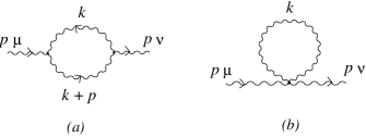
Figure 1: One-loop diagrams which contribute to the photon self-energy in non-commutative QED. The wavy lines represent photons and diagrams with ghost loops are understood to be included.

Let us now evaluate the self-energy, represented in figure 1, in the static limit at high temperature. We note that the calculation of the self-energy, in the static limit, was already done in Brandt:2002aa and the result was surprisingly very simple. Here, we would like to understand the reason for the simplicity of this result and then calculate the physical masses in the theory. To begin with, let us tabulate a few integrals gradshteyn that will be useful in the evaluation of the self-energy.

$$\int_{0}^{\infty}dx\,\frac{x}{e^{\frac{x}{T}}-1} = \frac{\pi^{2}T^{2}}{6}$$

$$\int_{0}^{\infty}dx\,\frac{\sin xy}{e^{\frac{x}{T}}-1} = \frac{\pi T}{2}\left(\coth\pi yT-\frac{1}{\pi yT}\right)$$

$$\int_{0}^{\infty}dx\,\frac{x\cos xy}{e^{\frac{x}{T}}-1} = \frac{1}{2y^{2}}-\frac{\pi^{2}T^{2}}{2}\,{\rm cosech}^{2}\pi yT$$ (23)

A direct application of the forward scattering amplitude method brandt:1993mj ; brandt:1993dkbrandt:1997se leads, in the hard thermal loop approximation, to the the self-energy of the form

$$\Pi^{\mu\nu}(p)=-\frac{4e^{2}}{(2\pi)^{3}}\int d^{3}k\,\frac{n_{B}(k)}{k}(1-\cos\tilde{p}\cdot k)\left.\left[\eta^{\mu\nu}-\frac{p^{\mu}k^{\nu}+p^{\nu}k^{\mu}}{p\cdot k}+\frac{p^{2}k^{\mu}k^{\nu}}{(p\cdot k)^{2}}\right]\right|_{k^{0}=k}$$ (24)

where $k=|{\bf k}|$ and $n_{B}$ represents the bosonic distribution function. Let us recall that the hard thermal loop approximation, in this theory, involves assuming

$$p\ll k\sim{\rm min}\,(T,\frac{1}{\tilde{p}})$$ (25)

Going to the rest frame of the heat bath and using (23), it now follows easily that

$$\eta_{\mu\nu}\Pi^{\mu\nu} = -\frac{8e^{2}}{(2\pi)^{3}}\int d^{3}k\,\frac{n_{B}(k)}{k}(1-\cos\tilde{p}\cdot k)$$ (26)

$$= -\frac{16e^{2}}{(2\pi)^{2}}\int_{0}^{\infty}\frac{dk\,k}{e^{\frac{k}{T}}-1}\,\left(1-\frac{\sin k|\tilde{p}|}{k|\tilde{p}|}\right)=-2e^{2}T^{2}\left[\frac{1}{3}-\frac{1}{\pi|\tilde{p}|T}\left(\coth\pi|\tilde{p}|T-\frac{1}{\pi|\tilde{p}|T}\right)\right]$$

where we have defined

$$|\tilde{p}|=|\theta^{ij}p_{j}|$$ (27)

While the calculation of the trace of the self-energy from (24) is simple, in the static limit, the calculations of $\Pi_{\rm L},\tilde{\Pi}_{\rm T}$ are not, and are manifestly non-local. However, with a little bit of algebra, which involves integration by parts of the relation

$$\frac{p^{\mu}k^{\nu}+p^{\nu}k^{\mu}}{p\cdot k}-\frac{p^{2}k^{\mu}k^{\nu}}{(p\cdot k)^{2}}=p_{\lambda}\frac{\partial}{\partial k_{\lambda}}\left(\frac{k^{\mu}k^{\nu}}{p\cdot k}\right)$$ (28)

it may be shown that Eq. (24) can be rewritten as

$$\Pi^{\mu\nu}=-\frac{4e^{2}}{(2\pi)^{3}}\int\frac{d^{3}k}{k}\,(1-\cos\tilde{p}\cdot k)\left.\left[\eta^{\mu\nu}n_{B}(k)+n^{\prime}_{B}(k)\,\frac{p^{0}k^{\mu}k^{\nu}}{p\cdot k}-(kn^{\prime}_{B}(k)-n_{B}(k))\frac{k^{\mu}k^{\nu}}{k^{2}}-n_{B}(k)\frac{\eta^{\mu 0}k^{\nu}+\eta^{\nu 0}k^{\mu}}{k}\right]\right|_{k^{0}=k}$$ (29)

where a prime denotes differentiation with respect to $k$. It is clear from (29) that the potentially non-local terms vanish in the static limit when $p^{0}=0$. Thus, we see that the self-energy is a local function in the static limit, with a simple form (obtained by using the symmetry of the ${\bf k}$ integral)

$$\Pi^{\mu\nu}_{\rm static}=\frac{4e^{2}}{(2\pi)^{3}}\int\frac{d^{3}k}{k}\,(1-\cos\tilde{p}\cdot k)\left.\left[-\eta^{\mu\nu}n_{B}(k)+(kn^{\prime}_{B}(k)-n_{B}(k))\frac{k^{\mu}k^{\nu}}{k^{2}}+n_{B}(k)\frac{2\eta^{\mu 0}\eta^{\nu 0}}{k}\right]\right|_{k^{0}=k}$$ (30)

There are several things to note from (30). First, the integrand, except for the trigonometric function (coming from the vertices of the non-commutative theory), is completely local and is independent of the external momentum. Since the trigonometric function does not involve $k^{0}$ (namely, $\theta^{0i}=0$), it can be taken outside the Matsubara sum in the imaginary time formalism and it is clear that the result, (30), can be obtained directly from the Matsubara sum of frequencies by setting the external momentum equal to zero (except in the trigonometric factor which is outside the sum and will give zero if the external momentum is naively set to zero). In this case, the sum is very simple and can be done in a trivial manner. In this sense, this result can be understood as the leading term in a derivative expansion. This is, in fact, supported by the structure of the theory. We know that amplitudes become non-analytic in a thermal field theory. However, once we are in the static limit, the amplitudes are analytic in $p^{i}$ (in the absence of infrared problems) so that a derivative expansion does make sense. We have shown earlier that although the amplitudes in a non-commutative theory are also non-analytic, the non-analyticity is not a consequence of any new branch cut. Therefore, we expect the general analytic behavior of the conventional thermal field theories to hold in a non-commutative theory at finite temperature. Furthermore, we note that because of the trigonometric function in (30), in the infrared limit $(1-\cos\tilde{p}\cdot k)\rightarrow 0$ and, consequently, infrared divergence is not a problem in such theories at finite temperature (namely, as $p^{i}\rightarrow 0$, the coupling vanishes in such theories). Therefore, in the static limit, we expect the amplitudes to be analytic in $p^{i}$, leading to the fact that a derivative expansion can be carried out. This also explains the simplicity of the form for the self-energy in the static limit. Namely, if we set all the external momentum to zero in the denominator (namely, the leading term in the derivative expansion), then, the integrand involves only one angular integral coming from the trigonometric function which is easy to carry out. We also note from the form of the amplitude in (30) that $\Pi^{0i}=\Pi^{i0}=0$ from the symmetry of the integrand. We will comment more on this in the next section.

The components of the self-energy, in the static limit, can now be easily calculated. Without going into the details, we simply note that, in the rest frame of the heat bath, the components of the self-energy take the forms

$$\Pi^{00}_{\rm static} = -\frac{2e^{2}T^{2}}{3}\left[1-\frac{3}{2}\left(\frac{\coth\pi|\tilde{p}|T}{\pi|\tilde{p}|T}-{\rm cosech}^{2}\pi|\tilde{p}|T\right)\right]$$

$$\Pi^{0i}_{\rm static} = 0$$

$$\Pi^{ij}_{\rm static} = -e^{2}T^{2}\left[\frac{\coth\pi|\tilde{p}|T}{\pi|\tilde{p}|T}+{\rm cosech}^{2}\pi|\tilde{p}|T-\frac{2}{(\pi|\tilde{p}|T)^{2}}\right]\frac{\tilde{p}^{i}\tilde{p}^{j}}{\tilde{p}^{2}}$$ (31)

Therefore, in this case, we have (see (17) in the rest frame of the heat bath)

$$\Pi_{\rm L}^{\rm static} = \Pi^{00}_{\rm static}=-\frac{2e^{2}T^{2}}{3}\left[1-\frac{3}{2}\left(\frac{\coth\pi|\tilde{p}|T}{\pi|\tilde{p}|T}-{\rm cosech}^{2}\pi|\tilde{p}|T\right)\right]$$

$$\tilde{\Pi}_{\rm T}^{\rm static} = \frac{\tilde{p}_{i}\tilde{p}_{j}}{\tilde{p}^{2}}\Pi^{ij}_{\rm static}=-e^{2}T^{2}\left[\frac{\coth\pi|\tilde{p}|T}{\pi|\tilde{p}|T}+{\rm cosech}^{2}\pi|\tilde{p}|T-\frac{2}{(\pi|\tilde{p}|T)^{2}}\right]$$

$$\Pi_{\rm T}^{\rm static} = \eta_{\mu\nu}\Pi^{\mu\nu}_{\rm static}-\Pi_{\rm L}^{\rm static}-\tilde{\Pi}_{\rm T}^{\rm static}=0$$ (32)

This shows that the conventional magnetic mass, $m_{\rm mag}$ defined in (21), vanishes as in QED on a commutative manifold. In the static limit, therefore, the self-energy (15) takes the form

$$\Pi^{\mu\nu}_{\rm static}=u^{\mu}u^{\nu}\,\Pi_{\rm L}^{\rm static}+\frac{\tilde{p}^{\mu}\tilde{p}^{\nu}}{\tilde{p}^{2}}\,\tilde{\Pi}_{\rm T}^{\rm static}$$ (33)

On the other hand, we see that both $\Pi_{\rm L}^{\rm static},\tilde{\Pi}_{\rm T}^{\rm static}$ have nontrivial contributions depending on $\theta$ (through $\tilde{p}$). This is to be expected since the effect of non-commutativity can be classically thought of as being equivalent to a background electromagnetic field. We note, in particular, that since $\tilde{\Pi}_{\rm T}^{\rm static}$ is nontrivial, there is a possibility, in this theory, to have a nontrivial magnetic mass in the non-commutative plane, even though the conventional magnetic mass vanishes. The screening mass and the “new” magnetic mass can be determined from the equations (see (20) and (22))

$$m_{\rm el}^{2} = -\Pi_{\rm L}^{\rm static}({\bf p}^{2}=-m_{\rm el}^{2})$$

$$\tilde{m}_{\rm mag}^{2} = -\tilde{\Pi}_{\rm T}^{\rm static}({\bf p}^{2}=-\tilde{m}_{\rm mag}^{2})$$ (34)

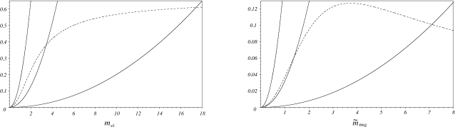
Figure 2: The electric and the magnetic masses in units of $(\pi\,\theta\,T)^{-1}$. The three solid lines are the plots of the parabola corresponding to the left hand side of Eqs. (34) for $(e\,\pi\,\theta\,T^{2})=2.5,\;5.6\;{\rm and}\;22.4$. The corresponding right hand sides are plotted using dashed lines.

These simultaneous equations can be solved graphically (see figure 2). We choose a coordinate system in which $\theta_{12}=-\theta_{21}=\theta$ represent the only non-vanishing components of $\theta_{ij}$. Then, setting $p^{3}=0$, we note that, in both the equations, the left and the right hand side give rise to parabola near the origin and, consequently, unless the slopes have appropriate values, there will be no intersection of the curves (and, therefore, no solution). This leads to the fact that, for a nontrivial screening mass to exist in this theory, we must have

$$T^{2}>T^{2}_{\rm c}=\frac{3\sqrt{5}}{2\pi e\theta}$$ (35)

Similarly, for a nontrivial “new” magnetic mass to exist, we must have

$$T^{2}>T_{\rm c}^{2}=\frac{3\sqrt{10}}{2\pi e\theta}$$ (36)

This is very interesting in that such a mass develops only above a critical temperature. Considering the smallness of $\theta$ (see (2)), we recognize that these temperatures are very high. Nonetheless, as a matter of principle, it is interesting to note that this behavior is quite similar to the propagation of waves in a wave guide or a plasma, which exists only above a critical cut-off frequency.

III Higher point amplitudes in the static limit at high temperature

In studying the higher point functions, in the static limit, at high temperature, we note that the complete symmetry of the amplitudes in the leading order approximation of the derivative expansion, leads to the result that any amplitude with an odd number of temporal indices vanishes. This is already evident in the results of the last section, namely, $\Pi^{0i}=0$. Therefore, we can concentrate only on amplitudes with an even number of temporal indices. In the case of the three point amplitude, this implies that we must have

$$\Gamma^{000}_{\rm static}=0=\Gamma^{0ij}_{\rm static}$$ (37)

and the only nontrivial components of the three point amplitude can be identified with $\Gamma^{00i},\Gamma^{ijk}$. Explicit calculations bear out this expectation.

From the discussion of the last section, we note that the leading contributions to any amplitude, in the static limit, can be obtained from the lowest order terms in a derivative expansion. Such a derivative expansion, as we have seen, corresponds to setting the external momenta equal to zero everywhere in the integrand except in the trigonometric functions. We note that the terms in the integrand, other than the trigonometric functions, have the general behavior that, in the hard thermal loop approximation, they are functions of zero degree in the external four momenta. Therefore, in the static limit, these factors become independent of the spatial momenta giving rise to the appearance of the leading contribution in a particular derivative expansion. The trigonometric functions, on the other hand, do not have this property. In the trigonometric functions, however, we can neglect contributions quadratic in the external momenta compared to terms linear in the external momenta. Thus, for example, in the three point amplitude diagram coming from three cubic vertices (see figure 3-a), the trigonometric functions coming from the vertices, can be simplified as

$$\sin\left(\frac{\tilde{p}_{1}\cdot k}{2}\right)\sin\left(\frac{\tilde{p}_{2}\cdot(k-p_{3})}{2}\right)\sin\left(\frac{\tilde{p}_{3}\cdot k}{2}\right)\approx\sin\left(\frac{\tilde{p}_{1}\cdot k}{2}\right)\sin\left(\frac{\tilde{p}_{2}\cdot k}{2}\right)\sin\left(\frac{\tilde{p}_{3}\cdot k}{2}\right)$$ (38)

Figure 3: Typical one-loop diagrams for the three point photon amplitude in non-commutative QED.

Expanding the second trigonometric function on the left hand side, it is easy to see that this corresponds to using the approximation that

$$\theta p^{2}\ll 1$$ (39)

where $p$ denotes the typical magnitude of the external momentum. Mathematically, such a derivative expansion would correspond to choosing

$$p\ll k,\qquad\theta pT\sim O(1)$$ (40)

which would automatically lead to (39).

Since the trigonometric functions do not involve any dependence on the energy ($\theta^{0i}=0$), in the regime (39), the calculation of any higher point amplitude, in the static limit, simplifies enormously and can be carried out directly in the imaginary time formalism. Explicit calculations show that, when all the graphs contributing to a given amplitude are summed, the trigonometric functions in the integrand of the $n$-point amplitude correspond to a product of $n$ factors of $\sin\left(\frac{\tilde{p}_{i}\cdot k}{2}\right)$ with $i=1,2,\cdots n$. This is consistent with the symmetry expected of the total amplitude, namely, since the only dependence on the external momenta is in the trigonometric functions in the leading order, and since the amplitude has to be symmetric under the exchange of external bosonic lines, the trigonometric functions must reflect this also. However, it is worth noting here that this is not expected to hold for individual graphs which is evident in the explicit calculations.

The recipe for calculating any higher point amplitude is now clear. For the $n$-point amplitude, for example, the integrand will involve $n$ trigonometric factors which can be taken outside the Matsubara sum, which has no dependence on the external momentum. Thus, for the three point amplitude, we obtain

$$\Gamma_{\mu\nu\lambda}^{\rm static}=ie^{3}T\int\frac{d^{3}k}{(2\pi)^{3}}\,\sin\left(\frac{\tilde{p}_{1}\cdot k}{2}\right)\sin\left(\frac{\tilde{p}_{2}\cdot k}{2}\right)\sin\left(\frac{\tilde{p}_{3}\cdot k}{2}\right)\sum_{n}\left[\frac{128k_{\mu}k_{\nu}k_{\lambda}}{((2\pi nT)^{2}+k^{2})^{3}}-\left(\frac{32\delta_{\mu\nu}k_{\lambda}}{((2\pi nT)^{2}+k^{2})^{2}}+{\rm cyclic}\right)\right]$$ (41)

Although (41) appears to involve three angles coming from the trigonometric functions (in which case the integration over spatial components would be nontrivial), we can use the identity

$$\sin\left(\frac{\tilde{p}_{1}\cdot k}{2}\right)\sin\left(\frac{\tilde{p}_{2}\cdot k}{2}\right)\sin\left(\frac{\tilde{p}_{3}\cdot k}{2}\right)=-\frac{1}{4}\left(\sin\tilde{p}_{1}\cdot k+\sin\tilde{p}_{2}\cdot k+\sin\tilde{p}_{3}\cdot k\right)$$ (42)

This is nice since each term involves only one angular integral which can be carried out using (23). Then, (41) becomes

$$\Gamma_{\mu\nu\lambda}^{\rm static}=-8ie^{3}T\int\frac{d^{3}k}{(2\pi)^{3}}\left(\sin\tilde{p}_{1}\cdot k+\sin\tilde{p}_{2}\cdot k+\sin\tilde{p}_{3}\cdot k\right)\sum_{n}\left[\frac{4k_{\mu}k_{\nu}k_{\lambda}}{((2\pi nT)^{2}+k^{2})^{3}}-\left(\frac{\delta_{\mu\nu}k_{\lambda}}{((2\pi nT)^{2}+k^{2})^{2}}+{\rm cyclic}\right)\right]$$ (43)

It is worth noting from this expression that when there is an odd number of temporal indices, the amplitude vanishes because of anti-symmetry in the Matsubara sum, which is consistent with the general structure of the static amplitudes in the leading order.

The actual evaluation of the thermal parts from the Matsubara sums can be carried out using the following relations

$$T\sum_{n}\frac{1}{(2\pi nT)^{2}+k^{2}} = \frac{n_{B}(k)}{k}+(T=0\,{\rm term})$$

$$T\sum_{n}\frac{1}{((2\pi nT)^{2}+k^{2})^{2}} = -\frac{1}{2k}\,\left(\frac{n_{B}(k)}{k}\right)^{\prime}+(T=0\,{\rm term})$$

$$T\sum_{n}\frac{1}{((2\pi nT)^{2}+k^{2})^{3}} = \frac{1}{4k}\left[\frac{1}{2k}\left(\frac{n_{B}(k)}{k}\right)^{\prime}\right]^{\prime}+(T=0\,{\rm term})$$ (44)

where prime denotes a derivative with respect to $k$. Using these as well as (23), the integrals can be evaluated and we find that the terms depending on Kronecker delta functions cancel out in the final result after carrying out the $d^{3}k$ integration. This may be seen by noticing that, when $\mu\nu\lambda$ are all spatial indices, we can write (43) in the form

$$\Gamma_{ijl}^{\rm static} = -2ie^{3}T\int\frac{d^{3}k}{(2\pi)^{3}}\,(\sin\tilde{p}_{1}\cdot k+\sin\tilde{p}_{2}\cdot k+\sin\tilde{p}_{3}\cdot k)\frac{\partial^{3}}{\partial k_{i}\partial k_{j}\partial k_{l}}\sum_{n}\log[(2\pi nT)^{2}+k^{2}]$$ (45)

$$= -2ie^{3}T\tilde{p}_{1,i}\tilde{p}_{1,j}\tilde{p}_{1,l}\int\frac{d^{3}k}{(2\pi)^{3}}\,\cos\tilde{p}_{1}\cdot k\sum_{n}\log[(2\pi nT)^{2}+k^{2}]+{\rm two\ similar\ terms}$$

which shows that only terms involving triple products of the same momentum are present in the final result for $\Gamma_{ijl}^{\rm static}$.

The nontrivial components of the three point amplitude, in the static limit, at leading order, then, take the forms

$$\Gamma_{00i}^{\rm static}(p_{1},p_{2},p_{3}) = ie\left[\tilde{p}_{1,\,i}\,\Pi_{00}^{\rm static}(p_{1})+{\rm cyclic}\right]$$

$$\Gamma_{ijk}^{\rm static}(p_{1},p_{2},p_{3}) = ie\left[\tilde{p}_{1,\,k}\,\Pi_{ij}^{\rm static}(p_{1})+{\rm cyclic}\right]$$ (46)

It now follows from (46) that

$$p_{3,\,i}\Gamma_{00i}^{\rm static}(p_{1},p_{2},p_{3}) = ie\left[p_{3}\cdot\tilde{p}_{1}\,\Pi_{00}^{\rm static}(p_{1})+p_{3}\cdot\tilde{p}_{2}\,\Pi_{00}^{\rm static}(p_{2})\right]$$

$$\approx -2ie\sin\left(\frac{\tilde{p}_{1}\cdot p_{2}}{2}\right)\left(\Pi_{00}^{\rm static}(p_{1})-\Pi_{00}^{\rm static}(p_{2})\right)$$

$$p_{3,\,k}\Gamma_{ijk}^{\rm static}(p_{1},p_{2},p_{3}) = ie\left[p_{3}\cdot\tilde{p}_{1}\,\Pi_{ij}^{\rm static}(p_{1})+p_{3}\cdot\tilde{p}_{2}\,\Pi_{ij}^{\rm static}(p_{2})\right]$$ (47)

$$\approx -2ie\sin\left(\frac{\tilde{p}_{1}\cdot p_{2}}{2}\right)\left[\Pi_{ij}^{\rm static}(p_{1})-\Pi_{ij}^{\rm static}(p_{2})\right]$$

where we have used the conservation of momentum in the intermediate steps as well as (39) to write

$$\tilde{p}_{1}\cdot p_{2}\approx 2\sin\left(\frac{\tilde{p}_{1}\cdot p_{2}}{2}\right)$$ (48)

This shows that the three point functions indeed satisfy simple Ward identities and that all the nontrivial components of the three point amplitude can, in fact, be determined from a knowledge of the self-energy.

Figure 4: Typical one-loop diagrams for the four point photon amplitude in non-commutative QED.

The general procedure outlined above can be used to evaluate the four point amplitude (see figure 4) in the leading order of the derivative expansion. In the static limit, this amplitude has the form

$$\Gamma_{\mu\nu\lambda\rho}^{\rm static}(p_{1},p_{2},p_{3},p_{4}) = 32e^{4}\int\frac{d^{3}k}{(2\pi)^{3}}\,\sin\left(\frac{\tilde{p}_{1}\cdot k}{2}\right)\sin\left(\frac{\tilde{p}_{2}\cdot k}{2}\right)\sin\left(\frac{\tilde{p}_{3}\cdot k}{2}\right)\sin\left(\frac{\tilde{p}_{4}\cdot k}{2}\right)$$ (49)

$$\!\!\times T\sum_{n}\left[\frac{24k_{\mu}k_{\nu}k_{\lambda}k_{\rho}}{((2\pi nT)^{2}+k^{2})^{4}}+\left(-\frac{4\delta_{\mu\nu}k_{\lambda}k_{\rho}}{((2\pi nT)^{2}+k^{2})^{3}}+\frac{\delta_{\mu\nu}\delta_{\lambda\rho}}{((2\pi nT)^{2}+k^{2})^{2}}+{\rm permutations}\!\right)\!\right]$$

As in the case of the three point function, this expression simplifies, in practice, upon using the trigonometric identity

$$8\sin\left(\frac{\tilde{p}_{1}\cdot k}{2}\right)\sin\left(\frac{\tilde{p}_{2}\cdot k}{2}\right)\sin\left(\frac{\tilde{p}_{3}\cdot k}{2}\right)\sin\left(\frac{\tilde{p}_{4}\cdot k}{2}\right) = C(p_{1},k)+C(p_{2},k)+C(p_{3},k)+C(p_{4})$$ (50)

$$-C(p_{1}+p_{4},k)-C(p_{2}+p_{4},k)-C(p_{3}+p_{4},k)$$

where we have defined

$$C(p,k)=1-\cos\tilde{p}\cdot k$$ (51)

For the spatial components, the integrand in (49) can be written in a similar form as in (45), so that no Kronecker delta functions appear in the final result when the $d^{3}k$ integration is carried out. Then, using (50), we obtain

$$\Gamma_{ijkl}^{\rm static}(p_{1},p_{2},p_{3},p_{4}) = e^{4}\left[f(\tilde{p}_{1})\tilde{p}_{1,i}\tilde{p}_{1,j}\tilde{p}_{1,k}\tilde{p}_{1,l}+f(\tilde{p}_{2})\tilde{p}_{2,i}\tilde{p}_{2,j}\tilde{p}_{2,k}\tilde{p}_{2,l}+\cdots\right.$$ (52)

$$-\left.f(\tilde{p}_{1}+\tilde{p}_{4})(\tilde{p}_{1}+\tilde{p}_{4})_{i}(\tilde{p}_{1}+\tilde{p}_{4})_{j}(\tilde{p}_{1}+\tilde{p}_{4})_{k}(\tilde{p}_{1}+\tilde{p}_{4})_{l}-\cdots\right]$$

where

$$f(\tilde{p})=\frac{\tilde{\Pi}_{\rm T}^{\rm static}(\tilde{p})}{e^{2}\,\tilde{p}^{2}}$$ (53)

and $\tilde{\Pi}_{\rm T}^{\rm static}$ is given in (32). Using (46), this can be written in terms of the three point amplitudes as

$$\Gamma_{ijkl}^{\rm static}(p_{1},p_{2},p_{3},p_{4}) = ie\left[\tilde{p}_{1,l}\Gamma_{ijk}^{\rm static}(p_{1}+p_{4},p_{2},p_{3})+\tilde{p}_{2,l}\Gamma_{ijk}^{\rm static}(p_{1},p_{2}+p_{4},p_{3})\right.$$ (54)

$$\quad\left.+\tilde{p}_{3,l}\Gamma_{ijk}^{\rm static}(p_{1},p_{2},p_{3}+p_{4})+\cdots\right]$$

where $\cdots$ represent terms needed to Bose symmetrize the amplitude. It is easy to see that this form is consistent with the static Ward identity

$$p_{4,l}\Gamma_{ijkl}^{\rm static}(p_{1},p_{2},p_{3},p_{4}) = ie\left[(\tilde{p}_{1}\cdot p_{4})\Gamma_{ijk}^{\rm static}(p_{1}+p_{4},p_{2},p_{3})+(\tilde{p}_{2}\cdot p_{4})\Gamma_{ijk}^{\rm static}(p_{1},p_{2}+p_{4},p_{3})\right.$$ (55)

$$\qquad\left.+(\tilde{p}_{3}\cdot p_{4})\Gamma_{ijk}^{\rm static}(p_{1},p_{2},p_{3}+p_{4})\right]$$

It is clear from these discussions of the static three and four point amplitudes that the components, where not all the indices are temporal, satisfy simple Ward identities, which follows from invariance under a static gauge transformation. Such components can, therefore, be recursively related. (The reason why such simple Ward identities hold in our case may be understood by noting that the contributions of the ghost particles, to this order, cancel out in the BRST identities.) The component of the four point amplitude with all temporal indices, $\Gamma_{0000}^{\rm static}$, on the other hand, is not constrained in the static limit and, therefore, cannot be related to lower order amplitudes. However, this component can be evaluated from (49) and it can be seen, after some algebra, that $\Gamma_{0000}^{\rm static}$ does not vanish. As a result, this can be taken as a new perturbative input in determining the complete static effective action. In fact, there will be a new perturbative input at every even order in perturbation, whenever the component of the amplitude with all temporal indices does not vanish.

IV The effective generating functional

The analysis of the previous section shows that all the nontrivial components of the three point function can be determined from a knowledge of the self-energy. However, at the level of the four point function, we also saw that we need to determine $\Gamma_{0000}$ independently since it is invariant under static gauge transformations. This component of the four point amplitude, on the other hand, would be essential in determining all the components of the five point amplitude. In fact, at every even order of the amplitudes, we expect new independent structures that cannot be determined from a knowledge of the lower order amplitudes. Therefore, it would be impossible to obtain a closed form expression for the complete effective action from a knowledge of the amplitudes to a given order. On the other hand, as we have seen, the components of the amplitudes with spatial indices only are related recursively, through Ward identities, to lower order amplitudes. Therefore, we can try to determine that part of the effective action which depends only on $A_{i}$.

Let $\Gamma[A_{i}]$ represent the part of the effective action at high temperature that depends only on the spatial components of the gauge field. Then, invariance under an infinitesimal static gauge transformation, leads to the Ward identity

$$\frac{\delta\Gamma[A_{k}]}{\delta\omega(x)}=\int dy\,\frac{\delta A_{i}(y)}{\delta\omega(x)}\frac{\delta\Gamma[A_{k}]}{\delta A_{i}(y)}=D_{i}\,\frac{\delta\Gamma[A_{k}]}{\delta A_{i}(x)}=0$$ (56)

where $\omega(x)$ represents the infinitesimal gauge transformation parameter depending only on the spatial coordinates. Equation (56) is simply a statement of the covariant conservation of current. Furthermore, under the approximation that we are using (see (39)), the covariant derivative, in the adjoint representation, takes the form

$$D_{i}=\partial_{i}+e(\partial_{j}A_{i})\,\tilde{\partial}_{j}$$ (57)

With this, the current conservation, (56), takes the form

$$\partial_{i}\,\frac{\delta\Gamma[A_{k}]}{\delta A_{i}}+e(\partial_{j}A_{i})\,\tilde{\partial}_{j}\,\frac{\delta\Gamma[A_{k}]}{\delta A_{i}} = 0$$

$${\rm or,}\quad\partial_{i}\left(\frac{\delta\Gamma[A_{k}]}{\delta A_{i}}+eA_{j}\tilde{\partial}_{i}\,\frac{\delta\Gamma[A_{k}]}{\delta A_{j}}\right) = 0$$ (58)

This determines that the quantity in the parenthesis vanishes up to a term that is transverse, namely,

$$\left(\delta_{ij}+eA_{j}\tilde{\partial}_{i}\right)\frac{\delta\Gamma[A_{k}]}{\delta A_{j}}=X_{i}^{\rm T}$$ (59)

such that

$$\partial_{i}X_{i}^{\rm T}=0$$ (60)

By taking the functional derivative of (59) with respect to $A_{j}$ and setting all the fields to zero, it can be easily determined that, to lowest order

$$X_{i}^{{\rm T}\,{\rm(lowest)}}=\Pi_{ij}^{\rm static}A_{j}$$ (61)

It is clear that $X_{i}^{\rm T}$ will contain higher order terms in the fields as well. However, it can be seen by taking higher order functional derivatives of (59) that the role of the higher order terms in $X_{i}^{\rm T}$ is to Bose symmetrize the higher point amplitude. Thus, keeping this Bose symmetrization in mind, we can neglect the contributions involving higher order terms in the fields in $X_{i}^{\rm T}$. In such a case, we can solve for the current from (59) and obtain

$$\frac{\delta\Gamma[A_{k}]}{\delta A_{i}}=\left(\delta_{ij}+eA_{j}\tilde{\partial}_{i}\right)^{-1}\,X_{j}^{{\rm T}\,{\rm(lowest)}}$$ (62)

The quantity in the parenthesis on the right hand side in (62) is an operator and hence does not have a unique left-right inverse. However, the one that is relevant, for the solution, is the right inverse which can be determined to be

$$\left(\delta_{ij}+eA_{j}\tilde{\partial}_{i}\right)^{-1}=\delta_{ij}-eA_{j}\tilde{\partial}_{i}+e^{2}A_{k}\tilde{\partial}_{i}A_{j}\tilde{\partial}_{k}-e^{3}A_{k}\tilde{\partial}_{i}A_{l}\tilde{\partial}_{k}A_{j}\tilde{\partial}_{l}+\cdots$$ (63)

Furthermore, we recognize from the definition of the covariant derivative (57) that

$$\partial_{j}\left(\delta_{ji}+eA_{i}\tilde{\partial}_{j}\right)=D_{i}$$ (64)

so that we can also write

$$\left(\delta_{ij}+eA_{j}\tilde{\partial}_{i}\right)^{-1}=D_{j}^{-1}\partial_{i}$$ (65)

Using (65), we can determine the current in (62) to be

$$j_{i}[A_{k}]=\frac{\delta\Gamma[A_{k}]}{\delta A_{i}}=D_{j}^{-1}\partial_{i}\Pi_{jk}^{\rm static}A_{k}$$ (66)

We note that this current manifestly satisfies covariant conservation since the self-energy is transverse. Furthermore, this closed form expression for the current can be explicitly checked to lead to the correct amplitudes, under Bose symmetrization.

The current is all we need for the generation of any amplitude. However, it will also be nice to determine the static effective action in a closed form. That involves functionally integrating the current which appears to be highly nontrivial. Nevertheless, we can obtain the effective action as explained in the next section.

V Discussion

Here we present a closed-form effective action for the static amplitudes (with spatial tensor indices) valid in the region (as in (39))

$$|p_{a}|\ll T,~{}~{}|p_{a}|\ll|{\theta}|^{-1/2},$$ (67)

where $a=1,2,\dots$ runs over the external momenta. In this region, we expect the internal momentum $k$ to be of the order given in (25).

Let us first define

$$C(p,A)=\int d^{4}x\exp[-ip\cdot x+ie{\tilde{p}}\cdot A(x)].$$ (68)

This is a function of an auxiliary 4-momentum $p$ and a functional of (the spatial components of) $A$. We will identify $p$ with the linear combinations of external momenta, as in (52). In the region (67), the general gauge-transformation (6) may be approximated as

$${\delta}A_{i}(x)=[{\partial}_{i}+ie({\tilde{\partial}}_{j}A_{i}(x)){\partial}_{j}]{\omega}(x).$$ (69)

$C$, defined in (68), is invariant under (69). To prove this, we note that

$${\delta}\left({\tilde{p}}\cdot A\right)=[{\tilde{p}}\cdot{\partial}+e({\tilde{\partial}}_{j}{\tilde{p}}\cdot A(x)){\partial}_{j}]{\omega}(x),$$

$${\delta}[\exp(ie{\tilde{p}}\cdot A(x)]=i\exp(ie{\tilde{p}}\cdot A)[{\tilde{p}}\cdot{\partial}+e({\tilde{\partial}}_{j}{\tilde{p}}\cdot A(x)){\partial}_{j}]{\omega}(x)$$

$$=i\exp(ie{\tilde{p}}\cdot A){\tilde{p}}\cdot{\partial}{\omega}-{\tilde{\partial}}_{j}[\exp(ie{\tilde{p}}\cdot A){\partial}_{j}{\omega}],$$ (70)

where we have used $\tilde{\partial}\cdot\partial=0$. Substituting (70) into (68) and integrating by parts (so that ${\tilde{\partial}}_{j}$ differentiates the $e^{-ip\cdot x}$) we obtain

$${\delta}C=i\int d^{4}xe^{-ip\cdot x}\exp(ie{\tilde{p}}\cdot A)[{\tilde{p}}\cdot{\partial}{\omega}-{\tilde{p}}\cdot{\partial}{\omega}]=0.$$ (71)

Now we can construct the effective action in terms of $C$:

$$\Gamma={1\over 2\times(2\pi)^{8}}\int d^{4}pf({\tilde{p}})C(p,A)C(-p,A)={1\over 2\times(2\pi)^{8}}\int d^{4}pf({\tilde{p}})|C(p,A)|^{2},$$ (72)

where $f$ is defined by (53).

That $\Gamma$ in (72) is the correct effective action follows because it trivially agrees with (31) and (32) to order $e^{2}$, it is gauge-invariant, and it gives the functional dependence on the ${\tilde{p}}_{a}$ ($a=1,2,3,\dots\nu$ for the $\nu$-point function) typified by (52). We have verified explicitly that $\Gamma$ gives the 3- and 4-point functions correctly.

It is much more difficult to find an effective action, not assuming both inequalities in (67), but just

$$|p_{a}|\ll T.$$ (73)

In this case we must use the exact gauge transformation (6), not just the approximate one in (69). But we note that $C$ in (68) does have a generalization which is gauge-invariant under the exact gauge-transformation (6). This generalization is

$$W(p,A)=\int{\rm d}^{4}x\exp{(-ip\cdot x)}\star P\exp{\left[ie\int_{0}^{1}{\rm d}\xi\,\tilde{p}\cdot A(x+\xi\tilde{p})\right]},$$ (74)

where $P$ denotes path ordering on the manifold characterized by the star product (3). $W(p,A)$ represents the Fourier transform of a gauge invariant open Wilson line, extending along a straight path from $x$ to $x+\tilde{p}$ VanRaamsdonk:2001jd ; Armoni:2001uw . Note that, if (67) is assumed, $W$ reduces just to $C$.

However, the thermal effective action (when (67) is not assumed) is not obtained just by replacing $C$ by $W$ in (72). The reason is that the internal photon momentum $k$ is expected to be of order $1/(|\theta||p_{a}|)$ and therefore (without (67)) we cannot make the hard thermal loop approximation of neglecting $|p_{a}|$ compared to $|k|$. The amplitudes are then much more complicated, and we cannot expect them to be expressible in terms of a single function $f$ as in (72).

Acknowledgment:

We would like to thank the referee for helpful comments. This work was supported in part by US DOE Grant number DE-FG 02-91ER40685, by CNPq and FAPESP, Brasil.

References

• (1) J. I. Kapusta, Finite Temperature Field Theory (Cambridge University Press, Cambridge, England, 1989);
M. L. Bellac, Thermal Field Theory (Cambridge University Press, Cambridge, England, 1996);
A. Das, Finite Temperature Field Theory (World Scientific, NY, 1997).
• (2) H. A. Weldon, Phys. Rev. D47, 594 (1993), P. F. Bedaque and A. Das, Phys. Rev. D47, 601 (1993), A. Das and M. Hott, Phys. Rev. D53, 2252 (1996).
• (3) E. Braaten and R. D. Pisarski, Nucl. Phys. B337, 569 (1990); Nucl. Phys. B339, 310 (1990).
• (4) J. Frenkel and J. C. Taylor, Nucl. Phys. B334, 199 (1990) ;Nucl. Phys. B374, 156 (1992).
• (5) N. Seiberg and E. Witten, JHEP 09, 032 (1999).
• (6) W. Fischler, J. Gomis, E. Gorbatov, A. Kashani-Poor, S. Paban, and P. Pouliot, JHEP 05, 024 (2000); W. Fischler, E. Gorbatov, A. Kashani-Poor, R. McNees, S. Paban, P. Pouliot, JHEP 06, 032 (2000).
• (7) M. Hayakawa, Phys. Lett. B478, 394 (2000).
• (8) G. Arcioni and M. A. Vazquez-Mozo, JHEP 01, 028 (2000).
• (9) K. Landsteiner, E. Lopez, and M. H. G. Tytgat, JHEP 09, 027 (2000); JHEP 06, 055 (2001).
• (10) R. J. Szabo, hep-th/0109162 (2001)
• (11) M. R. Douglas and N. A. Nekrasov, Rev. Mod. Phys. 73, 977 (2002).
• (12) A. Armoni, R. Minasian and S. Theisen, Phys. Lett. B 513, 406 (2001); C.-S. Chu, V. V. Khoze, and G. Travaglini, Phys. Lett. B513, 200 (2001); C.-S. Chu, V. V. Khoze, and G. Travaglini, hep-th/0112139 (2001).
• (13) M. Van Raamsdonk, JHEP 11, 006 (2001).
• (14) A. Armoni and E. Lopez, Nucl. Phys. B 632, 240 (2002).
• (15) A. Armoni, Nucl. Phys. B 593, 229 (2001); L. Bonora and M. Salizzoni, Phys. Lett. B504, 80 (2001).
• (16) F. T. Brandt, A. Das, J. Frenkel, D. G. C. McKeon and J. C. Taylor, Phys. Rev. D66, 045011 (2002).
• (17) See, for example, J. Gomis and T. Mehen, Nuc. Phys. B591, 265 (2000), O. Aharony, J. Gomis and T. Mehen, JHEP 09, 023 (2000).
• (18) M. Chaichian, M. M. Sheikh-Jabbari and A. Tureanu, Phys. Rev. Lett. 86, 2716 (2001); S. M. Carroll, J. A. Harvey, V. A. Kostelecky, C. D. Lane and T. Okamoto, Phys. Rev. Lett. 87, 141601 (2001).
• (19) F. T. Brandt, J. Frenkel and D. G. C. McKeon, Phys. Rev. D 65, 125029 (2002).
• (20) M. M. Sheikh-Jabbari, Phys. Rev. Lett. 84, 5265 (2000).
• (21) F. T. Brandt, A. Das and J. Frenkel, Phys. Rev. D65, 085017 (2002).
• (22) I. S. Gradshteyn and M. Ryzhik, “Table of Integrals, Series and Products” (Academic, New York, 1980).
• (23) F. T. Brandt, J. Frenkel, J. C. Taylor, and S. M. H. Wong, Can. J. Phys. 71, 219 (1993).
• (24) F. T. Brandt and J. Frenkel, Phys. Rev. D47, 4688 (1993); Phys. Rev. D56, 2453 (1997).