Imperial/TP/01-02/25

IHES/P/02/57

hep-th/0212081

December, 2002

Large Gauge Transformations in M-theory

J. Kalkkinen^ab and K.S. Stelle^a

^a The Blackett Laboratory, Imperial College

Prince Consort Road, London SW7 2BZ, U.K.

and

^b Institut des Hautes Études Scientifiques, Le Bois-Marie

35, Route de Chartres, Bures-sur-Yvette F-91440, France

Dedicated to the memory of Sonia Stanciu

We cast M-brane interactions including intersecting membranes and five-branes in manifestly gauge invariant form using an arrangement of higher dimensional Dirac surfaces. We show that the noncommutative gauge symmetry present in the doubled M-theory formalism involving dual 3-form and 6-form gauge fields is preserved in a form quantised over the integers. The proper context for discussing large noncommutative gauge transformations is relative cohomology, in which the 3-form transformation parameters become exact when restricted to the five-brane worldvolume. We show how this structure yields the lattice of M-theory charges and gives rise to the conjectured 7D Hopf–Wess–Zumino term.

Email: jussi.kalkkinen@ihes.fr, k.stelle@ic.ac.uk

1 Introduction

The classification of stable states in string and M-theory is important not only for establishing the spectrum of the theory, but also for understanding the physical equivalences of apparently different configurations. In string theory, where we know how branes interact through virtual open strings, the dynamics is well in control, at least in the Ramond–Ramond sector [1, 2]. In M-theory, this understanding is still largely missing for want of concrete control of the higher unstable modes, as well as of models for coinciding branes. Some aspects of the full interacting theory have been discussed in terms of Matrix-theory, of holography and of anomaly considerations. For instance, we know that the number of degrees of freedom in a system of coinciding five-branes grows cubically as a function of the number of branes [3, 4].

The M-theory spectrum contains, among other objects, membranes and their magnetic duals, five-branes. In addition to these, there are wave-like solutions and gravitational instantons that bear similarities to particles and six-branes, while boundaries of the 11D space can be interpreted as nine-branes [5, 6]. Though these excitations also reduce to D-branes in weakly coupled string theory, they are inherently gravitational in nature. The worldvolumes of such solitons also support solitons themselves: membranes may end on five-brane worldvolumes, with the ends being described by worldvolume self-dual strings [7, 8]. There are many more examples.

The aim of this article is to find ways to describe this multitude of branes and their intersections simply in terms of geometry. It appears that five-branes play a special rôle in this and that the geometrical description makes use of the relative cohomology of the spacetime and five-brane worldvolume. The elements of this cohomology come very close to being the physically significant equivalence classes of brane configurations. Related work on D2-branes in WZW has appeared in [9]. Other attempts in M-theory have been discussed e.g. in Refs [10, 11].

A more refined tool for analysing the geometry of M-branes is provided by the gauge symmetry algebra that combines bulk global (large) gauge transformations in bound M2–M5-brane systems with bulk diffeomorphisms. This system is subject to chiral anomalies on the five-brane worldvolume, requiring an extensive anomaly-cancelling mechanism. The purely gauge subalgebra of this relates to a “doubled” formalism [12] of 11D supergravity including both a 3-form $C$ and a 6-form $\tilde{C}$ gauge field; the essential commutator here is $[\delta_{3},\delta_{3}^{\prime}]=\delta_{6}$, where $\delta C=\Lambda_{{\scriptscriptstyle 3}}$, $\delta\tilde{C}=\Lambda_{{\scriptscriptstyle 6}}+{\textstyle{\frac{{\scriptstyle 1}}{\scriptstyle 2}}}\Lambda_{{\scriptscriptstyle 3}}\wedge C$ and for $\delta_{6}$ in the commutator one has $\Lambda_{{\scriptscriptstyle 6}}=\Lambda_{{\scriptscriptstyle 3}}^{\prime}\wedge\Lambda_{{\scriptscriptstyle 3}}$. The 3-form and 6-form parameters of these transformations must be closed but need not be exact, permitting thus also “large” gauge transformations, depending on the cohomology of the underlying spacetime. In this article, we shall refer to this algebra as the “M-theory gauge algebra.” For earlier work on the doubled formalism cf. e.g. Ref. [13].

We shall show how the M-theory gauge algebra survives in the global formulation of the theory, including the large gauge transformations, provided that one refines the notion of cohomological nontriviality to that of nontriviality in relative cohomology: $\Lambda_{3}$ must reduce to an exact form when restricted to five-brane worldvolumes.

There are several special features of M-theory five-branes that we shall have to contend with. The first observation is that, although the static five-brane solutions are non-singular, fluctuations around them become singular owing to concentration of waves at the horizon. Accordingly, one needs to introduce a $d=6$ worldvolume action for the five-brane [14, 15, 16, 17], (cf. also [18]); this acts as a source for the external 11D gauge fields and gravity [19]. The introduction of such a delta-function source will require careful regularisation at the brane surface, however.

Another distinctive feature is the way in which the cancellation of anomalies under chiral transformations of worldvolume determinants takes place. Though the bulk theory is known to contain $CR^{4}$-terms that give rise under diffeomorphisms to anomaly inflow onto the five-brane worldvolume, this is not quite sufficient to cancel all of the chiral anomalies, since an anomalous term proportional to the second Pontryagin class of the normal bundle remains [14]. Cancelling this part of the anomaly seems to involve understanding the details of the geometry of the $C$-field [20]. This would require a detailed description of the behaviour of the $C$-field solution under diffeomorphisms, which we do not include in this article.

The plan of the paper is as follows: we describe the dynamics of interacting M-branes perturbatively in Section 2. In Section 3 we formulate the model in such a way that invariance under large gauge symmetries becomes manifest. The independence of this description from the various choices of Dirac surfaces that we have to make is shown in Section 4. This provides a new derivation for the known relationships between the brane tensions. Finally, Section 5 contains a short description of the gauge and diffeomorphism algebras. We have tried to make the paper self-contained both physically and mathematically; many of the mathematical tools that we use are explained in the appendices.

2 Perturbative supergravity

The bosonic part of the 11D supergravity action [19] involves the metric and a 3-form $C$. The form-field part can be written as

$$S_{\mathrm{form}} = ~{}\frac{1}{\kappa}\int_{X}\frac{1}{2\eta}~{}G\wedge*G-\frac{1}{6}~{}C\wedge G\wedge G~{},$$ (1)

where $G\equiv{\mathrm{d}}C$ is the field-strength and $X$ is the 11D spacetime. We will later consider gravitational corrections to this action. The 3-form field can be naturally coupled to membranes while its electromagnetic dual 6-form $\tilde{C}$, to be more properly defined later, couples to five-branes. The five-brane supports a $d=6$ chiral $N=2$ tensor theory on its worldvolume. This theory involves an antisymmetric rank-two tensor $b$, with (anti-)self-dual field strength $h$, and five real scalars. This means that we should couple the bulk action to sources of the form

$$S_{\mathrm{CS}} = \int_{W_{6}}\frac{\alpha}{2}h\wedge*h+\beta~{}\iota^{*}\tilde{C}+\gamma~{}h\wedge\iota^{*}C$$ (2)

$$\qquad+\rho\int_{W_{2}}b+\tau\int_{W_{3}}C~{}.$$

We will fix the coefficients in units of the Newton constant $\kappa$ presently, by requiring gauge invariance. Gauge invariance will also impose geometrical constraints on the currents, cf. App. A.1, which appear here as volume forms for integration domains.

Figure 1: Some M-theory solitons.

Apart from the fermions, we will not pay particular attention here to a number of other worldvolume interactions. For instance the kinetic terms for bulk gravity and the worldvolume scalars follow from

$$S_{\mathrm{kinetic}} = \frac{1}{\kappa\eta^{3}}\int_{X}{\cal R}*1+T_{6}\int_{W_{6}}{\mathrm{d}}^{6}\sigma^{i}\sqrt{|\det G_{ij}|}$$ (3)

$$+T_{3}\int_{W_{3}}{\mathrm{d}}^{3}\sigma^{\mu}\sqrt{|\det G_{\mu\nu}|}~{},$$

where $G_{ij},G_{\mu\nu}$ are suitable pull-backs [14, 15, 16, 17] of the bulk metric and $T_{3}$,$T_{6}$ are brane tensions. There are many more. Neither will we include explicit dependence on worldvolume scalars, as these, as well as other twisting data such as the covariant derivative on the five-brane normal bundle, are implicit in the inclusions $\iota$ at the classical level. Furthermore, Wess–Zumino terms built out of these scalars and covariant derivatives would transform under transverse diffeomorphisms only, and are therefore not directly related to the gauge symmetries considered here; they play a rôle in anomaly cancellation, however.

What singles out the retained terms in $S_{\mathrm{form}}+S_{\mathrm{CS}}$, though, is the fact that these are the only gauge non-invariant Chern–Simons type terms that we can write down, i.e. terms of the form ${\mathrm{d}}^{-1}\omega$, where $\omega$ is some closed form. This means that these are the only terms that will transform nontrivially under gauge transformations, while all others remain inert by definition.

In addition to these worldvolume terms it turns out to be necessary to consider further Wess–Zumino type contributions. These terms have no apparent raison d’être from the point of view of the physical 11D spectrum, but will turn out to be crucial in defining a manifestly gauge invariant action using Dirac surfaces:

$$S_{\mathrm{WZ}} = \zeta\int_{W_{7}}C\wedge G+\frac{\xi}{2}\int_{W_{8}}G\wedge G~{}.$$ (4)

In particular, these terms will prove to be essential for obtaining the correct charge lattice. Here, too, we leave the integration domains as well as the coefficients as yet undetermined, which will allow us to retain the option of setting them to zero later if necessary. The total action is then the sum

$$S=S_{\mathrm{kinetic}}+S_{\mathrm{form}}+S_{\mathrm{CS}}+S_{\mathrm{WZ}}\equiv S_{\mathrm{kinetic}}+S_{\mathrm{gauge}}\ .$$ (5)

We will restrict our attention to the part of this relevant to gauge symmetry, $S_{\mathrm{gauge}}$. The constraints on brane tensions will guarantee that the Wess–Zumino part is proportional to $\hbar$, and thus can be thought of as a quantum mechanical effect. It will turn out that the Wess–Zumino terms do not live in eleven dimensions, in a sense that we will explain later, but rather in twelve dimensions.

We still need to explain how the fields $b,h$ and $\tilde{C}$ are related.

The worldvolume field strength $h\equiv\iota^{*}C-{\mathrm{d}}b$ produces a coupling of the bulk field $C$ and the five-brane worldvolume 2-form field $b$ [14, 15, 16, 17]. One way of seeing this is to write the Bianchi identity of the worldvolume string flux e.g. as in Ref. [21]. The pull-back $\iota^{*}$ in this definition is that of the inclusion $\iota:W_{6}\hookrightarrow X$. Concretely, if $X^{\mu}=X^{\mu}(\sigma)$ are the local coordinates on $X$ and $\sigma^{i}$ those on $W_{6}$ we have

$$h(\sigma)_{ijk} = -3\partial_{[i}b(\sigma)_{jk]}+\frac{\partial X^{\mu}}{\partial\sigma^{i}}\frac{\partial X^{\nu}}{\partial\sigma^{j}}\frac{\partial X^{\kappa}}{\partial\sigma^{k}}~{}C(X(\sigma))_{\mu\nu\kappa}\ ,$$ (6)

where antisymmetrisation is performed “strength one,” i.e. $A_{[i}B_{j}C_{k]}={\textstyle{\frac{{\scriptstyle 1}}{\scriptstyle 6}}}(A_{i}B_{j}C_{k}\pm 5{\rm\ more\ terms})$. In what follows, the distinction between fields that depend on the spacetime coordinates $X^{\mu}$ and those that depend only on the five-brane worldvolume coordinates $\sigma^{i}$ such as $C(X)$ resp. $b(\sigma)$ is crucial.

An efficient way to keep track of this distinction and its physical repercussions is to formulate the theory in the relative cohomology of the five-brane. In relative cohomology, the pair $(C,b)$ is the potential of the “relative” field strength

$${\mathrm{d}}(C,b) \equiv (G,h)=({\mathrm{d}}C,\iota^{*}C-{\mathrm{d}}b)~{}.$$ (7)

The Bianchi identities then reduce to ${\mathrm{d}}(G,h)=0$. They can be violated by sources

$${\mathrm{d}}(G,h) = \Big{(}\kappa\tilde{T}_{6}~{}\delta(W_{6}),~{}T_{2\hookrightarrow 6}~{}\delta(U_{2})\Big{)}~{},$$ (8)

where $U_{2}$ is some string worldsheet embedded within the worldvolume of the five-brane worldvolume $W_{6}$, and $\tilde{T}_{6}$ and $T_{2\hookrightarrow 6}$ are normalisation coefficients. Gauss’ law plus the BPS condition for the static five-brane requires

$$\tilde{T}_{6}=T_{6}\ ;$$ (9)

we will fix the value of $T_{2\hookrightarrow 6}$ later.

In order to be able to treat magnetically charged configurations, we should introduce dual field strengths into the formalism. For the five-brane, the definition of an action is rather subtle [14] because of the fact that the 3-form field strength needs to be self-dual. However, as we are principally dealing with Chern–Simons terms we shall be able to side-step these problems, and self-duality only means for us that we do not need to introduce another field strength on the worldvolume. The self-duality equation

$$h = -\frac{\alpha}{\gamma}*h$$ (10)

will be imposed only after all variations of the action have been calculated.

The magnetic dual of the 3-form field $C$ is a 6-form $\tilde{C}$, and we shall associate to it the 7-form field strength

$$\tilde{G} \equiv {\mathrm{d}}\tilde{C}+\frac{1}{2}C\wedge G$$ (11)

The dual gauge fields $\tilde{C}$ and $C$ are related by the duality equation

$$\tilde{G} =\frac{1}{\eta}*G ~{}.$$ (12)

In fact, given $C$, it is possible to view this equation as the definition of $\tilde{C}$, up to a gauge transformation.

We are now in a position to read off the gauge transformation rules. From (7) it is evident that the gauge fields $b$ and $C$ can be shifted by a closed term in relative cohomology; The definition of $\tilde{G}$, however, warrants a more general shift; in the notation of App. A.4, we have

$$\delta(C,b) = (\Lambda_{3},\lambda_{2})$$ (13)

$$\delta\tilde{C} = \Lambda_{6}+\frac{1}{2}\Lambda_{3}\wedge C\ ,$$ (14)

where $(\Lambda_{3},\lambda_{2})\in H^{3}(X,W_{6};\mathbb{R})$ and $\Lambda_{6}\in H^{6}(X,\mathbb{R})$, so that the closure conditions boil down to

$${\mathrm{d}}(\Lambda_{3},\lambda_{2}) = ({\mathrm{d}}\Lambda_{3},\iota^{*}\Lambda_{3}-{\mathrm{d}}\lambda_{2})=0$$ (15)

$${\mathrm{d}}\Lambda_{6} = 0~{}.$$ (16)

These 3-form gauge transformations can be large outside the five-brane; they reduce to small gauge transformation on the five-brane worldvolume. In this sense they respect the five-brane structure. Notice that the gauge transformations $\delta b=\Lambda_{2}$ for closed 2-forms $\Lambda_{2}$ are just special cases of the above, i.e.  $(\Lambda_{3},\lambda_{2})=(0,\Lambda_{2})$.

The equations of motion become, after the use of the duality equations (10) and (12),

$$\frac{1}{\kappa}~{}{\mathrm{d}}({\mathrm{d}}C) = T_{6}\delta(W_{6})$$ (17)

$$\frac{1}{\kappa}\Big{[}{\mathrm{d}}({\mathrm{d}}\tilde{C})-\frac{1}{2}C\wedge{\mathrm{d}}G\Big{]} = T_{3}\delta(W_{3})+2\gamma h\wedge\delta(W_{6})$$

$$-G\wedge\delta(2\zeta W_{7}+\xi\partial W_{8})$$

$$-\kappa~{}\xi T_{6}\delta(W_{6})\wedge\delta(W_{8})~{}.$$

For the meaning of expressions of the form “$2\zeta W_{7}+\xi\partial W_{8}$” that mix real numbers and surfaces, see the end of App. A.1. The exterior derivative is nilpotent when acting on well-defined differential forms. However, the gauge fields $C$ and $\tilde{C}$ fail to be well-defined exactly at brane worldvolumes, so that “${\mathrm{d}}^{2}$” can produce the expected delta-function singularities. In thinking of this it is useful to keep the Dirac monopole in mind: there, the field strength is proportional to the volume form $\mathop{\rm Vol}\nolimits(S^{2})=*{\mathrm{d}}r^{-1}$ of the two-sphere surrounding the monopole, which is harmonic outside the monopole. We shall continue to calculate with these gauge fields.

By requiring that these equations of motion be invariant under gauge transformations, one finds relations between the various coefficients ($\tau,\gamma$ and $\zeta$) and charges $T_{3}$ and $T_{6}$. In doing this, it also turns out that the seven dimensional surface $W_{7}$, for $\zeta\neq 0$, becomes the Dirac surface of the magnetic five-brane source, $\partial W_{7}=W_{6}$.

The 2-form field equation and the Bianchi identity

$$-\alpha{\mathrm{d}}*h-\gamma~{}\iota^{*}G = \rho~{}\delta_{6}(W_{2})$$ (19)

$$-{\mathrm{d}}h+\iota^{*}G = T_{2\hookrightarrow 6}~{}\delta_{6}(U_{2})$$ (20)

are actually not independent in a supersymmetric theory: since the 3-form field strength is actually self-dual in these supersymmetric models, $h=-\frac{\alpha}{\gamma}*h$, the two equations (19) and (20) are in fact the same. Taking exterior derivatives of (20) one finds (cf. App. A.1) that the worldvolume strings acting as sources of $h$ are closed.

The next step is to guarantee that the action is invariant at least under small gauge transformations. This can be easily done and leads to restrictions which, together with the above results, can be summarised as

$$T_{3} = -\tau=2\rho$$ (21)

$$T_{6} = -3(\gamma+\zeta)\qquad\text{and}\quad\beta=0$$ (22)

$$T_{2\hookrightarrow 6} = -\frac{\rho}{\gamma}~{}.$$ (23)

The surfaces $W_{2}=U_{2}=\partial W_{3}$ and $W_{6}=\partial W_{7}$ are without boundary. We have assumed from the start that there is no Hořava–Witten boundary, i.e. $\partial X=0$.

2.1 Tensions of brane intersections

Brane intersections are stable if they preserve some unbroken supersymmetry [7, 8, 24]. For this to happen, a general requirement is the presence of certain worldvolume fields that can support solitons at the intersections. For instance, if a $p$-brane and a $q$-brane intersect over a worldvolume $k$-brane, we need for stability to have $k$-brane solitons in both the $p$- and the $q$-brane worldvolume theories. By considering the charges of these worldvolume solitons as Thom classes of the normal bundles, one finds [25] the consistency condition

$$T_{k\hookrightarrow q}T_{q}=T_{k\hookrightarrow p}T_{p}$$ (24)

in an obvious notation. This is exactly the situation we have been talking about in the case $q=3,p=6,k=2$.

The only tension that we have not actually encountered yet is the tension of the worldvolume string seen as a domain wall on the membrane, $T_{2\hookrightarrow 3}$. Using Eqs (21,22,23) together with Eq. (38), which will be found later in Sec. 3, one finds that this tension does not appear as an independent parameter, and one has $T_{2\hookrightarrow 3}=1$.

3 Gauge invariant action

The goal in this section is to turn the action $S$ into a machine that, given a specific field-configuration, produces a well-defined complex phase $\exp iS$ when it is evaluated on any collection of branes $\{W_{p}\}$. We then say that $S$ is a differential character [26] that takes its values in $\mathbb{R}/2\pi\mathbb{Z}$.

What we need to do, more specifically, is to find a way to show that any gauge transformation just amounts to shifting $S$ by multiples of $2\pi$. One way of doing this is to write the action in terms of quantities that are explicitly independent of the choice of gauge, i.e. field strengths. This is, of course, a standard procedure for constructing Chern–Simons functionals, cf. App. A.2.

3.1 The 12D action

Since the 11D spacetime $X$ is taken to be closed, it is a boundary of some 12D spacetime $Y$. It can even be assumed that both are equipped with compatible spin structures [27]. Let us denote (with some abuse of notation) the inclusion of this boundary also by $\iota:X\hookrightarrow Y$. In attempting to write the action in terms of 12D quantities, we have to lift the delta-function $\delta(W_{6})$ onto $Y$. It is actually also true that the cohomology classes $H^{4}(X,\mathbb{Z})$ extend to classes in $H^{4}(Y,\mathbb{Z})$ [27]; here we just need to know that there exists a surface $V_{7}\subset Y$ such that the delta-function on it pulls back to the five-brane delta function:

$$\iota^{*}\delta_{Y}(V_{7}) = \delta_{X}(W_{6})\ .$$ (25)

This means that $\partial V_{7}\cap X=\partial W_{7}=W_{6}$, as sketched in Figs 2 and 3. As $V_{7}$ has a boundary, the delta-function $\delta_{Y}(V_{7})$ is not a closed differential form; since it fails to be so only by a piece that pulls back to zero in eleven dimensions – cf. App. A.1 and Eq. (91) therein – the exterior derivative kills consistently both sides of Eq. (25). Gluing $V_{7}$ together with $W_{7}$ along their common boundary $W_{6}$, we get a closed $d=7$ surface in $Y$, namely $W_{7}\cup-V_{7}$ as sketched in Fig. 3. The minus sign denotes a reversal of orientation. Indeed, if we now calculate the boundary, we get $\partial(W_{7}\cup-V_{7})=W_{6}-W_{6}=0$. It is convenient to think of unions as the addition of sets. In fact, in the present context it makes sense to add and subtract sets with arbitrary real coefficients, cf. App. A.1. We can therefore rewrite $W_{7}\cup-V_{7}$ as $W_{7}-V_{7}$, and we give the closed $d=7$ surface thus constructed the name $\partial V_{8}$.

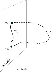
Figure 2: $W_{7}$ and $V_{7}$ have the five-brane worldvolume $W_{6}$ as a common boundary. The difference between them is that $W_{7}$ lies entirely in the 11D bulk $X$, whereas $V_{7}$ meets $X$ transversely from $Y$. The two components of $W_{6}$ serve here to emphasise that the five-brane worldvolume has to be a boundary; of course in practice $W_{6}$ can be connected.

Figure 3: Since $W_{7}$ and $V_{7}$ have the same boundary, they can be glued together to form a closed surface, $\partial V_{8}=W_{7}-V_{7}$.

A similar treatment is necessary for $\delta_{6}(U_{2})$, which is a delta-function on the five-brane worldvolume $W_{6}$. Denoting the inclusions again, abusively, by $\iota:W_{6}\hookrightarrow W_{7}$, we introduce a three-dimensional surface $U_{3}\subset W_{7}$ such that

$$\iota^{*}\delta_{7}(U_{3}) = \delta_{6}(U_{2})~{}.$$ (26)

Similarly to the above, its boundary is $U_{2}=W_{2}$ and we can glue it together with $W_{3}$ and call the thus constructed closed three-cycle $U_{3}-W_{3}=\partial U_{4}$.

We shall assume that the four-surface $U_{4}$ and the eight-surface $V_{8}$ actually exist. This means that

$$\partial(V_{8},W_{7}) = (V_{7},W_{6})$$ (27)

$$\partial(U_{4},U_{3}) = (W_{3},W_{2})$$ (28)

correspond to trivial classes in $H_{7}(Y,W_{7})$, resp. $H_{3}(Y,W_{7})$. However, this does not imply that the classes

$$[(V_{7},W_{6})] \in H_{7}(Y,W_{6})~{},$$ (29)

$${}[(W_{3},W_{2})] \in H_{3}(X,W_{6})$$ (30)

are trivial, because cycles modulo boundaries in $W_{6}$ is a larger space than that of cycles modulo boundaries in $W_{7}$.

Note also that this does not necessarily mean that spaces in which the above mentioned $H_{7}(Y,W_{7})$ and $H_{3}(Y,W_{7})$ homology groups are nontrivial are inconsistent backgrounds for wrapping branes. Rather than a restriction on cohomology of the background, this is a restriction on the configuration.

In this discussion, as we have already sketched in Fig. 2, the notation $W_{6}$ does not necessarily refer to an isolated brane, but rather can refer to a collection of them. The assumption of topological triviality made here is merely a statement of how these branes relate to each other. With this assumption, one cannot consistently describe an isolated five-brane in a compact space; there has to be at least one more brane present, such that there exists a homotopy between the two. This makes the homology class trivial, although the branes that we use to represent it are still physically nontrivial. Moving a five-brane worldvolume along this homotopy would then sweep out the worldvolume of the pertinent Dirac surface, $W_{7}$. In a noncompact space the extra brane worldvolume can be taken to infinity; this is indeed Dirac’s classical construction, sketched in Fig. 4. In other words, the brane charge has to have somewhere to flow.

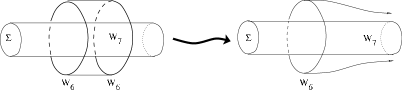
Figure 4: Brane worldvolumes $W_{6}$ wrapped around non-contractible cycles $\Sigma$ need to come in pairs, so that a connecting homotopy $W_{7}$ exists. In a noncompact space one of these can be taken to be at infinity, which produces the standard Dirac surface picture.

The only genuine restrictions on the model that we make are the assumptions that $W_{6}$ and $X$ have no boundaries. Note that this assumption does not imply that $W_{6}$ or $X$ has to be compact; open spaces without boundary, e.g. $\mathbb{R}^{11}$, are also acceptable. Even these restrictions could perhaps be relaxed by considering manifolds with edges, such as in extended topological quantum field theory.

We are now ready to write down the action in Dirac surface form:

$$S_{\mathrm{gauge}} = \int_{X}\frac{1}{2\kappa}~{}G\wedge*G+{T_{3}}G\wedge{\cal I}_{7}(R)-\int_{Y}\frac{1}{6\kappa}G\wedge G\wedge G$$

$$-\frac{1}{2}T_{6}\int_{(V_{8},W_{7})}\Big{(}G\wedge G-2\kappa T_{3}~{}{\cal I}_{8},~{}h\wedge\iota^{*}G\Big{)}$$

$$+\frac{T_{6}}{4}\int_{W_{6}}h\wedge*h+{T_{3}}\int_{U_{4}}G-\frac{T_{3}}{2}\int_{U_{3}}h~{}.$$

Here we have made use of the facts that $\partial(U_{4},U_{3})=(W_{3},W_{2})$ and that

$$-\int_{(W_{3},W_{2})}(C,b) = +\int_{(U_{4},U_{3})}(G,h)~{}.$$ (32)

As $U_{3}\subset W_{7}$ we may think of $U_{3}$ as a surface traversing through $W_{7}$, in contrast to $W_{3}$, which does not need to lie within $W_{7}$. One could perhaps think of $W_{3}$ as an electric and $U_{3}$ as a magnetic Dirac surface from the point of view of the self-dual theory on the five-brane.

We have also introduced in (3.1) the gravitational corrections ${\cal I}_{8},{\cal I}_{7}$ of Appendix A.5. The purely gravitational integral of ${\cal I}_{8}$, defined later in (A.5), is added here for convenience, although the evidence in its favour will surface later after calculating the contributions from integrals over $V_{8}$ in (51). The gravitational corrections lead to modifications in the definition of $\tilde{G}$ as well:

$$\tilde{G} \equiv {\mathrm{d}}\tilde{C}+\frac{1}{2}C\wedge G-\kappa T_{3}{\cal I}_{7}~{}.$$ (33)

The action (3.1) is essentially the same as the one proposed in Eq. (7.25) of Ref. [22]. The Dirac surfaces appear there through explicit delta-functions $\theta_{4}$ and $\theta_{7}$. The only differences with respect to [22] are in the identification of the physical membrane tension, and in the purely gravitational term $\int_{V_{8}}{\cal I}_{8}$, as opposed to the term $\int_{V_{7}}{\cal I}_{7}$ given in Ref. [22]. As the membrane tension in the equations of motion derived from the two actions is nevertheless the same, a factor of two difference in the integral over the membrane worldvolume reduces purely to a self-duality related convention.

Two surprising features of the action (3.1) are that there is no explicit $\tilde{C}$ dependence and that the coupling to $C$ and $b$ fields is not through the relative pair $(C,b)$. The former fact is a reflection of the locality of the action and the latter is a reflection of the nested structure of the geometry together with consequences of the self-duality of $h$.

We still need to show that this form of the action is independent of the choice of the Dirac surfaces. We will do so in Section 4.3.

Let us define the violated Bianchi identities in the bulk as

$${\mathbb{D}\,}(G,h) \equiv ({\mathrm{d}}G,\iota^{*}G-{\mathrm{d}}h)$$ (34)

$$= \Big{(}{\mathrm{d}}({\mathrm{d}}C),{\mathrm{d}}({\mathrm{d}}b)\Big{)}$$

$${\mathbb{D}\,}\tilde{G} \equiv {\mathrm{d}}\tilde{G}-\frac{1}{2}G\wedge G+\kappa T_{3}~{}{\cal I}_{8}$$ (35)

$$= {\mathrm{d}}({\mathrm{d}}\tilde{C})-\frac{1}{2}C\wedge{\mathrm{d}}G~{}.$$

The bulk equations of motion/Bianchi identities then take the form

$$\frac{1}{\kappa}~{}{\mathbb{D}\,}G = T_{6}\delta(W_{6})$$ (36)

$$\frac{1}{\kappa}~{}{\mathbb{D}\,}\tilde{G} = T_{3}\delta(U_{3}-\partial U_{4})+T_{6}h\wedge\delta(W_{6})$$ (37)

$$+T_{6}G\wedge\delta(V_{7}+\partial V_{8}-W_{7})~{}.$$

The last term in (37) actually drops out upon use of the surface relation $V_{7}+\partial V_{8}-W_{7}=0$, which we shall obtain shortly.

From the above discussion, we see that the proper global formulation of the theory as given in (3.1) guarantees the absence of awkward terms such as the last two terms in (2). The magnetic sources are then five-brane worldvolumes $W_{6}$, as expected, and the electric sources are the membrane worldvolumes $W_{3}$. Furthermore, membrane number can turn into worldvolume string flux through the coupling $h\wedge\delta(W_{6})$ with the correct multiplicity.

In writing down the action (3.1) we have actually used some facts that strictly speaking follow only from inspecting the equations of motion (36,37). In particular, we have used the fact that

$$T_{6}=-2\gamma~{}.$$ (38)

This result, which was anticipated in the considerations of Sec. 2.1, follows from taking the exterior derivative of (37) and comparing the terms proportional to $\delta(W_{6})$ with (19). The cancellation of the rest of the terms when taking the exterior derivative of (37) requires that the combination of surfaces $V_{7}+\partial V_{8}-W_{7}$ appearing in the first delta-function in (37) vanish identically. This then fixes the choice of the eight-dimensional Wess–Zumino term to be $\xi W_{8}=-(T_{6}/3)V_{8}$. Conversely, the presence of $W_{7}$ and $W_{8}$ in Eq. (4) requires that there exist some surface $V_{8}$ so that the boundary relation (27) holds.

3.2 The Hopf–Wess–Zumino term

Notice that in formulating the theory in this way, 12D data has to be included in the model from the very beginning. In the topologically trivial case, the original Wess–Zumino term therefore becomes

$$S_{\mathrm{WZ}} = \zeta\int_{W_{7}}C\wedge G+\frac{\xi}{2}\int_{W_{8}}G\wedge G$$ (39)

$$= \frac{T_{6}}{6}\int_{W_{7}-\partial V_{8}}C\wedge G$$

$$= \frac{T_{6}}{6}\int_{V_{7}}C\wedge G~{}.$$

Though the equalities here do not strictly hold in the topologically nontrivial case, the difference is of no consequence in the analysis performed above. Therefore, we can either start from the action that involves $W_{7}$ and $W_{8}$, and discover the topological constraint (27) when investigating the invariance properties of the full interacting theory or from the Wess–Zumino term (39) and the definition (25). This means that the Wess–Zumino term should be really seen as inherently 12D data.

This term is also quite closely related to the Hopf–Wess–Zumino term that was proposed in [29] to ensure correct anomaly cancellation in holography in the case of a stack of five-branes. As discussed in more detail in App. A.2, the field strength behaves near the five-brane worldvolume as $G=\kappa T_{6}\Omega_{{\scriptscriptstyle 4}}+\hat{G}$, so that when the smooth part vanishes, $\hat{G}=0$, the Wess–Zumino term becomes, using Eqs (43,49) to be found in the next section

$$S_{\mathrm{WZ}} = \frac{\kappa T_{6}^{3}}{6}\int_{V_{7}}\Omega_{3}\wedge\Omega_{4}=\frac{2\pi}{6}\int_{V_{7}}\Omega_{3}\wedge\Omega_{4}~{}.$$ (40)

For $V_{7}=S^{7}$ this is precisely the Hopf-invariant of a class in $\pi_{7}(S^{4})$ suggested in [29] for the anomaly deficit $c(G)-c(H)=1$. Though this involves extrapolating the gauge group to a single brane configuration, the above should serve as a microscopic supergravity derivation of the interaction term conjectured in [29] on grounds of duality principles.

4 Consistency conditions, gauge and charge lattices

In this section we will check that the Dirac surface form of the action is well-defined modulo $2\pi$, and will derive quantisation conditions for fluxes, tensions, and large gauge transformations.

4.1 Dirac quantisation

We first show that the fluxes $G$, $(G,h)$ and $\tilde{G}$ are quantised in a certain sense, even if not all of them are closed classes in cohomology. This will be sufficient to show that the large gauge transformations take their values in a certain integer lattice.

The first check on the partition function is to see what happens when one transports a membrane worldvolume adiabatically around a five-brane source worldvolume as sketched in Fig. 5. Let us suppose first that the membrane and the five-brane are well separated and that the former does not end on the latter. This leads to the standard Wu–Yang derivation [30] of the Dirac quantisation condition [31]. The phase of the membrane coupling, when transported along a curve $\Sigma_{4}$, is

$$T_{3}\int_{W_{3}^{\mathrm{fin}}}C-T_{3}\int_{W_{3}^{\mathrm{ini}}}C=T_{3}\int_{\Sigma_{4}}G\stackrel{{\scriptstyle!}}{{=}}2\pi~{}.$$ (41)

This tells us that the integrals of $\frac{T_{3}}{2\pi}G$ are integers when calculated over surfaces that neither have a boundary nor intersect the five-brane source worldvolume itself,

$$\left[\frac{T_{3}}{2\pi}G\right]\in H^{4}(Y,\mathbb{Z})\ .$$ (42)

If we view $\Sigma_{4}=\partial D_{5}$ as a boundary of a five-disc and also use the equation of motion (17), we obtain the standard Dirac quantisation condition

$$\kappa~{}T_{3}T_{6}=2\pi~{}.$$ (43)

Figure 5: The membrane worldvolume $W_{3}$ can be transported around a five-brane worldvolume $W_{6}$ along a closed path $\Sigma_{4}$. This path can be filled in to form a disc $D_{5}$ which the five-brane worldvolume $W_{6}$ intersects once transversely.

It is also possible to use this same argument even in cases where the membrane ends on the five-brane; this yields a quantisation condition for the tension $T_{2\hookrightarrow 6}$ of the self-dual strings in the five-brane worldvolume. The argument is more subtle, however, because of the self-duality. It is useful to think of any string source $W_{2}\subset W_{6}$ as a sum of an electric and a magnetic source, which are interchanged by self-duality. They are at the boundary of a bulk membrane worldvolume $W_{3}$, which we consequently have to move in an adiabatic fashion along with the attached worldvolume strings as well, cf. Fig. 6. The part of the action (2) that is affected by the adiabatic argument is then

$$-T_{3}\int_{(W_{3},W_{2})}(C,\frac{1}{2}b)$$ (44)

Since membranes are not self-dual, the adiabatic argument yields the change of phase

$$T_{3}\int_{(W_{3},W_{2})_{\mathrm{fin}}}(C,b)-T_{3}\int_{(W_{3},W_{2})_{\mathrm{ini}}}(C,b)=T_{3}\int_{(\Sigma_{4},\Sigma_{3})}(G,h)\stackrel{{\scriptstyle!}}{{=}}2\pi~{}.$$ (45)

Note that the factor of ${\textstyle{\frac{{\scriptstyle 1}}{\scriptstyle 2}}}$ has now vanished as anticipated above. Here $(\Sigma_{4},\Sigma_{3})$ describes the path along which we transport the combined membrane – string system, cf.  Fig. 7.

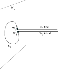
Figure 6: Since the worldvolume strings $W_{2}$ are the membranes’ endpoints, moving one means moving the other.

Figure 7: $\Sigma_{3}$ is the path that the string worldvolume $W_{2}\subset W_{6}$ adiabatically traverses, and $\Sigma_{4}$ is that traversed by the membrane worldvolume. $\Sigma_{4}$ is therefore the surface of a (hollow) cylinder that ends on $\Sigma_{3}$ in $W_{6}$. If we fill in the latter to make a 4-disc $D_{4}$ and add this to $\Sigma_{4}$ we get a capped cylinder, which can then be filled in to yield a solid cylinder $D_{5}$.

On the level of cohomology, the above considerations mean that the class $\frac{T_{3}}{2\pi}(G,h)$ is integral,

$$\left[\frac{T_{3}}{2\pi}(G,h)\right]\in H^{4}(Y,W_{6};\mathbb{Z})\ .$$ (46)

We can further fill in the cylinder shown in Fig. 7 so that $(\Sigma_{4},\Sigma_{3})=\partial(D_{5},D_{4})$, and we can use the equation of motion (19). Now it is important to notice that the integral

$$\int_{D_{5}}\delta_{X}(W_{6})=0$$ (47)

vanishes because the five-volume $D_{5}$ meets the five-brane worldvolume $W_{6}$ only along a dimension-four surface $D_{4}$. Indeed, the current $\delta_{X}(W_{6})$ involves differentials along the five transverse directions of the five-brane worldvolume, whereas the integration domain $D_{5}$ only includes one of these directions. We get therefore a quantisation condition that involves only terms relating to the worldvolume string and the membrane,

$$T_{2\hookrightarrow 6}T_{3}=2\pi~{}.$$ (48)

Now recall that $T_{2\hookrightarrow 6}=T_{3}/T_{6}$ was related to the bulk tensions so that finally we have

$$(T_{3})^{2} = 2\pi T_{6}~{}.$$ (49)

We will rederive this in different ways later on. The above argument also serves to elucidate the relationship between relative homology and Dirac surfaces. There are two observations to be made at this point:

• The results (43) and (49) follow also by requiring that the action (3.1) remain well-defined modulo $2\pi$ when we distort $U_{4}$ or $U_{3}$ by a surface without a boundary. Here, in order to understanding the factor of ${\textstyle{\frac{{\scriptstyle 1}}{\scriptstyle 2}}}$ in front of the last term in (3.1), one must remember that that the integral involves only half of the naïvely apparent fluxes by virtue of the self-duality of $h$.

• The result (48) also follows from the quantisation of dyonic charges as discussed in [33]. There, it was noted that, in $D=4k+2$ dimensions and for Lorentzian signature, the generalised Dirac–Schwinger–Zwanziger quantisation condition [34, 35] involves a relative plus-sign, i.e. $e_{1}g_{2}+e_{2}g_{1}=2\pi\kappa$. In the case of a self-dual flux we thus have an extra factor of two, and so $e_{1}e_{2}=\pi\kappa$.

Let us finally turn to the membrane flux $\tilde{G}$. Collecting all the $V_{8}$ dependent terms in the action we get

$$\int_{V_{8}}\cdots = -T_{6}\int_{V_{8}}{\mathrm{d}}\tilde{G}+T_{6}\int_{V_{8}}{\mathbb{D}\,}\tilde{G}$$ (50)

$$= -T_{6}\int_{\partial V_{8}}\tilde{G}+\kappa T_{6}T_{3}\int_{V_{8}}\delta_{Y}(U_{4})+\kappa(T_{6})^{2}\int_{V_{8}}h\wedge\delta_{Y}(V_{7})~{}.\ \$$ (51)

The last term is at least naïvely trivial, because integrals over $\delta_{Y}(V_{7})$ could possibly contribute only when taken over domains that include the five normal directions of $V_{7}$, whereas $V_{8}$ only includes one of them. This term may play a rôle if we consider more complicated self-intersections of $V_{7}$ and $V_{8}$, but even then, assuming that ${\mathrm{d}}h=0$ and $\partial(V_{8}\cap V_{7})=0$ and using the above-found relations for the tensions, we see that this term as well as the penultimate term contribute only integer multiples of $2\pi$. The $V_{8}$ dependence of the “$\mathop{\rm mod}\nolimits 2\pi$”-action comes therefore entirely from the membrane flux through the surface $\partial V_{8}=W_{7}-V_{7}$.

It does not make sense to require that the membrane flux $\tilde{G}$ be a class in integral cohomology, since it is not even closed when $G\wedge G$ or ${\cal I}_{8}$ are nontrivial. However, we have already seen above that even fluxes that are not generically closed, such as $h$, may nevertheless be associated to a quantisation condition in the full interacting theory, such as Eq. (46). Furthermore, we must be able to show that the action (3.1) is independent of the choice of the Dirac surface $V_{8}$. This is actually possible, and the proof proceeds in two steps which we relegate to subsequent sections. It turns out that the ${\mathrm{d}}\tilde{C}$ and the $\frac{1}{2}G\wedge G-\kappa T_{3}{\cal I}_{7}$ parts can be discussed independently: the treatment of the former gives rise to quantisation of the six-form gauge transformations, as we will see at the end of Sec. 4.2; the latter will require a full analysis of deformations of the Dirac surfaces, which we will make in Sec. 4.3.

4.2 The lattice of large gauge transformations

The fact that the integral of $T_{3}G$ over any four-sphere is an integer multiple of $2\pi$ means that the allowed large gauge transformations relating the values of the gauge field on different hemispheres must also lie in integral cohomology,

$$\left[\frac{T_{3}}{2\pi}\Lambda_{3}\right] \in H^{3}(Y,\mathbb{Z})~{}.$$ (52)

In more detail, we may divide an integral of $G$ over $S_{4}$ into integrals over 4-discs $D,D^{\prime}$ where the field strength can be trivialised to $dC,dC^{\prime}$. The gauge fields on $D$ and $D^{\prime}$, with $\partial D=\partial D^{\prime}=S^{3}$, differ by a gauge transformation, $C^{\prime}=C+\Lambda$, so that

$$\int_{S^{4}}G=\int_{D^{\prime}}{\mathrm{d}}C^{\prime}+\int_{D}{\mathrm{d}}C=\int_{S^{3}}C^{\prime}-C=\int_{S^{3}}\Lambda~{}.$$ (53)

Similarly, the flux quantisation condition (46) implies

$$\left[\frac{T_{3}}{2\pi}(\Lambda_{3},\lambda_{2})\right] \in H^{3}(Y,W_{6};\mathbb{Z})~{}.$$ (54)

In Eqs (52) and (54) we have used the fact that the 4-form classes $[T_{3}G/2\pi]$ extend as integral classes from $X$ to $Y$, as was mentioned in the beginning of Sec. 4. The large gauge transformations (54) take values in the relative cohomology of the pair $(Y,W_{6})$ rather than in that of the pair $(Y,W_{7})$ because the flux quantisation condition (46) did not involve the Dirac surface $W_{7}$ in any way.

A perhaps more direct way to see this is to notice that the worldvolume couplings

$$\int_{(W_{3},W_{2})}(C,b)$$ (55)

remain invariant modulo $2\pi$ only if the above quantisation conditions apply. The action (3.1) actually involves a slightly different combination of these terms, as pointed out in Eq. (44), but as the discussion there implied, the coupling that takes self-duality properly into account is indeed of the form (55).

Even if there is no direct coupling to $\tilde{C}$ we will still need to restrict the large six-form gauge transformations to the lattice

$$\left[\frac{T_{6}}{2\pi}\Lambda_{6}\right] \in H^{6}(Y,\mathbb{Z})~{},$$ (56)

as was promised in the discussion below Eq. (51). To see this, consider deforming the surface $\partial V_{8}$ by inserting a handle without boundaries, such as sketched in Fig. 8. It may well then happen that the gauge field $\tilde{C}$ has to undergo a large gauge transformation $\Lambda_{6}$ somewhere around the neck of the deformation, say at the sphere $S^{6}$. More concretely, let us cut out from the original surface $\partial V_{8}$ some small 7-disc $D_{7}$ with boundary $S^{6}$. We may then deform the cut surface by pulling the $S^{6}$ boundary some small distance away form its original location on the surface $\partial V_{8}$ as sketched in Fig. 8. We may next glue along the boundary $S^{6}$ a handle $\Sigma_{7}$. If it happens that the 6-form gauge field on the original surface $\tilde{C}_{0}$ and on the handle $\tilde{C}_{1}$ differ by a large gauge transformation $\tilde{C}_{0}-\tilde{C}_{1}=\Lambda_{6}$ then the term

$$-T_{6}\int_{\partial V_{8}}{\mathrm{d}}\tilde{C}$$ (57)

in the $V_{8}$-part of the action (51) is subject to a shift by the amount

$$-T_{6}\int_{\partial V_{8}-D_{7}}{\mathrm{d}}\tilde{C}_{0}-T_{6}\int_{\Sigma_{7}}{\mathrm{d}}\tilde{C}_{1}=T_{6}\int_{\partial D_{7}}\tilde{C}_{0}-T_{6}\int_{\partial\Sigma_{7}}\tilde{C}_{1}=T_{6}\int_{S^{6}}\Lambda_{6}\ .$$ (58)

Requiring the theory to be insensitive to this deformation gives rise to the integrality condition (56) above.

Figure 8: Deforming $\partial V_{8}$, and therefore $W_{7}$ (or $V_{7}$) by adding a handle $\Sigma_{7}$, after cutting out an original disk $D_{7}$. The gauge field $\tilde{C}$ undergoes a large gauge transformation somewhere in the neck, for instance around the sphere $S^{6}$. The handle may also contain noncontractible three-spheres that have an influence on the M-theory gauge algebra.

Notice that it is important that the cut surface boundary modelled here by $S^{6}$ may be anywhere in space. In fact, had we restricted ourselves to comparing the values of the 6-form gauge fields only on the original Dirac surfaces $W_{7}$ and $V_{7}$, the comparison would have to be made at the joint boundary of $W_{7}$ and $V_{7}$, i.e. on the original five-brane worldvolume $W_{6}$. This would then complicate the discussion that we shall give of the gauge algebra in Sec. 5. Indeed, were the gauge transformations in this discussion always localised on $W_{6}$, then by $\iota^{*}\Lambda_{3}={\mathrm{d}}\lambda_{2}$, the wedge product of two 3-form transformations would give rise to a 6-form transformation $\Lambda_{6}=\Lambda_{3}^{\prime}\wedge\Lambda_{3}$ that is a trivial class when pulled back to $W_{6}$, and consequently we would not obtain any constraint on the 6-form gauge transformation lattice.

In conclusion, even though the 7-form flux does not itself need to be closed or integral, the transition functions of the 6-form gauge field, and consequently the 6-form gauge transformations, need to be integral (56) in order to guarantee that the action is well-defined.

4.3 Dependence on Dirac surfaces

Guaranteeing independence of the theory from the choice of the surfaces $Y$ and $V_{8}$ under shifts by closed surfaces boils down to requiring that

$$\left[\frac{1}{3!~{}\kappa}G^{3}\right]\quad\text{ and }\quad\left[\frac{T_{6}}{2!}G^{2}\right]$$ (59)

are integral. The first of these two integrality conditions was found, in essentially the same way, in Ref. [36]; see also the appendix in Ref. [37]. Using (42) this means

$$\frac{(2\pi)^{2}}{\kappa}=(T_{3})^{3}\quad\text{ and }\quad 2\pi T_{6}=(T_{3})^{2}~{},$$ (60)

which is equivalent to requiring that (43) and (49) hold. The treatment of these formulas in the face of gravitational corrections would require a discussion of anomalies.

These quantisation rules are necessary, but not quite sufficient to guarantee the independence of the theory from the choices of Dirac surfaces that we have made, because they only guarantee the independence from the choice of the surfaces $Y$ and $V_{8}$. Showing independence also from the choices of $V_{7}$ and $W_{7}$, is further complicated because the Bianchi identity for $h$ given in (20) is obviously not of the kind that we see in standard de Rham cohomology. This issue can be settled by checking what happens to the action when we shift all of the Dirac surfaces arbitrarily outside the sources (19,20,36,37). This is essentially an exercise in 12D Euclidean geometry, but we give here an outline in algebraic form.

Quite generally, if we deform $W$ smoothly to $W^{\prime}$, we sweep out thereby a surface whose boundary is exactly $W^{\prime}-W$ (cf. Fig. 9). As some surfaces lie by definition within the worldvolumes of others, such as $U_{3}\subset W_{7}$, moving the latter moves automatically the former as follows:

$$Y^{\prime}=Y+\partial Z \Longrightarrow V_{7}^{\prime}=V_{7}+\partial Z_{8}$$ (61)

$$W_{7}^{\prime}=W_{7}+\partial D_{8} \Longrightarrow U_{3}^{\prime}=U_{3}+\partial D_{4}\ .$$ (62)

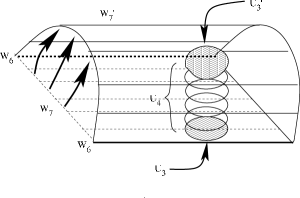
Figure 9: Since $U_{3}$ was defined as a subset of $W_{7}$ whose boundary is the string worldsheet $W_{2}$, varying $W_{7}$ means varying $U_{3}$ while keeping the boundary fixed. Under smooth variations $U_{3}$ sweeps out a volume $U_{4}$.

Apart from these standard Dirac surfaces, in the context of relative cohomology we have also to deal with “Dirac surfaces for Dirac surfaces” such as $U_{4}$ and $V_{8}$. These are volumes whose boundaries consist partially of physical branes and partially of Dirac surfaces. As we do not know a priori what is physical and what is not, we will have to vary these volumes arbitrarily

$$V_{8}^{\prime}=V_{8}+T_{8}$$ (63)

$$U_{4}^{\prime}=U_{4}+T_{4} \ .$$ (64)

The total shift in the action under (61–64) is

$$\frac{T_{6}}{2}\int_{D_{8}-T_{8}-Z_{8}}G\wedge G+2\pi\int_{T_{8}}{\cal I}_{8}+{T_{3}}\int_{T_{4}-D_{4}}G+\frac{T_{3}}{2}\int_{(D_{4},\partial D_{4})}(G,h)~{}.$$

(65)

The last term in (65) is trivial, because it is a pairing of a relative cohomology class with a trivial homology class; this is why the factor of ${\textstyle{\frac{{\scriptstyle 1}}{\scriptstyle 2}}}$ here does not cause any further change in the result. Naïvely, it would seem to be necessary to require the other integration domains to be empty. However, since it is sufficient to require these terms to integrate to multiples of $2\pi$, we need these domains only to be without boundary, by virtue of the integrality rule (42):

$$\partial(-D_{8}+T_{8}+Z_{8}) = 0~{},$$ (66)

$$\partial T_{8} = 0~{},$$ (67)

$$\partial T_{4}-\partial D_{4} = 0~{}.$$ (68)

Consequently, the integrality conditions (42) guarantee that the ambiguity in the choice of Dirac surfaces indeed boils down to shifts in the action by integer multiples of $2\pi$, as required. Note that for this we need, in addition to the integrality of $G$ in (42), to require also that

$$[{\cal I}_{8}]\in H^{8}(Y,\mathbb{Z})~{}.$$ (69)

This condition is already familiar, however, from the membrane tadpole cancellation arguments of [38, 39].

We can look at the above relationships between shifts in essentially two ways. The first is by checking that the relationships (27,28) found between Dirac surfaces guarantee that the constraints (66–68) are satisfied. This would mean that the Dirac surface form of the action (3.1) is a good representation of the original form (1–4) of the action. This is indeed the case:

Proof: The fact that $T_{8}$ cannot have a boundary is guaranteed by the fact that $W_{7}$ and $V_{7}$ fix the cobordism class of $V_{8}$ once and for all. The requirement $\partial(-D_{8}+T_{8}+Z_{8})=0$ follows from requiring that $-W_{7}+V_{7}-\partial V_{8}$ be preserved under deformations. And $\partial T_{4}=\partial D_{4}$ follows from the construction $\partial U_{4}=U_{3}-W_{3}$, which actually guarantees even that $T_{4}=D_{4}$.

The second way of looking at this is to note that one can show that the relations (27) and (28) arise from (65), so that (3.1) carries enough information to tell us which combinations of the many surfaces ($U_{3},U_{4},W_{7},V_{8},X,Y$) are actually physical, and which ones are mere artifacts of the description, i.e.  Dirac surfaces:

Proof: The two last terms of (65) betray that the shift

$$\delta(U_{4},U_{3}) = (D_{4},\partial D_{4})$$

is closed under $\partial$. This tells us that any equation $\partial(U_{4},U_{3})=(W_{3},W_{2})$ for a fixed representative of a homology class

$$[(W_{3},W_{2})]\in H_{3}(Y,W_{7};\mathbb{Z})$$ (70)

is invariant under these shifts. As $\partial T_{8}=0$ we see that we are allowed to modify $V_{8}$ by deformations that do not change the boundary. This fixes $V_{8}$ to be any representative of a given cobordism class in $Y$, i.e. $\partial V_{8}=\text{{\em something fixed}}$. On the other hand, the equation $\partial(-D_{8}+T_{8}+Z_{8})=0$ states that the equation $W_{7}-V_{7}+\partial V_{8}=\text{{\em anything fixed}}$ remains invariant under all deformations. This means that the cobordism class of $V_{8}$ is actually given by $W_{7}-V_{7}$, and that $W_{7}$ and $V_{7}$ have a common boundary. If we call this boundary $W_{6}$, we find $\partial(V_{8},W_{7})=(V_{7},W_{6})$.

This leads us back to (28) and (27).

5 The Symmetry Algebras

The quadratic tension rule $(T_{3})^{2}=2\pi T_{6}$ can be derived also from the M-theory gauge algebra. To see exactly how, let us look again at the gauge algebra mentioned in Sec. 1 and in Eqs (13–16), extended now into the 12D space $Y$

$$\delta_{\cal G}(C,b) = (\Lambda_{3},\lambda_{2})$$ (71)

$$\delta_{\cal G}\tilde{C} = \Lambda_{6}+\frac{1}{2}\Lambda_{3}\wedge C~{}.$$ (72)

The gauge transformations satisfied ${\mathrm{d}}\Lambda_{3}={\mathrm{d}}\Lambda_{6}=0$ and $\iota^{*}\Lambda_{3}={\mathrm{d}}\lambda_{2}$. We have already learned in Eqs (52) and (54) that the large gauge transformations live on a lattice

$$\left[\frac{T_{3}}{2\pi}(\Lambda_{3},\lambda_{2})\right] \in H^{3}(Y,W_{6};\mathbb{Z})$$ (73)

$$\left[\frac{T_{6}}{2\pi}\Lambda_{6}\right] \in H^{6}(Y,\mathbb{Z})~{}.$$ (74)

We distinguish here between a cohomology class, e.g. $[\Lambda_{6}]$, and its representative $\Lambda_{6}$. These gauge transformations satisfy a noncommutative algebra, where the only nontrivial bracket is

$$[\delta_{3}^{\prime},\delta_{3}] = \delta_{6}~{},$$ (75)

with structure constants such that $\Lambda_{6}=\Lambda_{3}^{\prime}\wedge\Lambda_{3}$. This leads us to the derivation of the tension rule (49) as presented in [40]: namely that since $\Lambda_{3}^{\prime}\wedge\Lambda_{3}$ has to belong to the same lattice as $\Lambda_{6}$, we get

$$\frac{T_{3}}{2\pi}\chi\wedge\frac{T_{3}}{2\pi}\chi^{\prime} \stackrel{{\scriptstyle!}}{{=}} \frac{T_{6}}{2\pi}\psi$$ (76)

for some representatives of the integral elements $[\chi],[\chi^{\prime}]\in H^{3}(Y,\mathbb{Z})$, $[\psi]\in H^{6}(Y,\mathbb{Z})$. This holds if and only if

$$T_{3}^{2} = 2\pi~{}T_{6}~{}.$$ (77)

For illustration, see Fig. 8: $\chi$ and $\chi^{\prime}$ could be the volume forms of two independent 3-spheres or 3-tori in the handle $\Sigma_{7}$, one of which, $S^{3}$, is indicated in the picture. It is quite remarkable that the quantisation condition (49) arises in this way. Our treatment of this derivation adds to that presented in [40] a consistent treatment of global gauge transformations that was not addressed there.

Though we have not investigated the intricacies of diffeomorphisms and anomaly cancellation in this paper, it is of interest to see how the gauge symmetry algebra fits together with the diffeomorphism algebra. Using notation from App. A.3 the diffeomorphism transformations act on the various fields according to

$$\delta_{\cal D}(C,b) = \frac{T_{3}}{2\pi}~{}\Big{(}{\mathrm{d}}\Omega_{2}^{(1)},~{}0\Big{)}$$ (78)

$$\delta_{\cal D}\tilde{C} = \frac{T_{6}}{2\pi}~{}\Omega_{6}^{(1)}+\frac{1}{2}{\mathrm{d}}\Omega_{2}^{(1)}\wedge\frac{T_{3}}{2\pi}~{}C~{}.$$ (79)

These rules follow, as explained above and in App. A.3, from requiring that $\tilde{G}$ be invariant and that $G$ look like $\kappa T_{\scriptscriptstyle 6}~{}\Omega_{\scriptscriptstyle 4}$ near the five-brane. As $b$ is purely worldvolume data, it is natural to keep it inert under these diffeomorphisms. From the five-brane worldvolume point of view, these transformations reduce to worldvolume diffeomorphisms and SO(5) gauge transformations on the normal bundle as suggested in the pull-back of the bulk tangent bundle $T_{\scriptscriptstyle X}|_{{\scriptscriptstyle W}}=T_{\scriptscriptstyle W}\oplus NW$. The difference between large and small diffeomorphisms is that the former [41, 42] preserve the normal bundle $NW$ and $\Omega_{\scriptscriptstyle 2}^{{\scriptscriptstyle(1)}}$ is globally defined, whereas in the latter only $\delta\Omega_{\scriptscriptstyle 3}$ exists globally.

The transformation functionals are not inert under repeated diffeomorphism transformations, but instead one finds the non-trivial contribution

$$\delta_{\cal D}^{(2)}\tilde{C} = \frac{T_{6}}{2\pi}~{}{\mathrm{d}}\Big{(}\Omega_{5}^{(2)}+\frac{1}{2}\Omega_{2}^{(1)}\wedge{\mathrm{d}}\Omega_{2}^{(1)\prime}\Big{)}~{}.$$ (80)

We conclude that iterated diffeomorphisms reduce to gauge transformations $\delta_{\cal D}^{{\scriptscriptstyle(2)}}=\delta_{\cal G}$ with the parameter

$$\Lambda_{6} = \frac{T_{6}}{2\pi}~{}{\mathrm{d}}\Big{(}\Omega_{5}^{(2)}+\frac{1}{2}\Omega_{2}^{(1)}\wedge{\mathrm{d}}\Omega_{2}^{(1)\prime}\Big{)}~{}.$$ (81)

Also, diffeomorphisms and gauge transformations do not commute, but

$$[\delta_{\cal D},\delta_{3}] = \delta_{6}~{},$$ (82)

where $\Lambda_{\scriptscriptstyle 6}=({T_{\scriptscriptstyle 3}}/{4\pi})~{}{\mathrm{d}}\Omega_{\scriptscriptstyle 2}^{{\scriptscriptstyle(1)}}\wedge\Lambda_{\scriptscriptstyle 3}$. This shows, therefore, that the algebra (75) remains valid also for the direct sum of transformations

$$\delta = \delta_{\cal D}+\delta_{\cal G}~{}$$ (83)

of diffeomorphism and gauge transformations. The real form of this algebra is a truncation of the algebras found in Refs [43, 12, 44, 45, 46], which include for instance $E_{11}$ and hyperbolic Kač–Moody algebras. The integral forms of these algebras arise in quantum string theory in ten dimensions as U-duality.

6 Discussion

Let us start by recapitulating our results. The correct, though not manifestly gauge invariant action is

$$S_{\mathrm{gauge}} = ~{}\frac{1}{\kappa}\int_{X}\frac{1}{2}~{}G\wedge*G-\frac{1}{6}~{}C\wedge G\wedge G+\kappa T_{3}G\wedge{\cal I}_{7}$$

$$\qquad\qquad\qquad+\frac{T_{6}}{6}\int_{V_{7}}C\wedge G+2\pi\int_{V_{8}}{\cal I}_{8}$$

$$+\frac{T_{6}}{2}\int_{W_{6}}\left(\frac{1}{2}h\wedge*h-h\wedge{\iota^{*}}C\right)-T_{3}\int_{W_{3}}C+\frac{T_{3}}{2}\int_{W_{2}}b~{}.$$

In writing the action in this form, it has to be understood that $V_{7}$ is related to $W_{7}$ and $W_{8}$ through Eq. (27). Using the same relation, the last terms of the first and the second line combine to integrals over $V_{7}$ as well. We choose nevertheless to leave an explicit $V_{8}$ integral here; a purely gravitational shift in the action does not change its gauge symmetry properties, but will be significant in any future discussion of diffeomorphism symmetry and anomalies.

Two features in particular merit to be pointed out: First, there is no explicit magnetic $\tilde{C}$ coupling. Secondly, there is a relative factor of two in the membrane tension and the worldsheet string tension. This latter fact is related to the self-duality of the closed worldsheet string theory.

The above action can be rewritten using essentially only Stokes’ theorem in the manifestly gauge invariant form

$$S_{\mathrm{gauge}} = \int_{X}\frac{1}{2\kappa}~{}G\wedge*G+{T_{3}}G\wedge{\cal I}_{7}(R)-\int_{Y}\frac{1}{6\kappa}G\wedge G\wedge G$$

$$-\frac{1}{2}T_{6}\int_{(V_{8},W_{7})}\Big{(}G\wedge G-2\kappa T_{3}~{}{\cal I}_{8},~{}h\wedge\iota^{*}G\Big{)}$$

$$+\frac{T_{6}}{4}\int_{W_{6}}h\wedge*h+{T_{3}}\int_{U_{4}}G-\frac{T_{3}}{2}\int_{U_{3}}h~{}.$$

The integration domains here are related to the physical branes by

$$\partial(U_{4},U_{3})=(W_{3},W_{2}),\quad\partial(V_{8},W_{7})=(V_{7},W_{6}),\quad\text{and}\quad\partial Y=X~{}.$$

As was shown in Sec. 4.3 this information can actually be recovered from the action (6) as well.

We conclude that the original action $S\mathop{\rm mod}\nolimits 2\pi$ in Eq. (6) should be, as far as it is possible to express in terms of standard differential forms, the physically correct coupling of brane and bulk dynamics.

More precisely, we have found the following:

• We have presented a novel globally well-defined form of the action, collected in Eq. (6) above, thereby elucidating how five-branes should be embedded into the 11D supergravity background. Though this action involves spurious surfaces, the standard physical branes emerge as solutions of “topological” equations of motion. The way in which these spurious surfaces appear poses restrictions on any putative 12D theory on whose boundary M-theory could arise.

• We have also shown how the M-theory gauge algebra remains valid globally. This leads to the well-known [47, 37, 40, 44] constraints on the brane tensions

  $$\kappa~{}T_{3}T_{6} = 2\pi\hbar~{},$$ (86)

  $$(T_{3})^{2} = 2\pi\hbar~{}T_{6}~{}.$$ (87)

  This was checked in Eqs (49,60,77) independently using Wu–Yang type arguments, and also by requiring independence with respect to the positioning of the Dirac surfaces.

• As a by-product, we derived an Abelian counterpart (39) of the Hopf–Wess–Zumino term proposed in [29]. It arises naturally in requiring gauge invariance.

• We identified the five-brane charges as integrals of classes in the relative cohomology of $(X,W_{6})$. Similar conclusions were made already in Refs [9, 48] where D2 and D0-branes in WZW models were discussed. In trying to define charges for these Chern–Simons type systems, most previous candidates have failed to be either localised, or quantised, or gauge invariant [49, 50, 51]. On the level of fluxes, relative cohomology seems to provide the right classification of physical states and a resolution to these difficulties.

6.1 No new degrees of freedom

The inclusion of Wess–Zumino terms defined on $W_{7}\subset X$ might appear surprising, as they do not correspond to physical M-branes. Adding these geometric objects is nevertheless perfectly consistent with what we know about M-theory as long as they do not introduce new degrees of freedom. Their “worldvolume” theories, of which we have seen only a part, could perhaps turn out to be gravitational or topological theories in nature, whose dynamical degrees of freedom have a holographic description on their boundary, that is to say on the five-brane.

As these additions are expressible purely as integrals over $V_{7}$, we should now discuss the differences of these Dirac surfaces and in particular the rôle that this boundary $V_{7}$ plays in more detail.

As we have discovered, the word “boundary” may stand for many things in an analysis involving relative cohomology. The Dirac surface here is actually the relative class $(V_{8},W_{7})$ and the physical brane worldvolume is the class $(V_{7},W_{6})$. However, all the modifications that we have actually made to the standard M-theory action in eleven dimensions involve $V_{7}$ rather than one of the pair $(V_{8},W_{7})$. Nevertheless, $V_{7}$ is just a Dirac surface for the five-brane, but it has an interesting origin: most conspicuously, perhaps, $V_{7}$ extends out of the 11D spacetime $X$ of M-theory, and is therefore inherently an object of a 12D theory. It is physical in the sense that the lift of the Bianchi identity (17) to twelve dimensions, as given in (25), involves a delta-function onto $V_{7}$, so that the five-brane worldvolume is essentially just the dimensional reduction of this to eleven dimensions. Let us discuss next what this might mean.

There is a final superalgebra in twelve dimensions [52] that still has 32-component spinorial generators. This 12D superalgebra differs crucially from the 11D one in that the signature of the metric is $10+2$ rather than Minkowskian and that it does not contain Poincaré generators. The absence of Poincaré generators in the rigid 12D algebra is suggestive of a topological theory with $\mathop{\rm SO}\nolimits(10,2)$ invariance. This may suggest that the theories in twelve and eleven dimensions could be related by some form of Holography, which would preemptively resolve the apparent difficulties with the appearance of new degrees of freedom.

Furthermore, the 12D superalgebra contains in particular a self-dual 6-form central charge. It is therefore conceivable that $V_{7}$ could appear as a BPS state in that theory. This would be natural as the 6-form central charge reduces exactly to a five-brane charge under (double) dimensional reduction. This reduction does not give rise to an 11D 6-form central charge precisely because of the self-duality condition: we can always choose to work in a basis where the 12D 6-form involves the twelfth, compact coordinate. This emphasises further the fact that the 12D formulation does not import new degrees of freedom to the theory, since even on the level of representations of the respective superalgebras the 5-form and the 6-form central charges describe the same number of dynamical degrees of freedom.

6.2 Open questions

In dealing with smooth manifolds with boundaries, the boundary operator is nilpotent $\partial^{2}=0$. Nevertheless, much of the interesting structure of 11D formulations of M-theory is related to the Hořava–Witten boundaries of $X$, which we have not addressed here at all. They could be included in the discussion replacing, in principle, smooth manifolds with manifolds with edges and vertices. This would take us into the realm of extended topological quantum field theory, possibly along the lines of Ref. [54]. An early indication of this is perhaps the fact that we could think of the five-brane worldvolume as the edge in the manifold $W_{7}-V_{7}$ sketched in Fig. 2, thus avoiding the need to assume that the “Dirac surface for Dirac surfaces” $V_{8}$ exist.

Diffeomorphism symmetry and its violations by five-brane solutions play a pivotal rôle in anomaly cancellation. Analysing this requires understanding fully the behaviour of the $C$-field solution near a five-brane worldvolume [20]. In addressing these issues, Wess–Zumino terms built out of worldvolume scalars are crucial [55]. Another interesting question is when exactly are the extensions of worldvolume fields to Dirac surfaces obstructed. In the case of the worldvolume field $h$ this issue can be settled using Hodge decomposition, but it becomes more subtle in the case of the worldvolume scalars.

A formulation of the theory in terms of non-dynamical Dirac surfaces may involve higher dimensional physical states, such as BPS states, as long as these states reduce to the same number of physical states as that expected in the original lower dimensional formulation of the theory. The problem is then to find a mechanism to guarantee that this always happens. As was pointed out in Sec. 3.2 and in [29], the term $\int C\wedge G$ on a classical solution calculates the winding number of $V_{7}$ on $S^{4}$. An obvious candidate for the holographic dual of the five-brane worldvolume theory on $V_{7}$ could therefore be a topological quantum field theory based on the group $\pi_{7}(S^{4})=\mathbb{Z}\oplus\mathbb{Z}_{12}$. The idea of formulating M-theory as a holographical theory has surfaced earlier in a different context, for instance in [56].

Acknowledgements:

We thank T. Damour, B. Julia and R. Minasian for helpful discussions. We also wish to acknowledge the hospitality of the Institut des Hautes Études Scientifiques and of the Isaac Newton Institute at times during the course of this work. J.K. acknowledges the financial support provided through the European Community’s Human Potential Programme under contract HPRN-CT-2000-00131 Quantum Spacetime.

Appendix A Appendices

A.1 Currents and delta-functions

Given a subsurface $\Sigma$ without boundary, i.e. a cycle in the homology of a surface $M$, Poincaré duality produces a differential form $\delta_{M}(\Sigma)$ in the (compact) cohomology on the surface, such that all integrals over $\Sigma$ can be converted into integrals over $M$

$$\int_{\Sigma}\omega = \int_{M}\omega\wedge\delta_{M}(\Sigma)~{}.$$ (88)

As we are dealing with subsurfaces with boundaries, we need a more general construction.

Representatives of the “delta-functions” $\delta(W_{6})$ can be explicitly written down given the embedding of the brane worldvolume $W_{6}$ into the spacetime in parallel, or physical, gauge $X(\sigma)^{i}=\sigma^{i}$ for $i=0,\ldots,5$. Then $X^{\mu}$ for $\mu=6,\ldots,10$ are the normal coordinates and we have

$$\delta(W_{6}) = \delta({X^{6}}){\mathrm{d}}X^{6}\wedge\cdots\wedge\delta({X^{10}}){\mathrm{d}}X^{10}~{}.$$ (89)

The $\delta$’s on the left are now the standard Dirac delta-functions in one dimension; the notation on the left indicates that the whole object is a differential form with rank equalling the codimension of the brane; it can therefore be equated to Bianchi identities in form-field notation.

In a similar vein we can also describe surfaces with boundaries: if the five-brane worldvolume is a boundary of a seven-surface $W_{7}$ located at $X^{6}=0$, we can describe it using

$$\delta(W_{7}) = -\vartheta({X^{6}})~{}\delta(X^{7}){\mathrm{d}}X^{7}\wedge\cdots\wedge\delta({X^{10}}){\mathrm{d}}X^{10}~{},$$ (90)

where the Heaviside theta-function $\vartheta$ equals 1 on non-negative arguments and vanishes otherwise. This also ensures that the general formula ${\mathrm{d}}\delta(W_{p})=(-1)^{p}\delta({\partial W_{p}})$ applies, as required by Stokes’ theorem.

The situation is slightly more complicated if the spacetime itself has a boundary. In particular, considering $\partial Y=X$ we see again by Stokes’ formula

$$\delta_{Y}(\partial W_{p}) = (-)^{p}{\mathrm{d}}\delta_{Y}(W_{p})+\delta_{Y}(W_{p})\wedge\delta_{Y}(X)~{}.$$ (91)

In studying the various Dirac surfaces we need to lift delta-functions from $X$ to $Y$. This involves the inclusion

$$\iota:X\hookrightarrow Y~{}.$$ (92)

Given that $\partial W_{7}=W_{6}$ and $W_{7}\subset X$, we can always find similarly a subsurface $V_{7}$ such that $\partial V_{7}=X\cap V_{7}=W_{6}$ and $V_{7}\subset Y$; then one has

$$\delta_{X}(W_{6}) = -{\mathrm{d}}~{}\delta_{X}(W_{7})$$ (93)

$$= +\iota^{*}\delta_{Y}(V_{7})\ .$$ (94)

It follows then that

$$\delta_{X}(W_{7}) = +\iota^{*}\delta_{Y}(V_{8})$$ (95)

and that the boundary of $V_{8}$ can be reconstructed by gluing $W_{7}$ and $V_{7}$ together along their common boundary $W_{6}$, with the orientation of $V_{7}$ inverted: we denote this operation by

$$W_{7}-V_{7} = \partial V_{8}\ .$$ (96)

This leads us to the formalism of relative cohomology, cf. App. A.4; we observe that all of this can be summarised in the statement

$$\partial(V_{8},W_{7}) = (V_{7},W_{6})\ .$$ (97)

In the text we have freely calculated sums of subsurfaces multiplied with real numbers as is usual in real homology. If $\alpha,\beta\in\mathbb{R}$, expressions like $\alpha W_{3}+\beta U_{3}$ occur in integrals or delta functions and refer to operations such as

$$\int_{\alpha W_{3}+\beta U_{3}}\omega \equiv \alpha\int_{W_{3}}\omega+\beta\int_{U_{3}}\omega~{}.$$ (98)

A.2 Chern–Simons functionals

Chern–Simons functionals on odd-dimensional surfaces $M$ assign a phase in $\mathbb{R}/2\pi\mathbb{Z}$ to gauge fields. Let us considering an Abelian $n$-form gauge field $A$ for instance: given a bounding surface $N$ such that $M=\partial N$ we can look at integrals of invariant polynomials of the curvature $F={\mathrm{d}}A$, such as

$$\frac{2\pi}{n!}\int_{N}F^{\wedge n}\ .$$ (99)

Locally these functionals can be put in the form

$$\frac{2\pi}{n!}\int_{M}A\wedge F^{\wedge n-1}$$ (100)

using the Bianchi identity ${\mathrm{d}}F=0$. The ambiguity in the choice of the surface $N$ under redefinitions differing by addition of a closed surface gives rise to a quantisation condition

$$F \in H^{*}(X,\mathbb{Z})~{}.$$ (101)

In this article, we have been particularly interested in situations where a connection $A$ with curvature $F={\mathrm{d}}A$ is well-defined only outside a fixed singular locus $W$. In particular, we assume

$${\mathrm{d}}F = \delta(W)\in H^{*}_{c}(M)$$ (102)

in the compact cohomology of the spacetime surface $M$. We can still define Chern–Simons functionals by gauge invariant expressions of the type (99), even though they can no more be put into the form (100). To do this, we would need to modify the theory by adding source terms on the singular locus $W$.

We may nevertheless continue to consider the traditional Chern–Simons terms on a specific class of surfaces $M-W$ that allow a bounding surface $N$ such that $\delta_{W}$ has no support on it. In this case the quantisation condition is

$$F \in H^{*}(X-W,\mathbb{Z})\ .$$ (103)

A more formal way of studying this “punctured” cohomology $H^{*}(X-W)$ is actually in terms of the relative cohomology $H^{*}(X,W)$, cf. App. A.4. This is also where field theory considerations naturally lead. If we thicken $W$ to a small tubular neighbourhood of the actual brane worldvolume, the excision axiom of homology states that this homology theory is insensitive to the structure of the brane worldvolume $W$ itself: it only sees the surface with the brane worldvolume removed from it, with a small tubular neighbourhood, essentially $H_{*}(X-W)$.

Let us consider, more concretely, the case where $W$ is a brane worldvolume of codimension $n+1$. Then, a nontrivial $F$ can only be an integer multiple of the volume form of the transverse sphere $S^{n}$, i.e., the generator of $H^{n}(X-W,\mathbb{Z})$. This means that the gauge field $A$ cannot be well-defined on $W$. We may decompose it locally into singular and the smooth parts

$$C=\Omega_{n-1}+\hat{C}~{},$$ (104)

where ${\mathrm{d}}\Omega_{n-1}=\Omega_{n}=\mathop{\rm Vol}\nolimits(S^{n})$ and $\hat{C}$ is well-defined near $W$. It turns out that $\Omega_{n}\sim*{\mathrm{d}}\rho^{n-1}$, where $\rho$ is the transverse distance from $W$ and $*$ is the Hodge star in the transverse space. For the standard Dirac monopole, we have $F={\mathrm{d}}\cos\vartheta\wedge{\mathrm{d}}\varphi/4\pi$ and $A=\cos\vartheta\wedge{\mathrm{d}}\varphi/4\pi$, for instance. The coordinate system $\vartheta,\varphi$ is not defined at the origin, $W=\{\vec{0}\}\in\mathbb{R}^{3}$, where the monopole lies.

These ideas can be formalised in terms of Chern kernels [57] to some extent. We can think of the brane-charge of $W$ then as the residue of the curvature of the singular connection $C$.

A.3 Volume forms

Any closed differential form $\Omega_{{\scriptscriptstyle n}}$, ${\mathrm{d}}\Omega_{{\scriptscriptstyle n}-1}=0$ can be locally expressed in terms of a potential $\Omega_{{\scriptscriptstyle n}}={\mathrm{d}}\Omega_{{\scriptscriptstyle n}-1}$. Any change $\delta\Omega_{{\scriptscriptstyle n}-1}$ in the choice of the representative of the local potential must be closed $\delta\Omega_{{\scriptscriptstyle n}-1}={\mathrm{d}}\Omega_{{\scriptscriptstyle n}-2}^{{{\scriptscriptstyle(}1)}}$. More generally, repeated changes of representatives (gauge transformations) give rise to a ladder $\delta\Omega_{{\scriptscriptstyle n}-k}={\mathrm{d}}\Omega_{{\scriptscriptstyle n}-k-1}^{{{\scriptscriptstyle(}k)}}$.

Let us consider the case of an isolated, though not necessarily trivially embedded five-brane. We can always parametrise its worldvolume by local coordinates $\sigma^{i},i=0,\ldots,5$; close to the brane worldvolume there also always exists a good system of local transverse coordinates $y^{a}$ [58]. If the brane worldvolume is nontrivially embedded, its normal bundle will have curvature. This can be expressed by giving a covariant connection $D_{A}$ with field strength $F_{A}$. It acts on sections $\phi^{a}$ of the bundle as

$$D_{A}\phi^{a}(\sigma) \equiv {\mathrm{d}}\sigma^{i}\left[\partial_{i}~{}\phi^{a}(\sigma)+A_{i}(\sigma)^{ab}\phi^{b}(\sigma)\right]~{}.$$ (105)

The volume form of the transverse four-sphere $\Omega_{{\scriptscriptstyle 4}}$ can now be expressed in the local coordinate system $(\sigma^{i},y^{a})$ as [20]

$$\Omega_{4} = \frac{1}{64\pi^{2}}\epsilon_{a_{1}a_{2}a_{3}a_{4}a_{5}}\Big{(}D_{A}\hat{y}^{a_{1}}\wedge D_{A}\hat{y}^{a_{2}}\wedge D_{A}\hat{y}^{a_{3}}\wedge D_{A}\hat{y}^{a_{4}}$$ (106)

$$+2F^{a_{1}a_{2}}_{A}\wedge D_{A}\hat{y}^{a_{3}}\wedge D_{A}\hat{y}^{a_{4}}+F^{a_{1}a_{2}}_{A}\wedge F^{a_{3}a_{4}}_{A}\Big{)}~{}\hat{y}^{a_{5}}~{},$$

where $\hat{y}^{a}=y^{a}|y|^{-1}$ is the unit normal vector. It has a local potential $\Omega_{{\scriptscriptstyle 4}}={\mathrm{d}}\Omega_{{\scriptscriptstyle 3}}$ which can be expressed as [20]

$$\Omega_{3} = \frac{1}{32\pi^{2}}\epsilon_{a_{1}a_{2}a_{3}a_{4}a_{5}}\Big{(}A^{a_{1}a_{2}}\wedge{\mathrm{d}}A^{a_{3}a_{4}}~{}\hat{y}^{a_{5}}-\frac{1}{2}A^{a_{1}a_{2}}\wedge A^{a_{3}a_{4}}\wedge{\mathrm{d}}\hat{y}^{a_{5}}$$ (107)

$$+2A^{a_{1}a_{2}}\wedge{\mathrm{d}}\hat{y}^{a_{3}}\wedge{\mathrm{d}}\hat{y}^{a_{4}}~{}\hat{y}^{a_{5}}\Big{)}~{}.$$

In diffeomorphisms of $X$ this local potential changes by a locally exact term $\delta\Omega_{{\scriptscriptstyle 3}}={\mathrm{d}}\Omega_{{\scriptscriptstyle 2}}^{{{\scriptscriptstyle(}1)}}$ We quote again Ref. [20] for the explicit form of $\Omega_{\scriptscriptstyle 2}^{{\scriptscriptstyle(1)}}$

$$\Omega_{2}^{(1)} = \frac{1}{16\pi^{2}}\epsilon_{a_{1}a_{2}a_{3}a_{4}a_{5}}\varepsilon^{a_{1}a_{2}}\Big{(}{\mathrm{d}}\hat{y}^{a_{3}}\wedge{\mathrm{d}}\hat{y}^{a_{4}}~{}\hat{y}^{a_{5}}+A^{a_{3}a_{4}}\wedge{\mathrm{d}}\hat{y}^{a_{5}}\Big{)}~{},$$ (108)

where $\varepsilon^{{\scriptscriptstyle a_{1}a_{2}}}$ is the $\mbox{\goth so}(5)$ gauge transformation parameter, $\delta A=D_{\scriptscriptstyle A}\varepsilon$.

The volume form $\Omega_{{\scriptscriptstyle 4}}$ is obviously ill-defined on the brane worldvolume. Nevertheless, it is sufficient to the purposes of the present paper to choose the formal convention that

$$\iota^{*}\Omega_{4} = 0~{}.$$ (109)

After all, the form $\Omega_{{\scriptscriptstyle 4}}$ is proportional to differentials of transverse coordinates. This simplification means that we will have to postpone the discussion of diffeomorphisms and anomaly cancellation to further work.

A.4 Relative cohomology

We have organised the structure of the theory naturally in terms of the relative (co)homology of the 11D surface $X$ with respect to the five-brane’s worldvolume $W_{6}$. This means that the natural objects to consider in homology are not, necessarily, closed subsurfaces of $X$, but rather such surfaces $\Sigma_{k}\subset X$ that may have a boundary inside the five-brane worldvolume $\partial\Sigma_{k}=\sigma_{k-1}\subset W_{6}$. As an integrability condition one has to impose $\partial\sigma_{k-1}=0$. Such pairs $(\Sigma_{k},\sigma_{k-1})$ are representatives of a class in the relative homology group $H_{k}(X,W_{6};\mathbb{Z})$. The boundary operator acts as

$$\partial(\Sigma_{k},\sigma_{k-1}) \equiv (\sigma_{k-1}-\partial\Sigma_{k},\partial\sigma_{k-1})~{}.$$ (110)

More geometrically this means that we simply choose to neglect whatever topology the five-brane worldvolume might support, as if contracting the five-brane worldvolume to a point.

The dual of this construction is the relative cohomology of $X$ with respect to $W_{6}$: there we consider pairs of forms $(\Omega_{k},\omega_{k-1})\in H^{k}(X,W_{6};\mathbb{Z})$ that satisfy

$${\mathrm{d}}\Omega_{k} = 0$$ (111)

$$\iota^{*}\Omega_{k}-{\mathrm{d}}\omega_{k-1} = 0~{},$$ (112)

where $\iota^{*}$ is the pull-back by the inclusion $\iota:W_{6}\hookrightarrow X$. This means that the closed forms that we see in the bulk should be cohomologically trivial when pulled back onto the five-brane worldvolume. The nilpotent coboundary operator of this cohomology acts as

$${\mathrm{d}}(\Omega_{k},\omega_{k-1}) \equiv ({\mathrm{d}}\Omega_{k},\iota^{*}\omega_{k}-{\mathrm{d}}\omega_{k-1})~{}.$$ (113)

Finally, there is a natural pairing of homology with cohomology:

$$\int_{(\Sigma_{k},\sigma_{k-1})}~{}(\Omega_{k},\omega_{k-1}) = \int_{\Sigma_{k}}\Omega_{k}-\int_{\sigma_{k-1}}\omega_{k-1}\ .$$ (114)

This paring is naturally invariant under a change in the representative of the (co)homology class, as can be easily seen by shifting either one of the classes by an exact term. Stokes’ formula acquires an extra sign with these conventions.

The long exact sequence of relative cohomology

$$\stackrel{{\scriptstyle\iota^{*}}}{{\longrightarrow}}H^{k-1}(W_{6})\stackrel{{\scriptstyle j^{*}}}{{\longrightarrow}}H^{k}(X,W_{6})\stackrel{{\scriptstyle p^{*}}}{{\longrightarrow}}H^{k}(X)\stackrel{{\scriptstyle\iota^{*}}}{{\longrightarrow}}H^{k}(W_{6})\stackrel{{\scriptstyle j^{*}}}{{\longrightarrow}}\ ,$$ (115)

where the mappings are the coboundary map $j^{*}\omega_{k-1}=(0,\omega_{k-1})$, the obvious projection $p^{*}(\Omega_{k},\omega_{k-1})=\Omega_{k}$ and $\iota:W_{6}\hookrightarrow X$, guarantees that we can naturally transport terms from one cohomology group to another, and that their integrality properties are thus preserved. This will be important in finding relations between charge lattices. There is a similar long exact sequence in homology

$$\stackrel{{\scriptstyle j_{*}}}{{\longrightarrow}}H_{k}(W_{6})\stackrel{{\scriptstyle\iota_{*}}}{{\longrightarrow}}H_{k}(X)\stackrel{{\scriptstyle p_{*}}}{{\longrightarrow}}H_{k}(X,W_{6})\stackrel{{\scriptstyle j_{*}}}{{\longrightarrow}}H_{k-1}(W_{6})\stackrel{{\scriptstyle\iota_{*}}}{{\longrightarrow}}~{},$$ (116)

with $\iota_{*}$ the inclusion, $p_{*}\Sigma_{k}=(\Sigma_{k},0)$, and $j_{*}(\Sigma_{k},\sigma_{k-1})=\sigma_{k-1}$.

A.5 Gravitational corrections

The 11D supergravity action [19] gets higher derivative corrections. Of these, the one relevant to our present discussion is

$$S_{\mathrm{corr}} = T_{3}\int_{X}C\wedge{\cal I}_{8}(R)\ .$$

This correction has been found from T-duality considerations in Ref. [36], and is given by

$${{\cal I}_{8}(R)} = \frac{1}{4!~{}8}\Big{(}p_{1}^{2}-4p_{2}\Big{)}$$

$$= \frac{1}{192~{}(2\pi)^{4}}\Big{(}\mathop{\rm tr}\nolimits R^{4}-\frac{1}{4}(\mathop{\rm tr}\nolimits R^{2})^{2}\Big{)}\ .$$

The Riemann curvature $R$ is seen here as an $\mbox{\goth so}(8)$-valued 2-form.

This correction can straightforwardly be incorporated in the analysis of this paper by redefining the magnetic field strength as

$$\tilde{G} \equiv {\mathrm{d}}\tilde{C}+\frac{1}{2}C\wedge G-\kappa T_{3}{\cal I}_{7}~{},$$ (118)

using ${\cal I}_{8}={\mathrm{d}}{\cal I}_{7}$. This correction will give rise to membrane tadpoles [39], which have to be cancelled in the absence of other sources. Therefore, consistent backgrounds must satisfy

$$\frac{T_{3}}{48}(\lambda^{2}-p_{2})\in H^{8}(X,\mathbb{Z})~{},$$ (119)

using $\lambda=p_{1}/2$ as in Ref. [39]. If we evaluate this on an eight-surface $M\subset X$ that supports nowhere-vanishing spinors then [61]

$$\frac{1}{48}\int_{M}\lambda^{2}-p_{2} = \mp\frac{\chi(M)}{24}~{},$$ (120)

where $\chi$ is the Euler characteristic. This depends on the representation of the nowhere-vanishing spinor: the minus (resp. plus) sign corresponds to the assumption that the nowhere-vanishing spinor be in the $\mathbf{8}_{s}$ (resp. $\mathbf{8}_{c}$) representation of Spin(8).

There is also a shifted integrality condition [39]

$$\left[T_{3}\frac{G}{2\pi}\right]-\frac{\lambda}{2}\in H^{4}(X,\mathbb{Z})$$ (121)

in the absence of five-brane sources. This follows from considerations involving $E_{8}$ bundles on Hořava–Witten boundaries [5, 6].

References

-
[1]
E. Witten,
“D-branes and K-theory,”
JHEP 9812 (1998) 019
[hep-th/9810188]. - [2] P. Bouwknegt and V. Mathai, “D-branes, B-fields and twisted K-theory,” JHEP 0003 (2000) 007 [hep-th/0002023].
- [3] J.A. Harvey, R. Minasian and G. Moore, “Non-Abelian tensor-multiplet anomalies,” JHEP9809 (1998) 004 [hep-th/9808060].
- [4] F. Bastianelli, S. Frolov and A.A. Tseytlin, “Conformal anomaly of (2,0) tensor multiplet in six dimensions and AdS/CFT correspondence,” JHEP0002 (2000) 013 [hep-th/0001041].
-
[5]
P. Hořava and E. Witten, “Eleven-dimensional supergravity on
a manifold with boundary,” Nucl. Phys. B 475 (1996) 94
[hep-th/9603142]. -
[6]
P. Hořava and E. Witten, “Heterotic and type I string
dynamics from eleven dimensions,” Nucl. Phys. B 460
(1996) 506
[hep-th/9510209]. -
[7]
A. Strominger, “Open p-branes,” Phys. Lett. B 383 (1996)
44
[hep-th/9512059]. - [8] P.K. Townsend, “Brane surgery,” Nucl. Phys. Proc. Suppl. 58 (1997) 163 [hep-th/9609217].
-
[9]
J.M. Figueroa-O’Farrill and S. Stanciu, “D-brane charge, flux
quantization and relative (co)homology,” JHEP 0101 (2001)
006
[hep-th/0008038]. - [10] D.S. Freed, “Dirac charge quantization and generalized differential cohomology,” [hep-th/0011220].
- [11] J. de Boer, R. Dijkgraaf, K. Hori, A. Keurentjes, J. Morgan, D.R. Morrison and S. Sethi, “Triples, fluxes, and strings,” Adv. Theor. Math. Phys. 4 (2002) 995 [hep-th/0103170].
- [12] E. Cremmer, B. Julia, H. Lü and C.N. Pope, “Dualisation of dualities. II: Twisted self-duality of doubled fields and superdualities,” Nucl. Phys. B 535 (1998) 242 [hep-th/9806106].
- [13] R. D’Auria and P. Frè, “Geometric supergravity in D=11 and its hidden supergroup,” Nucl. Phys. B 201 (1982) 101 [Erratum-ibid. B 206 (1982) 496].
- [14] E. Witten, “Five-brane effective action in M-theory,” J. Geom. Phys. 22 (1997) 103 [hep-th/9610234].
-
[15]
P. Pasti, D. Sorokin and M. Tonin, “Covariant action for a D=11
five-brane with the chiral field,” Phys. Lett. B 398
(1997) 41
[hep-th/9701037]. - [16] M. Aganagic, J. Park, C. Popescu and J.H. Schwarz, “World-volume action of the M-theory five-brane,” Nucl. Phys. B 496 (1997) 191 [hep-th/9701166].
-
[17]
M. Cederwall, B.E. Nilsson and P. Sundell, “An action for the
super-5-brane in D=11 supergravity,” JHEP 9804 (1998) 007
[hep-th/9712059]. - [18] F. Bastianelli and P. van Nieuwenhuizen, “Gravitational anomalies from the action for selfdual antisymmetric tensor fields in (4k+2)-dimensions,” Phys. Rev. Lett. 63 (1989) 728.
- [19] E. Cremmer, B. Julia and J. Scherk, “Supergravity theory in eleven dimensions,” Phys. Lett. B 76 (1978) 409.
- [20] D. Freed, J.A. Harvey, R. Minasian and G. Moore, “Gravitational anomaly cancellation for M-theory five-branes,” Adv. Theor. Math. Phys. 2 (1998) 601 [hep-th/9803205].
- [21] E. Witten, “Five-branes and M-theory on an orbifold,” Nucl. Phys. B 463 (1996) 383 [hep-th/9512219].
-
[22]
S.P. de Alwis, “Coupling of branes and normalization of effective
actions in string/M-theory,” Phys. Rev. D 56 (1997) 7963
[hep-th/9705139]. - [23] K. Lechner, P.A. Marchetti and M. Tonin, “Anomaly free effective action for the elementary M5-brane,” [hep-th/0107061].
- [24] C.S. Chu, P.S. Howe, E. Sezgin and P.C. West, “Open superbranes,” Phys. Lett. B 429 (1998) 273 [hep-th/9803041].
- [25] G. Papadopoulos, “Brane surgery with Thom classes,” JHEP 9905 (1999) 020 [hep-th/9905073].
- [26] J. Cheeger and J. Simons, “Differential characters and geometric invariants,” in Geometry and topology (College Park, Md., 1983/84), 50–80, Lecture Notes in Math., 1167, (Springer, Berlin, 1985).
- [27] E. Witten, “Topological tools in ten-dimensional physics,” Int. J. Mod. Phys. A 1 (1986) 39.
- [28] J. Kalkkinen and K.S. Stelle, “On fields and charges in M-theory,” Fortsch. Phys. 50 (2002) 903.
-
[29]
K.A. Intriligator, “Anomaly matching and a Hopf–Wess–Zumino term
in 6d, N=(2,0) field theories,” Nucl. Phys. B 581
(2000) 257
[hep-th/0001205]. - [30] T.T. Wu and C.N. Yang, “Dirac’s monopole without strings: Classical Lagrangian theory,” Phys. Rev. D 14 (1976) 437.
- [31] P.A.M. Dirac, “Quantised singularities in the electromagnetic field,” Proc. R. Soc. (London) A133 (1931) 60.
- [32] M. Henningson, B.E. Nilsson and P. Salomonson, “Holomorphic factorization of correlation functions in (4k+2)-dimensional (2k)-form gauge theory,” JHEP9909 (1999) 008 [hep-th/9908107].
- [33] M.S. Bremer, H. Lü, C.N. Pope and K.S. Stelle, “Dirac quantisation conditions and Kaluza–Klein reduction,” Nucl. Phys. B 529 (1998) 259 [hep-th/9710244].
- [34] J. Schwinger, “Sources and magnetic charge,” Phys. Rev. 173 (1968) 1536.
- [35] D. Zwanziger, “Quantum field theory of particles with both electric and magnetic charges,” Phys. Rev. 176 (1968) 1489.
- [36] M.J. Duff, J.T. Liu and R. Minasian, “Eleven-dimensional origin of string / string duality: A one-loop test,” Nucl. Phys. B 452 (1995) 261 [hep-th/9506126].
- [37] S.P. de Alwis, “A note on brane tension and M-theory,” Phys. Lett. B 388 (1996) 291 [hep-th/9607011].
-
[38]
S. Sethi, C. Vafa and E. Witten, “Constraints on low-dimensional
string compactifications,” Nucl. Phys. B 480 (1996) 213
[hep-th/9606122]. - [39] E. Witten, “On flux quantization in M-theory and the effective action,” J. Geom. Phys. 22 (1997) 1 [hep-th/9609122].
- [40] I.V. Lavrinenko, H. Lü, C.N. Pope and K.S. Stelle, “Superdualities, brane tensions and massive IIA/IIB duality,” Nucl. Phys. B 555 (1999) 201 [hep-th/9903057].
- [41] L. Bonora, C.S. Chu and M. Rinaldi, “Perturbative anomalies of the M5-brane,” JHEP9712 (1997) 007 [hep-th/9710063].
- [42] L. Bonora and M. Rinaldi, “Normal bundles, Pfaffians and anomalies,” Nucl. Phys. B 578 (2000) 497 [hep-th/9912214].
- [43] E. Cremmer, B. Julia, H.Lü and C.N. Pope, “Dualisation of dualities. I,” Nucl. Phys. B 523 (1998) 73 [hep-th/9710119].
-
[44]
B. Julia, “Superdualities: Below and beyond U-duality,”
[hep-th/0002035]. - [45] P.C. West, “ and M-theory,” Class. Quant. Grav. 18 (2001) 4443 [hep-th/0104081].
- [46] T. Damour, M. Henneaux and H. Nicolai, “ and a ’small tension expansion’ of M-theory,” Phys. Rev. Lett. 89 (2002) 221601 [hep-th/0207267].
- [47] J.H. Schwarz, “The power of M theory,” Phys. Lett. B 367 (1996) 97 [hep-th/9510086].
- [48] S. Stanciu, “A note on D-branes in group manifolds: Flux quantization and D0-charge,” JHEP 0010 (2000) 015 [hep-th/0006145].
- [49] C. Bachas, M. Douglas and C. Schweigert, “Flux stabilization of D-branes,” JHEP 0005 (2000) 048 [hep-th/0003037].
-
[50]
W. Taylor,
“D2-branes in B-fields,”
JHEP 0007 (2000) 039
[hep-th/0004141]. - [51] D. Marolf, “Chern–Simons terms and the three notions of charge,” [hep-th/0006117].
- [52] J. W. van Holten and A. Van Proeyen, “N=1 supersymmetry algebras in D=2, D=3, D=4 mod 8,” J. Phys. A 15 (1982) 3763.
- [53] S.F. Hewson, “An approach to F-theory,” Nucl. Phys. B 534 (1998) 513 [hep-th/9712017].
- [54] T. Kerler, V.V. Lyubashenko, “Non-semisimple topological quantum field theories for 3-manifolds with corners,” Lecture Notes in Mathematics, 1765. (Springer-Verlag, Berlin, 2001).
- [55] S.F. Hassan and R. Minasian, “D-brane couplings, RR fields and Clifford multiplication,” [hep-th/0008149].
- [56] P. Hořava, “M-theory as a holographic field theory,” Phys. Rev. D 59 (1999) 046004 [hep-th/9712130].
- [57] F.R. Harvey and H.B. Lawson,“A theory of characteristic currents associated with a singular connection,” Astérisque 213, (Société Mathématique de France, 1993).
- [58] P. Liberman and C.-M. Marle, “Symplectic geometry and analytical mechanics,” (D. Reidel Publishing, Dordrecht 1987).
- [59] G.F. Bredon, “Topology and geometry,”, Graduate Texts in Mathematics, 139, (Springer-Verlag, New York, 1993).
- [60] R. Bott and L.W. Tu, “Differential forms in algebraic topology,” Graduate Texts in Mathematics, 82, (Springer-Verlag, New York-Berlin, 1982).
- [61] C.J. Isham and C.N. Pope, “Nowhere vanishing spinors and topological obstructions to the equivalence of the NSR and GS superstrings,” Class. Quant. Grav. 5 (1988) 257.