Fluctuating brane in a dilatonic bulk

Abstract

We consider a cosmological brane moving in a static five-dimensional bulk spacetime endowed with a scalar field whose potential is exponential. After studying various cosmological behaviours for the homogeneous background, we investigate the fluctuations of the brane that leave spacetime unaffected. A single mode embodies these fluctuations and obeys a wave equation which we study for bouncing and ever-expanding branes.

I Introduction

In the last few years, a lot of efforts have been devoted to the investigation of the braneworld picture, whereby our accessible universe is a three-dimensional submanifold, or three-brane, embedded in a higher-dimensional manifold.

The cosmological consequences of this idea are of particular interest since new effects can be anticipated in the very early universe where the physical conditions are very different from those of the present universe. Although many scenarios exist in the literature, most models of brane cosmology focus, like the present work, on a self-gravitating brane-universe embedded in a five-dimensional bulk spacetime, so that the brane world-sheet is of codimension one and subject to the standard junction conditions for a thin wall in general relativity. As usually assumed, we will take a $Z_{2}$ symmetric bulk, which means that the two sides of the brane are mirror-symmetric with respect to the brane.

The simplest models of brane cosmology (see [1] for a recent review) assume an empty bulk with a cosmological constant. The latter (with a negative sign) is necessary in order to recover a standard cosmological evolution at late times and in particular to account, via nucleosynthesis, for the abundances of light elements. In the early universe, however, the evolution deviates from standard cosmology.

Although very useful for some specific features of brane cosmology, an empty bulk might be too naive for a realistic description of the early universe. For example, in the five-dimensional version of M-theory, a scalar field, corresponding to the volume of the Calabi-Yau compactification manifold, is present in the five-dimensional bulk [2]. It is thus relevant to investigate brane cosmology with a bulk scalar field [3]-[15], which might be also useful, in the case of two-brane models, to stabilize the radion [16].

In the present work, we consider a five-dimensional model where the bulk contains a scalar field with an exponential potential and a three-brane with a cosmological perfect fluid conformally coupled, via the bulk scalar field, to the induced metric. We restrict our attention to very specific bulk spacetimes with the usual cosmological symmetries, i.e. homogeneity and isotropy along the three ordinary spatial dimensions, that are also static in the two-dimensional subspaces spanned by time and the extra dimension. We use static here in a generalized sense, where the orbits associated with a Killing vector can be not only time-like but also space-like.

We first assume that the brane is perfectly homogeneous and study the corresponding background cosmologies associated with the motion of the brane in such static bulk spacetimes. We thus generalize the results of Chamblin and Reall [3], restricted to the case of a domain wall, to any equation of state for the brane matter.

We then allow the brane to fluctuate but we impose that these fluctuations are such that the bulk spacetime is left unperturbed. In other words, we investigate only the fluctuation mode, which one can call the intrinsic mode, that is not coupled to the gravitational radiation, i.e. to the bulk perturbations. We show that this mode obeys a wave equation, which can be written in a familiar form. We analyse the evolution of the brane fluctuation depending on the various background cosmologies. In some sense, our approach is reminiscent of former studies [17, 18] (see also [19] for recent developments) of perturbed test branes where the brane deformation is described by a scalar field obeying a Klein-Gordon equation. In our case the self-gravity is included by adjusting adequately the matter perturbations on the brane. A similar analysis has also been carried out in [20] within the context of mirage cosmology where the gravitational back-reaction is neglected.

The plan of our paper is the following. In the next section, we present the framework and consider some background homogeneous solutions. In the third section, we derive the equation of motion for the brane fluctuations. In section 4, we analyse this wave equation for the background cosmologies discussed in section 2. Finally, we conclude in the last section.

II The background configuration

We consider five-dimensional static spacetimes with the usual cosmological symmetries (homogeneity and isotropy) along the three ordinary spatial dimensions. The metric can be written in the form

$$ds^{2}=g_{AB}dx^{A}dx^{B}=-A(r)^{2}dt^{2}+B(r)^{2}dr^{2}+R(r)^{2}d\Sigma^{2},$$ (1)

where $d\Sigma^{2}$ is the metric for maximally symmetric three-dimensional spaces. For simplicity, we will consider only the flat case. With our parametrization (1) of the metric, we implicitly assume that the Killing vector ${\partial\over\partial t}$ is time-like and thus that the spacetime is static in the strictest sense. Although the calculations below are given explicitely in this context, it is not difficult to show that the end results will still hold if the coordinate $t$ becomes space-like, i.e. if $A^{2}$ and $B^{2}$ are negative.

We assume that the bulk contains a scalar field $\phi(r)$ with a potential $V(\phi)$. The five-dimensional action for the bulk is given by an expression of the form

$${\cal S}={1\over\kappa^{2}}\int d^{5}x\,\sqrt{-g}\,\left[{1\over 2}R-\frac{1}{2}\partial^{A}\phi\partial_{A}\phi-V(\phi)\,\right]\;,$$ (2)

where we have chosen the normalization so that the scalar field is dimensionless and the potential scales like a square mass.

The bulk Einstein’s equations, derived from this action, read

$$G_{AB}=\partial_{A}\phi\partial_{B}\phi-g_{AB}\left({1\over 2}\partial^{C}\phi\partial_{C}\phi+V(\phi)\right)$$ (3)

or in terms of the Ricci scalar

$$R_{ab}=\partial_{a}\phi\partial_{b}\phi+{2\over 3}g_{ab}V(\phi).$$ (4)

Explicitly, they take the form

$$\frac{A^{\prime\prime}}{A}-{A^{\prime}B^{\prime}\over AB}+3{A^{\prime}R^{\prime}\over AR} = -\frac{2}{3}B^{2}V$$ (5)

$$\frac{R^{\prime\prime}}{R}+2\frac{{R^{\prime}}^{2}}{R^{2}}+\frac{A^{\prime}R^{\prime}}{AR}-\frac{B^{\prime}R^{\prime}}{BR} = -\frac{2}{3}B^{2}V$$ (6)

$$\frac{A^{\prime\prime}}{A}+3\frac{R^{\prime\prime}}{R}-{A^{\prime}B^{\prime}\over AB}-3\frac{B^{\prime}R^{\prime}}{BR} = -\frac{2}{3}B^{2}V-{\phi^{\prime}}^{2}$$ (7)

where a prime denotes a derivative with respect to $r$. Similarly the bulk scalar field obeys the Klein-Gordon equation

$$\phi^{\prime\prime}+(\frac{A^{\prime}}{A}+3\frac{R^{\prime}}{R}-\frac{B^{\prime}}{B^{3}})\phi^{\prime}=\frac{\partial V}{\partial\phi}$$ (8)

These equations can be solved for specific potentials $V(\phi)$, in particular for exponential potentials as summarized below.

A Explicit solutions

In the case of a scalar field potential of the form

$$V(\phi)=V_{0}e^{2\alpha\phi},$$ (9)

there exists a simple class of static solutions[21, 3]. The full set of static solutions is given in [14], but we will restrict our study to the class of solutions described by the metric

$$ds^{2}=-h(R)dT^{2}+{R^{6\alpha^{2}}\over h(R)}dR^{2}+R^{2}d{\vec{x}}^{2},$$ (10)

with

$$h(R)=-{V_{0}/6\over 1-(3\alpha^{2}/4)}R^{2}-{\cal C}R^{3\alpha^{2}-2},$$ (11)

where ${\cal C}$ is an arbitrary constant, and the scalar field configuration

$$\phi=-3\alpha\ln(R).$$ (12)

Note that, in the limit $\alpha=0$, the scalar field vanishes while its potential reduces to an effective cosmological constant and one recovers the well-known Sch-(A)dS five-dimensional metric. The metric (10) can be expressed in a slightly different form, as in [3], namely

$$ds^{2}=-U(r)dt^{2}+{dr^{2}\over U(r)}+R^{2}(r)d\Sigma^{2},$$ (13)

after the change of coordinate

$$r=R^{1+3\alpha^{2}}$$ (14)

and a trivial redefinition of time.

B Moving brane

Let us now consider the presence of a three-brane moving in the static bulk background (1). Although we are interested, in this section, only in the motion of the homogeneous brane, we already present the general formalism, following [22], which we will use later for the study of brane fluctuations.

We define the trajectory of the brane in terms of its bulk coordinates $X^{A}(x^{\mu})$ given as functions of the four parameters $x^{\mu}$ which can be interpreted as internal coordinates of the brane worldsheet. One can then define four independent vectors

$$e^{A}_{\mu}={\partial X^{A}\over\partial x^{\mu}},$$ (15)

which are tangent to the brane. The induced metric on the brane is simply given by

$$h_{\mu\nu}=g_{AB}e^{A}_{\mu}e^{B}_{\nu},$$ (16)

whereas the extrinsic curvature tensor is given by

$$K_{\mu\nu}=e^{A}_{\mu}e^{B}_{\nu}\nabla_{A}n_{B},$$ (17)

where $n^{A}$ is the unit vector normal to the brane, defined (up to a sign ambiguity) by the conditions

$$g_{AB}n^{A}n^{B}=1,\qquad n_{A}e^{A}_{\mu}=0.$$ (18)

It is also useful to express $K_{\mu\nu}$ in terms of only partial derivatives, which reads

$$K_{\mu\nu}={1\over 2}\left[g_{AB}\left(e^{A}_{\mu}\partial_{\nu}n^{B}+e^{A}_{\nu}\partial_{\mu}n^{B}\right)+e^{A}_{\mu}e^{B}_{\nu}n^{D}\partial_{D}g_{AB}\right].$$ (19)

Let us now apply this formalism to the homogeneous brane, which can be parametrized by

$$T=T(\tau),\quad r=r(\tau),\quad X^{i}=x^{i},$$ (20)

where we take for the parameter $\tau$ the proper time, i.e. such that

$$h_{\tau\tau}=-1.$$ (21)

The induced metric is thus

$$ds^{2}=-d\tau^{2}+R^{2}(r(\tau))d\Sigma^{2},$$ (22)

which shows that the geometry inside the brane is FLRW (Friedmann-Lemaître-Robertson-Walker) with the scale factor given by the radial coordinate $R$ of the brane. The cosmological evolution within the brane is thus induced by the motion of the brane in the static background. With the parametrization (20), the four independent tangent vectors defined in (15) take the specific form

$$e^{A}_{\tau}=(\dot{T},\dot{r},0,0,0)\;,\;e^{A}_{i}=(0,0,\delta_{i}^{A})\;,\;$$ (23)

where a dot stands for a derivative with respect to $\tau$ while the components of the normal vector are given by

$$n_{A}=\left(AB\dot{r},-B\sqrt{1+B^{2}\dot{r}^{2}},0,0,0\right).$$ (24)

Finally, the components of the extrinsic curvature tensor are given by

$$K_{ij} = -{\sqrt{1+B^{2}\dot{r}^{2}}\over B}RR^{\prime}\,\delta_{ij}\,,$$ (25)

$$K_{\tau\tau} = {1\over AB}{d\over dr}\left(A\sqrt{1+B^{2}\dot{r}^{2}}\right)\,.$$ (26)

Assuming $Z_{2}$ symmetry about the brane, the junction conditions for the metric read

$$K_{\mu\nu}=-{\kappa^{2}\over 2}\left(S_{\mu\nu}-{1\over 3}Sh_{\mu\nu}\right),$$ (27)

where $S_{\mu\nu}$ is the energy-momentum tensor of brane matter and $S\equiv S_{\mu\nu}h^{\mu\nu}$ its trace. Because the brane is homogeneous and isotropic, $S_{\mu\nu}$ is necessarily of the perfect fluid form, i.e.

$$S^{\mu}_{\nu}={\rm Diag}\left(-\rho,P,P,P\right),$$ (28)

where the energy density $\rho$ and the pressure $P$ are functions of time only. Substituting the above expressions (25) and (26) for the components of the extrinsic curvature tensor, one finds the following two relations:

$${\sqrt{1+B^{2}\dot{r}^{2}}\over B}{R^{\prime}\over R}={\kappa^{2}\over 6}\rho,$$ (29)

and

$${1\over AB}{d\over dr}\left(A\sqrt{1+B^{2}\dot{r}^{2}}\right)=-{\kappa^{2}\over 6}\left(2\rho+3P\right).$$ (30)

Using the first junction condition (29), the second expression (30) can be reexpressed explicitly as a conservation-like equation for the energy density $\rho$:

$$\dot{\rho}+{\dot{R}\over R}\left(2+3w+f(r)\right)\rho=0,$$ (31)

where $\dot{R}\equiv R^{\prime}\dot{r}$ and

$$f(r)={1\over AB}{d\over dr}\left(AB{R\over R^{\prime}}\right).$$ (32)

Using Einstein’s equations (5-7), this function $f(r)$ can be reexpressed in terms of the scalar field as

$$f(r)=1+{1\over 3}{\phi^{\prime}}^{2}\left(R\over R^{\prime}\right)^{2}$$ (33)

and the conservation equation takes the form of

$${d\rho\over d\tau}+3{\dot{R}\over R}\left(\rho+P\right)=-{1\over 3}\rho\dot{\phi}^{2}{R\over\dot{R}}\,.$$ (34)

As we will see in the next subsection, the use of the junction condition for the scalar will enable us to reexpress once more this conservation equation in another form.

C Junction condition for the scalar field

In addition to the junction conditions for the metric, we must also ensure that the junction condition for the bulk scalar field is also satisfied. The latter depends on the specific coupling between $\phi$ and the brane matter. In order to be more explicit, we now introduce the action for the brane

$$S_{brane}=\int_{brane}d^{4}xL_{m}\left[\varphi_{m};\tilde{h}_{\mu\nu}\right],$$ (35)

where we assume the metric $\tilde{h}_{\mu\nu}$ to be conformally related to the induced metric $h_{\mu\nu}$, i.e.

$$\tilde{h}_{\mu\nu}=e^{2\xi(\phi)}h_{\mu\nu}.$$ (36)

Variation of the total action $S=S_{bulk}+S_{brane}$ with respect to $\phi$ yields the equation of motion for the scalar field, which is the Klein-Gordon equation (8) with the addition of a distributional source term since the scalar field is coupled to the brane via $\tilde{h}_{\mu\nu}$. An alternative way to deal with this distributional source term is to reinterpret it as a boundary condition for the scalar field, or rather a junction condition at the brane location which takes the form

$$\left[n^{A}\partial_{A}\phi\right]=\kappa^{2}\xi^{\prime}\left(\rho-3P\right),$$ (37)

where $\xi^{\prime}\equiv d\xi/d\phi$. Taking into account the $Z_{2}$ symmetry and the explicit form for the normal vector (24), one ends up with the condition

$$\phi^{\prime}={\kappa^{2}\over 2}{B\over\sqrt{1+B^{2}\dot{r}^{2}}}\xi^{\prime}(\phi)\left(-\rho+3P\right),$$ (38)

where all terms are evaluated at the brane location. Moreover, using the first junction condition (29), this relation can be reduced to

$$\phi^{\prime}=3\xi^{\prime}(\phi){R^{\prime}\over R}\left(3w-1\right).$$ (39)

This junction condition for the scalar field can be substituted in the (non) conservation equation (31) which then reads

$$\dot{\rho}+3H(\rho+p)=(1-3w)\xi^{\prime}\rho\dot{\phi}.$$ (40)

This relates the energy loss, from the point of view of the brane, to the transverse momentum density, from the point of view of the bulk. In fact, this non standard cosmological conservation equation can also be rewritten in the standard form

$${d\tilde{\rho}\over d\tilde{t}}+3\tilde{H}\left(\tilde{\rho}+\tilde{p}\right)=0.$$ (41)

if one introduces the energy density $\tilde{\rho}$ and pressure $\tilde{P}=w\tilde{\rho}$, as well as the scale factor $\tilde{a}$, defined with respect to the metric $\tilde{h}_{\mu\nu}$, which in other contexts would be referred to as the Jordan frame.

D Brane cosmological evolution

In order to work with an explicit example, we turn again to the dilatonic bulk solutions given in (10-12) and try to implement a moving brane in these backgrounds.

Taking the square of the junction condition (29), one immediately obtains the generalized Friedmann equation,

$$H^{2}={\kappa^{4}\over 36}\rho^{2}-{h(R)\over R^{2(1+3\alpha^{2})}}={\hat{\rho}}^{2}+{V_{0}/6\over 1-(3\alpha^{2}/4)}R^{-6\alpha^{2}}+{\cal C}R^{-4-3\alpha^{2}},$$ (42)

where we have introduced the notation

$$\hat{\rho}\equiv{\kappa^{2}\over 6}\rho.$$ (43)

For $\alpha=0$, (42) reduces to the well-known brane Friedmann equation with the characteristic $\rho^{2}$ term on the right hand side.

As for the scalar field junction condition (39), the radial dependence of $\phi$ given in (12) imposes the following constraint between the equation of state ratio $w$ and $\alpha$:

$$3w-1=-{\alpha\over\xi^{\prime}}.$$ (44)

If we now assume that $w$ is constant, this constraint implies that the coupling is linear, i.e. $\xi(\phi)=\xi_{1}\phi$, in which case the conservation equation (40) can be explicitly integrated to yield

$$\rho=\rho_{1}R^{-3(w+1+\alpha^{2})},$$ (45)

where $\rho_{1}$ is a constant. One can then substitute this relation into the Friedmann equation (42) to obtain

$$\dot{R}^{2}+V(R)=0,$$ (46)

with the potential

$$V(R)\equiv-a_{1}R^{p_{1}}+a_{2}R^{p_{2}}+a_{3}R^{p_{3}},$$ (47)

where the coefficients are given explicitly by

$$a_{1}={\hat{\rho}_{1}}^{2}>0,\quad a_{2}=-{V_{0}/6\over 1-(3\alpha^{2}/4)},\quad a_{3}=-{\cal C},$$ (48)

and the powers by

$$p_{1}=-4-6w-6\alpha^{2},\quad p_{2}=2-6\alpha^{2},\quad p_{3}=-2-3\alpha^{2}.$$ (49)

Equation (46) is analogous to the total energy (which vanishes here) of a particle moving in a one-dimensional potential $V(R)$. The case of a brane domain wall, $w=-1$, was analysed in [3]. In this case, $p_{1}=p_{2}$ and the potential is the sum of only two terms. Here, however, we have obtained the equation of motion valid for any equation of state of the form $P=w\rho$, with $w$ constant. In order to simplify the potential, let us consider the situation $\alpha_{3}=-{\cal C}=0$. It is not difficult, from the analysis of the two terms left in the potential $V(R)$, to see that the potential has six distinct shapes, depending on the sign of $a_{2}$ and the value of $\alpha^{2}$. To classify the various cases, it is convenient to introduce the parameter $p$ defined, for $w\neq-1$, by

$$6\alpha^{2}=2+p(1+w)\;.$$ (50)

so that the powers $p_{1}$ and $p_{2}$ simply read

$$p_{1}=-(6+p)(1+w),\qquad p_{2}=-p(1+w).$$ (51)

The various cases are then:

• $p<-6$ (which implies $w<-2/3$ and $0<p_{1}<p_{2}$) (see fig. 1);

  

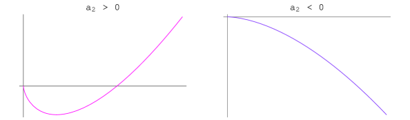
  FIG. 1.: $V(R)$ when $p<-6$.

• $-6<p<0$ (which implies $p_{1}<0<p_{2}$) (see fig. 2);

  

  FIG. 2.: $V(R)$ when $-6<p<0$.

• $p>0$ (which implies $p_{1}<p_{2}<0$) (see fig. 3).

  

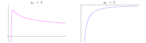
  FIG. 3.: $V(R)$ when $p>0$.

In the three cases corresponding to $a_{2}<0$, the evolution of the scale factor is monotonous because the potential is always negative, whereas for $a_{2}>0$, the potential vanishes at a nonzero value $R_{c}$ which represents the maximum value of the scale factor during the cosmological evolution. In the latter three subcases, cosmological expansion is thus followed by a collapse. This situation $a_{2}>0$ can be seen to be equivalent to the supergravity models with a bulk scalar field and an exponential superpotential [6]. It is also worth noticing that when $a_{2}<0$ the function $h(R)$ parametrizing the metric becomes negative. In that case the coordinate $R$ becomes time-like whereas $t$ becomes space-like and the Killing vector corresponding to translations of $t$ is then space-like. The brane normal vector is then given by $n_{a}=(\sqrt{A^{2}B^{2}}\dot{r},-\sqrt{B^{2}+B^{4}\dot{r}^{2}},0,0,0)$ which is a real quantity as soon as $\dot{r}^{2}$ is large enough. The rest of the analysis remains unchanged.

III Brane fluctuations

In this section, we turn to the analysis of the brane fluctuations allowed when the bulk geometry is left unperturbed. The fluctuations of the brane will be described by perturbing the embedding of the brane in the bulk spacetime, i.e. by writing

$$X^{A}(x^{\mu})=\bar{X}^{A}+\zeta\bar{n}^{A},$$ (52)

where the bar stands for the homogeneous quantities defined in the previous section. The four tangent vectors defined in (15) are then given by

$$e^{A}_{\mu}=\bar{e}^{A}_{\mu}+\delta e^{A}_{\mu}=\bar{e}^{A}_{\mu}+\partial_{\mu}\left(\zeta\bar{n}^{A}\right).$$ (53)

Substituting in the definition of the induced metric (16), and being careful to evaluate the (unchanged) bulk metric $g_{AB}$ at the perturbed brane location, one finds

$$h_{\mu\nu}=\bar{h}_{\mu\nu}+2\zeta\bar{K}_{\mu\nu}.$$ (54)

Using this expression, one can easily make the connection with the Bardeen potentials measuring the gauge invariant metric perturbations induced by the fluctuations of the brane position. In the longitudinal gauge, the perturbed metric reads

$$ds^{2}=-(1-2\Psi)dt^{2}+R^{2}(1+2\Phi)\delta_{ij}dx^{i}dx^{j},$$ (55)

and by comparing with (54), one finds that

$$\Psi=-\zeta\bar{K}^{\tau}_{\tau},\qquad\Phi={1\over 3}\zeta\bar{K}^{i}_{i}$$ (56)

which gives, after using the background junction conditions (27),

$$\Psi=-\frac{\kappa^{2}}{6}(2+3w)\rho\zeta$$ (57)

and

$$\Phi=-\frac{\kappa^{2}}{6}\rho\zeta$$ (58)

The metric perturbations are thus directly proportional to the brane fluctuation $\zeta$. We will return later to the evolution of the Bardeen potentials. The rest of this section is devoted to the derivation of the equation of motion that governs the evolution of the brane fluctuation. We first consider the perturbed junction conditions for the metric and then those for the scalar field.

A Perturbed junction conditions for the metric

As a first step, let us evaluate the perturbed normal vector, which can always be decomposed as

$$\delta n^{A}=\alpha\bar{n}^{A}+\beta^{\mu}\bar{e}^{A}_{\mu}.$$ (59)

The coefficients $\alpha$ and $\beta^{\mu}$ can be determined by perturbing the two equations in (18). They are given by

$$\alpha=-{1\over 2}\zeta\bar{n}^{A}\bar{n}^{B}\bar{n}^{C}\partial_{C}\bar{g}_{AB}$$ (60)

and

$${\bar{h}}_{\mu\nu}\beta^{\nu}=-\zeta\bar{n}^{A}\bar{e}^{B}_{\mu}\bar{n}^{C}\partial_{C}\bar{g}_{AB}-\bar{g}_{AB}\bar{n}^{A}\partial_{\mu}\left(\zeta\bar{n}^{B}\right).$$ (61)

Substituting the expressions (53) and (59) in the perturbation of the extrinsic curvature tensor (17), one obtains the expression

$$\delta K_{\mu\nu} = {1\over 2}\left[2\zeta\bar{n}^{C}\partial_{C}\bar{g}_{AB}\bar{e}^{A}_{(\mu}\bar{e}^{B}_{\nu)}+2\bar{g}_{AB}\left(\delta e^{A}_{(\mu}\partial_{\nu)}\bar{n}^{B}+\bar{e}^{A}_{(\mu}\partial_{\nu)}\delta n^{B}\right)+\right.$$ (64)

$$\left.+\left(\delta e^{A}_{\mu}\bar{e}^{B}_{\nu}\bar{n}^{C}+\bar{e}^{A}_{\mu}\delta e^{B}_{\nu}\bar{n}^{C}+\bar{e}^{A}_{\mu}\bar{e}^{B}_{\nu}\delta n^{C}\right)\partial_{C}\bar{g}_{AB}\right.$$

$$\left.+\zeta\bar{e}^{A}_{\mu}\bar{e}^{B}_{\nu}\bar{n}^{C}\bar{n}^{D}\partial_{C}\partial_{D}\bar{g}_{AB}\right].$$

The expression with an upper index and a lower index is also useful and can be obtained from the above expression by using the relation

$$\delta K_{\mu}^{\nu}=\bar{h}^{\nu\sigma}\delta K_{\sigma\mu}-2\zeta\bar{K}_{\mu\sigma}\bar{K}^{\sigma\nu},$$ (65)

where the indices for $\bar{K}^{\sigma\nu}$ are raised by using the inverse metric $\bar{h}^{\rho\sigma}$.

The explicit evaluation of the components of the perturbed brane extrinsic curvature tensor, for the metric (1), then yields

$$\delta K^{\tau}_{\tau} = \ddot{\zeta}-\left[{\left(B\ddot{r}+B^{\prime}\dot{r}^{2}\right)^{2}\over 1+B^{2}\dot{r}^{2}}+\left(1+B^{2}\dot{r}^{2}\right){{A^{\prime}}^{2}\over A^{2}B^{2}}+{A^{\prime}B^{\prime}\over AB^{3}}\right.$$ (67)

$$\left.+2{A^{\prime}B^{\prime}\over AB}\dot{r}^{2}-{A^{\prime\prime}\over AB^{2}}+2{A^{\prime}\over A}\ddot{r}\right]\zeta,$$

$$\delta K^{\tau}_{i} = \dot{\zeta}_{,i}-{R^{\prime}\over R}\dot{r}\zeta_{,i},$$ (68)

$$\delta K^{i}_{j} = \left[{R^{\prime}\over R}\dot{r}\dot{\zeta}+\left(-R^{\prime}B^{\prime}{1+B^{2}\dot{r}^{2}\over B^{3}R}-\dot{r}^{2}{A^{\prime}R^{\prime}\over AR}\right.\right.$$ (70)

$$\left.\left.-{R^{\prime}}^{2}{1+B^{2}\dot{r}^{2}\over B^{2}R^{2}}+R^{\prime\prime}{1+B^{2}\dot{r}^{2}\over B^{2}R}\right)\zeta\right]\delta^{i}_{j}-{\zeta_{,j}^{,i}\over R^{2}}$$

In the longitudinal gauge, which we shall use, the components of the perturbed brane energy momentum tensor read

$$\delta S^{\tau}_{\tau} = -\delta\rho,$$ (71)

$$\delta S^{\tau}_{i} = R(1+w)\rho\partial_{i}v,$$ (72)

$$\delta S^{i}_{j} = \delta P\delta^{i}_{j}+\delta\pi^{i}_{j},$$ (73)

where

$$\delta\pi^{i}_{j}=\delta\pi_{,j}^{,i}-{1\over 3}\delta^{i}_{j}\delta\pi_{,k}^{,k}$$ (74)

is the (traceless) anisotropic stress tensor, and the perturbed junction conditions for the metric, which follow from (27), are given by

$$\delta K^{\mu}_{\nu}=-{\kappa^{2}\over 2}\left(\delta S^{\mu}_{\nu}-{\delta S\over 3}\delta^{\mu}_{\nu}\right).$$ (75)

Inserting (71-73), this gives explicitly

$$\delta K^{\tau}_{\tau} = {\kappa^{2}\over 6}\left(2\delta\rho+3\delta P\right),$$ (76)

$$\delta K^{\tau}_{i} = -{\kappa^{2}\over 2}R(1+w)\rho\partial_{i}v,$$ (77)

$$\delta K^{i}_{j} = -{\kappa^{2}\over 2}\left({1\over 3}\delta\rho\delta^{i}_{j}+\delta\pi^{i}_{j}\right).$$ (78)

The second equation (68) determines, once $\zeta$ is known, the velocity potential $v$, except when the equation of state is $w=-1$, in which case one gets the constraint

$$\dot{\zeta}={R^{\prime}\over R}\dot{r}\zeta\qquad(w=-1).$$ (79)

This implies that the perturbation reads

$$\zeta=R(\tau)C(k)$$ (80)

up to a global translation of the brane. The function $C(k)$ will be determined later.

Finally, equation (78) can be decomposed into a trace and a traceless part, giving respectively

$${R^{\prime}\over R}\dot{r}\dot{\zeta}+\left(-R^{\prime}B^{\prime}{1+B^{2}\dot{r}^{2}\over B^{3}R}-\dot{r}^{2}{A^{\prime}R^{\prime}\over AR}-{R^{\prime}}^{2}{1+B^{2}\dot{r}^{2}\over B^{2}R^{2}}\right.$$ (81)

$$\left.+R^{\prime\prime}{1+B^{2}\dot{r}^{2}\over B^{2}R}\right)\zeta-{1\over 3R^{2}}\Delta\zeta=-{\kappa^{2}\over 6}\delta\rho$$ (82)

and

$${1\over R^{2}}\left(\zeta_{,j}^{,i}-{1\over 3}\Delta\zeta\delta^{i}_{j}\right)={\kappa^{2}\over 2}\delta\pi^{i}_{j}.$$ (83)

The last equation simply gives

$$\delta\pi=\frac{2}{\kappa^{2}}\frac{\zeta}{R^{2}}$$ (84)

and shows that the anisotropic stress is intrinsically related to the brane fluctuation.

B Perturbed junction condition for the scalar field

The next step in order to establish the equations of motion for the brane fluctuations is to write down the perturbed junction condition for the scalar field. The first order perturbation of (37) yields

$$\left[\delta n^{A}\partial_{A}\phi+\zeta n^{A}n^{B}\partial_{A}\partial_{B}\phi\right]=-\kappa^{2}\,\xi^{\prime}\,\delta S-\kappa^{2}S\,\xi^{\prime\prime}(n^{A}\partial_{A}\phi)\zeta.$$ (85)

Taking into account $Z_{2}$ symmetry and using the background junction condition (38), its derivative along the trajectory, and the other junction condition (29), one finds, after some algebra, that eq. (85) takes the form

$$\left(3w-1\right)\left\{{R^{\prime}\over R}\dot{r}\dot{\zeta}+\left[{\hat{\rho}}^{2}\left({RR^{\prime\prime}\over{R^{\prime}}^{2}}-1\right)-{R^{\prime}\over R}\left({B^{\prime}\over B^{3}}+\left({A^{\prime}\over A}+{B^{\prime}\over B}\right)\dot{r}^{2}\right)\right]\zeta\right\}$$ (86)

$$+3{\hat{\rho}}^{2}{R\over R^{\prime}}{\dot{w}\over\dot{r}}\zeta={\kappa^{2}\over 6}\left(1-3c_{p}^{2}\right)\delta\rho$$ (87)

where we have introduced

$$c_{p}^{2}=\frac{\delta p}{\delta\rho}$$ (88)

Combining (87), (82) and (76), one sees that the matter perturbation can be eliminated to give a differential equation that depends only on $\zeta$. It has the form of a wave equation. and reads

$$\ddot{\zeta}+(2+3w){\dot{R}\over R}\dot{\zeta}-{\Delta\zeta\over R^{2}}+\left\{{A^{\prime\prime}\over AB^{2}}-{A^{\prime}B^{\prime}\over AB^{3}}-(2+3w){A^{\prime}R^{\prime}\over AR}\dot{r}^{2}\right.$$ (89)

$$\left.+(2+3w){\hat{\rho}}^{2}\left[-(2+3w)-{B^{\prime}R^{\prime}\over BR}+{RR^{\prime\prime}\over{R^{\prime}}^{2}}-1\right]\right\}\zeta=0.$$ (90)

Introducing the function $\psi$ defined by

$$\psi=R^{(1+3w)/2}\zeta$$ (91)

and using the conformal time $\eta$ defined by $d\tau=Rd\eta$, one can rewrite the wave equation in the simple form

$${d^{2}\psi\over d\eta^{2}}+(k^{2}+{\cal M}^{2})\psi=0,$$ (92)

where the effective mass is given by

$${\cal M}^{2} = R^{2}\left[-\frac{1+3w}{2}\left(\frac{\ddot{R}}{R}+\frac{1+3w}{2}\frac{\dot{R}^{2}}{R^{2}}\right)+\frac{A^{\prime\prime}}{AB^{2}}-\frac{A^{\prime}B^{\prime}}{AB^{3}}-(2+3w)\frac{A^{\prime}R^{\prime}}{AR}\dot{r}^{2}\right.$$ (94)

$$\left.+(2+3w){\hat{\rho}}^{2}\left(\frac{RR^{\prime\prime}}{R^{\prime 2}}-\frac{B^{\prime}R}{BR^{\prime}}-3(1+w)\right)\right].$$

We have thus obtained the wave equation governing the intrinsic brane fluctuations in the general case. Initially, we started from a system of five equations, (76), (77), (87), (84) and (82), all obtained from the junction conditions, either of the metric or of the scalar field. These five equations contain one dynamical equation, which has been expressed above in terms of the quantity $\zeta$ (or $\psi$) and four constraints which yield respectively the energy density $\delta\rho$, the pressure $\delta P$, the four-velocity potential $v$ and the anisotropic stress $\delta\pi$. In contrast with the standard cosmological context where one can choose beforehand the relation between $\delta P$ and $\delta\rho$, and the anisotropic stress, they are here completely determined by the constraints once a solution for $\zeta$ is given. This is necessary to get a configuration where the brane is fluctuating while the background is unaffected. Intuitively, this means that the gravitational effect due to the geometrical fluctuations of the brane must be exactly compensated the distribution of matter in the brane, so that the net gravitational effect due to the presence of the brane is completely cancelled in the bulk.

In the rest of the paper, we will specialize our study to specific solutions, which will simplify the expression of the effective mass.

IV Perturbations in Dilatonic Backgrounds

In this section we will focus on the dilatonic backgrounds described earlier, corresponding to exact solutions for an exponential potential. Using the previous general result about the mass term ${\cal M}^{2}$ in the wave equation, we can now specialize these results to the dilatonic backgrounds. We will concentrate on the case where the background equation of state parameter $w$ is constant. Substituting the solution (10) in the expression (94), one finds that the square mass reads

$${\cal M}^{2} = \frac{R^{2}}{4}\left\{(1+w)\left[{2V_{0}\over 3\alpha^{2}-4}(5+3w-6\alpha^{2})R^{-6\alpha^{2}}-3(7+9w+6\alpha^{2})\hat{\rho}^{2}\right]\right.$$ (96)

$$\left.+3(1-w)(3\alpha^{2}-1+3w){\cal C}R^{-4-3\alpha^{2}}\right\}$$

where

$$\hat{\rho}^{2}=\frac{1+B^{2}\dot{r}^{2}}{B^{2}}(\frac{R^{\prime}}{R})^{2}$$ (97)

Notice that for $w=-1$ only the ${\cal C}$ dependent term remains. Using the decomposition $\zeta=C(k)R$ we find that

$$(k^{2}+{\cal M}^{2})C(k)=0$$ (98)

which leads to $C(k)=0$ and therefore the absence of brane fluctuations for $w=-1$.

In the following we will concentrate on the ${\cal C}=0$ case. Introducing the parameter $p$ defined in (50), the squared mass is now given by

$${\cal M}^{2} = {3\over 4}(1+w)^{2}\left[-a_{1}(9+p)R^{p_{1}}+a_{2}(3-p)R^{p_{2}}\right]$$ (99)

$$= (1+w)^{2}\frac{V_{0}}{2(3\alpha^{2}-4)}\left[{(3-p)\over R^{p(1+w)}}-\delta{(9+p)\over R^{(6+p)(1+w)}}\right],$$ (100)

with

$$\delta=\frac{3(3\alpha^{2}-4)}{2V_{0}}\hat{\rho}_{1}^{2}.$$ (101)

We will now treat separately the cases of positive or negative $a_{2}$, i.e. of $\delta$, which correspond to very different behaviours.

A Bouncing branes

Let us concentrate first on the case

$$a_{2}\equiv\frac{2V_{0}/3}{3\alpha^{2}-4}=\gamma^{2}>0,$$ (102)

where $\gamma$ has the dimension of mass.

The motion can be conveniently analysed by defining $y=R^{6(w+1)}$. The equation of motion (46) yields

$${dy\over 6(1+w)\sqrt{\delta-y}}y^{-\frac{1}{2}+\frac{p}{12}}=\pm\gamma d\eta$$ (103)

Let us define $n$ as

$$n=\frac{p-6}{12}$$ (104)

The scale factor is then given by the implicit relation

$${y^{1+n}\over 1+n}{\mathcal{F}}(1+n,{1\over 2},2+n,{y\over\delta})=\pm 6\gamma(1+w)\sqrt{\delta}\,\eta+\eta_{0}$$ (105)

${\mathcal{F}}$ being the hypergeometric function. Of course the scale factor is only determined after inverting these equations. The motion is bounded from above by $y=\delta$. For a brane whose scale factor increases initially, it reaches a maximal value corresponding to $\delta$ before bouncing back and being irredeemingly attracted by the singularity located at $R=0$. It is interesting to notice that for $p\leq-6$ the singularity is reached at infinite conformal time while for $p>-6$ it takes a finite amount of conformal time to the brane in order to reach the singularity.

Let us now analyse the square mass driving the brane fluctuations. We have plotted the different cases in Figure 4. There is a qualitative change of behaviour for the square mass when $p>-6$. Below the critical value $p=-6$ the mass vanishes at the singularity when $R$ vanishes. This leads to an oscillatory behaviour of the brane fluctuation. Above that threshold the squared mass becomes infinitely negative at the singularity leading to an instability of the brane to fluctuations, i.e. the brane tends to be ripped to shreds by the presence of the singularity.

FIG. 4.: ${\mathcal{M}}^{2}$ in a bouncing universe. In the left picture ($p\leq-6$), the red line corresponds to $p\leq-9$, the green line represents $-9<p<-6$ and the blue line displays the critical value $p=-6$. The right picture shows ${\mathcal{M}}^{2}$ for $p>-6$ : the red line corresponds to $-6<p<0$, the green line to $p=0$, the blue line stands for $0<p<3$ whereas the yellow line stands for $p\geq 3$.

In the cases $-9<p<-6$, the square mass is negative for small values of $R$, reaches a minimum and then increases up to positive values with increasing $R$. However, values of $R$ greater than $\delta^{1/(6(w+1))}$ are irrelevant since the background evolution bounces when reaching this maximum value. The position of the minimum is given by

$$y_{m}={(6+p)(9+p)\over p(3-p)}\delta<\delta,$$ (106)

whereas the scale factor corresponding to ${\cal M}^{2}=0$ is given by

$$y_{0}={(9+p)\over(3-p)}\delta.$$ (107)

For $-6<p<3$, the square mass starts from negative values and becomes positive after the critical value $y_{0}$ which is less than $\delta$ only for $p<-3$. In other words, for cases $p>-3$, the region corresponding to positive square mass is irrelevant.

We can recover this qualitative analysis by studying the solutions of the wave equation (92), which, in terms of the variable $y$, reads

$${d^{2}\psi\over dy^{2}}\left(\delta-y\right)+{d\psi\over dy}\left(n-{1\over 2}-{n\delta\over y}\right)+y^{2n}\tilde{k}^{2}\psi={y\left(4n+1\right)+\delta\left(4n+5\right)\over{16y^{2}}}\psi$$ (108)

with

$$\tilde{k}^{2}={k^{2}\over 36\gamma^{2}\left(1+w\right)^{2}}$$ (109)

The variable $y$ evolves between $0<y<\delta$.

The asymptotical behaviour of the perturbation near the singularity $y=0$ depends on $n$ :

$$\psi\sim\left\{\begin{array}[]{ll}{\mathcal{C}}_{1}y^{-{1\over 4}}+{\mathcal{C}}_{2}y^{n+{5\over 4}},&\;n>-1\\ {\mathcal{C}}_{1}\cos\left(\sqrt{{\frac{\tilde{k}^{2}}{\delta}-\frac{1}{16}}}\ln\,y\right)+{\mathcal{C}}_{2}\sin\left(\sqrt{{\frac{\tilde{k}^{2}}{\delta}-\frac{1}{16}}}\ln\,y\right),&\;n=-1\\ {\mathcal{C}}_{1}\cos\left(y^{n+1}+\alpha\right)+{\mathcal{C}}_{2}\sin\left(y^{n+1}+\alpha\right),&\;n<-1\end{array}\right.$$ (113)

Notice that for $p<-6$ the brane oscillates for an infinite amount of conformal time before reaching the singularity. For $p>-6$, the brane stops oscillating and hits the singularity in a finite amount of conformal time. For $p=-6$ the brane oscillates only for small length-scales corresponding to $\tilde{k}>4\sqrt{\delta}$.

The Bardeen potentials, given in (57) and (58), are also worth investigating. They are proportional,

$$\Psi=(2+3w)\Phi,$$ (114)

and related to the brane fluctuation according to

$$\Phi\propto R^{{(9+p)\over 2(1+w)}}\psi.$$ (115)

One thus notices the critical value $p=-9$, above which the Bardeen potentials are enhanced, for an expanding universe, with respect to $\psi$. One can compute numerically the evolution of the perturbation, the Bardeen potential and the scale factor as a function of the conformal time (see Figure 5).

FIG. 5.: Perturbation (red line), Bardeen potential (blue line) and scale factor (green line) during the contracting phase of a bouncing universe, as functions of the conformal time.

B Ever expanding branes

We now turn to the case

$$a_{2}\equiv\frac{2V_{0}/3}{3\alpha^{2}-4}=-\gamma^{2}<0,$$ (116)

Using once more the $y$ variable we can rewrite the background evolution equation as

$${dy\over 6(1+w)\sqrt{y+|\delta|}}y^{-\frac{1}{2}+\frac{p}{12}}=\pm\gamma d\eta.$$ (117)

FIG. 6.: ${\mathcal{M}}^{2}$ in an inflationary universe. The picture $p\leq-6$ depicts three different cases : $p<-9$ (red line), $-9\leq p<-6$ (green line) and $p=-6$ (blue line). In the second picture, where $-6<p\leq-3$, the red and blue lines illustrate $-6<p<0$, the green line stands for $p=0$ and the yellow line stands for $0<p\leq 3$. The third picture represents $p>3$.

Since $p_{2}>p_{1}$, the asymptotic behaviour at early times, i.e. at small $R$, is dominated, both for the background and for the perturbations, by the $R^{p_{1}}$ term (since $p_{2}>p_{1}$), which does not depend on the sign of $a_{2}$. Therefore, the asymptotic behaviour at early times for ever expanding branes is exactly the same as that found in the case of bouncing branes.

For large $R$, conversely, the dominating term is $R^{p_{2}}$. For the background, this leads to a power-law behaviour of the scale factor, explicitly given by

$$R(\eta)\simeq\left[{p\over 2}(1+w)\gamma\eta\right]^{2\over p(1+w)},$$ (118)

which, in terms of the cosmic time, translates into

$$R(\tau)\propto\tau^{2/\left(p(1+w)+2\right)}.$$ (119)

As soon as $p<0$, one gets an accelerated expansion, similar to the standard four-dimensional power-law inflation, which can be obtained from a scalar field with an exponential potential. For $p>0$, one gets a decelerated power-law expansion. It is instructive to compare the power-law expansion for the brane with the standard expansion law, which is given by

$$R(\tau)\propto\tau^{2/3(1+w)}.$$ (120)

Substituting the expression (118) in the squared mass, one finds

$${\cal M}^{2}=-{3(3-p)\over p^{2}}{1\over\eta^{2}}.$$ (121)

Note that, in the case of power-law inflation, one can derive a second-order differential equation of the form (92) for a canonical variable which is a linear combination of the scalar field perturbation and of the (scalar) metric perturbation. For a power-law $a\sim t^{q}$, one would find

$${\cal M}^{2}_{eff}=-{q(2q-1)\over(q-1)^{2}}{1\over\eta^{2}}.$$ (122)

It is easy to check that our expression for ${\cal M}^{2}$ does not coincide with the ${\cal M}^{2}_{eff}$ deduced from power-law inflation, for the same evolution of the background. With power-law inflation, the spectrum for the Bardeen potential(s) is given by

$${\cal P}\sim k^{-2/(q-1)},$$ (123)

which tends to a scale-invariant spectrum for large power $q$.

In our case, we obtain that the fluctuations are

$$\psi=\sqrt{-\eta}\left[\alpha_{1}H^{(1)}_{\nu}(-k\eta)+\alpha_{2}H^{(2)}_{\nu}(-k\eta)\right]$$ (124)

where

$$\nu=\frac{p-6}{2p}$$ (125)

If one assumes that $\psi$ is given in the asymptotic past $\eta\rightarrow-\infty$ as the usual vacuum solution in inflation, i.e.

$$\psi\sim{1\over\sqrt{k}}e^{-ik\eta},\qquad k|\eta|\gg 1,$$ (126)

then this means that $\alpha_{2}=0$ and the behaviour on long wavelengths is given by

$$\psi\sim(-\eta)^{{1\over 2}-\nu}k^{-\nu}\sim R^{{3\over 2}(1+w)}k^{-\nu},\qquad k|\eta|\ll 1.$$ (127)

Using the relation between $\psi$ and the Bardeen potential, one thus finds that the spectrum for $\Phi$ is given by

$${\cal P}_{\Phi}\sim R^{9+p+3(1+w)^{2}\over 1+w}k^{-2\nu}.$$ (128)

Contrary to the four dimensional inflationary case, the spectrum of the Bardeen potential is not constant outside the horizon. Moreover the spectrum is red and far from being scale-invariant. Hence, despite an inflationary phase on the brane, the intrinsic fluctuations of a brane in a dilatonic background are not a candidate for the generation of primordial fluctuations.

FIG. 7.: Left picture : Perturbation as a function of $k\eta$. For $p<0$, the perturbation always diverges near the singularity. Right picture : perturbation (red line), Bardeen potential (blue line) and scale factor (green line ) for $p>0$.

V Conclusion

We have investigated the fluctuations of a moving brane in a dilatonic background. These fluctuations are represented by a scalar mode on the brane corresponding to ripples along the normal direction to the brane. As the brane fluctuates, it induces metric fluctuations, in particular we have found that the induced metric appears naturally in the longitudinal gauge with two unequal Bardeen potentials $\Phi$ and $\Psi$. The fact that these potentials are not equal springs from the presence of anisotropic stress on the brane. For a fixed equation of state for the matter content on the brane, for instance cold dark matter, we find that the two Bardeen potentials are proportional. As such this implies that a single gauge invariant observable $\Phi$ characterizes the brane fluctuations.

Our approach differs from the projective approach [4, 5] in as much as we have not considered the perturbed Einstein equations on the brane. This allows us to free ourselves from the thorny problem of the projected Weyl tensor on the brane.

We have focused on the motion and fluctuations of branes in a particular class of dilatonic backgrounds. These backgrounds correspond to an exponential potential and an exponential coupling of the bulk scalar field to the brane. The motion of the brane is either of the bouncing type or the ever-expanding form. In the bouncing case we find that the brane cannot escape towards infinity, it is bound to a singularity which is either null or time-like. In the time-like case, i.e. when it appears at a finite distance in conformal coordinates, the fluctuations of the brane are unbounded implying that the brane is ripped by the strong gravity around the singularity. In the null case, i.e. when the singularity is at conformal infinity, the fluctuations oscillate in a bounded manner while converging to the singularity. The bouncing case is equivalent to the behaviour of a brane in a supergravity background. As we only consider intrinsic fluctuations of the brane in an unperturbed bulk, this corresponds to a situation where supersymmetry is preserved by the bulk while broken by the brane motion. Therefore the bouncing brane fluctuations correspond to fluctuations of a non-BPS brane embedded in a supergravity background.

In the ever-expanding scenario, we can distinguish two possibilities. The brane can escape to infinity with a scale factor which is either expanding in a decelerating manner or accelerating, i.e. corresponding to an inflationary era of the power law type. In the decelerating case, the brane eventually oscillates forever. In the inflationary case, the brane is such that any fluctuation of a giving length scales oscillates until it freezes in while passing through the horizon. Of course this scenario is reminiscent of four-dimensional inflation modelled with a scalar field. Here the features of inflation, i.e. the relationship between the power spectrum and the scale factor, differ from the four dimensional case. This is an interesting observation as it leads to a new twist in the building of inflationary models. One might hope that alternative scenarios to four-dimensional inflation may emerge from five dimensional brane models and their fluctuations.

REFERENCES

- [1] D. Langlois, arXiv:hep-th/0209261.
- [2] A. Lukas, B. A. Ovrut, K. S. Stelle and D. Waldram Phys. Rev. D 59, 086001 (1999) [arXiv:hep-th/9803235]; Nucl. Phys. B 552, 246 (1999) [arXiv:hep-th/9806051]; A. Lukas, B. A. Ovrut and D. Waldram, Phys. Rev. D 60, 086001 (1999) [arXiv:hep-th/9806022]; Phys. Rev. D 61, 023506 (2000) [arXiv:hep-th/9902071].
- [3] H. A. Chamblin and H. S. Reall, Nucl. Phys. B 562, 133 (1999) [arXiv:hep-th/9903225].
- [4] K. i. Maeda and D. Wands, Phys. Rev. D 62, 124009 (2000) [arXiv:hep-th/0008188].
- [5] A. Mennim and R. A. Battye, Class. Quant. Grav. 18, 2171 (2001) [arXiv:hep-th/0008192].
- [6] P. Brax and A. C. Davis, Phys. Lett. B 497, 289 (2001) [arXiv:hep-th/0011045]; P. Brax, C. van de Bruck and A. C. Davis, JHEP 0110, 026 (2001) [arXiv:hep-th/0108215].
- [7] A. Feinstein, K. E. Kunze and M. A. Vázquez-Mozo, Phys. Rev. D 64, 084015 (2001) [arXiv:hep-th/0105182]; K. E. Kunze and M. A. Vázquez-Mozo, Phys. Rev. D 65, 044002 (2002) [arXiv:hep-th/0109038].
- [8] O. De Wolfe, D. Z. Freedman, S. Gubser and A. Karch Phys. Rev. D 62 (2000) 0460008 [arXiv: hep-th/9909134]
- [9] C. Csaki, J. Erlich, C. Grojean and T. Hollowood Nucl. Phys. B 584 (2000) 359 [arXiv: hep-th/ 0004133]
- [10] J. E. Lidsey, Phys. Rev. D 64, 063507 (2001) [arXiv:hep-th/0106081].
- [11] C. Grojean, F. Quevedo, G. Tasinato and I. Zavala C., JHEP 0108, 005 (2001) [arXiv:hep-th/0106120].
- [12] D. Langlois and M. Rodríguez-Martínez, Phys. Rev. D 64, 123507 (2001) [arXiv:hep-th/0106245].
- [13] S. C. Davis, JHEP 0203, 054 (2002) [arXiv:hep-th/0106271]; JHEP 0203, 058 (2002) [arXiv:hep-ph/0111351].
- [14] C. Charmousis, Class. Quant. Grav. 19, 83 (2002) [arXiv:hep-th/0107126].
- [15] E. E. Flanagan, S. H. Tye and I. Wasserman, Phys. Lett. B 522, 155 (2001) [arXiv:hep-th/0110070].
- [16] W. D. Goldberger and M. B. Wise, Phys. Rev. Lett. 83 (1999) 4922 [arXiv: hep-th/9907447], Phys. Rev. D 60 (1999) 107505 [arXiv: hep-th 9907218]
- [17] J. Garriga and A. Vilenkin, Phys. Rev. D 44 (1991) 1007
- [18] J. Guven, Phys. Rev. D48 (1993) 4604
- [19] A. Ishibashi and T. Tanaka, [arXiv: gr-qc/ 0208006]
- [20] T. Boehm and D. A. Steer, Phys. Rev. D 66 (2002) 063510 [arXiv:hep-th/0206147].
- [21] R. G. Cai, J. Y. Ji and K. S. Soh, Phys. Rev. D 57, 6547 (1998) [arXiv:gr-qc/9708063].
- [22] N. Deruelle, T. Dolezel and J. Katz, Phys. Rev. D 63, 083513 (2001) [arXiv:hep-th/0010215].