Trans-Planckian Dark Energy?

Abstract

It has recently been proposed in Refs. MBK01 ; BFM02 ; BM02 that the dark energy could be attributed to the cosmological properties of a scalar field with a non-standard dispersion relation that decreases exponentially at wave-numbers larger than Planck scale ($k_{\rm phys}>M_{\rm Pl}$). In this scenario, the energy density stored in the modes of trans-Planckian wave-numbers but sub-Hubble frequencies produced by amplification of the vacuum quantum fluctuations would account naturally for the dark energy. The present article examines this model in detail and shows step by step that it does not work. In particular, we show that this model cannot make definite predictions since there is no well-defined vacuum state in the region of wave-numbers considered, hence the initial data cannot be specified unambiguously. We also show that for most choices of initial data this scenario implies the production of a large amount of energy density (of order $\sim M_{\rm Pl}^{4}$) for modes with momenta $\sim M_{{\rm Pl}}$, far in excess of the background energy density. We evaluate the amount of fine-tuning in the initial data necessary to avoid this back-reaction problem and find it is of order $H/M_{{\rm Pl}}$. We also argue that the equation of state of the trans-Planckian modes is not vacuum-like. Therefore this model does not provide a suitable explanation for the dark energy.

I Introduction

Recently, it has been claimed in a series of articles MBK01 ; BFM02 ; BM02 that the cosmic dark energy component could be explained naturally by the trans-Planckian energy of a scalar field with a suitable non-linear dispersion relation in the trans-Planckian regime. Such dispersion relations, which relate the frequency $\omega_{\rm phys}$ to the wave-number $k_{\rm phys}$ of a scalar field wave-packet, and which depart from the standard linear dispersion relation in the trans-Planckian regime are a way of modeling phenomenologically the unknown physics for sub-Planckian wavelengths. They have been used extensively in the recent literature in the context of black-hole physics U95 and of the inflationary trans-Planckian problem MB .

In the particular case considered in Refs. MBK01 ; BFM02 ; BM02 , the dispersion relation departs from its standard linear form and approach a decreasing exponential at large wave-numbers. This type of dispersion relation could possibly emerge from string theory BFM02 . It has been argued that the energy density of the modes of sub-Planckian wavelengths and sub-Hubble frequencies (referred to as “tail” modes) is naturally of the same order as the critical energy density today and has the same equation of state as a cosmological constant. Hence, it could account without fine-tuning for the dark energy. The energy density contained in the tail today has been calculated in Ref. MBK01 by solving for the time evolution of a test quantum scalar field evolving in the curved cosmological background, assuming its initial state at the onset of inflation is the vacuum. The equation of state of the tail modes has been calculated in Ref. BM02 and its cosmological evolution has been solved to argue that the cosmic coincidence problem (why does the dark energy dominate now?) is solved.

In this paper we argue that this model does not and can not work for several reasons. We first argue that the energy density and equation of state of the “tail” modes depend directly on the choice of initial data for the scalar field, and that this latter cannot be specified unambiguously since there is no preferred initial vacuum state (Section II). This implies that any cosmological consequence derived depends directly on the ad-hoc choice of initial data (initial quantum state). We then show that the violation of the Wentzel-Kramers-Brillouin (WKB) approximation in the remote past for all co-moving wave-numbers, which is inevitable in the present scenario, implies the continuous production at all times of a large amount of quanta with physical wave-number $\sim M_{{\rm Pl}}$ (Section III). This finding is in agreement with general arguments given by Starobinsky S01 (this latter work did not however study the present scenario). We evaluate the amount of energy density produced for modes of physical wave-number and frequency $\sim M_{{\rm Pl}}$ for various choices of initial data and conclude that it is generically of order $M_{{\rm Pl}}^{4}$. This process takes place at all times, and since the energy density produced is much larger than the background energy density, it implies that the semi-classical perturbative framework on which the model of Refs. MBK01 ; BFM02 ; BM02 rests breaks down. In an earlier study, devoted to constructing an effective stress-energy tensor for theories with non-linear dispersion relations LMMU01 , we already criticized this model by arguing that it led generically to the wrong equation of state. We revisit this issue further in Section IV, where we prove that the effective energy-momentum tensor we derived earlier is well-behaved, thus disproving an improper claim of Ref. BM02 and confirming our earlier criticisms. We provide a summary of our conclusions in Section V.

II Initial conditions for the mode evolution

Refs. MBK01 ; BFM02 ; BM02 consider a scalar field, $\phi$, with a non-linear dispersion relation that is linear in the sub-Planckian regime and approaches a decreasing exponential at trans-Planckian wave-numbers (i.e. for $k_{\rm phys}\gtrsim k_{\rm c}$, $k_{\rm c}\sim M_{{\rm Pl}}$ being a fundamental characteristic scale). This dispersion relation is shown in Fig. 1. This scalar field is assumed to describe the density (scalar) perturbations and/or the primordial gravitational waves. The “tail” modes are thus interpreted as a bath of gravitons of super-Planckian wavelengths and sub-Hubble frequencies. This scalar field is treated as a test-field (its back-reaction on the background is neglected) and is quantized on the curved cosmological background. Assuming that the “tail” modes of this field are initially in a well chosen vacuum state as $\eta\rightarrow-\infty$ ($\eta$ denoting conformal time), the occupation number at late times ($\eta\rightarrow+\infty$) of quanta extracted out of the vacuum by the dynamical background has been calculated in Ref. MBK01 . This occupation number can then be used to calculate the energy density stored today in the “tail”. This is the thread of the calculation performed in Ref. MBK01 , which we now follow in some detail. This discussion will take us to the two main arguments that we bring forward against this model (given in this Section and the following).

Figure 1: Dispersion relation $\omega_{\rm phys}$ vs $k_{\rm phys}$. Region I (hashed area) corresponds to the “tail” modes for which $\omega_{\rm phys}\leq H$ [and $k_{\rm phys}\geq K(\eta)$]. Region II corresponds to the sub-horizon modes ($k_{\rm phys}\geq H$) that are outside of the tail, while region III corresponds to the super-horizon modes $k_{\rm phys}\leq H$. The fundamental scale $k_{\rm c}$ is also indicated.

The equation of motion of a scalar field $\phi\equiv\mu/a$ in a Friedmann-Lemaître-Robertson-Walker (FLRW) space-time with scale factor $a(\eta)$ reads:

$$\mu_{k}^{\prime\prime}+\left[\omega^{2}-(1-6\xi)\frac{a^{\prime\prime}}{a}\right]\mu_{k}=0,$$ (1)

where $\xi$ is a coupling parameter to gravity and a prime denotes differentiation with respect to conformal time. $k=ak_{\rm phys}$ is the co-moving wave-number and $\omega=a\omega_{\rm phys}$ is the co-moving frequency. $\xi=0$ for tensor perturbations degrees of freedom and $\xi=1/6$ for a conformally coupled field. The scale factor is taken to be a power law in conformal time, $a=|\eta/\eta_{\rm c}|^{-\beta}$, and the following dispersion relation, parameterized by two parameters $\epsilon_{1}$ and $\epsilon_{3}$ with $\epsilon_{3}=4-2\epsilon_{1}$ in order to insure that the dispersion relation is linear for small wave-numbers, is introduced:

$$\omega_{\rm phys}^{2}(k_{\rm phys})=k_{\rm phys}^{2}\left[\frac{\epsilon_{1}}{1+{\rm e}^{x}}+\frac{\epsilon_{3}{\rm e}^{x}}{(1+{\rm e}^{x})^{2}}\right],$$ (2)

with $x\equiv(k_{\rm phys}/k_{\rm c})^{1/\beta}=A|\eta|$ with $A\equiv(k/k_{\rm c})^{1/\beta}/|\eta_{\rm c}|$. A problem with this dispersion relation is that it depends on the power-law index $\beta$ of the scale factor. If taken literally, this means that the dispersion relation, or the physical frequency of a given mode, changes as the scale factor power-law index $\beta$ changes between various cosmological eras (e.g. inflation / radiation domination / matter domination). More importantly one easily sees that the above dispersion relation has a pathological behavior in the radiation ($\beta=-1$) or matter ($\beta=-2$) dominated eras. In fact, for $\beta<0$, it implies $\omega_{\rm phys}/k_{\rm phys}\rightarrow 0$ as $k_{\rm phys}\rightarrow 0$, whereas one should instead reach the linear dispersion relation in that regime with $\omega_{\rm phys}/k_{\rm phys}\rightarrow 1$. Since Ref. MBK01 focused on the case of de Sitter space-time with $\beta=1$, we set $\beta=1$ in the above dispersion relation, i.e., the above $x$ should be understood as $x\equiv k_{\rm phys}/k_{\rm c}$. This reformulated dispersion relation thus coincides with that used in Ref. MBK01 for de Sitter space. However, in the matter dominated era, for instance, we have $x=k_{\rm phys}/k_{\rm c}\propto\eta^{-2}$ and the general class of solutions to the field equation obtained in Ref. MBK01 does not hold anymore. The linear dependence of $x$ on $\eta$ is lost for background metrics other than de Sitter, but the linear dependence of $\omega_{\rm phys}$ on $k_{\rm phys}$ is preserved in the small $k_{\rm phys}$ limit for all metrics, which is obviously an imperative. The field equation can finally be rewritten as:

$$\mu_{k}^{\prime\prime}+\biggl{\{}k^{2}\biggl{[}\frac{\epsilon_{1}}{1+{\rm e}^{x}}+\frac{\epsilon_{3}{\rm e}^{x}}{(1+{\rm e}^{x})^{2}}\biggr{]}-(1-6\xi)\frac{\beta(\beta+1)}{\eta^{2}}\biggr{\}}\mu_{k}=0\,,$$ (3)

with, again, $x(\eta)\equiv k_{\rm phys}/k_{\rm c}=k/[a(\eta)k_{\rm c}]$. The solution to this equation depends on the value of $\xi$ and $\beta$. In Ref. MBK01 , the contribution of the $[a^{\prime\prime}/a]$ term is assumed to be negligible at early times. However the above equation shows that this is not the case; denoting by $\Omega_{k}^{2}$ the term in curly brackets in Eq. (3), one has $\Omega_{k}^{2}\simeq k^{2}(\epsilon_{1}+\epsilon_{3}){\rm e}^{-k|\eta|^{\beta}/(k_{\rm c}|\eta_{\rm c}|^{\beta})}-\beta(\beta+1)(1-6\xi)/\eta^{2}$ as $\eta\rightarrow-\infty$ and the term $a^{\prime\prime}/a\propto\eta^{-2}$ is always dominant in that limit if $\xi\neq 1/6$ ($\beta\geq 1$, $\eta\rightarrow-\infty$). Therefore, in the limit $\xi\neq 1/6$ and $\eta\rightarrow-\infty$ the two independent solutions to the field equation are power-laws in $\eta$:

$$\mu_{k}\propto\left(\frac{\eta}{\eta_{\rm c}}\right)^{\alpha{{}_{\pm}}},\quad\alpha_{\pm}=\frac{1}{2}\pm\sqrt{\frac{1}{4}+\beta(1+\beta)(1-6\xi)}\,.$$ (4)

This is an important point as it implies that the mode function does not behave as a plane wave in the limit $\eta\rightarrow-\infty$ when $\xi\neq 1/6$. The solution to the field equation in this limit is reminiscent of the mode freezing in inflationary theories for fields with linear dispersion relations and $\xi=0$ when the mode exits the horizon.

It is also argued that the term in $a^{\prime\prime}/a$ can be absorbed at late times in a redefinition of the dispersion relation. However this cannot be correct since by construction, the dispersion relation $\omega_{\rm phys}(k_{\rm phys})$ depends only on $k_{\rm phys}$, i.e. time only enters via $k_{\rm phys}$. Therefore, one can absorb a term $a^{\prime\prime}/a\propto\eta^{-2}$ into $\omega_{\rm phys}^{2}/a^{2}$ only if $\beta=1$ (de Sitter space-time), as inspection of Eq. (3) reveals. In effect, the curly bracket of Eq. (3) can then be rewritten as $a^{-2}$ times a function of $k\eta\propto k_{\rm phys}$. But, in that particular case, the redefined modified dispersion relation does not have an exponential shape anymore, since $\omega_{\rm phys}$ approaches a constant ($\sim H$) as $k_{\rm phys}\rightarrow+\infty$. However, this should not give the impression that the corresponding solution is a plane wave since, evidently, the co-moving frequency $\omega$ which enters Eq. (1) still behaves as $\propto\eta^{-2}$. Moreover in the case of a matter or radiation dominated cosmology, one cannot absorb the scale factor term in the dispersion relation.

Nevertheless one can also assume $\xi=1/6$. In that case, it is possible to find an exact solution to the equation of motion in de Sitter space-time. Indeed, for a conformally coupled field, the term $a^{\prime\prime}/a$ disappears from the field equation and the equation becomes simpler. Note however that the scalar field cannot correspond to tensor perturbations degrees of freedom since these are minimally coupled to the metric. Let us consider $\xi=1/6$ for the moment. A solution to the field equation, given in Ref. MBK01 reads:

$$\mu_{k}^{\rm(in)}(\eta)=C^{(\rm in)}\left(1+{\rm e}^{-x}\right)^{d+{1\over 2}}{}_{2}F_{1}\left(b+d+{1\over 2},-b+d+{1\over 2};2d+1;1+{\rm e}^{-x}\right)$$ (5)

where ${}_{2}F_{1}$ is an hypergeometric function and $b$ and $d$ are expressed in terms of $\epsilon_{1}$ and $\epsilon_{3}$ as:

$$b\,\equiv\,i\sqrt{\hat{\epsilon}_{1}},\quad d\equiv\sqrt{\frac{1}{4}+\hat{\epsilon}_{3}},\quad{\rm and}\quad\hat{\epsilon}_{i}\equiv k_{\rm c}^{2}\eta_{\rm c}^{2}\epsilon_{i}\,.$$ (6)

This solution is valid only for de Sitter space-time with $x=k\eta/k_{\rm c}\eta_{\rm c}$ ($\eta<0,\,\eta_{\rm c}<0$). As already mentioned, this is due to the fact that, with the reformulated dispersion introduced above, the linear dependence of $x$ in the conformal time is lost for other scale factors. However similar solutions for other metrics can be obtained if the dispersion relation is tuned to the power-law evolution of the scale factor, i.e. if the parameter $x$ remains linear in $\eta$ (possibly at the expense of linearity of $\omega_{\rm phys}$ in the small $k_{\rm phys}$ limit, see above). Equation (3) has in fact two independent solutions (see below) and the choice (5) represents only one branch of the solution, which is moreover written on the branch cut of the hypergeometric function ${}_{2}F_{1}$. At early times ($\eta\rightarrow-\infty$, i.e. $x\rightarrow+\infty$), this solution (5) does not oscillate and it blows up.

It is more convenient to write the general solution to the field equation, with $\xi=1/6$, as $\mu_{k}=C_{1}\mu^{(1)}_{k}+C_{2}\mu^{(2)}_{k}$, where $\mu^{(1)}_{k}$ and $\mu^{(2)}_{k}$ are two independent solutions given by:

$$\mu^{(1)}_{k}(\eta) = {\rm e}^{bx}(1+{\rm e}^{x})^{d+1/2}\,{}_{2}F_{1}\left(b+d+\frac{1}{2},b+d+\frac{1}{2};2b+1;-{\rm e}^{x}\right)$$

$$\mu^{(2)}_{k}(\eta) = {\rm e}^{-bx}(1+{\rm e}^{x})^{d+1/2}\,{}_{2}F_{1}\left(-b+d+\frac{1}{2},-b+d+\frac{1}{2};-2b+1;-{\rm e}^{x}\right).$$ (8)

Since $b$ is pure imaginary, and $d$ is real, one concludes easily that $\mu^{(2)}_{k}=\mu^{(1)*}_{k}$. The Wronskian of these two solutions is non-zero, and can be used to relate the coefficients $C_{1}$ and $C_{2}$ so as to obtain canonical commutation relations for the field operator and its adjoint. Since only one branch of the solution was given in Ref. MBK01 , the canonical commutation relations for the field and its adjoint could not be satisfied. More precisely, it can be checked that the solution given in Eq. (5) is real. This is due to the fact that it involves an hypergeometric function of the form ${}_{2}F_{1}(\alpha,\alpha^{*};\alpha+\alpha^{*};z)$ with $z=z^{*}=1+{\rm e}^{-x}$ and $\alpha\equiv b+d+1/2$ in that case and ${}_{2}F_{1}^{*}(a,b;c;z)={}_{2}F_{1}^{*}(b,a;c;z)={}_{2}F_{1}(a^{*},b^{*};c^{*};z^{*})$. Therefore, one has ${}_{2}F_{1}^{*}(\alpha,\alpha^{*};\alpha+\alpha^{*};1+{\rm e}^{-x})={}_{2}F_{1}(\alpha,\alpha^{*};\alpha+\alpha^{*};1+{\rm e}^{-x})$ and the mode function is indeed real. It follows that the Wronskian of the solution considered in Ref. MBK01 vanishes: $W(\mu,\mu^{*})\equiv\mu_{k}\mu_{k}^{*}{}^{\prime}-\mu_{k}^{\prime}\mu_{k}^{*}=0$. Using the properties of hypergeometric functions, one can check that both independent solutions $\mu^{(1)}_{k}$ and $\mu^{(2)}_{k}$ behave as $\propto x\propto|\eta|$ in the limit $\eta\rightarrow-\infty$, i.e. these mode functions blow up. This result is consistent with Eq. (7) since, in the tail, the two branches $\mu^{(1)}_{k}$ and $\mu^{(2)}_{k}$ are linear combinations of the Bessel functions $J_{0}$ and $N_{0}$.

Therefore, we have shown that neither in the case $\xi\neq 1/6$ nor in the case $\xi=1/6$ does the mode function behave as a plane wave in the tail. Thus the initial state of the field cannot reduce to the Bunch-Davies adiabatic vacuum, contrary to the claim MBK01 : “we show that there is no ambiguity in the correct choice of the initial vacuum state. The only initial vacuum is the adiabatic vacuum obtained by the solution to the mode equation”. The usual prescription to remove the ambiguity on the choice of vacuum state in curved space-time, i.e. for constructing a vacuum state which is closest to the definition of vacuum in Minkowski, is indeed to rely on the WKB approximation to construct vacua of successively higher adiabatic order BD . In this scenario MBK01 ; BFM02 ; BM02 , this construction cannot be performed for a simple reason: the WKB approximation, which quantifies the adiabaticity of the quantum mode evolution is violated at all times for modes contained in the tail, i.e. modes with $k_{\rm phys}>k_{\rm c}$ and $\omega_{\rm phys}<H$. The WKB condition can be written in the form $|Q/\Omega_{k}^{2}|\ll 1$ BD , where $\Omega_{k}^{2}$ denotes the term in curly brackets in Eq. (3) as before, and $Q\equiv\Omega_{k}^{\prime\prime}/2\Omega_{k}-(3/4)\Omega_{k}^{\prime 2}/\Omega_{k}^{2}$. In effect the WKB solution $\mu_{\rm WKB}\equiv\exp(\pm i\int\Omega_{k}{\rm d}\tau)/\sqrt{2\Omega_{k}}$ exactly verifies the following equation $\mu_{\rm WKB}^{\prime\prime}+(\Omega_{k}^{2}-Q)\mu_{\rm WKB}=0$. Therefore it is a good approximation to the solution of the actual mode equation $\mu^{\prime\prime}+\Omega_{k}^{2}\mu=0$ if the above inequality $|Q/\Omega_{k}^{2}|\ll 1$ is satisfied (see also Ref. MS02 for more details).

The expression for $Q/\Omega_{k}^{2}$ is cumbersome, but since we are interested in the regime $k_{\rm phys}\gg k_{\rm c}$, we may use the limiting form of the dispersion relation:

$$\omega_{\rm phys}\,\simeq\,k_{\rm phys}\sqrt{\epsilon_{1}+\epsilon_{3}}{\rm e}^{-k_{\rm phys}/(2k_{\rm c})}\quad\quad(k_{\rm phys}\gg k_{\rm c}),$$ (9)

If $\xi=1/6$, then $\Omega_{k}=a\omega_{\rm phys}$ and $|Q/\Omega_{k}^{2}|\sim k_{\rm phys}^{2}H^{2}/16k_{\rm c}^{2}\omega_{\rm phys}^{2}$. In order to understand the behavior of $|Q/\Omega_{k}^{2}|$, it is convenient to introduce the physical wave-number $K_{+}>k_{\rm c}$ such that $\omega_{\rm phys}(K_{+})=\sqrt{(1+\beta)/\beta}H$ [in the case $\xi=0$, one has $\Omega_{k}(K_{+})=0$]. This wavenumber $K_{+}\approx K$, where $K(\eta)$ is the physical wavenumber that gives the lower limit of the tail, as indicated in Fig. 1. Using Eq. (9), one easily derives:

$$K_{+}\,\simeq\,2k_{\rm c}\ln\left[\sqrt{\frac{(\epsilon_{1}+\epsilon_{3})\beta}{1+\beta}}\frac{2k_{\rm c}}{H}\right].$$ (10)

This formula is written to zeroth order in $\ln(k_{\rm c}/H)/(k_{\rm c}/H)$ but can be expanded to arbitrary order in a straightforward way. The meaning of the physical wave-number $K_{+}$ is the following (see Fig. 1). If $k_{\rm phys}\ll K_{+}$ but $k_{\rm phys}>k_{\rm c}$ (i.e., within region II), the mode is outside of the tail with $\omega_{\rm phys}\gg H$. If however $k_{\rm phys}\gg K_{+}$, the mode is in the tail with $\omega_{\rm phys}\ll H$ (region I of Fig. 1). Then $k_{\rm phys}\gg K_{+}$ means that $\omega_{\rm phys}^{2}\ll H^{2}$ which implies in turn $|Q/\Omega_{k}^{2}|\gg k_{\rm phys}^{2}/(16k_{\rm c}^{2})\gg 1$, hence the WKB approximation is violated at all times in the tail. Note that outside of the tail, i.e. for $k_{\rm phys}\ll K_{+}$ and $k_{\rm phys}\gg k_{\rm c}$ (region II of Fig. 1), the WKB approximation becomes valid. In effect $k_{\rm phys}/\omega_{\rm phys}\propto\exp(k_{\rm phys}/2k_{\rm c})\ll\ln(k_{\rm c}/H)$, hence $|Q/\Omega_{k}^{2}|\ll 1$.

If $\xi\neq 1/6$, then for $\omega_{\rm phys}\ll H$ (region I or tail in Fig. 1), the dominant term is $\propto a^{\prime\prime}/a$ in the expression of $\Omega_{k}^{2}$, namely $\Omega_{k}^{2}\sim-(1-6\xi)(1+\beta)a^{2}H^{2}/\beta$, hence $|Q/\Omega_{k}^{2}|\sim[4(1-6\xi)\beta(\beta+1)]^{-1}$, which for $\beta=1$ (de Sitter) and $\xi=0$ (minimal coupling) reduces to $1/8$. In this case, it can be shown that the WKB approximation does not give the right behavior for the mode function even though $|Q/\Omega_{k}^{2}|$ is smaller than unity MS02 , and that the WKB approximation is not valid either. Again, note that outside of the tail (region II of Fig. 1) the WKB approximation is valid. The calculation is the same as in the previous paragraph, since for $k_{\rm phys}\ll K_{+}$ and $k_{\rm phys}\gg k_{\rm c}$, one has $\Omega_{k}^{2}\sim a^{2}\omega_{\rm phys}^{2}$ since $\omega_{\rm phys}\gg H$. Thus one finds $|Q/\Omega_{k}^{2}|\ll 1$ outside the tail even for $\xi\neq 1/6$.

To summarize this discussion the WKB condition is violated by the present dispersion relation in the tail (region I in Fig. 1) at all times and an initial vacuum state cannot be constructed unambiguously. Outside of the tail (region II of Fig. 1), for $\omega_{\rm phys}\gg H$ or $k_{\rm phys}\ll K_{+}$, the WKB approximation is a good approximation. One can also verify that the construction of an initial vacuum state by minimization of the energy content does not work in this case, see Ref. LMMU01 . This point is one major obstacle to the scenario proposed in Ref. MBK01 . Since there is no preferred initial vacuum state, all cosmological conclusions drawn depend directly on the particular choice of the initial state, hence on the choice of initial data. At the very best, one has to fine-tune the initial conditions to obtain a given amount of energy in a given part of the spectrum.

The standard calculation of the amount of energy contained at late times in a given co-moving wave-number mode is done by decomposing the solution at late times (outside the tail) in terms of positive and negative frequency plane waves, as

$$\mu_{k}^{\rm out}=\frac{\alpha_{k}}{\sqrt{2\omega^{\rm out}_{k}}}\hbox{e}^{-i\omega^{\rm out}_{k}\eta}\,+\,\frac{\beta_{k}}{\sqrt{2\omega^{\rm out}_{k}}}\hbox{e}^{i\omega^{\rm out}_{k}\eta}\,.$$ (11)

The squared modulus of the Bogoliubov coefficient $\beta_{k}$ then will give the occupation number of quanta produced in the mode of co-moving wave-number $k$. Note that, in principle, the coefficients $\alpha_{k}$ and $\beta_{k}$ can be slowly varying functions of time, and the above expression implicitly involves a WKB approximation to first order in which the time evolution of $\alpha_{k}$ and $\beta_{k}$ is neglected. The corresponding vacuum is an adiabatic vacuum to first order.

In Ref. MBK01 $\beta_{k}$ is calculated in the limit $\eta\rightarrow+\infty$ as $\omega^{\rm out}\rightarrow\sqrt{\epsilon_{1}}k$. However the limit $\eta\rightarrow+\infty$ does not hold in an inflationary Universe with $a\propto|\eta|^{-\beta}$ and $\beta\geq 1$ since $a$ is singular as $\eta\rightarrow 0^{-}$. One needs to match the background evolution to a decelerated Universe as $\eta\rightarrow 0^{-}$. In effect, if one wishes to calculate the contribution of the tail modes to the energy density today, it is necessary to calculate the evolution of the modes from the inflationary era up to today. Note that the dynamical evolution of the tail modes depends a priori strongly on the background scale factor dynamics.

This calculation could not be performed in Ref. MBK01 , since the solution given in terms of the hypergeometric function is not valid at late times in the radiation dominated or matter dominated eras unless the parameter $x$ of the dispersion relation is tuned to the evolution of the scale factor, but the dispersion relation would become pathological as we saw before for $x=(k_{\rm phys}/k_{\rm c})^{1/\beta}$ with $\beta<0$. Furthermore, as explained above, the solution to the field equation given in Ref. MBK01 [see Eq. (5)] describes only one branch of the solution. Finally, one cannot compute $\beta_{k}$ for modes still contained in the “tail” at late times by matching the solution to plane waves as done in Ref. MBK01 since for those modes, the WKB approximation is never valid so that the out solution cannot be decomposed in a sum of plane waves. Thus the calculation of the Bogoliubov coefficient $\beta_{k}$ performed in Ref. MBK01 cannot apply to modes contained in the “tail” today.

III The tail energy density

In this Section we calculate the amount of energy density created in quanta that redshift out of the “tail”, and show that it leads to a severe back-reaction problem. In Ref. MBK01 the energy density contained in the tail is calculated as

$$\langle\rho_{\rm tail}\rangle=\frac{1}{2\pi^{2}}\int_{k_{\rm H}}^{+\infty}k_{\rm phys}{\rm d}k_{\rm phys}\int\omega_{\rm phys}{\rm d}\omega_{\rm phys}|\beta_{k_{\rm phys}}|^{2},$$ (12)

where $k_{\rm H}$ is the physical wave-number such that $\omega_{\rm H}\equiv\omega_{\rm phys}(k_{\rm phys})=H_{0}$ today. This expression for $\langle\rho_{\rm tail}\rangle$ is ill-defined due to the double integration element ${\rm d}k\,{\rm d}\omega$ in the absence of a Dirac function on the mass shell. The total energy density $\langle\rho_{\rm total}\rangle$ is defined analogously but the lower bound is extended to $k=0$. Then, it is argued that $\langle\rho_{\rm tail}\rangle/\langle\rho_{\rm total}\rangle\simeq 10^{-122}$ during inflation. Note that if $\rho_{\rm tail}\simeq 10^{-122}M_{{\rm Pl}}^{4}$ and $\langle\rho_{\rm tail}\rangle$ is constant (corresponding to a acuum-like equation of state as suggested) in order to account for the dark energy then the above statement yields $\rho_{\rm total}\sim M_{{\rm Pl}}^{4}$. If this holds during inflation, one faces a severe back-reaction problem since the background energy density during inflation is $\sim 10$ orders of magnitude below $M_{{\rm Pl}}^{4}$, and the overall calculation framework (a test quantum scalar field on a classical background) breaks down. As we argue in this Section, it is actually a generic prediction of this model that $\rho_{\rm total}\sim M_{{\rm Pl}}^{4}$ at all times. This result $\rho_{\rm total}\sim M_{{\rm Pl}}^{4}$ is in agreement with a recent work by Starobinsky S01 , which showed that models with dispersion relations such that the WKB approximation is not valid in the far past when the physical wave-number $k_{\rm phys}\gg M_{{\rm Pl}}^{4}$ implies a very substantial amount of particle production.

In the following we calculate the amount of energy density stored in modes with physical wave-number $k_{\rm phys}\sim M_{{\rm Pl}}$. The calculation follows the line of thought indicated in the previous Section. Since in the range $H\ll k_{\rm phys}\ll K_{+}$ the WKB approximation is valid, one can decompose the solution to the field equation in terms of plane waves as in Eq. (11) when modes enter this regime. As long as $|Q/\Omega_{k}^{2}|\ll 1$ one can neglect the time evolution of $\beta_{k}$, and it is natural to interpret $|\beta_{k}|^{2}$ as the occupation number of particles in mode $k$. As argued earlier this decomposition in plane waves cannot be made for modes that are still contained in the tail.

One can then calculate the amount of energy density ${\rm d}\rho_{\omega}/{\rm d}\ln(k_{\rm phys})$ stored in the log interval around the physical wave-number $k_{\rm phys}$ and the corresponding fractional density parameter ${\rm d}\Omega_{\omega}/{\rm d}\ln(k_{\rm phys})$ in units of the background energy density:

$$\frac{{\rm d}\Omega_{\omega}}{{\rm d}\ln k_{\rm phys}}=\frac{4}{3\pi}\frac{k_{\rm phys}^{3}\omega_{\rm phys}}{H^{2}M_{\rm Pl}^{2}}|\beta_{k}|^{2},$$ (13)

using ${\rm d}\rho_{\omega}/{\rm d}\ln(k_{\rm phys})=k_{\rm phys}^{3}\omega_{\rm phys}|\beta_{k}|^{2}/2\pi^{2}$. The fractional density parameter must be smaller than unity at all times and for all physical wave-numbers, otherwise back-reaction is significant and all semi-classical first order calculations are unreliable. In the following we calculate this quantity ${\rm d}\Omega_{\omega}/{\rm d}\ln(k_{\rm phys})$ for a physical wave-number $k_{\rm phys}\sim k_{\rm c}$, i.e., once the wavelength becomes larger than the fundamental scale. It can be expressed via $\beta_{k}$ in terms of the constants that parametrize the choice of initial data. Our goal here is to study the dependence of the amount of energy density created in modes of physical momenta $\sim M_{{\rm Pl}}$ on the initial data, for which there is no definite prescription as we argued in the previous Section.

III.1 Conformal coupling: $\xi=1/6$

In the case of conformal coupling $\xi=1/6$ there exists an exact solution to the field equation written in terms of the two independent solutions $\mu^{(1)}_{k}$ and $\mu^{(2)}_{k}$ in Eq. (II). One can then calculate the Bogoliubov coefficient deep in the region where the WKB approximation is valid, for instance around $k_{\rm phys}\sim k_{\rm c}$ by decomposing this exact solution in plane waves. However the coefficients of the hypergeometric function in term of which the exact solution hence $\beta_{k}$ are written are of order $k_{\rm c}/H\gg 1$. For values of these coefficients that are relevant for our cosmological applications (i.e. $k_{\rm c}/H\sim 10^{6}$ during inflation), the numerical calculation of the hypergeometric function turns out to be too involved and we have been unable to calculate $\beta_{k}$ in a reasonable amount of time for $k_{\rm c}/H\gtrsim 10^{3}$. Therefore we take a different approach and approximate the exact solution in the tail $k_{\rm phys}>K_{+}$ by the solution derived in terms of Bessel functions in Eq. (7), and that in the region $k_{\rm c}<k_{\rm phys}<K_{+}$ by the plane wave solution. The Bogoliubov coefficient $\beta_{k}$ of the plane wave solution is obtained by matching the two solutions and their first derivatives at the transition point $k_{\rm phys}=K_{+}$. Of course, it gives an approximation to $\beta_{k}$, but as we show in the following the deviation from the overall behavior of $\beta_{k}$ away from its minimum and on its behavior around its minimum are negligible. We thus proceed as follows: in the following Section, we calculate the Bogoliubov coefficient denoted $\beta_{k}^{\rm(approx)}$ by solving for the Bessel functions in the remote past and performing the matching at $K_{+}$. In the subsequent Section, we calculate the Bogoliubov coefficient $\beta_{k}^{\rm(exact)}$ analytically using the exact solution and demonstrate that $\beta_{k}^{(\rm approx)}$ is a good approximation for values of $k_{\rm c}/H$ as high as $\simeq 10^{3}$. Finally we examine the behavior of $\beta_{k}^{\rm(approx)}$ and evaluate the amount of energy density produced by the non-adiabatic evolution of modes in the “tail” for realistic values of $k_{\rm c}/H$. This calculation is entirely analytical, only the verification of the accuracy of the approximation is numerical.

III.1.1 Approximate calculation of the Bogoliubov coefficient

As already mentioned above, see Eq. (7), the mode function in the tail can be approximatively expressed in terms of the Bessel and Neumann functions $J_{0}$ and $N_{0}$ as

$$\mu_{k}(\eta)\simeq\frac{1}{\sqrt{2k}}\biggl{[}A_{1}(k)J_{0}({\rm e}^{y})+A_{2}(k)N_{0}({\rm e}^{y})\biggr{]}\,,\quad y\equiv\frac{H}{2k_{{\rm c}}}k\eta+\frac{1}{2}\ln\biggl{[}\frac{4k_{{\rm c}}^{2}(4-\epsilon_{1})}{H^{2}}\biggr{]}\,.$$ (14)

This solution is valid if the scale factor is that of the de Sitter space-time: $a(\eta)=-1/(H\eta)$. The mode function must satisfy the relation $W\equiv\mu_{k}\mu_{k}^{*}{}^{\prime}-\mu_{k}\mu_{k}^{*}=i$. Using the above equation, one finds that the Wronskian is equal to $W=-H(A_{2}A_{1}^{*}-A_{1}A_{2}^{*})/(2\pi k_{{\rm c}})$. As a consequence, if one represents the coefficient $A_{2}$ in polar form, $A_{2}\equiv r{\rm e}^{i\Phi}$, one has $A_{1}=-\pi k_{{\rm c}}/(Hr\sin\Phi)$, where we have chosen $A_{1}$ to be real. The parameters $r$ and $\Phi$ will characterize in the following the choice of initial data.

In the region where the WKB approximation is valid, i.e. for $\omega_{{\rm phys}}\gg H$, one has

$$\mu_{k}(\eta)\simeq\frac{\alpha_{k}}{\sqrt{2\omega(k,\eta)}}{\rm e}^{-i\Omega}+\frac{\beta_{k}}{\sqrt{2\omega(k,\eta)}}{\rm e}^{i\Omega}\,,$$ (15)

where $\Omega\equiv\int^{\eta}{\rm d}\tau\omega(k,\tau)$. In order to express the Bogoliubov coefficient $|\beta_{k}|$ in terms of the constants parameterizing the choice of the initial data in the tail, $A_{1}(k)$ and $A_{2}(k)$, we use the continuity of the mode function $\mu_{k}$ and of its derivative at the transition between the two regions at $y=y_{\rm m}$, for which $\omega_{{\rm phys}}(y_{\rm m})=\sqrt{2}H$. The result reads

$$\beta_{k}^{(\rm approx)}=\frac{i{\rm e}^{-i\Omega}}{\sqrt{4k\omega(k,y_{\rm m})}}\biggl{\{}A_{1}(k)\biggr{[}-\gamma_{k}(y_{\rm m})J_{0}({\rm e}^{y_{\rm m}})+\frac{H}{2}\frac{k}{k_{{\rm c}}}{\rm e}^{y_{\rm m}}J_{1}({\rm e}^{y_{\rm m}})\biggr{]}+A_{2}(k)\biggr{[}-\gamma_{k}N_{0}({\rm e}^{y_{\rm m}})+\frac{H}{2}\frac{k}{k_{{\rm c}}}{\rm e}^{y_{\rm m}}N_{1}({\rm e}^{y_{\rm m}})\biggr{]}\biggr{\}}\,,$$ (16)

where $\gamma_{k}\equiv\omega^{\prime}/(2\omega)+i\omega$. Working out this last expression, one obtains

$$\beta_{k}^{(\rm approx)}=\frac{i{\rm e}^{-i\Omega}}{\sqrt{4\sqrt{2}}}\biggl{(}\frac{H}{K_{+}}\biggr{)}^{1/2}\biggl{\{}A_{1}(k)\biggr{[}-\biggr{(}\frac{K_{+}}{4k_{{\rm c}}}+i\sqrt{2}\biggl{)}J_{0}({\rm e}^{y_{\rm m}})+\sqrt{2}J_{1}({\rm e}^{y_{\rm m}})\biggr{]}+A_{2}(k)\biggr{[}-\biggr{(}\frac{K_{+}}{4k_{{\rm c}}}+i\sqrt{2}\biggl{)}N_{0}({\rm e}^{y_{\rm m}})+\sqrt{2}N_{1}({\rm e}^{y_{\rm m}})\biggr{]}\biggr{\}}\,.$$ (17)

We are now in a position where we can compute the $|\beta_{k}^{(\rm approx)}|^{2}$ using the parametrization of the coefficients $A_{1}$ and $A_{2}$ introduced above. The final result reads

$$|\beta_{k}^{(\rm approx)}|^{2}(\rho,\Phi)=\frac{\pi^{2}}{4\sqrt{2}}\frac{J}{\rho^{2}\sin^{2}\Phi}+\frac{N\rho^{2}}{4\sqrt{2}}-\frac{\pi K}{2\sqrt{2}}{\rm cot}\Phi-\frac{1}{2}\,,$$ (18)

where we have defined the rescaled variable $\rho$ by $\rho\equiv r\sqrt{H/K_{+}}$ and where the coefficients $J$, $N$ and $K$ can be expressed as

$$J = \frac{1}{16}J_{0}^{2}-\frac{1}{\sqrt{2}}\frac{k_{{\rm c}}}{K_{+}}J_{0}J_{1}+2\frac{k_{{\rm c}}^{2}}{K_{+}^{2}}(J_{0}^{2}+J_{1}^{2})\,,\quad N=\frac{K_{+}^{2}}{16k_{{\rm c}}^{2}}N_{0}^{2}+\frac{1}{\sqrt{2}}\frac{K_{+}}{k_{{\rm c}}}N_{0}N_{1}+2(N_{0}^{2}+N_{1}^{2})\,,$$ (19)

$$K = \frac{K_{+}}{16k_{{\rm c}}}J_{0}N_{0}+\frac{\sqrt{2}}{4}(J_{0}N_{1}+J_{1}N_{0})+2\frac{k_{{\rm c}}}{K_{+}}(J_{0}N_{0}+J_{1}N_{1})\,.$$ (20)

The Bessel and Neumann functions are evaluated at the matching point for which their argument reads ${\rm e}^{y_{\rm m}}=2\sqrt{2}k_{{\rm C}}/K_{+}$. A direct calculation shows that $JN-K^{2}=2/\pi^{2}$. The Bogoliubov coefficient $|\beta_{k}^{(\rm approx)}|^{2}$ can be viewed as a two-dimensional surface parametrized by the polar coordinates $(\rho,\Phi)$.

III.1.2 Test of the method of approximation

Before studying the above Bogoliubov coefficient in greater detail, one must check that the approximation is well-controlled. For this purpose, it is interesting to calculate the Bogoliubov coefficient using the exact solution expressed in terms of hypergeometric functions

$$\mu_{k}(\eta)=\frac{1}{\sqrt{2k}}\left[C_{1}(k)\mu_{k}^{(1)}(\eta)+C_{2}(k)\mu_{k}^{(2)}\right],$$ (21)

where the functions $\mu_{k}^{(1)}$ and $\mu_{k}^{(2)}$ have been defined in Eq. (II) above, and the (dimensionless) functions $C_{1}(k)$ and $C_{2}(k)$ are related to each other by the Wronskian normalization condition W02 :

$$\mu_{k}\mu_{k}^{*}{}^{\prime}-\mu_{k}^{\prime}\mu_{k}^{*}=\left[|C_{1}(k)|^{2}-|C_{2}(k)|^{2}\right]\frac{{\rm e}^{2i\pi b}}{2k_{\rm c}|\eta_{0}|}{\cal F},$$ (22)

with the numerical factor ${\cal F}$ is written in terms of the parameters $b$ and $d$, as:

$${\cal F} = \frac{\left(b+d+\frac{1}{2}\right)^{2}}{2b+1}{}_{2}F_{1}\left(b+d+\frac{3}{2},b-d+{1\over 2};2b+2;-1\right){}_{2}F_{1}\left(-b-d+{1\over 2},-b+d+{1\over 2};-2b+1;-1\right)+$$ (23)

$$2b\,{}_{2}F_{1}\left(b+d+{1\over 2},b-d+{1\over 2};2b+1;-1\right){}_{2}F_{1}\left(-b-d+{1\over 2},-b+d+{1\over 2};-2b+1;-1\right)+$$

$$\frac{\left(-b+d+{1\over 2}\right)^{2}}{2b-1}{}_{2}F_{1}\left(b+d+{1\over 2},b-d+{1\over 2};2b+1;-1\right){}_{2}F_{1}\left(-b-d+{1\over 2},-b+d+{3\over 2};-2b+2;-1\right).$$

This solution is valid at all times since it is an exact solution of the field equation. In this case, one can calculate the Bogoliubov coefficient at any time provided the WKB approximation is then valid, using:

$$|\beta_{k}^{\rm(exact)}|=\frac{1}{\sqrt{2\omega}}\biggl{|}\mu_{k}^{\prime}+\biggl{(}\frac{\omega^{\prime}}{2\omega}+i\omega\biggr{)}\mu_{k}\biggr{|}\,,$$ (24)

where, in the last expression, $\mu_{k}$ is given by Eq. (21). Notice that this procedure differs from the previous calculation of the Bogoliubov coefficient. Here, we do not perform a matching at the transition between the tail and the WKB region but rather use the exact solution (21) all the way through and calculate its “overlap” with the WKB solution deep in the WKB region. The initial conditions enter this expression via the two constants $C_{1}(k)$ and $C_{2}(k)$.

We need to compare $|\beta_{k}^{\rm(exact)}|$ with $|\beta_{k}^{\rm(approx)}|$ for the same initial conditions. Since $|\beta_{k}^{\rm(approx)}|$ is expressed in terms of the constants $A_{1}(k)$ and $A_{2}(k)$, one needs to re-express $A_{1}(k)$ and $A_{2}(k)$ in terms of $C_{1}(k)$ and $C_{2}(k)$. This can be done by matching the asymptotic behaviors of the two solutions deep in the tail, i.e. in the limit $\eta\rightarrow-\infty$. There, the approximate solution given by Eq. (14) reduces to

$$\mu_{k}(\eta)\simeq\frac{1}{\sqrt{2k}}\biggl{\{}A_{1}-A_{2}\frac{H}{\pi k_{{\rm c}}}k|\eta|-\frac{2A_{2}}{\pi}\ln 2+\frac{2A_{2}}{\pi}\gamma_{{\rm E}}+\frac{A_{2}}{\pi}\ln\biggl{[}\frac{4k_{{\rm c}}^{2}(4-\epsilon_{1})}{H^{2}}\biggr{]}\biggr{\}}\,,$$ (25)

where $\gamma_{{\rm E}}$ is the Euler constant, $\gamma_{{\rm E}}\simeq 0.5772$. On the other hand, the exact solution of Eq. (21) can be written as

$$\mu_{k}(\eta) \simeq \frac{1}{\sqrt{2k}}\frac{H}{k_{{\rm c}}}k|\eta|\biggl{\{}(GC_{1}+G^{*}C_{2})-GC_{1}\biggl{[}2\gamma_{{\rm E}}+\Psi\biggl{(}b+d+\frac{1}{2}\biggr{)}+\Psi\biggl{(}b-d+\frac{1}{2}\biggr{)}\biggr{]}$$ (26)

$$-G^{*}C_{2}\biggl{[}2\gamma_{{\rm E}}+\Psi\biggl{(}-b+d+\frac{1}{2}\biggr{)}+\Psi\biggl{(}-b-d+\frac{1}{2}\biggr{)}\biggr{]}\biggr{\}}\,,$$

where the coefficient $G$ is given in terms of the Euler Beta function as: $G=1/B(b+d+1/2,b-d+1/2)=\Gamma(2b+1)/[\Gamma(b+d+1/2)\Gamma(b-d+1/2)]$, and satisfies, since $b$ is pure imaginary and $d$ is real, $G^{*}=G(b\leftrightarrow-b)$. This relation stems from the asymptotic behavior of the hypergeometric functions for large values of their argument given by Eq. (15.3.13) of Ref. AS . The di-Gamma function $\Psi(x)$ function is defined by $\Psi(x)\equiv{\rm d}\ln\Gamma(x)/{\rm d}x$. If one identifies the constant term and the linear term in conformal time of the two previous relations, we obtain:

$$A_{1}(k) = GC_{1}(k)\biggl{\{}\ln\biggl{[}\frac{k_{{\rm c}}^{2}(4-\epsilon_{1})}{H^{2}}\biggr{]}-\Psi\biggl{(}b+d+\frac{1}{2}\biggr{)}-\Psi\biggl{(}b-d+\frac{1}{2}\biggr{)}\biggr{\}}$$ (27)

$$+G^{*}C_{2}(k)\biggl{\{}\ln\biggl{[}\frac{k_{{\rm c}}^{2}(4-\epsilon_{1})}{H^{2}}\biggr{]}-\Psi\biggl{(}-b+d+\frac{1}{2}\biggr{)}-\Psi\biggl{(}-b-d+\frac{1}{2}\biggr{)}\biggr{\}}\,,$$

$$A_{2}(k) = -\pi[GC_{1}(k)+G^{*}C_{2}(k)]\,.$$ (28)

Then, it is sufficient to use the above relations in Eq. (17) to obtain $|\beta_{k}^{\rm(approx)}|$ in terms of $C_{1}(k)$ and $C_{2}(k)$ and compare it to $|\beta_{k}^{(\rm exact)}|$. In order to characterize the accuracy with which the Bogoliubov coefficient is calculated, we plot the following quantity

$$A\equiv 2\biggl{|}\frac{|\beta_{k}^{\rm(approx)}|-|\beta_{k}^{\rm(exact)}|}{|\beta_{k}^{\rm(approx)}|+|\beta_{k}^{\rm(exact)}|}\biggr{|}$$ (29)

for various values of the coefficients $C_{1}(k)$ and $C_{2}(k)$. More precisely, we use a polar representation and take $C_{2}(k)=R{\rm e}^{i\theta}$ while $C_{1}(k)$ is real and calculated in terms of $C_{2}(k)$ using the Wronskian relation Eq. (22). In Fig. 2, we have plotted $A(R,\theta)$ for $k_{{\rm c}}/H=10^{2}$ and $k_{{\rm c}}=M_{{\rm Pl}}$.

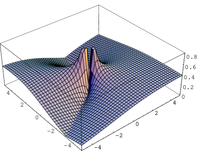
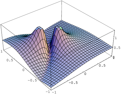
Figure 2: Left panel: The function $A$ defined in Eq. (29) that quantifies the deviation of the approximate $|\beta_{k}|$ with respect to its exact form. $A$ is depicted as a function of $(R,\theta)$ that parameterize the initial conditions ($C_{1},C_{2}$) of the exact solution. Right panel: zoom around the origin in order to unveil the two peaks structure.

We see that the error for large values of $\rho$ is less than $\sim 40\,$% and is constant, i.e. the offset between the two Bogoliubov coefficients does not depend on $\rho$ and $\Phi$ in a first approximation. For $\rho\sim 0$, the error increases to 1; this artefact comes from the fact that the minima where the two Bogoliubov coefficients vanish are slightly offset one from the other. If one coefficient vanishes while the other remains finite and non-zero, then the value of $A$ is pushed toward one, $A\rightarrow 1$. This error however is of no consequence for what follows. Indeed we will not be interested in the location of the minimum but in the behavior of $\beta_{k}$ around the minimum and far from the minimum. As is obvious from Fig. 2, these behaviors match closely in both cases and our approximation will be sufficient for our purposes. We have checked that the function $A$ remains the same for other values of $k_{{\rm c}}/H$ which allow numerical calculations, i.e. $k_{{\rm c}}/H\in[10,10^{3}]$.

The situation is in fact very similar to the standard calculation of the power spectrum in an inflationary theory: in principle, one cannot match two different branches at a point where the approximation breaks down (for standard inflation this occurs at first horizon crossing). However, since the approximation is only violated in a small region one expects the corresponding result to be correct at leading order. This is indeed the case for inflation for which the amplitude of the spectrum is predicted up to a factor of order unity and the spectral slope is unchanged by the matching. Here we also find that $|\beta_{k}^{\rm(approx)}|={\cal O}(1)|\beta_{k}^{\rm(exact)}|$.

III.1.3 Fine-tuning of the initial conditions

Since we have demonstrated that the approximation to $|\beta_{k}|$ is quite reasonable, we now study the behavior of Eq. (18) for more realistic values of the ratio $k_{{\rm c}}/H$. The Bogoliubov coefficient possesses an absolute minimum with $\beta_{k}=0$ located at

$$\rho_{\rm min}^{4}=\frac{\pi^{2}J^{2}}{JN-K^{2}}\,,\quad\cos\Phi_{\rm min}=\frac{K}{\sqrt{JN}}\,,$$ (30)

using the notations defined previously. One should not be surprised to find a minimum with $\beta_{k}=0$ since one can express the matching of the two branches of the solution and their first derivatives at $\eta_{\rm m}$ as two equations relating the coefficients $A_{1}(k)$ and $A_{2}(k)$ as a function of $\alpha_{k}$ and $\beta_{k}$ and find a solution with $\beta_{k}=0$. The Wronskian normalization condition is always satisfied by both branches of the solution. This solution with initial conditions ($\rho_{\rm min}$, $\Phi_{\rm min}$) corresponds to a choice of initial data such that at late times, when modes have exited from the tail, their quantum state is that of an adiabatic vacuum. Note therefore that there is no naturalness in choosing these initial conditions since the adiabatic vacuum is only a late time consequence of such initial data. Furthermore one can show that for generic initial data, the state of the quantum field at late times is not an adiabatic vacuum, hence quanta have been produced.

Indeed the behavior of $|\beta_{k}|^{2}$ around this absolute minimum can easily be established. From a Taylor expansion, one obtains

$$|\beta_{k}|^{2}\simeq\frac{N}{\sqrt{2}}(\rho-\rho_{\rm min})^{2}\,,\quad|\beta_{k}|^{2}\simeq\frac{\pi^{4}}{16}J^{2}N^{2}(\Phi-\Phi_{\rm min})^{2}\,.$$ (31)

For a crude order of magnitude estimate, one can develop the Bessel functions to first order in the small argument limit $e^{y_{\rm m}}=2\sqrt{2}k_{{\rm c}}/K_{+}\ll 1$ (more exactly, for de Sitter inflation and $k_{\rm c}=M_{\rm Pl}$, one has $k_{\rm c}/K_{+}\simeq 0.06$). This leads to $J\simeq 1/16+{\cal O}(k_{{\rm c}}^{2}/K_{+}^{2})$ and $N\simeq\ln^{2}(\sqrt{2}k_{\rm c}/K_{+})/(4\pi^{2})(K_{+}^{2}/k_{{\rm c}}^{2})+{\cal O}(k_{{\rm c}}^{0}/K_{+}^{0})$. Thus in order to avoid a back-reaction problem, the initial conditions $\rho$ and $\Phi$ must not differ too much from $\rho_{\rm min}$ and $\Phi_{\rm min}$ which lead to $\beta_{k}=0$ (hence a zero amount of energy density created). More precisely, the energy density produced is of the order of the background energy density, i.e. ${\rm d}\Omega_{\omega}/{\rm d}\ln(k_{\rm phys})=1$, when $\rho$ or $\Phi$ respectively depart from the minimum by amounts $\delta\rho$ or $\delta\Phi$ given by:

$$\delta\rho\simeq{\cal O}\biggl{[}\frac{H}{M_{\rm Pl}}\ln^{-1}\biggl{(}\frac{M_{\rm Pl}}{H}\biggl{)}\biggr{]}\,,\quad\delta\Phi\simeq{\cal O}\biggl{[}\frac{H}{M_{\rm Pl}}\ln^{-2}\biggl{(}\frac{M_{\rm Pl}}{H}\biggl{)}\biggr{]}\,.$$ (32)

Here we assumed $k_{\rm c}=M_{\rm Pl}$. Hence the corresponding fine-tuning of the initial conditions is of order $H/M_{\rm Pl}$ (if one assumes a uniform measure in $\rho$ and $\Phi$ in parameter space).

One should note that the above constraint is valid for a given co-moving wave-number $k$ and has been calculated at a time when $k/a=k_{\rm c}$. Since the fractional density parameter of quanta extracted out of the vacuum ${\rm d}\Omega_{\omega}/{\rm d}\ln(k_{\rm phys})$ must be smaller at all times during inflation, i.e. for a range of co-moving wave-numbers $k$ since $k$ and $\eta$ can be related by the above constraint $k/a=k_{\rm c}$, the above constraint on $\rho_{\rm min}$ and $\Phi_{\rm min}$ rather applies to a continuum of values of co-moving wave-numbers. In other words one does not have to fine-tune two parameters characterizing the initial data but a whole continuum of parameters, i.e. the functions $\rho_{\rm min}(k)$ and $\Phi_{\rm min}(k)$ themselves. The dependence in $k$ of these functions is hidden in the argument of the Bessel and Neumann functions ${\rm e}^{y_{\rm m}}$, since $y_{\rm m}$ depends on $k$.

III.2 Non conformal coupling: $\xi\not=1/6$

One can also perform a similar calculation of the Bogoliubov coefficient when the coupling is no longer conformal $\xi\neq 1/6$. In this case the calculation can be performed analytically for all background scale factors. For the sake of simplicity we choose minimal coupling $\xi=0$ but this can be trivially expanded to various choices of the coupling to gravity, and does not modify the conclusions we derive below.

If $\xi=0$, the evolution of the modes is dominated by $a^{\prime\prime}/a$ in the tail, i.e. when $\omega_{\rm phys}\ll H$ ($k_{\rm phys}\gg k_{\rm c}$), and the solution can be written as:

$$\mu_{k}(\eta)\,=\,\frac{1}{\sqrt{2k}}\left[C_{+}(k)\frac{a(\eta)}{a_{\rm i}}-C_{-}(k)\frac{a_{\rm i}}{\eta_{\rm i}}a(\eta)\int_{\eta_{\rm i}}^{\eta}\frac{{\rm d}\tau}{a^{2}(\tau)}\right],$$ (33)

where $C_{+}(k)$ and $C_{-}(k)$ are two dimensionless $k-$dependent constants, and $\eta_{\rm i}$ is some initial conformal time. One can check that this solution and the power-laws given in Eq. (4) are the same. Here one cannot choose the time of matching $\eta_{\rm m}$ to the WKB solution, since the matching has to be done when $\Omega_{k}=0$, i.e. when $\omega_{k}^{2}=a^{\prime\prime}/a$ or $k_{\rm phys}=K_{+}$. In the region $\omega_{\rm phys}\gg H$, i.e. for $\eta\gg\eta_{\rm m}$, the WKB approximation is valid as we have seen before, and the matching to the WKB form is justified at $\eta=\eta_{\rm m}(k)$. For a given wave-number $k$, we are free to set $\eta_{\rm i}=\eta_{\rm m}$, since this amounts to a redefinition of the constants $C_{+}(k)$ and $C_{-}(k)$ by a function of $k$. The matching at $\eta_{\rm m}$ then gives:

$$\alpha_{k}\,=\,\frac{i}{\sqrt{4k\omega_{k}}}\left[C_{+}\biggl{(}\gamma_{k}^{*}+\frac{a^{\prime}}{a}\biggr{)}-\frac{C_{-}}{\eta_{\rm m}}\right],\quad\quad\beta_{k}\,=\,\frac{-i}{\sqrt{4k\omega_{k}}}\left[C_{+}\biggl{(}\gamma_{k}+\frac{a^{\prime}}{a}\biggr{)}-\frac{C_{-}}{\eta_{\rm m}}\right]\,,$$ (34)

with the function $\gamma_{k}\equiv(\omega^{\prime}/2\omega)+i\omega$ as above [see Eq. (16)] and where all quantities in the above two equations are understood to be taken at $\eta=\eta_{\rm m}(k)$. In particular, at time $\eta_{\rm m}$, $\omega_{k}^{2}=a^{\prime\prime}/a=(1+\beta)a_{\rm m}^{2}H_{\rm m}^{2}/\beta$. Since $k_{\rm phys}\gg k_{\rm c}$ at $\eta_{\rm m}$ one can use the limiting form of $\omega_{\rm phys}$ given in Eq. (9), hence:

$$\gamma_{k}+\frac{a^{\prime}}{a}\simeq a_{\rm m}H_{\rm m}\left(\frac{K_{+}}{4k_{\rm c}}+1+i\sqrt{\frac{1+\beta}{\beta}}\right).$$ (35)

The constants $C_{+}(k)$ and $C_{-}(k)$ are related to one another by the normalization of the mode functions: $\mu_{k}\mu_{k}^{*\prime}-\mu_{k}^{\prime}\mu_{k}^{*}=i$, which gives:

$$C_{+}(k)\,=\,-\beta\frac{K_{+}}{H_{\rm m}r\sin\Phi},$$ (36)

and as before we keep $r\equiv|C_{-}(k)|$ and $\Phi={\rm arg}[C_{-}(k)]$ as the two independent parameters characterizing the choice of initial data. One finally derives the squared modulus of the Bogoliubov coefficient $\beta_{k}$ as:

$$|\beta_{k}|^{2}\,=\,\frac{1}{r^{2}\sin^{2}\Phi}\frac{\beta^{2}}{4}\sqrt{\frac{\beta}{\beta+1}}\frac{K_{+}}{H_{\rm m}}\left[\left(1+\frac{K_{+}}{4k_{\rm c}}\right)^{2}+\frac{1+\beta}{\beta}\right]+\frac{r^{2}}{4\beta^{2}}\sqrt{\frac{\beta}{1+\beta}}\frac{H_{\rm m}}{K_{+}}-\frac{1}{2}\sqrt{\frac{\beta}{1+\beta}}\left(1+\frac{K_{+}}{4k_{\rm c}}\right){\rm cot}\Phi-\frac{1}{2}.$$ (37)

Since $K_{+}/H_{\rm m}$ is a large number, in the following we use the rescaled variable $\rho\equiv r\sqrt{H/K_{+}}$ instead of $r$. Equation (37) above is particularly attractive because it has exactly the same functional shape as Eq. (18). It allows us to understand analytically the behavior of the amount of energy density produced in modes with $k_{\rm phys}\sim k_{\rm c}$ as a function of the initial data. The occupation number $|\beta_{k}|^{2}$ has an absolute minimum located at:

$$\rho_{\rm min}=|\beta|\biggl{(}\frac{\beta}{1+\beta}\biggr{)}^{1/4}\sqrt{\biggl{(}1+\frac{K_{+}}{4k_{\rm c}}\biggr{)}^{2}+\frac{1+\beta}{\beta}}\,,\quad\cos\Phi_{\rm min}\,=\,\frac{1+K_{+}/(4k_{\rm c})}{\sqrt{\left[1+K_{+}/(4k_{\rm c})\right]^{2}+(1+\beta)/\beta}}.$$ (38)

As before the occupation number vanishes exactly at this minimum, but the back-reaction problem cannot be avoided for generic initial conditions. In the present case it is not possible to make a sensible contour plot of ${\rm d}\Omega_{\omega}/{\rm d}\ln(k_{\rm phys})$ since this function changes by many orders of magnitude over very small intervals of $\rho,\Phi$. Therefore, we take a conservative approach in which we calculate $|\beta_{k}(\rho)|^{2}$ as a function of $\rho$ for the values of $\Phi$ that minimize this quantity at each $\rho$. We also evaluate $|\beta_{k}(\Phi)|^{2}$ as a function of $\Phi$ for the values of $\rho$ that minimize this quantity at each $\Phi$. In other words, we solve $\partial_{\Phi}|\beta_{k}|^{2}=0$ for $\Phi$ as a function of $\rho$ and $\partial_{\rho}|\beta_{k}|^{2}=0$ for $\rho$ as a function of $\Phi$:

$$\Phi_{\rm min}(\rho)=\tan^{-1}\biggl{\{}\frac{\beta^{2}}{\rho^{2}}\frac{[1+K_{+}/(4k_{\rm c})]^{2}+(1+\beta)/\beta}{1+K_{+}/(4k_{\rm c})}\biggr{\}}\,,\quad\rho_{\rm min}^{4}(\Phi)\,=\,\frac{\beta^{4}}{\sin^{2}\Phi}\left[\left(1+\frac{K_{+}}{4k_{\rm c}}\right)^{2}+\frac{1+\beta}{\beta}\right],$$ (39)

Figure 3: Left panel: the solid line represents $\log_{10}\left(|\beta_{k}|^{2}/|\beta_{k}^{\rm max}|^{2}\right)\equiv\log_{10}\left[{\rm d}\Omega_{\omega}/{\rm d}\ln(k_{\rm phys})\right]$ plotted as a function of the rescaled variable $\rho$ characterizing the initial data. This plot corresponds to an inflationary era with a de Sitter metric, and Hubble parameter $\sim 10^{-6}M_{{\rm Pl}}$. The other parameter of initial data is $\Phi=\Phi_{\rm min}$. Allowed regions correspond to $\log_{10}\left(|\beta_{k}|^{2}/|\beta_{k}^{\rm max}|^{2}\right)<0$, and are peaked around a particular value of $\rho$. The minimum is in fact $|\beta_{k}|^{2}=0$, corresponding to $\log_{10}\left(|\beta_{k}|^{2}/|\beta_{k}^{\rm max}|^{2}\right)=-\infty$, but cannot be seen in the figure due to insufficient resolution. The dotted line provides a continuation of the numerical result to the analytical value at that point. In most of parameter space, the energy density is too large by $\sim$10 orders of magnitude. Right panel: Same as left panel for $H_{0}\sim 10^{-61}M_{{\rm Pl}}$ in a matter dominated era. In nearly all of parameter space the energy density is too large by $\sim 122$ orders of magnitude .

Figure 4: Left panel: $\log_{10}\left(|\beta_{k}|^{2}/|\beta_{k}^{\rm max}|^{2}\right)\equiv\left[{\rm d}\Omega_{\omega}/{\rm d}\ln(k_{\rm phys})\right]$ plotted as a function of the phase characterizing the initial data. This plot corresponds to an inflationary era with a de Sitter metric, and Hubble parameter $\sim 10^{-6}M_{{\rm Pl}}$. As indicated in the text, the other parameter of initial data (a modulus) has been eliminated for the phase $\Phi$ by minimizing $|\beta_{k}|^{2}$. Allowed regions correspond to $\log_{10}\left(|\beta_{k}|^{2}/|\beta_{k}^{\rm max}|^{2}\right)<0$, and are seen to be peaked around a particular value of $\Phi$. The plot is symmetric in the interchange $\Phi\leftrightarrow\Phi+\pi$. Note that the ordinate scale is in $\log_{10}$: in most of parameter space, the energy density is too large by $\sim$10 orders of magnitude. Right panel: Same as left panel for $H_{0}\sim 10^{-61}M_{{\rm Pl}}$ in a matter dominated era. In nearly all of parameter space the energy density is too large by $\sim 122$ orders of magnitude, i.e. ${\rm d}\Omega_{\omega}/{\rm d}\ln(k_{\rm phys})\sim M_{{\rm Pl}}^{4}$.

and plot ${\rm d}\Omega_{\omega}/{\rm d}\ln(k_{\rm phys})$ for $|\beta_{k}[\rho,\Phi_{\rm min}(\rho)]|^{2}$ in Figs. 3 and $|\beta_{k}[\rho_{\rm min}(\Phi),\Phi]|^{2}$ in Figs. 4 (for respectively de Sitter inflation and today). One clearly sees from these figures that ${\rm d}\Omega_{\omega}/{\rm d}\ln(k_{\rm phys})\sim M_{{\rm Pl}}^{2}/H^{2}$ for most values of $\Phi$, which corresponds to our previous expectations, i.e. the amount of energy density created in quanta with $k_{\rm phys}\sim k_{\rm c}\sim M_{{\rm Pl}}$ is of order $M_{{\rm Pl}}^{4}$. The behavior of $|\beta_{k}|^{2}$ around the local minimum can be studied in the same way as before and one obtains:

$$|\beta_{k}|^{2}(\rho) \simeq \frac{1}{\beta^{2}}\biggl{(}\frac{\beta}{1+\beta}\biggr{)}^{1/2}(\rho-\rho_{\rm min})^{2}\,,\quad\quad(\rho\sim\rho_{\rm min})\,,$$ (40)

$$|\beta_{k}|^{2}(\Phi) \simeq \frac{1}{4}\biggl{(}\frac{\beta}{1+\beta}\biggr{)}^{2}\left[\left(1+\frac{K_{+}}{4k_{\rm c}}\right)^{2}+\frac{1+\beta}{\beta}\right]^{2}\left(\Phi-\Phi_{\rm min}\right)^{2}\,,\quad\quad(\Phi\sim\Phi_{\rm min}).$$ (41)

If we write the value $|\beta_{k}|^{2}_{\rm max}$ such that ${\rm d}\Omega_{\omega}/{\rm d}\ln(k_{\rm phys})=1$ (i.e. similar amount of energy created in quanta with $k_{\rm phys}\sim k_{\rm c}$ than in the background), then this value is reached if $\rho$ and $\Phi$ departs from $\rho_{\rm min}$ and $\Phi_{\rm min}$ by an amount $\delta\rho$, $\delta\Phi$, with:

$$\delta\rho\sim{\cal O}\left(\frac{H}{M_{{\rm Pl}}}\right)\,,\quad\delta\Phi\sim{\cal O}\left[\frac{H}{M_{{\rm Pl}}}\ln^{-2}\left(\frac{M_{{\rm Pl}}}{H}\right)\right].$$ (42)

In other words, the fine-tuning necessary to avoid back-reaction is of order $\sim\delta\Phi\sim\delta\rho\sim H/M_{{\rm Pl}}$ (neglecting the ln term). During inflation $H/M_{{\rm Pl}}\sim 10^{-6}$, and today $H/M_{{\rm Pl}}\sim 10^{-61}$. Although the fine-tuning can be considered as not too severe during inflation, we see that, during the matter epoch, it is as severe as the usual fine-tuning of the cosmological constant problem. Therefore, the scenario of Refs. MBK01 ; BFM02 ; BM02 does not improve the situation.

At this point, it should be emphasized that the above problem is a generic feature of the dispersion relation used in Refs. MBK01 ; BFM02 ; BM02 . In order for the trans-Planckian effects to modify the power spectrum of the fluctuations, the physical modes of interest must spend some time in a region where the WKB approximation is violated. As already mentioned, this implies production of particles and the energy density associated to these particles must not exceed the background energy density. This implies some constraints on the occupation number $|\beta_{k}|^{2}$. It has been shown in Ref. S01 that these constraints are quite stringent if the production is taking place today. Usually, these tight constraints can be avoided by requiring that the violation only occurs during inflation where the problem is less severe. This can be achieved if the dispersion relation is such that $\omega_{\rm phys}\gg H$ for all trans-Planckian wave-numbers, with $H$ the Hubble constant some unspecified time after inflation. Such an example is provided in Fig. 2 of Ref. LMMU01 . Then as was argued in the discussion following Eq. (9) the WKB approximation should be valid at all times after inflation and adiabaticity restored. Here however, since $\omega_{\rm phys}\rightarrow 0$ as $k_{\rm phys}\rightarrow+\infty$, there is at all times a region where the WKB is violated. Therefore the class of dispersion relations used in Refs. MBK01 ; BFM02 ; BM02 suffer in a generic way from the problem discussed in Ref. S01 .

Furthermore, we also note as previously that the above calculation of the fine-tuning holds for a given co-moving wave-number $k$. Similar constraints apply for other wave-numbers but the values of $\Phi_{\rm min}$ and $\rho_{\rm min}$ are shifted from the above [notably because of the choice $\eta_{\rm i}=\eta_{\rm m}(k)$]. Therefore one must not only pick one right value of $\Phi$ to one part in $\sim M_{{\rm Pl}}/H$, but a whole continuum of values of $\Phi(k)$ such that back-reaction is avoided for all of these values.

IV Equation of state

Up to now we have argued that: (i) in the scenario proposed in Refs. MBK01 ; BFM02 ; BM02 there is no preferred initial vacuum state, hence all conclusions drawn depend on the ad-hoc choice of initial data; (ii) for arbitrary values of the two parameters characterizing this choice of initial data one finds that energy in excess of the background energy density is produced due to the non adiabatic evolution of modes in the tail.

In a separate publication, we have constructed an effective energy-momentum tensor for scalar field theories with non-linear dispersion relations, and we have shown that dispersion relations of the form of that proposed in Refs. MBK01 ; BFM02 ; BM02 generically led to the wrong equation of state. This finding has been challenged by Bastero-Gil and Mersini recently, who argue that the energy-momentum tensor we have constructed is ill-defined as it (supposedly) is not divergenceless.

Explicitly, in Ref. LMMU01 , the vev for the energy density and pressure are given by

$$\langle\rho\rangle = \frac{1}{4\pi^{2}a^{4}}\int{\rm d}kk^{2}\left[a^{2}\left|\left(\frac{\mu_{k}}{a}\right)^{\prime}\right|^{2}+\omega^{2}(k)\left|\mu_{k}\right|^{2}\right],$$ (43)

$$\langle p\rangle = \frac{1}{4\pi^{2}a^{4}}\int{\rm d}kk^{2}\left[a^{2}\left|\left(\frac{\mu_{k}}{a}\right)^{\prime}\right|^{2}+\left(\frac{2}{3}k^{2}\frac{{\rm d}\omega^{2}}{{\rm d}k^{2}}-\omega^{2}\right)\left|\mu_{k}\right|^{2}\right],$$ (44)

and the integrals extend from $0$ to $+\infty$. Reference BM02 claims that $\langle\rho\rangle^{\prime}+3{\cal H}\langle\rho+p\rangle\neq 0$, with ${\cal H}\equiv a^{\prime}/a$. However, noting that the co-moving frequency $\omega(k)=a\omega_{\rm phys}(k_{\rm phys})$, a straightforward calculation gives:

$$\langle\rho\rangle^{\prime} = \frac{1}{4\pi^{2}a^{4}}\int{\rm d}kk^{2}\biggl{\{}\left[\mu_{k}^{\prime\prime}-{\cal H}\mu_{k}^{\prime}+\left({\cal H}^{2}-{a^{\prime\prime}\over a}\right)\mu_{k}\right]\left(\mu_{k}^{*\prime}-{\cal H}\mu_{k}^{*}\right)+\left(\mu_{k}^{\prime}-{\cal H}\mu_{k}\right)\left[\mu_{k}^{*\prime\prime}-{\cal H}\mu_{k}^{*\prime}+\left({\cal H}^{2}-{a^{\prime\prime}\over a}\right)\mu_{k}^{*}\right]$$ (45)

$$-4{\cal H}\left|\mu_{k}^{\prime}-{\cal H}\mu_{k}\right|^{2}+\omega^{2}(k)\left(\mu_{k}^{\prime}\mu_{k}^{*}+\mu_{k}\mu_{k}^{*\prime}\right)-2{\cal H}k^{2}{{\rm d}\omega^{2}\over{\rm d}k^{2}}|\mu_{k}|^{2}-2{\cal H}\omega^{2}(k)|\mu_{k}|^{2}\biggr{\}}$$

$$= \frac{1}{4\pi^{2}a^{4}}\int{\rm d}kk^{2}\biggl{\{}\left(\mu_{k}^{\prime\prime}-{a^{\prime\prime}\over a}\mu_{k}\right)\left(\mu_{k}^{*\prime}-{\cal H}\mu_{k}^{*}\right)+\left(\mu_{k}^{\prime}-{\cal H}\mu_{k}\right)\left(\mu_{k}^{*\prime\prime}-{a^{\prime\prime}\over a}\mu_{k}^{*}\right)-6{\cal H}\left|\mu_{k}^{\prime}-{\cal H}\mu_{k}\right|^{2}$$

$$+\omega^{2}(k)\left[\mu_{k}\left(\mu_{k}^{*\prime}-{\cal H}\mu_{k}^{*}\right)+\mu_{k}^{*}\left(\mu_{k}^{\prime}-{\cal H}\mu_{k}\right)\right]-2{\cal H}k^{2}{{\rm d}\omega^{2}\over{\rm d}k^{2}}|\mu_{k}|^{2}\biggr{\}}$$

$$= \frac{1}{4\pi^{2}a^{4}}\int{\rm d}kk^{2}\biggl{(}-6{\cal H}\left|\mu_{k}^{\prime}-{\cal H}\mu_{k}\right|^{2}-2{\cal H}k^{2}{{\rm d}\omega^{2}\over{\rm d}k^{2}}|\mu_{k}|^{2}\biggr{)},$$

where the field equation $\mu_{k}^{\prime\prime}-(a^{\prime\prime}/a)\mu_{k}=-\omega^{2}(k)\mu_{k}$ has been used in the last step. Since

$$3{\cal H}\langle\rho+p\rangle\,=\,\frac{1}{4\pi^{2}a^{4}}\int{\rm d}kk^{2}\left(6{\cal H}\left|\mu_{k}^{\prime}-{\cal H}\mu_{k}\right|^{2}+2{\cal H}k^{2}{{\rm d}\omega^{2}\over{\rm d}k^{2}}|\mu_{k}|^{2}\right)\,,$$ (46)

the energy conservation condition $\langle\rho\rangle^{\prime}+3{\cal H}\langle\rho+p\rangle=0$ is trivially satisfied.

We take advantage of this Section to point out that the energy-momentum tensor we have constructed in a previous publication LMMU01 is well behaved and the construction is entirely consistent. In effect we constructed a generally covariant Lagrangian for a scalar field with a non-linear dispersion relation. The breaking of the Lorentz invariance is explicited by introducing a dynamical four-vector $u^{\mu}$ in the Lagrangian whose role is to define the preferred rest frame while preserving general covariance at the same time, following previous work by Jacobson and Mattingly JM01 (see also references therein). The energy-momentum tensor derived by varying the action with respect to the metric is the sum of the energy-momentum tensor of the scalar field and that of $u^{\mu}$. We have restricted ourselves to FLRW space-times by choosing $u^{\mu}=(-1,0,0,0)$. This approach is consistent as $u^{\mu}$ satisfies its field equation [see Eq. (15) in Ref. LMMU01 ], and the scalar field also satisfies its field equation. In FRLW space-time, the energy-momentum tensor of the four-vector (i.e. the part which depends only on $u^{\mu}$) vanishes since $u^{\mu}$ is constant LMMU01 , hence the remainder is the scalar field energy-momentum tensor, which is conserved as shown above. We consider this scalar field as a test field, which we quantize on the curved background. The dynamics of the background can be specified by adding matter fields to the action without modifying our approach. Indeed the matter field energy-momentum tensor will be separately conserved. Therefore our earlier criticisms on the equation of state of the trans-Planckian modes apply.

We also note that a recent paper by Frampton F02 argues that by adding higher order terms of the form $u^{\mu}{\cal D}^{2n}u_{\mu}$ in the effective Lagrangian, one can obtain a correct equation of state, i.e. similar to that of vacuum. Here ${\cal D}^{2}$ denotes a three-dimensional Laplacian expressed in a generally covariant way on space-like hyper-surfaces (see Refs. JM01 ; LMMU01 for explicit definitions). The choice $u^{\mu}=(-1,0,0,0)$ then reduces this term to the usual three-dimensional Laplacian on constant time hyper-surfaces for FLRW space-times. However, as should be obvious, the only terms that can enter the energy-momentum tensor via this new term always contain derivatives of the form ${\cal D}^{2n}u^{\mu}$ when $n\geq 2$. Those terms vanish when one picks $u^{\mu}$ to be constant as above. For $n=1$, i.e. the lowest order term of the expansion, one can check that the variation of ${\cal D}^{2}u^{\mu}$ with respect to the metric or its first derivative always induces a term proportional to a derivative of $u^{\mu}$ that is either spatial or temporal. This calculation can be found in Eqs. (B3) and (B4) of Ref. LMMU01 (the substitution $\phi\rightarrow u^{\mu}$ in this calculation can be made without changing the result since the equation is written in a generally covariant way). Therefore we conclude that the addition of terms proposed by Frampton cannot lead to any difference with respect to the energy-momentum tensor we proposed earlier. Hence such terms cannot account straightforwardly for a vacuum-like equation of state in this scenario.

The difference with the conclusion of Ref. F02 probably lies in the choice of normalization of $u^{\mu}$: Ref. F02 claims that, in a cosmological context, $u^{\mu}u_{\mu}-a^{-2}=0$ ($a$ is the scale factor). However, $u^{\mu}u_{\mu}$ is a scalar, while $a^{-2}$ is the component of a rank two tensor so that this choice of normalization is manifestly not covariant. Of course, it can be made covariant at the expense of the introduction of a second vector field but this does not seem to be the case in Ref. F02 . This implies that the Lagrangian proposed by Frampton is generally not covariant. Of course the correct normalization for $u^{\mu}$ in a cosmological context is always $u^{\mu}u_{\mu}-1=0$ (up to the sign convention), and $u^{\mu}$ can be written as $(-1/a,0,0,0)$ if the FRLW metric is written in terms of conformal time, or $(-1,0,0,0)$ if the metric is written in terms of cosmic time.

To finish, let us also note that it is claimed in Ref. MBK01 that “the tail modes are still frozen at present… Thus the energy of the tail is a contribution to the dark energy of the Universe: up to the present it has the equation of state of a cosmological constant term”. Here, that the tail modes are frozen means $(\mu_{k}/a)^{\prime}\sim 0$, the solution to the field equation when the term $a^{\prime\prime}/a$ dominates (for $\xi=0$). But there is no logical relationship between these modes being frozen and the equation of state being that of a cosmological constant. As a matter of fact the equation of state of the modes of wavelengths larger than the horizon size for a scalar field with a linear dispersion relation takes the form $p=-\rho/3$. The derivation of the equation of state requires to define correctly a stress-energy tensor when such non-linear dispersion relations are taken into account (and thus when Lorentz invariance is broken) as we did in Ref. LMMU01 . Note also that there is a contradiction between the above claim of Ref. MBK01 and the whole content of the recent paper by Bastero-Gil and Mersini BM02 which calculates the equation of state of the trans-Planckian modes and finds that it is not the equation of state of the vacuum but that it approaches it only at late times.

V Conclusions

In this article, we have examined in detail the scenario proposed in Refs. MBK01 ; BFM02 ; BM02 which attributes the dark energy to the properties of a scalar field with a dispersion relation that decreases exponentially with trans-Planckian wave-number $k_{\rm phys}\gtrsim k_{\rm c}\sim M_{\rm Pl}$. We have demonstrated that this mechanism does not work, mainly for two reasons. (i) The mode function of the scalar field does not behave as a plane wave as $\eta\rightarrow-\infty$ in the so-called “tail” (i.e., the part of the non-linear dispersion relation where $\omega_{\rm phys}\ll H$ and $k_{\rm phys}\gg M_{{\rm Pl}}$). This implies that there is no definite prescription for constructing a well-defined initial vacuum state, hence that the choice of initial data is entirely arbitrary. This situation is similar to the problem of setting initial data for cosmological perturbations in the absence of an accelerated expansion era (but with linear dispersion relations), in which case the data would have to be specified on super-horizon scales where the mode function does not oscillate and is frozen by the expansion. In the scenario of Refs. MBK01 ; BFM02 ; BM02 the WKB approximation is not valid at all times for modes in the tail. This explains that the notion of adiabatic vacuum cannot be used to set up initial data and the initial state proposed in Ref. MBK01 is thus ad-hoc. It also brings us to the second objection against this scenario: (ii) since all modes originate in the tail of the dispersion relation, the breakdown of the WKB approximation for a given physical wave-number at early times implies the continuous production of a substantial number of quanta with physical wave-numbers $\gtrsim k_{\rm c}$. The breakdown of the WKB approximation can indeed be seen as the signal of a strongly non-adiabatic evolution which is generically associated with particle production in expanding space-times. We have calculated the amount of energy density produced in modes of physical wave-number $k_{\rm c}$ as a function of the two parameters that characterize the (arbitrary) choice of initial data. We have shown that this energy density is generically of order $M_{{\rm Pl}}^{4}$. The production of energy density in quanta with wave-numbers $\sim M_{{\rm Pl}}$ in excess of the background energy density $\sim H^{2}M_{{\rm Pl}}^{2}$ implies the breakdown of the perturbative semi-classical framework used for the calculation, and renders all claims irrelevant. There is a small region of parameter space in which this energy density can be tuned down to zero, but the fine-tuning in the choice of initial data is of order $H/M_{{\rm Pl}}$. Such a fine-tuning at the time of inflation is of order $\sim 10^{-6}$ and is probably acceptable, but today, it is of the same order as the celebrated fine-tuning of the cosmological constant problem.

References

- (1) L. Mersini, M. Bastero-Gil, and P. Kanti, Phys. Rev. D 64, 043508 (2001).
- (2) M. Bastero-Gil, P. Frampton and L. Mersini, Phys. Rev. D 65, 106002 (2002).
- (3) M. Bastero-Gil and L. Mersini, arXiv:hep-ph/0205271.
- (4) W. Unruh, Phys. Rev. D 51, 2827 (1995); S. Corley and T. Jacobson, Phys. Rev. D 54, 1568 (1996).
- (5) J. Martin and R. H. Brandenberger, Phys. Rev. D 63, 123501 (2001); R. H. Brandenberger and J. Martin, Mod. Phys. Lett. A 16, 999 (2001); J. C. Niemeyer, Phys. Rev. D 63, 123502 (2001).
- (6) M. Lemoine, M. Lubo, J. Martin, and J.-P. Uzan, Phys. Rev. D 65, 023510 (2001).
- (7) N. D. Birrell and P. C. W. Davies, “Quantum fields in curved space”, Cambridge University Press (1982).
- (8) A. A. Starobinsky, Pisma Zh. Eksp. Teor. Fiz. 73, 415 (2001).
- (9) M. Abramowitz and A. I. Stegun, “Handbook of mathematical functions”, Dover, New-York (1965).
- (10) P. Frampton, arXiv:astro-ph/0209037.
- (11) J. Martin and D. J. Schwarz, arXiv:astro-ph/0210090.
- (12) http://functions.wolfram.com
- (13) T. Jacobson and D. Mattingly, arXiv:gr-qc/0007031; T. Jacobson and D. Mattingly, Phys. Rev. D 63, 041502(R) (2001).