Dynamical vacuum selection in field theories with flat directions in their potential

Abstract

In this paper we show that in field theories with topologically stable kinks and flat directions in their potential, a so-called dynamical vacuum selection (DVS) takes place in the non-trivial, soliton sector of the theory. We explore this DVS mechanism using a specific model. For this model we show that there is only a static kink solution when very specific boundary conditions are met, very similar to the case of vortices in two dimensions. In the case of other boundary conditions a scalar cloud is expelled to infinity, leaving a static kink behind. Other circumstances under which DVS may or may not take place are discussed as well.

1 Introduction

In this paper we examine topological defects in theories with flat directions in their potential. Flat directions in the scalar potential are quite natural in the context of supersymmetric models. As was noticed in [1], in spite of the fact that a model does allow topologically stable vortices, not all admissible boundary conditions in a given model with flat directions, are compatible with the existence of a static vortex solution. In [2] such vortices in theories with flat directions were studied, and it was shown that in the presence of a topologically stable vortex, a specific vacuum is dynamically selected. In this paper we focus on the one dimensional case and show that also for theories in one dimension with flat directions not all boundary conditions allow the existence of a static kink. We will show that a specific vacuum is dynamically selected in the presence of such a kink or domain wall. Although we will use a specific model, it will become clear that dynamical vacuum selection (DVS) is a general feature for theories with flat directions in one dimension.
To be a bit more specific we will discuss a class of models which have two copies of a scalar Higgs field and a potential of the following form,

$$V(\phi_{1},\phi_{2})=\frac{\lambda}{4}(\phi_{1}^{2}-\phi_{2}^{2}-f^{2})^{2}\quad,$$ (1)

in analogy with the model studied in [2].

In section 2 we focus on the one dimensional model, in section 3 we comment on the two dimensional model which was discussed in [2], and in section 4, we show with the help of a Bogomolny [3] type argument that there is no DVS in the three dimensional case, as was already anticipated in [2]. We end the paper with some conclusions and a brief discussion.

2 Dynamical vacuum selection (DVS) in 1 dimension

In this section we investigate DVS in a specific one dimensional model. First we introduce the model, subsequently we prove that there is only a static kink solution for a very specific non trivial boundary condition out of a continuum of allowed boundary conditions. Finally we investigate the kink dynamics if this specific boundary condition is not met and we find that indeed the DVS mechanism becomes operative.

2.1 The model

We consider a model with two real scalar fields and a potential which allows for the formation of topologically stable kinks and which furthermore features a flat direction.
The model is given by:

$$\mathcal{L}=\int dx\{\frac{1}{2}(\partial_{\mu}\phi_{1})^{2}+\frac{1}{2}(\partial_{\mu}\phi_{2})^{2}-\frac{\lambda}{4}(\phi_{1}^{2}-\phi_{2}^{2}-f^{2})^{2}\}\quad,$$ (2)

with $\phi_{1}$ and $\phi_{2}$ two real scalar fields.

It is quite clear that this model contains topologically stable kinks, which have to satisfy the spatial boundary conditions $\phi_{1}(\pm\infty)=\sqrt{f^{2}+\phi_{2}(\pm\infty)^{2}}$ and $\phi_{1}(\mp\infty)=-\sqrt{f^{2}+\phi_{2}(\mp\infty)^{2}}$. Note that the boundary values of $\phi_{2}$ do not influence the topological charge of the kink. Thus there is a two parameter class of topologically stable kinks present in this model, labeled by $(\phi_{2}(-\infty);\phi_{2}(+\infty))$. In the next section we investigate the class of static kink solutions in this model when real space is taken infinite, this class as we will show is in fact very small.

2.2 Static kinks

Naively one might expect to be able to find a static kink solution (assuming real space to be infinite) for any set of the boundary values of $\phi_{2}$ in the topologically nontrivial sector. However this turns out not to be true. What we in fact will show is that there is only one very specific set of boundary values of $\phi_{2}$ for which a static kink solution exists.

To obtain a static configuration, one sets the time derivatives equal to zero and extremizes the resulting Hamiltonian. This Hamiltonian of this model can be interpreted as the action of a point particle in a two dimensional potential, and we may analyze the system through this mechanical analogue. More explicitly, after making the following identifications: $x\to t$, $\phi_{1}\to x$ and $\phi_{2}\to y$, we get the following action:

$$S=\int dt\{\frac{1}{2}(\partial_{t}x)^{2}+\frac{1}{2}(\partial_{t}y)^{2}+\frac{\lambda}{4}(x^{2}-y^{2}-f^{2})^{2}\}\quad.$$ (3)

This system corresponds to a point particle moving in the potential $-\frac{\lambda}{4}(x^{2}-y^{2}-f^{2})^{2}$.

The problem of finding a static kink solution is now translated to finding a solution to the equations of motion of the point particle, which moves from one point on one line of maxima of the potential, $x=\pm\sqrt{f^{2}+y^{2}}$, at $t\to-\infty$ to an other point on the other line of maxima, $x=\mp\sqrt{f^{2}+y^{2}}$, at $t\to\infty$ (see figure 1).

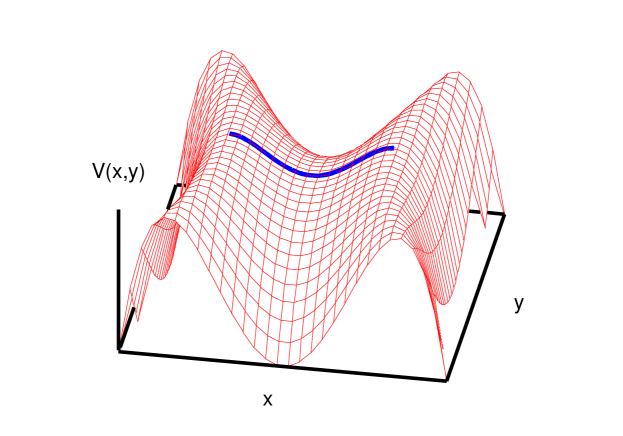
Figure 1: The two dimensional potential for the point particle. The only path satisfying the desired boundary conditions is the path with $y(t)=0$. This path represents the only static kink solution in an infinite space, for which $\phi_{2}(x)=0$.

At $t\to-\infty$ the particle should be at rest in one of the maxima of the potential. At $t\to\infty$ the particle needs to be at rest in one of the other set of maxima of the potential. Obviously there is only one path which satisfies these these boundary conditions and that is the path with $y=0$. Any path starting with $y(t\to-\infty)\neq 0$ in one of the maxima of the potential will never again reach a maximum of the potential. In such a case it is easy to prove that the kinetic energy of the particle associated with component of the motion in the $y$-direction will increase monotonically in time and therefore the particle can never climb out of the potential well again, i.e., will not not able to satisfy the boundary condition at $t\to\infty$. Translating this back to the kink solutions, this means that one can only have a static kink solution if the boundary conditions of $\phi_{2}$ are $\phi_{2}(\pm\infty)=0$ and moreover for the static solution we get $\phi_{2}(x)=0$. Thus the only static kink solution for this model in an infinite space is equal to the usual kink solution.

A crucial step in deriving this result was the infinite size of real space. If space is finite the argument changes dramatically. In the mechanical analogue this would mean that the particle can have an initial velocity (and direction of this velocity), so that the entire class of boundary configurations is allowed.

A natural question to ask is, what happens if the boundary conditions of $\phi_{2}$ are not of the specific form $\phi_{2}(\pm\infty)=0$. As we just demonstrated, there can not be a static kink solution with these boundary conditions and we are led to ask how the configuration will develop in time. Later on we will study the dynamics of such a configuration and find that DVS will take place. Before we turn to this question we take a closer look at the structure of the static kink solutions in a finite space and at how the boundary conditions effect the core structure of the kink.

2.3 Kinks in finite space.

In this section we study static kink solutions in a finite space with fixed boundary conditions. These kinks correspond to the so called restricted instantons in quantum mechanics [4]. We first want to introduce the massless modulus field, $z$, which is of paramount interest to us in the rest of the paper. In the broken phase of the theory this field corresponds to the degree of freedom in the flat direction of the potential. On the vacuum manifold we have $\phi_{1}^{2}-\phi_{2}^{2}=f^{2}$. We can parameterize the degree of freedom in the flat direction of the potential by writing: $\phi_{1}=f\cosh{u}$ and $\phi_{2}=f\sinh{u}$. To get the canonical kinetic term we change from $u$ to the modulus field $z$, which is given by:

$$z=f\int_{0}^{u}du^{\prime}\sqrt{\cosh{2u^{\prime}}}\quad.$$ (4)

This field $z$, obeys the free massless equations of motion. From the construction for this specific case it is evident that there is always a massless mode if there is a flat direction in the potential. The dynamics and statics (energy) of this massless mode are the crucial ingredients in DVS. They allow one to show directly, that there can be DVS in one and two dimensions but not in three or higher dimensions.

Let us return to the restricted kinks. It is not hard to anticipate what the solution of a kink will look like if the size of the space, $2R_{\infty}$, is much larger than the core size of the kink, $2R_{c}$. Consider the configuration of a kink of size $2R_{c}$, where outside the core of the kink the vacuum manifold is reached exponentially fast. To this kink we add a tail at each side in which the scalar fields stay in the vacuum manifold but move to the prescribed boundary value at $x=\pm R_{\infty}$. In the limit of $R_{\infty}\to\infty$ we should recover the unique static solution we found before. Thus the kink solution we should use to describe the core of the kink is this special case where $\phi_{2}=0$.

So we approximate the restricted kink solution by a configuration which is a superposition of two linear tails and a kink with $\phi_{2}=0$. Clearly the tails and the kink independently satisfy the field equations, so it is only due to the overlap that the field equations are not quite satisfied. The violation to the equations of motion due to the overlap, is proportional to $z_{\pm}/R_{\infty}$ in the action, and this justifies the approximation we made in the limit of small $z_{\pm}/R_{\infty}$. With the help of a relaxation program we numerically determined the static kink solution for various values of the parameters, see figure 2. In all our figures and numerical simulations we take $\lambda=f=1$, any other values of $\lambda$ and $f$ follow by rescaling the fields and the space coordinate.

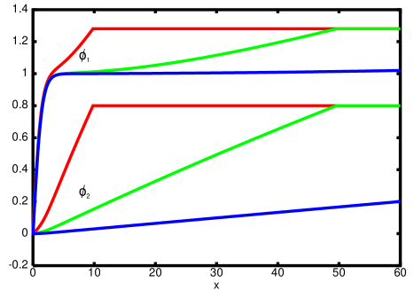
Figure 2: This figure shows the fields for the restricted kinks for different values of $R_{\infty}$. The values of $R_{\infty}$ are $R_{\infty}=10$, $R_{\infty}=50$ and $R_{\infty}=250$. The boundary conditions on $\phi_{2}$ are $\phi_{2}(\pm R_{\infty})=\pm 0.8$. The fields for negative values of $x$ just follow from symmetry of the configuration and are not plotted. This figure clearly shows the separation of the solution in the kink and a tail in the limit of small $z_{\pm}/R_{\infty}$.

Using these approximate restricted kink solutions we can also determine the position of the kink with respect to the boundaries of the space. We can get an estimate by minimizing the energy in the tails. Both tails want to spread as much as they can to lower the energy, so if there is an asymmetry in the boundary conditions of $\phi_{2}$, this will certainly have an effect. We approximate the position of the kink by minimizing the sum of the energy of the two tails, which is given by:

$$E_{tail}=\frac{z_{+}^{2}}{R_{+}}+\frac{z_{-}^{2}}{R_{-}}\quad,$$ (5)

with $R_{+}+R_{-}=2R_{\infty}$ and $z_{\pm}$ the values of the modulus field at the boundaries of space.

Minimizing this energy under the restriction $R_{+}+R_{-}=2R_{\infty}$ gives:

$$R_{+}=\frac{2}{1+|\frac{z_{-}}{z_{+}}|}R_{\infty}\quad;\quad R_{-}=\frac{2}{1+|\frac{z_{+}}{z_{-}}|}R_{\infty}\quad,$$ (6)

with $R_{+}$ and $R_{-}$ the distance between the core of the kink and the $+R_{\infty}$ and $-R_{\infty}$ boundary of space respectively. Note that the position of the kink in this estimate does not depend on the relative sign between the boundary conditions on $\phi_{2}$ at $+R_{\infty}$ and $-R_{\infty}$. We tested this simple estimate numerically and found it to work quite well, see figure 3. It should be clear that for $R_{\pm}<R_{c}$ the estimates of $R_{+}$ and $R_{-}$ break down.

In figures 3(a) and 3(b) we plotted the numerical data for the position of the kink and the estimated position of the kink. We show the results of numerical simulations for $R_{\infty}=50$, where we defined the position of the kink by the zero of the $\phi_{1}$ field. The boundary conditions we put on $\phi_{2}$ are $\phi_{2}(R_{\infty})=2+\delta$ and $\phi_{2}(-R_{\infty})=\pm 2\mp\delta$, with $\delta$ running from zero to two. In figure 3(a) we plotted $R_{-}$ as a function of $z_{+}/z_{-}$, where in 3(b) we plotted $R_{-}$ as a function of $\delta$. The plots show a good agreement between the estimate and the numerical data we obtained. They also show the independence of the position of the kink on the sign of $z_{-}/z_{+}$, which is equal to the sign of $\phi_{2}(-R_{\infty})/\phi_{2}(+R_{\infty})$.

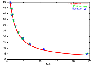
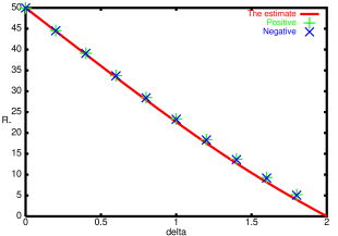
(a) (b)

Figure 3:
The figures (a) and (b) show the estimate for $R_{-}$ and the numerically obtained values of $R_{-}$ as a function of $z_{+}/z_{-}$, figure (a), and of $\delta$, figure (b), with $R_{\infty}=50$. The boundary values of $\phi_{2}$ are $\phi_{2}(R_{\infty})=2+\delta$ and $\phi_{2}(-R_{\infty})=\pm 2\mp\delta$. The figures show that the estimate of the position of the kink works very well and that the position of the kink is independent of the sign of $\phi_{2}(-R_{\infty})/\phi_{2}(+R_{\infty})$ as prescribed by our estimate.

In the limit of small $z_{\pm}/R_{\infty}$ we have a good understanding of the static kink solution. In the next section we will study the dynamics of the non static kink solutions, which occur if the boundary values of the $\phi_{2}$ field are not zero.

2.4 Non static kink configurations

In section 2.2 we proved that in an infinite space there is only a static kink solution to the field equations for a specific set of boundary values of $\phi_{2}$, notably $\phi_{2}(\pm\infty)=0$. In any other case there is no static kink solution to the equations of motion. In this section we will investigate the behavior of these non static kinks and find the DVS.
The modulus field $z$ obeys the free massless equation of motion, which in one dimension is given by:

$$-\partial_{t}^{2}z(x,t)+\partial_{x}^{2}z(x,t)=0\quad.$$ (7)

Thus the modulus field is given by $z(x,t)=z_{r}(t-x)+z_{l}(t+x)$. This shows that the modulus field propagates with the speed of light. Next we will look at some specific dynamical simulations. In the light of the previous discussion of constrained kinks it is clear what should happen in an infinite space. The kink will ’eject’ a so called scalar cloud, the tail, to infinity; the cloud will move with the speed of light, and will dynamically select the vacuum with $\phi_{2}=0$.

We look at two types of initial configurations. One corresponds with the solution of a restricted kink, which we numerically determined in the previous section. The other initial configuration is a configuration with constant $\phi_{2}$ and for $\phi_{1}$ the static kink solution with $f^{2}$ replaced by $f^{2}+\phi_{2}^{2}$, see equation (8). Both types of initial configurations we assume to be at rest at $t=0$.

Lets us first examine the latter case. Again in our numerical simulations we take $\lambda=f=1$, and start with:

$$\phi_{2}(x)=\phi_{2}\quad;\quad\phi_{1}(x)=\sqrt{1+\phi_{2}^{2}}\tanh(\frac{1}{2}\sqrt{2}\sqrt{1+\phi_{2}^{2}}~{}x),$$ (8)

taking $\partial_{t}\phi_{1}(t)|_{t=0}=\partial_{t}\phi_{2}(t)|_{t=0}=0$. As expected, we find that the scalar cloud moves away with the speed of light and the special vacuum with $\phi_{2}=0$ is dynamically selected, see figure 4(a).

The initial condition with the restricted kink as the initial configuration yields a similar result. We determined the solution of the restricted kink, with $R_{\infty}=50$ and $\phi_{2}(\pm R_{\infty})=0.8$, with the help of a relaxation program and used it as the initial configuration of the dynamical process. Again we take $\partial_{t}\phi_{2}(t)|_{t=0}=\partial_{t}\phi_{1}(t)|_{t=0}=0$. Also here the special vacuum with $\phi_{2}=0$ is dynamically selected, see figure 4(b).

After the vacuum has been selected the kink can still be excited, which is clear in the first case, equation (8). In the case where the restricted kink has been chosen as initial configuration, the kink is only slightly excited locally, due to the overlap of the kink and the modulus field. We conclude that this part of the dynamics depends on the initial condition, but does not effect the vacuum selection part of the dynamics.

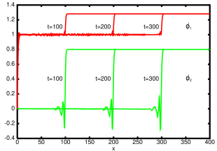
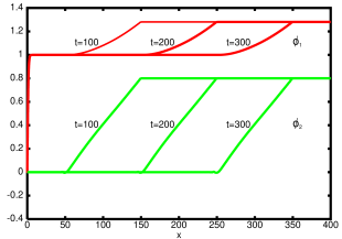
(a) (b)

Figure 4:
(a):The dynamics of the kink with $\phi_{2}(x)=\phi_{2}=0.8$ and $\phi_{1}(x)$ given by equation (8) at $t=0$. The figure shows snapshots of the fields $\phi_{1}(x)$ and $\phi_{2}(x)$ at $t=100$, $t=200$ and $t=300$. This shows the DVS and the speed of the scalar cloud.
(b):The dynamics of the restricted kink with $\phi_{2}(\pm R_{\infty})=0.8$ and $R_{\infty}=50$ at $t=0$. The figure shows snapshots of the fields $\phi_{1}(x)$ and $\phi_{2}(x)$ at $t=100$, $t=200$ and $t=300$. This shows the DVS and the speed of the scalar cloud.
The values of the fields for negative values of $x$ follow from symmetry of the configuration and are not plotted.

3 DVS in 2 dimensions

In this section we briefly recall known results of DVS in two dimensions, as discussed in [2]. Witten in [1] already observed, that in several models not all boundary conditions allow for static vortex solutions. In the model, studied in [2] there is also a potential of the form $\frac{\lambda}{4}(|\phi_{1}|^{2}-|\phi_{2}|^{2}-f^{2})^{2}$. The Higgs fields they use are now complex scalar fields, oppositely charged under a local $U(1)$. Also in this model the vacuum $\phi_{2}=0$ is dynamically selected in a topologically nontrivial sector of the theory. In [5] it was pointed out that this specific vacuum was selected as to minimize the mass of the massive gauge boson.

Again the main idea behind the DVS is the fact that one can make a tail with the modulus field, which brings fields from one point of the vacuum manifold to an other point in the same connected component of the vacuum manifold. In two dimensions the energy cost of such a tail is inversely proportional to $\ln{\frac{R_{\infty}}{R_{c}}}$ and can be made arbitrarily small in an infinite space. Although the dynamics of the modulus field is a bit different in two dimensions from the dynamics in one dimension, the conclusion is the same: DVS takes place. For more details on DVS in two dimensions we refer to [1], [2] and [5].

4 No DVS in 3 dimensions

To conclude we look at a specific model in three dimensions to argue that DVS does not work in three dimensions (as was already mentioned in [2]). The crucial observation here is that a tail in which the modulus field connects one point of the vacuum manifold to another point in the same connected component, will cost a finite amount of energy. In three dimensions the energy of such a modulus field is proportional to $\frac{R_{c}R_{\infty}}{R_{\infty}-R_{c}}$, which does not go to zero in the limit of $R_{\infty}\to\infty$, suggesting that there is no DVS in three dimensions.

To make this more explicit we discuss a model which has a local $SU(2)$ symmetry and two scalar Higgs fields in the vector representation of the local gauge group. The potential will again have the form $\frac{\lambda}{4}(Tr\{\phi_{1}^{2}\}-Tr\{\phi_{2}^{2}\}-f^{2})^{2}$. In this model the $SU(2)$ gauge symmetry is spontaneously broken to $U(1)$ and topologically stable magnetic monopoles can form. The action of the model is given by:

$$S=\int d^{4}x\{\frac{1}{4}F_{\mu\nu}^{a}F^{a,\mu\nu}+\frac{1}{2}Tr\{(D_{\mu}\phi_{1})^{2}\}+\frac{1}{2}Tr\{(D_{\mu}\phi_{2})^{2}\}-\frac{\lambda}{4}(Tr\{\phi_{1}^{2}\}-Tr\{\phi_{2}^{2}\}-f^{2})^{2}\}\quad.$$ (9)

We will try to find static monopole solutions in the BPS limit, i.e., we keep the boundary terms fixed but put $\lambda$ to zero. We note that the fields $\phi_{1}$ and $\phi_{2}$ need to be parallel to each other in the internal space at spatial infinity in order to have a finite energy solution, and to have an unbroken $U(1)$ in the first place. We will focus on static configurations where $Tr\{\phi_{2}(r\to\infty)^{2}\}$ does not depend on the spatial angles.

To find static solutions we have to extremize the energy:

$$E=\int d^{3}x\{\frac{1}{2}B^{2}+\frac{1}{2}Tr\{(D_{i}\phi_{1})^{2}\}+\frac{1}{2}Tr\{(D_{i}\phi_{2})^{2}\}\}\quad.$$ (10)

To be able to get the BPS equations we first make the following rescalings: $\phi_{1}\to\cosh{u}~{}\phi_{1}$,$\phi_{2}\to\sinh{u}~{}\phi_{2}$, $x_{i}\to\frac{1}{\sqrt{\cosh{2u}}}~{}x_{i}$ and $A_{i}\to\sqrt{\cosh{2u}}~{}A_{i}$, where $Tr\{\phi_{2}(\infty)^{2}\}=\sinh^{2}{u}$. Note the similarity with the usual BPS dyon. Now we can write the energy in the following form:

$$E=\frac{1}{\sqrt{\cosh{2u}}}\int d^{3}x\{\cosh^{2}{u}~{}(\frac{1}{2}B^{2}+\frac{1}{2}Tr\{(D_{i}\phi_{1})^{2}\})+\sinh^{2}{u}~{}(\frac{1}{2}B^{2}+\frac{1}{2}Tr\{(D_{i}\phi_{2})^{2}\})\}\quad.$$ (11)

From this we get the usual BPS equations for the monopole twice, one for $\phi_{1}$ and one for $\phi_{2}$. They reduce to one set of BPS equations under the assumption $\phi_{1}=\phi_{2}$, whose solution is well known. The energy of the monopole is simply given by:

$$E_{mon}=\sqrt{\cosh{2u}}~{}E_{mon;~{}u=0}\quad,$$ (12)

where $E_{mon;~{}u=0}$ is the energy of the monopole in absence of $\phi_{2}$.
This shows that the core structure of the monopole is effected by the boundary conditions of the $\phi_{2}$ field and that there is no DVS. This in contrast with the results found in one and two dimensions.

5 Conclusion and outlook

In this paper we showed the possibility of dynamical vacuum selection (DVS) in one dimensional field theories with flat directions. We examined this DVS with the help of a specific model. For this model we proved that there is only one specific boundary condition which allows a static kink solution in an infinite space. In a finite space any boundary condition allows the formation of a static kink. With the help of a relaxation program we numerically determined these restricted kinks. They can be very well described by one specific kink with a scalar cloud on each side of the kink. This description of the restricted kink also correctly predicts the position of the kink with respect to the boundaries of the space as a function of the boundary conditions. Using a numerical simulation we examined the dynamical properties of configurations with boundary conditions which do not allow a static solution in an infinite space. These simulations confirm the DVS, which was expected to occur, from the result of the restricted kinks and the field equation for the modulus field.

It should be clear that DVS in one dimension is not specific for the one dimensional model we considered. It is a general feature of one dimensional models with flat directions. The argument relies crucially on the the scaling of the energy of the tails, the scalar clouds, of the restricted kinks. In these scalar clouds only the modulus field changes. More generally this shows that DVS is only possible in one and, as was shown before [2], in two dimensions, but not in three or higher dimensions. For completeness we briefly mentioned the two dimensional case and included an explicit example of a three dimensional model where DVS does not work.

It remains of course possible that a model has more then one possible static configuration in an infinite space [6], but the DVS will just pick out one of the possible static solitons and including tunneling it will eventually always select the vacuum corresponding to the static soliton with the lowest energy. Although this DVS selects a lowest energy static soliton solution there can still be a vacuum and core degeneracy left if the groundstate of the topologically non trivial sector is degenerate, as was for example found in [5].

It would be interesting to study DVS, due to the presence of a soliton, in a theory where the selected vacuum is lifted from the classical vacuum manifold by quantum mechanical (or thermal) corrections. Obviously this cannot happen if a supersymmetric BPS soliton is selected by the DVS, since the energy of such a BPS soliton is protected against quantum mechanical corrections. On the length scale where the quantum mechanical corrections to the vacuum manifold would become important the DVS alters and most likely a type of restricted soliton will become the new selected vacuum. The tail(s) of these restricted solitons will presumably have a length of the order determined by the quantum mechanical corrections to the classical vacuum manifold.
We would like to thank A. Achúcarro, L. Pogosian and T. Vachaspati for discussions. One of us (J.S.) thanks the ESF, COSLAB program, for supporting the participation in the COSLAB 2002 workshop.

References

- [1] Edward Witten. Phases of N=2 theories in two dimensions. Nucl. Phys., B403:159–222, 1993.
- [2] A. A. Penin, V. A. Rubakov, P. G. Tinyakov, and S. V. Troitsky. What becomes of vortices in theories with flat directions. Phys. Lett., B389:13–17, 1996.
- [3] E. B. Bogomolny. Stability of classical solutions. Sov. J. Nucl. Phys., 24:449, 1976.
- [4] Ian Affleck. On constrained instantons. Nucl. Phys., B191:429, 1981.
- [5] A. Achúcarro, A. C. Davis, M. Pickles, and J. Urrestilla. Vortices in theories with flat directions. Phys. Rev., D66:105013, 2002.
- [6] Levon Pogosian and Tanmay Vachaspati. Space of kink solutions in SU(n) x Z(2). Phys. Rev., D64:105023, 2001.