Abstract

We use matrix model technology to study the $\mathcal{N}=2$ $\mathrm{U}(N)$ gauge theory with $N_{f}$ massive hypermultiplets in the fundamental representation. We perform a completely perturbative calculation of the periods $a_{i}$ and the prepotential $\mathcal{F}(a)$ up to the first instanton level, finding agreement with previous results in the literature. We also derive the Seiberg-Witten curve and differential from the large-$M$ solution of the matrix model. We show that the two cases $N_{f}<N$ and $N\leq N_{f}<2N$ can be treated simultaneously.

1 Introduction

Dijkgraaf, Vafa, and collaborators have discovered remarkable relations between perturbative matrix models and instanton effects in supersymmetric gauge theories [1]–[4]. Recently we used the new matrix model technology to study the $\mathcal{N}=2$ $\mathrm{U}(N)$ gauge theory [5] (ref. [5] also contains a more extensive list of references). We calculated the prepotential $\mathcal{F}(a)$ and the periods $a_{i}$ perturbatively up to the first instanton level. A new ingredient in our calculation was a completely perturbative definition of the periods $a_{i}$ as functions of the classical moduli $e_{i}$. Our results combined with those of Dijkgraaf and Vafa show that, even when the matrix model cannot be completely solved, a perturbative diagrammatic expansion of the matrix model can still be used to obtain all the low-energy non-perturbative information of $\mathcal{N}=2$ gauge theories order-by-order in the instanton expansion.

In this paper we study the $\mathcal{N}=2$ U($N$) gauge theory with $N_{f}$ hypermultiplets transforming in the fundamental representation of the gauge group using matrix model techniques. Several new features present themselves in this case, making the model well worth studying.

In the first part of the paper, we extend the perturbative results obtained in [5] for the $\mathcal{N}=2$ $\mathrm{U}(N)$ theory to the case with $N_{f}$ fundamental matter hypermultiplets. A new feature of the calculation, compared to the one in [5], is the appearance of planar diagrams with boundaries [6]. These contribute, in the diagrammatic expansion of the matrix model, to the free energy and superpotential. They also affect the relation between the periods $a_{i}$ and the classical moduli $e_{i}$. We compute the periods $a_{i}$ and prepotential $\mathcal{F}(a)$ perturbatively to first order in the instanton expansion, finding agreement with earlier results in the literature. This agreement is a test of our proposed relation [5] between $a_{i}$ and $e_{i}$.

In the case of U($N$) with fundamental matter, there is an ambiguity in the form of the Seiberg-Witten curve [7] for $N\leq N_{f}<2N$ [8]–[10], with different forms of the curve corresponding to different definitions of the classical moduli $e_{i}$. These different curves yield slightly different relations between $a_{i}$ and $e_{i}$. Our perturbative calculation, which does not start from a curve, yields an unambiguous relation between $a_{i}$ and $e_{i}$ and therefore implies a particular form the of the Seiberg-Witten curve, which we show to be $y^{2}=\prod_{i=1}^{N}(x-e_{i})^{2}-f_{N-1}(x)$ where $f_{N-1}(x)$ is an $(N-1)$th order polynomial specified in eq. (6).

In the second part of the paper we derive the form of the Seiberg-Witten curve and differential for the $\mathcal{N}=2$ $\mathrm{U}(N)$ gauge theory with $N_{f}$ fundamental hypermultiplets, from the large-$M$ saddle-point solution to the matrix model, without any additional input. The result is consistent with known results [7]–[10] and also agrees with the form of the curve implied by the perturbative calculation. Our results give further support to the idea that all the low-energy information about the $\mathcal{N}=2$ theory is contained in the matrix model. (Very recently some aspects of the relation between matrix models and Seiberg-Witten theory have been discussed in ref. [12].)

An important question is why the matrix model approach to supersymmetric gauge theories works and what the scope and limitations of the method are. Recently, these questions have been explored and purely field-theoretic proofs for the correctness of the matrix model approach have been presented for the pure $\mathcal{N}=1$ $\mathrm{U}(N)$ gauge theory with an arbitrary polynomial superpotential [13, 14]. It would be interesting to extend these results to cover the model studied in this paper. Also, ref. [15] discusses some aspects of the correspondence between matrix-model and gauge-theory quantities.

In sec. 2 we set up the perturbative calculation. In sec. 3 we calculate $\tau_{ij}$ as a function of the classical moduli to first order in the instanton expansion. In sec. 4 we extend our proposed perturbative definition of the periods $a_{i}$ to the case when fundamentals are present, and use this result to determine the one-instanton corrections to $a_{i}$. In sec. 5 we compute the one-instanton correction to the prepotential $\mathcal{F}(a)$. When $N_{f}\geq N$ a certain polynomial appears in the relation between $a_{i}$ and the classical moduli; the role of this polynomial is clarified in sec. 6. In sec. 7 we derive the Seiberg-Witten curve from the large-$M$ saddle point solution to the matrix model. In sec. 8 we derive the Seiberg-Witten differential from within the matrix model framework. We conclude the paper with a summary of our findings.

2 Perturbative matrix model approach

In this section, we describe the perturbative matrix model approach to the $\mathcal{N}=2$ $\mathrm{U}(N)$ gauge theory with matter in the fundamental representation, extending our earlier work [5]. Previous work discussing matter in the fundamental representation (focusing mainly on $\mathcal{N}=1$ theories) in the matrix model context can be found in [6] [16]–[20].

In the presence of (massless or massive) $\mathcal{N}=2$ hypermultiplets transforming in the fundamental representation, the $\mathcal{N}=2$ $\mathrm{U}(N)$ gauge theory develops a superpotential

$$W_{\mathrm{mat}}(\phi,q,\tilde{q})=\sum_{I=1}^{N_{f}}\left[\tilde{q}_{I}\phi\,q^{I}+m_{I}\tilde{q}_{I}q^{I}\right]\,,$$ (2.1)

written in terms of the $\mathcal{N}=1$ fields $\phi$ (the adjoint scalar in the $\mathcal{N}=2$ vector multiplet), $q^{I}$ ($I=1,\ldots N_{f}$) transforming in the fundamental representation and $\tilde{q}_{I}$, transforming in the conjugate fundamental representation. We have suppressed the gauge group indices, and $m_{I}$ are the masses of the fundamentals.

The first step of the matrix model program is to break $\mathcal{N}=2$ supersymmetry to $\mathcal{N}=1$ by adding a tree-level superpotential $W_{0}(\phi)$ to the gauge theory. The particular choice of $W_{0}(\phi)$ relevant to us is the one that freezes the moduli to a generic point on the Coulomb branch of the $\mathcal{N}=2$ theory:

$$W_{0}(\phi)=\alpha\sum_{\ell=0}^{N}{s_{N-\ell}(e)\over\ell{+}1}{\rm tr}(\phi^{\ell+1})\quad\Rightarrow\quad W^{\prime}_{0}(x)=\alpha\prod_{i=1}^{N}(x-e_{i})\,,$$ (2.2)

where $e_{i}$ are the classical moduli, $s_{m}(e)$ is the elementary symmetric polynomial

$$s_{m}(e)=(-1)^{m}\sum_{i_{1}<i_{2}<\cdots<i_{m}}e_{i_{1}}e_{i_{2}}\cdots e_{i_{m}}\,,\qquad\qquad s_{0}=1\,,$$ (2.3)

and $\alpha$ is a parameter that will be taken to zero at the end of the calculation, restoring $\mathcal{N}\!=2$ supersymmetry [21].

The next step is to reinterpret the superpotential $W(\phi,q,\tilde{q})=W_{0}(\phi)+W_{\mathrm{mat}}(\phi,q,\tilde{q})$ as the potential of a chiral matrix model [1]-[4], which has the partition function (denoting the matrix model analogs of $\phi$, $q$, and $\tilde{q}$ with capital letters)

$$Z={1\over\mathrm{vol}(G)}\int{\rm d}\Phi\,{\rm d}Q^{I}{\rm d}\tilde{Q}_{I}\exp\left(-\frac{W(\Phi,Q,\tilde{Q})}{g_{s}}\right)\,,$$ (2.4)

where the integral is over $M{\times}M$ matrices $\Phi$ (which can be taken to be hermitian) and $M$-dimensional vectors $Q^{I}$ and $\tilde{Q}_{I}$. In eq. (2.4), $G$ is the unbroken matrix model gauge group, and $g_{s}$ is a parameter that later will be taken to zero as $M\to\infty$. In taking the $M\to\infty$ limit, we keep $N_{f}$ finite (as in ref. [18]); our approach thus differs from the one in [16]. The matrix integral (2.4) is evaluated perturbatively about an extremal point $\Phi=\Phi_{0}$, $Q_{0}=0$, $\tilde{Q}_{0}=0$ of $W(\Phi,Q,\tilde{Q})$. We write

$$\Phi=\Phi_{0}+\Psi=\pmatrix{e_{1}1\kern-3.0pt\mathrm{l}_{M_{1}}&0&\cdots&0\cr 0&e_{2}1\kern-3.0pt\mathrm{l}_{M_{2}}&\cdots&0\cr\vdots&\vdots&\ddots&\vdots\cr 0&0&\cdots&e_{N}1\kern-3.0pt\mathrm{l}_{M_{N}}}+\pmatrix{\Psi_{11}&\Psi_{12}&\cdots&\Psi_{1N}\cr\Psi_{21}&\Psi_{22}&\cdots&\Psi_{2N}\cr\vdots&\vdots&\ddots&\vdots\cr\Psi_{N1}&\Psi_{N2}&\cdots&\Psi_{NN}}\,,$$ (2.5)

where $\sum_{i}M_{i}=M$, and $\Psi_{ij}$ is an $M_{i}\,{\times}M_{j}$ matrix. This choice breaks the $\mathrm{U}(M)$ symmetry to $G=\prod_{i=1}^{N}U(M_{i})$.

The connected diagrams of the perturbative expansion of $Z$ may be organized, using the standard double-line notation, in a topological expansion characterized by the Euler characteristic $\chi$ of the surface in which the diagram is embedded [22]

$$Z=\exp\left(\sum_{\chi\leq 2}g_{s}^{-\chi}F_{\chi}(e,S)\right)\quad{\rm where~{}}\quad S_{i}\equiv g_{s}M_{i}\,,$$ (2.6)

where $\chi=2{-}2g{-}h$ with $g$ the genus (number of handles) and $h$ the number of holes. When evaluating the matrix integral in the $M_{i}\to\infty$, $g_{s}\to 0$ limit, with $S_{i}$ held fixed, the leading contribution comes from the planar diagrams that can be drawn on the sphere ($\chi=2$),

$$F_{\rm s}(e,S)\equiv F_{\chi=2}(e,S)=g_{s}^{2}\log Z\bigg{|}_{\rm sphere}$$ (2.7)

As discussed in [6], the presence of the $Q^{I}$, $\tilde{Q}_{I}$’s leads to the introduction of surfaces with boundaries in the topological expansion. The leading boundary contribution comes from surfaces with one boundary (disks), obtained from the sphere by cutting out one hole, and having $\chi=1$,

$$F_{\rm d}(e,S)\equiv F_{\chi=1}(e,S)=g_{s}\log Z\bigg{|}_{\rm disk}$$ (2.8)

It was shown in [5] (generalizing the result in [4] for $\mathrm{U}(2)$) that when one expands $W_{0}(\Phi)$ (2.2) to quadratic order in $\Psi$, the coefficients of ${\rm tr}(\Psi_{ij}\Psi_{ji})$ vanish when $i{\neq}j$. Hence the off-diagonal matrices $\Psi_{ij}$ are zero modes, and correspond to pure gauge degrees of freedom. As in ref. [4, 5], we fix the gauge $\Psi_{ij}=0$ ($i{\neq}j$) and introduce Grassmann-odd ghost matrices $B$ and $C$ with action

$${\rm tr}\left(B[\Phi,C]\right)=\sum_{i=1}^{N}\sum_{j\neq i}(e_{i}-e_{j}){\rm tr}(B_{ji}C_{ij})+\sum_{i=1}^{N}\sum_{j\neq i}{\rm tr}(B_{ji}\Psi_{ii}C_{ij}-B_{ji}C_{ij}\Psi_{jj})\,.$$ (2.9)

In the $\Psi_{ij}=0$ ($i{\neq}j$) gauge $W_{0}(\Phi)$ becomes [5]

$$W_{0}(\Phi)=\sum_{i=1}^{N}M_{i}W_{0}(e_{i})+{\alpha}\sum_{i=1}^{N}{R_{i}\over 2}{\rm tr}(\Psi_{ii}^{2})+{\alpha}\sum_{i=1}^{N}\sum_{p=3}^{N}{\gamma_{p,i}\over p}{\rm tr}(\Psi_{ii}^{p})\,,$$ (2.10)

where $R_{i}=\prod_{j\neq i}e_{ij}$ with $e_{ij}=e_{i}-e_{j}$, and

$$\gamma_{p,i}={1\over(p-1)!}\left[\left(\partial\over\partial x\right)^{p-1}\prod_{k=1}^{N}(x-e_{k})\right]\Bigg{|}_{x=e_{i}}$$ (2.11)

Writing $Q^{I}=(Q^{I}_{1},Q_{2}^{I},...,Q_{N}^{I})^{T}$, where $Q^{I}_{i}$ is an $M_{i}$-dimensional vector and similarly for $\tilde{Q}_{I}$, and expanding $W_{\rm mat}(\Phi,Q^{I},\tilde{Q}_{I})$ around the vacuum (2.5) one finds (using the $\Psi_{ij}=0$ ($i{\neq}j$) gauge)

$$W_{\mathrm{mat}}(\Phi,Q,\tilde{Q})=\sum_{i=1}^{N}\sum_{I=1}^{N_{f}}\left[(e_{i}+m_{I})\tilde{Q}_{iI}Q_{i}^{I}+\tilde{Q}_{iI}\Psi_{ii}Q_{i}^{I}\right]\,.$$ (2.12)

Collecting the above results, the partition function is given by the gauge-fixed integral

$$Z_{\rm g.f.}={1\over\mathrm{vol}(G)}\exp\left(-{1\over g_{s}}\sum_{i=1}^{N}M_{i}W_{0}(e_{i})\right)\int{\rm d}\Psi_{ii}\,{\rm d}B_{ij}\,{\rm d}C_{ij}\,{\rm d}Q^{I}{\rm d}\tilde{Q}_{I}{\rm e}^{I_{\rm quad}+I_{\rm int}}$$ (2.13)

where the quadratic part of the action is

$$I_{\rm quad}=-{\alpha\over g_{s}}\sum_{i=1}^{N}{R_{i}\over 2}{\rm tr}(\Psi_{ii}^{2})-\sum_{i=1}^{N}\sum_{j\neq i}e_{ij}{\rm tr}(B_{ji}C_{ij})-{1\over g_{s}}\sum_{i=1}^{N}\sum_{I=1}^{N_{f}}(e_{i}+m_{I})\tilde{Q}_{iI}Q_{i}^{I}\,,$$ (2.14)

and the interaction terms are

$$I_{\rm int}=-{\alpha\over g_{s}}\sum_{i=1}^{N}\sum_{p=3}^{N}{\gamma_{p,i}\over p}{\rm tr}(\Psi_{ii}^{p})-\sum_{i=1}^{N}\sum_{j\neq i}{\rm tr}(B_{ji}\Psi_{ii}C_{ij}-B_{ji}C_{ij}\Psi_{jj})-{1\over g_{s}}\sum_{i=1}^{N}\sum_{I=1}^{N_{f}}\tilde{Q}_{iI}\Psi_{ii}Q_{i}^{I}\,.$$ (2.15)

The propagators for the various fields can be read off from eq. (2.14) and the vertices from eq. (2.15). Each ghost loop will acquire an additional factor of $(-2)$ [4].

3 Perturbative calculation of $\tau_{ij}(e)$

The integral over the part of the quadratic action (2.14) involving $\Psi_{ii}$, $B_{ij}$, and $C_{ij}$ can be explicitly performed [5]; including also the classical piece one finds (up to an $e_{i}$-independent quadratic monomial in the $S_{i}$’s)

$$F_{\rm s}(e,S)=-\sum_{i=1}^{N}S_{i}W_{0}(e_{i})+{\textstyle\frac{1}{2}}\sum_{i=1}^{N}S_{i}^{2}\log\left(S_{i}\over\alpha R_{i}\hat{\Lambda}^{2}\right)+\sum_{i=1}^{N}\sum_{j\neq i}S_{i}S_{j}\log\left(e_{ij}\over\hat{\Lambda}\right)+\sum_{n\geq 3}F^{(n)}_{\rm s}(e,S)$$ (3.1)

As in [4], we have included in eq. (3.1) a contribution $-\left(\sum_{i=1}^{N}S_{i}\right)^{2}\log\hat{\Lambda}$ that reflects the ambiguity in the cut-off of the full $\mathrm{U}(M)$ gauge group. (A similar contribution is included in (3.4) below.) The term $F^{(n)}_{\rm s}(e,S)$ is an $n$th order polynomial in $S_{i}$ arising from planar loop diagrams built from the interaction vertices [3]. The contribution to $F_{\rm s}(e,S)$ cubic in $S_{i}$ was computed in [5] with the result:

$$\alpha F^{(3)}_{\rm s}(e,S) = ({\textstyle\frac{1}{2}}+{\textstyle\frac{1}{6}})\sum_{i}\frac{S_{i}^{3}}{R_{i}}\left(\sum_{k\neq i}{1\over e_{ik}}\right)^{2}-{\textstyle\frac{1}{4}}\sum_{i}\frac{S_{i}^{3}}{R_{i}}\sum_{k\neq i}\sum_{\ell\neq i,k}{1\over e_{ik}e_{i\ell}}$$ (3.2)

$$-2\sum_{i}\sum_{k\neq i}\frac{S_{i}^{2}S_{k}}{R_{i}e_{ik}}\sum_{\ell\neq i}\frac{1}{e_{i\ell}}+2\sum_{i}\sum_{k\neq i}\sum_{\ell\neq i}\frac{S_{i}S_{k}S_{\ell}}{R_{i}e_{ik}e_{i\ell}}-\sum_{i}\sum_{k\neq i}\frac{S_{i}^{2}S_{k}}{R_{i}e_{ik}^{2}}\,.$$

Next we turn to the contribution of the fundamentals $Q$, $\tilde{Q}$ to the matrix model free energy. Since these involve quark loops, they only contribute to the disk-level part of the free energy. The integral over the quadratic part of $W_{\mathrm{mat}}$ gives

$$\int\prod_{i=1}^{N}\prod_{I=1}^{N_{f}}{\rm d}Q^{I}_{i}{\rm d}\tilde{Q}_{iI}\exp\left(-\frac{1}{g_{s}}(e_{i}+m_{I})\tilde{Q}_{iI}Q_{i}^{I}\right)=\exp\left(-\sum_{i=1}^{N}\sum_{I=1}^{N_{f}}M_{i}\log\frac{(e_{i}+m_{I})}{g_{s}}\right)$$ (3.3)

which yields (up to an $e_{i}$-independent part linear in $S_{i}$) the first term of

$$F_{\rm d}(e,S)=-\,\sum_{i=1}^{N}\sum_{I=1}^{N_{f}}S_{i}\log\frac{(e_{i}+m_{I})}{\hat{\Lambda}}+\sum_{n\geq 2}F^{(n)}_{\rm d}(e,S)$$ (3.4)

Here $F^{(n)}_{\rm d}(e,S)$ is an $n$th order polynomial in $S_{i}$ arising from planar disk diagrams built from the interaction vertices. To obtain the $\mathcal{O}(S^{2})$ contribution to $F_{\rm d}(e,S)$, we need to evaluate the diagrams displayed in figure 1.

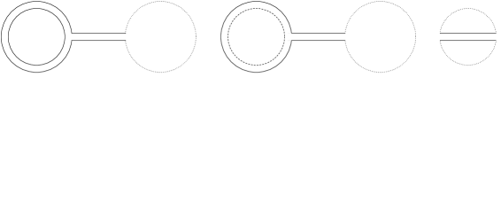
Figure 1: Disk diagrams contributing to $F_{\rm d}(e,S)$ at order $\mathcal{O}(S^{2})$. Solid double lines refer to $\Psi_{ii}$ propagators, solid-plus-dashed double lines refer to ghost propagators, and single dotted lines correspond to the propagator for the $Q$’s.

One might also consider diagrams drawn on surfaces with additional holes. One example is a “dumb-bell” diagram as in figure 1, but with quark propagators at both ends. Such a diagram corresponds to a sphere with two holes, the dotted lines encircling each of the two holes. However, such a surface has $\chi=0$ and the diagram is therefore suppressed by a factor of $g_{s}$ relative to the $\chi=1$ disk contribution in the $g_{s}\rightarrow 0$, $M_{i}\rightarrow\infty$ limit.

The above diagrams lead to:

$$\alpha F^{(2)}_{\rm d}(e,S)=\sum_{I=1}^{N_{f}}\left[\sum_{i}{S^{2}_{i}\over R_{i}f_{iI}}\sum_{j\neq i}\frac{1}{e_{ij}}-2\sum_{i}\sum_{j\neq i}\frac{S_{i}S_{j}}{R_{i}e_{ij}f_{iI}}+{\textstyle\frac{1}{2}}\sum_{i}\frac{S^{2}_{i}}{R_{i}f_{iI}^{2}}\right]\,,$$ (3.5)

where $f_{iI}=e_{i}+m_{I}$.

To relate the matrix model and its free energy to the $\mathcal{N}=2$ U($N$) gauge theory (with $N_{f}$ hypermultiplets in the fundamental representation of the gauge group) broken to $\prod_{i}\mathrm{U}(N_{i})$, one introduces [1]–[3] [24] [6]

$$W_{\rm eff}(e,S)=-\sum_{i=1}^{N}N_{i}{\partial F_{\rm s}(e,S)\over\partial S_{i}}-F_{\rm d}(e,S)+2\pi i\tau_{0}\sum_{i=1}^{N}S_{i}\,,$$ (3.6)

where $\tau_{0}=\tau(\Lambda_{0})$ is the gauge coupling of the U$(N)$ theory at some scale $\Lambda_{0}$. Since we are breaking $\mathrm{U}(N)$ to $\mathrm{U}(1)^{N}$, we set $N_{i}=1$ for $i=1,\ldots,N$. It was conjectured in ref. [6] that the disk-level part of the free energy $F_{\rm d}(e,S)$ contributes to $W_{\rm eff}$ without any derivatives acting on it. We will find further support for this claim. Next, one extremizes the effective superpotential with respect to $S_{i}$ to obtain $\langle{S_{i}}\rangle$:

$${\partial W_{\rm eff}(e,S)\over\partial S_{i}}\bigg{|}_{S_{j}=\langle{S_{j}}\rangle}=0\,.$$ (3.7)

Finally,

$$\tau_{ij}(e)={1\over 2\pi i}{\partial^{2}F_{\rm s}(e,S)\over\partial S_{i}\partial S_{j}}\bigg{|}_{S_{i}=\langle{S_{i}}\rangle}$$ (3.8)

yields the couplings of the unbroken U$(1)^{N}$ factors of the gauge theory, as a function of $e_{i}$. Note that although both the Seiberg-Witten formula $\tau_{ij}(a)=\frac{\partial^{2}\mathcal{F}(a)}{\partial a_{i}\partial a_{j}}$ and (3.8) refer to the same quantity (the period matrix of the Seiberg-Witten curve $\Sigma$), they are expressed in terms of different parameters on the moduli space ($a_{i}$ vs. $e_{i}$).

Above, we have evaluated $F_{\rm s}(e,S)$ to cubic order in $S_{i}$ and $F_{\rm d}(e,S)$ to quadratic order in $S_{i}$, which will be sufficient to obtain $\tau_{ij}(e)$ to one-instanton accuracy. Inserting the results eq. (3.1), (3.2), (3.4), and (3.5) in eq. (3.6), we obtain

$$\!\!\!\!\!\!W_{\rm eff}(e,S)=\sum_{i}W_{0}(e_{i})-\sum_{i}S_{i}\log\left(S_{i}\over\alpha R_{i}\hat{\Lambda}^{2}\right)-2\sum_{i}\sum_{k\neq i}S_{k}\log\left(e_{ik}\over\hat{\Lambda}\right)+\,\sum_{i}\sum_{I=1}^{N_{f}}S_{i}\log\left(f_{iI}\over\hat{\Lambda}\right)$$

$$-{1\over\alpha}\Bigg{[}\sum_{i}\sum_{k\neq i}\sum_{\ell\neq i,k}\left(-{3S_{i}^{2}\over 4R_{i}e_{ik}e_{i\ell}}+{2S_{k}S_{\ell}\over R_{i}e_{ik}e_{i\ell}}\right)+\sum_{i}\sum_{k\neq i}\left(-\frac{S_{i}^{2}}{R_{i}e_{ik}^{2}}-\frac{2S_{i}S_{k}}{R_{i}e_{ik}^{2}}+\frac{2S_{i}^{2}}{R_{k}e_{ik}^{2}}\right)$$

$$+\sum_{I=1}^{N_{f}}\sum_{i}\left(-{S^{2}_{i}\over R_{i}f_{iI}}\sum_{k\neq i}{1\over e_{ik}}+\sum_{k\neq i}{2S_{i}S_{k}\over R_{i}e_{ik}f_{iI}}-{S^{2}_{i}\over 2R_{i}f_{iI}^{2}}\right)\Bigg{]}+\left(2\pi i\tau_{0}+{\rm const}\right)\sum_{i}S_{i}\,.$$ (3.9)

The extrema $\langle{S_{i}}\rangle$ are obtained from (3.7), and can be evaluated in an expansion in $\Lambda$

$$\langle{S_{i}}\rangle = {\alpha L_{i}\over R_{i}}\Lambda^{2N-N_{f}}+{\alpha L_{i}\over R_{i}}\Lambda^{4N-2N_{f}}\Bigg{[}\sum_{k\neq i}\sum_{\ell\neq i,k}\left({3L_{i}\over 2R_{i}^{2}e_{ik}e_{i\ell}}+{4L_{\ell}\over R_{k}R_{\ell}e_{ik}e_{k\ell}}\right)$$ (3.10)

$$+\sum_{k\neq i}\left(\frac{2L_{i}}{R_{i}^{2}e_{ik}^{2}}-\frac{4L_{i}}{R_{i}R_{k}e_{ik}^{2}}+\frac{2L_{k}}{R_{i}R_{k}e_{ik}^{2}}+\frac{2L_{k}}{R_{k}^{2}e_{ik}^{2}}\right)-\sum_{I=1}^{N_{f}}{L_{i}\over R_{i}^{2}f_{iI}^{2}}$$

$$+\sum_{I=1}^{N_{f}}\sum_{k\neq i}\left(-{2L_{i}\over R_{i}^{2}e_{ik}f_{iI}}+{2L_{k}\over R_{i}R_{k}e_{ik}f_{iI}}-{2L_{k}\over R_{k}^{2}e_{ik}f_{kI}}\right)\Bigg{]}+\mathcal{O}(\Lambda^{6N-3N_{f}})$$

where $L_{i}=\prod_{I=1}^{N_{f}}(e_{i}+m_{I})$, and various constants as well as $\tau_{0}$ have been absorbed into a redefinition of the cut-off, $\Lambda={\rm const}\,{\times}\hat{\Lambda}\,{\rm e}^{\pi i\tau_{0}/N}$.

Although we are primarily interested in the $\mathcal{N}=2$ limit in this paper, the $\mathcal{N}=1$ effective superpotential may be easily computed by substituting eq. (3.10) into eq. (3). In the case $N_{f}\geq N$ one has to proceed with care, see [16, 18, 19] for further details.

Below we will make repeated use of the identity

$$\sum_{k\neq i}{L_{k}\over R_{k}e_{ik}}=-{L_{i}\over R_{i}}\sum_{k\neq i}{1\over e_{ik}}+\frac{L_{i}}{R_{i}}\sum_{I}{1\over f_{iI}}-\tilde{T}(e_{i})$$ (3.11)

which can be derived by taking the $z\to e_{i}$ limit of both sides of

$$\frac{\prod_{I=1}^{N_{f}}(z+m_{I})}{\prod_{k=1}^{N}(z-e_{k})}-{L_{i}\over R_{i}(z-e_{i})}=\sum_{k\neq i}{L_{k}\over R_{k}(z-e_{k})}+\tilde{T}(z)\,.$$ (3.12)

where the polynomial $\tilde{T}(z)=\sum_{k=0}^{N_{f}-N}\tilde{t}_{k}z^{N_{f}-N-k}$ is the positive part of the Laurent expansion of ${\prod_{I=1}^{N_{f}}(z+m_{I})}/{\prod_{k=1}^{N}(z-e_{k})}$ and is only non-zero when $N_{f}\geq N$. More explicitly, the coefficients $\tilde{t}_{k}$ are exactly as in eqs. (2.4) and (2.5) of ref. [25]; note that our $e_{i}$ are the same as their $\bar{a}_{i}$.

We can now evaluate

$$\tau_{ij}(e)={1\over 2\pi i}{\partial^{2}F_{\rm s}(e,S)\over\partial S_{i}\partial S_{j}}\bigg{|}_{S_{i}=\langle{S_{i}}\rangle}=\tau_{ij}^{\rm pert}(e)+\sum_{d=1}^{\infty}\Lambda^{(2N-N_{f})d}\tau_{ij}^{(d)}(e)\,.$$ (3.13)

The perturbative contribution (up to an additive constant) is

$$2\pi i\tau^{\rm pert}_{ij}(e)=\delta_{ij}\Bigg{[}-\sum_{k\neq i}\log\left(e_{ik}\over\Lambda\right)^{2}+\sum_{I=1}^{N_{f}}\log\left(f_{iI}\over\Lambda\right)\Bigg{]}+(1-\delta_{ij})\Bigg{[}\log\left(e_{ij}\over\Lambda\right)^{2}\Bigg{]}\,.$$ (3.14)

Using the identity (3.11) one obtains the one-instanton contribution

$$2\pi i\tau^{(1)}_{ij}(e)\!\! = \!\!\delta_{ij}\Bigg{[}\sum_{k\neq i}\sum_{\ell\neq i,k}\left({8L_{i}\over R_{i}^{2}e_{ik}e_{i\ell}}-{4L_{k}\over R_{k}^{2}e_{ik}e_{k\ell}}\right)+\sum_{k\neq i}\left({10L_{i}\over R_{i}^{2}e_{ik}^{2}}+{10L_{k}\over R_{k}^{2}e_{ik}^{2}}+{4\tilde{T}(e_{i})\over R_{i}e_{ik}}-{4\tilde{T}(e_{k})\over R_{k}e_{ik}}\right)$$ (3.15)

$$\;\;\;+\sum_{I=1}^{N_{f}}\left({L_{i}\over R_{i}^{2}f_{iI}^{2}}+\sum_{J\neq I}{2L_{i}\over R_{i}^{2}f_{iI}f_{iJ}}-\sum_{k\neq i}{8L_{i}\over R_{i}^{2}e_{ik}f_{iI}}+\sum_{k\neq i}{2L_{k}\over R_{k}^{2}e_{ik}f_{kI}}-{2\tilde{T}(e_{i})\over R_{i}f_{iI}}\right)\Bigg{]}$$

$$+ (1-\delta_{ij})\Bigg{[}\sum_{k\neq i,j}\left(-{8L_{i}\over R_{i}^{2}e_{ij}e_{ik}}-{8L_{j}\over R_{j}^{2}e_{ji}e_{jk}}+{4L_{k}\over R_{k}^{2}e_{ik}e_{jk}}\right)-{10L_{i}\over R_{i}^{2}e_{ij}^{2}}-{10L_{j}\over R_{j}^{2}e_{ij}^{2}}$$

$$\qquad\qquad\;\;\sum_{I=1}^{N_{f}}\left({4L_{i}\over R_{i}^{2}e_{ij}f_{iI}}+{4L_{j}\over R_{j}^{2}e_{ji}f_{jI}}\right)-{4\tilde{T}(e_{i})\over R_{i}e_{ij}}-{4\tilde{T}(e_{j})\over R_{j}e_{ji}}\Bigg{]}$$

to the gauge coupling matrix. Finally, we take the limit $\alpha\to 0$ to restore $\mathcal{N}=2$ supersymmetry, but this has no effect on $\tau_{ij}$, which is independent of $\alpha$.

4 Perturbative determination of $a_{i}$

If we are to use the matrix model results (3.14), (3.15) to determine the $\mathcal{N}=2$ prepotential $\mathcal{F}(a)$, we must first express $\tau_{ij}$ in terms of the periods $a_{i}$. In [5] we proposed a definition of $a_{i}$ within the context of the perturbation expansion of the matrix model, without referring to the Seiberg-Witten curve or differential. We argued in [5] that $a_{i}$ can be determined perturbatively via

$$a_{i}={\partial\tilde{W}^{i}_{\rm eff}(e,\langle{\tilde{S}}\rangle,\epsilon)\over\partial\epsilon}\bigg{|}_{\epsilon\to 0}$$ (4.1)

where $\tilde{W}^{i}_{\rm eff}(e,S,\epsilon)$ is the effective superpotential that one obtains by considering the matrix model with action $\tilde{W}^{i}(\Phi,Q,\tilde{Q})=W(\Phi,Q,\tilde{Q})+\epsilon\,{\rm tr}_{i}\,\Phi$. Here the trace is only over the $i$th block. For motivations for this proposal we refer the reader to [5]. In the present case, it is sufficient to consider

$$\tilde{Z}^{i} = {1\over\mathrm{vol}(G)}\int{\rm d}\Phi\exp\left(-\,{1\over g_{s}}\left[W(\Phi,Q,\tilde{Q})+\epsilon\,{\rm tr}_{i}\,\Phi\right]\right)$$ (4.2)

$$= \exp\left({1\over g_{s}^{2}}\tilde{F}^{i}_{\rm s}(e,S,\epsilon)+\frac{1}{g_{s}}\tilde{F}^{i}_{\rm d}(e,S,\epsilon)+\ldots\right)\,.$$

Writing $\tilde{F}^{i}_{\rm s}(e,S,\epsilon)=F_{\rm s}(e,S)+\epsilon\delta F^{i}_{\rm s}$ and similarly for $\tilde{F}^{i}_{\rm d}(e,S,\epsilon)$, and observing that to first order in $\epsilon$

$$\tilde{Z}^{i}=Z+{1\over\mathrm{vol}(G)}\int{\rm d}\Phi\left[-\,{\epsilon\over g_{s}}\right]{\rm tr}_{i}\,\Phi\exp\left(-\,{W(\Phi,Q,\tilde{Q})\over g_{s}}\right)\,,$$ (4.3)

one finds $\delta F^{i}_{\rm s}=-\,g_{s}\langle{{\rm tr}_{i}\,\Phi}\rangle\big{|}_{\rm sphere}$, where $\langle{{\rm tr}_{i}\,\Phi}\rangle\big{|}_{\rm sphere}$ is obtained by calculating all connected one-point functions at sphere-level in the matrix model with action $W(\Phi,Q,\tilde{Q})$. Similarly, $\delta F^{i}_{\rm d}=-\langle{{\rm tr}_{i}\,\Phi}\rangle\big{|}_{\rm disk}$ where $\langle{{\rm tr}_{i}\,\Phi}\rangle\big{|}_{\rm disk}$ is obtained by computing all connected one-point functions at disk-level.

Now the effective potential for the matrix integral (4.2) is

$$\tilde{W}^{i}_{\rm eff}(e,S,\epsilon) = -\sum_{j=1}^{N}N_{j}{\partial\tilde{F}^{i}_{\rm s}(e,S,\epsilon)\over\partial S_{j}}-\tilde{F}^{i}_{\rm d}(e,S,\epsilon)+2\pi i\tau_{0}\sum_{j=1}^{N}S_{j}$$ (4.4)

$$= W_{\rm eff}(e,S)-\epsilon\left[\sum_{j=1}^{N}N_{j}{\partial\over\partial S_{j}}\delta F^{i}_{\rm s}+\delta F^{i}_{\rm d}\right]\,.$$

Extremizing $\tilde{W}^{i}_{\rm eff}(e,S,\epsilon)$ with respect to $S$ gives $\langle{\tilde{S}_{i}}\rangle=\langle{S_{i}}\rangle+\epsilon\delta S_{i}+\mathcal{O}(\epsilon^{2})$. Substituting $\langle{\tilde{S}}\rangle$ into eq. (4.4), one obtains

$$\tilde{W}^{i}_{\rm eff}(e,\langle{\tilde{S}}\rangle,\epsilon)=W_{\rm eff}(e,\langle{S}\rangle)+\epsilon\sum_{j=1}^{N}\delta S_{j}{\partial W_{\rm eff}\over\partial S_{i}}\bigg{|}_{\langle{S}\rangle}-\epsilon\left[\sum_{j=1}^{N}N_{j}{\partial\over\partial S_{j}}\delta F^{i}_{\rm s}+\delta F^{i}_{\rm d}\right]\bigg{|}_{\langle{S}\rangle}+\mathcal{O}(\epsilon^{2})$$ (4.5)

The second term vanishes by the definition of $\langle{S}\rangle$. Finally, using eq. (4.1), one obtains

$$a_{i}=-\left[\sum_{j=1}^{N}N_{j}{\partial\over\partial S_{j}}\delta F^{i}_{\rm s}+\delta F^{i}_{\rm d}\right]\bigg{|}_{\langle{S}\rangle}$$ (4.6)

Considering a generic point in moduli space, where U$(N)\to\mathrm{U}(1)^{N}$ (so that $N_{i}=1$) and expanding $\Phi$ around the vacuum (2.5), ${\rm tr}_{i}\,\Phi=M_{i}e_{i}+{\rm tr}(\Psi_{ii})$, we find

$$a_{i}=e_{i}+\left[\sum_{j=1}^{N}{\partial\over\partial S_{j}}g_{s}\langle{{\rm tr}\,\Psi_{ii}}\rangle\big{|}_{\rm sphere}+\langle{{\rm tr}\,\Psi_{ii}}\rangle\big{|}_{\rm disk}\right]\bigg{|}_{\langle{S}\rangle}$$ (4.7)

where $\langle{{\rm tr}\,\Psi_{ii}}\rangle\big{|}_{\rm sphere}$ is obtained by calculating, using the matrix model (2.13), all connected planar tadpole diagrams with an external $\Psi_{ii}$ leg that can be drawn on a sphere, and $\langle{{\rm tr}\,\Psi_{ii}}\rangle\big{|}_{\rm disk}$ is obtained by computing all connected planar tadpole diagrams with an external $\Psi_{ii}$ leg at disk-level in the topological expansion.

It should be emphasized that (4.7) offers a completely perturbative means of obtaining the relation between $a_{i}$ and $e_{i}$, which does not require knowledge of the Seiberg-Witten curve or differential.

We will now evaluate eq. (4.7) for the case of the $\mathcal{N}=2$ $\mathrm{U}(N)$ gauge theory with $N_{f}$ fundamental hypermultiplets. The relevant tadpole diagrams contributing to first order in the instanton expansion are displayed in figure 2.

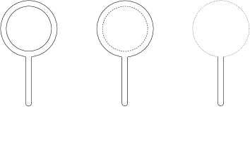
Figure 2: Tadpole diagrams contributing to the one-instanton contribution to $a_{i}$.

The first two diagrams contribute to $\langle{{\rm tr}\,\Psi_{ii}}\rangle\big{|}_{\rm sphere}$. These were evaluated in [5] with the result

$$\langle{{\rm tr}\,\Psi_{ii}}\rangle\big{|}_{\rm sphere}={1\over\alpha g_{s}}\sum_{j\neq i}\left[-\frac{S_{i}^{2}}{R_{i}e_{ij}}+2\frac{S_{i}S_{j}}{R_{i}e_{ij}}\right]\,.$$ (4.8)

The third diagram in figure 2 contributes to $\langle{{\rm tr}\,\Psi_{ii}}\rangle\big{|}_{\rm disk}$. By using the Feynman rules derived from the action (2.13) one finds

$$\langle{{\rm tr}\,\Psi_{ii}}\rangle\big{|}_{\rm disk}=-\,{S_{i}\over\alpha R_{i}}\sum_{I=1}^{N_{f}}\frac{1}{f_{iI}}\,.$$ (4.9)

Inserting the above results into eq. (4.7), evaluating the resulting expression using eq. (3.10), and using the identity (3.11), one finds

$$a_{i}=e_{i}+\Lambda^{2N-N_{f}}\left(-{2L_{i}\over R_{i}^{2}}\sum_{j\neq i}\frac{1}{e_{ij}}+{L_{i}\over R_{i}^{2}}\sum_{I=1}^{N_{f}}\frac{1}{f_{iI}}-{2\tilde{T}(e_{i})\over R_{i}}\right)+\mathcal{O}(\Lambda^{4N-2N_{f}})\,.$$ (4.10)

The relation between $a_{i}$ and $e_{i}$ that we have just derived agrees precisely, at the one-instanton level, with eq. (3.10) of ref. [25], provided that the polynomial $T(x)$ in their expression is set equal to ${\textstyle\frac{1}{2}}\tilde{T}(x)$. We will discuss the implications of this result in section 6.

5 Perturbative calculation of $\tau_{ij}(a)$ and $\mathcal{F}(a)$

Now that we have determined the relation between $a_{i}$ and $e_{i}$, we can rewrite $\tau_{ij}(e)$ in terms of $a_{i}$, and from that determine the form of the prepotential $\mathcal{F}(a)$ to one-instanton accuracy. Equation (4.10) implies that

$$\log e_{ij} = \log a_{ij}+\Lambda^{2N-N_{f}}\bigg{[}\sum_{k\neq i,j}\left({2L_{i}\over R_{i}^{2}e_{ij}e_{ik}}+{2L_{j}\over R_{j}^{2}e_{ji}e_{jk}}\right)+{2L_{i}\over R_{i}^{2}e_{ij}^{2}}+{2L_{j}\over R_{j}^{2}e_{ij}^{2}}$$ (5.1)

$$-\sum_{I=1}^{N_{f}}\left({L_{i}\over R_{i}^{2}e_{ij}f_{iI}}+{L_{j}\over R_{j}^{2}e_{ji}f_{jI}}\right)+{2\tilde{T}(e_{i})\over R_{i}e_{ij}}+{2\tilde{T}(e_{j})\over R_{j}e_{ji}}\bigg{]}\,,$$

where $a_{ij}=a_{i}-a_{j}$, and

$$\log f_{iI}=\log(a_{i}+m_{I})+\Lambda^{2N-N_{f}}\left[\sum_{k\neq i}{2L_{i}\over R_{i}^{2}e_{ik}f_{iI}}-{L_{i}\over R_{i}^{2}f_{iI}}\sum_{J=1}^{N_{f}}\frac{1}{f_{iJ}}+{2\tilde{T}(e_{i})\over R_{i}f_{iI}}\right]\,.$$ (5.2)

We can now re-express $\tau_{ij}$ (3.15) in terms of $a_{i}$

$$\tau_{ij}(a)=\tau_{ij}^{\rm pert}(a)+\sum_{d=1}^{\infty}\Lambda^{(2N-N_{f})d}\tau_{ij}^{(d)}(a)\,,$$ (5.3)

where the perturbative contribution is (up to additive constants)

$$2\pi i\tau^{\rm pert}_{ij}(a)=\delta_{ij}\Bigg{[}-\sum_{k\neq i}\log\left(a_{i}-a_{k}\over\Lambda\right)^{2}+\sum_{I=1}^{N_{f}}\log\left(a_{i}+m_{I}\over\Lambda\right)\Bigg{]}+(1-\delta_{ij})\Bigg{[}\log\left(a_{i}-a_{j}\over\Lambda\right)^{2}\Bigg{]}$$ (5.4)

and the one-instanton contribution is

$$2\pi i\tau^{(1)}_{ij}(a) = \delta_{ij}\Bigg{[}\sum_{k\neq i}\left({4L_{i}\over R_{i}^{2}}\sum_{\ell\neq i,k}{1\over a_{ik}a_{i\ell}}+{6L_{i}\over R_{i}^{2}a_{ik}^{2}}+{6L_{k}\over R_{k}^{2}a_{ik}^{2}}\right)$$

$$\;\;\;+\sum_{I=1}^{N_{f}}\left(-\sum_{k\neq i}{4L_{i}\over R_{i}^{2}a_{ik}f_{iI}}+\sum_{J\neq I}{L_{i}\over R_{i}^{2}f_{iI}f_{iJ}}\right)\Bigg{]}$$

$$+(1-\delta_{ij})\Bigg{[}\sum_{k\neq i,j}\left(-{4L_{i}\over R_{i}^{2}a_{ij}a_{ik}}-{4L_{j}\over R_{j}^{2}a_{ji}a_{jk}}+{4L_{k}\over R_{k}^{2}a_{ik}a_{jk}}\right)-{6L_{i}\over R_{i}^{2}a_{ij}^{2}}-{6L_{j}\over R_{j}^{2}a_{ij}^{2}}$$

$$\qquad\qquad\;+\sum_{I=1}^{N_{f}}\left({2L_{i}\over R_{i}^{2}e_{ij}f_{iI}}+{2L_{j}\over R_{j}^{2}e_{ji}f_{jI}}\right)\Bigg{]}\,,$$

where now $R_{i}=\prod_{j\neq i}(a_{i}-a_{j})$ and $f_{iI}=a_{i}+m_{I}$. Observe that all the $\tilde{T}(x)$ terms cancel out in the final expression for $\tau_{ij}(a)$. As will be discussed in more detail in the next section, $\tilde{T}(x)$ can be absorbed into a redefinition of the $e_{i}$ [25]. Since $\tau_{ij}(a)$ is independent of $e_{i}$ it should be insensitive to this redefinition, and therefore to the form of $\tilde{T}(x)$.

Finally, it is readily verified that (5.4), (5) can be written as $\tau_{ij}={\partial^{2}\mathcal{F}(a)/\partial a_{i}\partial a_{j}}$ with (up to a quadratic polynomial)

$$2\pi i\mathcal{F}(a) = -{\textstyle\frac{1}{4}}\sum_{i}\sum_{j\neq i}(a_{i}-a_{j})^{2}\log\left(a_{i}-a_{j}\over\Lambda\right)^{2}+{\textstyle\frac{1}{4}}\sum_{i}\sum_{I=1}^{N_{f}}(a_{i}+m_{I})^{2}\log\left(a_{i}+m_{I}\over\Lambda\right)^{2}$$ (5.6)

$$+\Lambda^{2N-N_{f}}\sum_{i}\prod_{j\neq i}\prod_{I=1}^{N_{f}}{(a_{i}+m_{I})\over(a_{i}-a_{j})^{2}}+\mathcal{O}(\Lambda^{4N-2N_{f}})\,.$$

This precisely agrees with the result obtained in eq. (4.34) of ref. [25].

To conclude, we have shown that a completely perturbative matrix model calculation, which does not use the Seiberg-Witten curve or differential, gives the correct result for the prepotential to first order in the instanton expansion for the $\mathrm{U}(N)$ gauge theory with $N_{f}$ fundamentals. Higher-instanton corrections to the prepotential may be obtained by higher-loop contributions to the matrix model free energy and tadpole diagrams.

6 The meaning of $\tilde{T}(x)$

In ref. [25] D’Hoker, Krichever, and Phong derived the prepotential for the $\mathcal{N}=2$ $\mathrm{U}(N)$ theory with $N_{f}$ flavors from a Seiberg-Witten curve of the form

$$y^{2}=\left[\prod_{i=1}^{N}(x-e_{i})+4\Lambda^{2N-N_{f}}T(x)\right]^{2}-4\Lambda^{2N-N_{f}}\prod_{I=1}^{N_{f}}(x+m_{I})\,.$$ (6.1)

In their work the $(N_{f}-N)$th order polynomial $T(x)$ was left unspecified (although two different candidates [8], [10] were presented) since, as shown in sec. II.c of that paper, the prepotential $\mathcal{F}(a)$ is independent of $T(x)$. This is because $T(x)$ can always be absorbed into a redefinition of the $e_{i}$, and $\mathcal{F}(a)$ is insensitive to a redefinition of $e_{i}$. However, since $T(x)$ is tied to the definition of $e_{i}$, its form will affect the relation between $a_{i}$ and $e_{i}$.

Our matrix model calculation of the relation between $a_{i}$ and $e_{i}$ (4.10) implies (via eq. (3.10) of ref. [25]) a specific form for $T(x)$, namely

$$T(x)={\textstyle\frac{1}{2}}\tilde{T}(x)+\mathcal{O}(\Lambda^{2N-N_{f}})={\textstyle\frac{1}{2}}\!\sum_{k=0}^{N_{f}-N}\tilde{t}_{k}x^{N_{f}-N-k}+\mathcal{O}(\Lambda^{2N-N_{f}})\,,$$ (6.2)

and thus corresponds to a specific choice of the $e_{i}$. (Our perturbative matrix model calculation only yields a result valid to one-instanton accuracy.) The Seiberg-Witten curve (6.1) corresponding to eq. (6.2) has the form

$$y^{2} = \prod_{i=1}^{N}(x-e_{i})^{2}-f(x)\,,$$

$$f(x) = 4\Lambda^{2N-N_{f}}\left(\prod_{I=1}^{N_{f}}(x+m_{I})-\tilde{T}(x)\prod_{i=1}^{N}(x-e_{i})\right)+\mathcal{O}(\Lambda^{4N-2N_{f}})\,.$$ (6.3)

The definition of $\tilde{T}(x)$, given below eq. (3.12), ensures that $f(x)$ is at most an $(N-1)$th order polynomial. Thus, the choice of $e_{i}$ in the matrix model is such that none of the coefficients of $x^{N}$ or higher powers in $y^{2}$ receive $O(\Lambda^{2N-N_{f}})$ corrections. (However, as we discuss below, the gauge-invariants $\langle{u_{n}}\rangle$ do receive corrections.) As we will see in the next section, this is exactly what the saddle-point solution of the matrix model requires.

It is curious to note that the form of $T(x)$ proposed in ref. [10] and on the right hand side of eq. (2.8) in ref. [25] is $T(x)={1\over 4}\sum_{k=0}^{N_{f}-N}\tilde{t}_{k}x^{N_{f}-N-k}$, precisely one-half of that in eq. (6.2). Why the difference?

Consider the gauge-invariant variables $\langle{u_{n}}\rangle={1\over n}\langle{{\rm tr}(\phi^{n})}\rangle$, which classically have the values $(u_{n})_{\rm cl}=(1/n)\sum_{i=1}^{N}e_{i}^{n}$. Quantum mechanically, these may be computed via [4, 5] $\langle{u_{n}}\rangle=(1/2\pi in)\sum_{i=1}^{N}\oint_{A_{i}}x^{n-1}\lambda_{SW}$, where $\lambda_{SW}$ is the Seiberg-Witten differential. They may also be computed in the matrix model [5], starting from the correlators $\langle{{\rm tr}(\Phi^{n})}\rangle$ (and modifying the expressions of ref. [5] to include the $\langle{{\rm tr}(\Phi^{n})}\rangle|_{\rm disk}$ contribution, as in eq. (4.7) of this paper; see sec. 8). It is easily shown that for $N_{f}<N$ (in which case $T(x)$ vanishes) $\langle{u_{n}}\rangle=(u_{n})_{\rm cl}$ for $n=1,\cdots,N$ [21, 5]. When $N_{f}\geq N$, however, $\langle{u_{n}}\rangle$ with $2N-N_{f}\leq n\leq N$ can get $\mathcal{O}(\Lambda^{2N-N_{f}})$ corrections.

As stated above, choosing a particular $T(x)$ corresponds to a particular choice of parameters $e_{i}$ used to parametrize the moduli space. It is possible to define the $N$ parameters $e_{i}$ so that the relation $\langle{u_{n}}\rangle=(1/n)\sum_{i=1}^{N}e_{i}^{n}$ continues to hold quantum mechanically for $n=1,\cdots,N$. This requirement then leads to the form of $T(x)$ in ref. [10] [25] (see however ref. [26]). In contrast, for the choice of $T(x)$ in eq. (6.2), $\langle{u_{n}}\rangle=(u_{n})_{\rm cl}$ no longer holds at the one-instanton level.

7 Matrix model derivation of the Seiberg-Witten curve

In this section, we will derive the form of the Seiberg-Witten curve for $\mathcal{N}=2$ U($N$) gauge theory with $N_{f}<2N$ fundamental hypermultiplets by solving the matrix model integral using saddle-point methods (for a review of this method, see, e.g., ref. [27]).

Our starting point is the matrix model partition function (2.4)

$$Z={1\over\mathrm{vol}(G)}\int{\rm d}\Phi\,{\rm d}Q^{I}{\rm d}\tilde{Q}_{I}\exp\left(-\frac{1}{g_{s}}W_{0}(\Phi)-{1\over g_{s}}\sum_{I=1}^{N_{f}}\left[\tilde{Q}_{I}\phi\,Q^{I}+m_{I}\tilde{Q}_{I}Q^{I}\right]\right)\,.$$ (7.1)

Diagonalizing $\Phi$ and integrating over $Q$, $\tilde{Q}$, one obtains ($\lambda_{i}$ are the eigenvalues of $\Phi$) [1, 16]

$$Z\propto\int\prod_{i=1}^{M}{\rm d}\lambda_{i}\exp\left(-\frac{1}{g_{s}}\sum_{i}W_{0}(\lambda_{i})+2\sum_{i<j}\log(\lambda_{i}-\lambda_{j})-\sum_{I=1}^{N_{f}}\sum_{i}\log(\lambda_{i}+m_{I})\right)$$ (7.2)

The saddle-point equation is obtained by varying the action with respect to $\lambda_{i}$:

$$-{1\over g_{s}}W^{\prime}_{0}(\lambda_{i})+2\sum_{j\not=i}{1\over\lambda_{i}-\lambda_{j}}-\sum_{I=1}^{N_{f}}{1\over\lambda_{i}+m_{I}}=0\,.$$ (7.3)

To solve (7.3), it is standard procedure [27] to introduce the trace of the resolvent

$$\omega(x)=\frac{1}{M}{\rm tr}\left(\frac{1}{\Phi-x}\right)={1\over M}\sum_{i}{1\over\lambda_{i}-x}$$ (7.4)

which can be shown to satisfy [27]

$$\omega^{2}(x)+{W^{\prime}_{0}(x)\over g_{s}M}\,\omega(x)+{1\over g_{s}M^{2}}\sum_{i}{W^{\prime}_{0}(x)-W^{\prime}_{0}(\lambda_{i})\over x-\lambda_{i}}$$ (7.5)

$$-{1\over M}\omega^{\prime}(x)+{1\over M^{2}}\sum_{i}\sum_{I=1}^{N_{f}}{1\over(\lambda_{i}-x)(\lambda_{i}+m_{I})}=0\,.$$

Now we let $g_{s}\rightarrow 0$, $M\to\infty$, with $S=g_{s}M$ held fixed. We also hold $N_{f}$ fixed; in this, our approach differs from ref. [16]. In this limit, the last two terms of eq. (7.5) vanish.

The large-$M$ limit expressions are conveniently written in terms of the density of eigenvalues

$$\rho(\lambda)={1\over M}\sum_{i}\delta(\lambda-\lambda_{i})\,,\qquad\qquad\int\rho(\lambda)\,{\rm d}\lambda=1\,.$$ (7.6)

In this language the resolvent becomes

$$\omega(x)=\int{\rm d}\lambda{\rho(\lambda)\over\lambda-x}\,,\qquad\qquad\rho(\lambda)={1\over 2\pi i}\left[\omega(\lambda+i\epsilon)-\omega(\lambda-i\epsilon)\right]$$ (7.7)

and eq. (7.5) can be rewritten as

$$\omega^{2}(x)+{W^{\prime}_{0}(x)\over S}\omega(x)+{1\over 4S^{2}}f(x)=0$$ (7.8)

where

$$f(x)=4S\int{\rm d}\lambda\,\rho(\lambda)\,{W_{0}^{\prime}(x)-W_{0}^{\prime}(\lambda)\over x-\lambda}$$ (7.9)

is an (as yet) arbitrary $(N-1)$th order polynomial. Defining

$$y(x)=2S\omega(x)+W^{\prime}_{0}(x)$$ (7.10)

one may rewrite eq. (7.8) as

$$y^{2}=W^{\prime}_{0}(x)^{2}-f(x),\qquad f(x)=\sum_{n=0}^{N-1}b_{n}x^{n}\,.$$ (7.11)

This equation characterizes a hyperelliptic Riemann surface. When the roots of $W^{\prime}_{0}(x)$ are well-separated and $f(x)$ is a small correction to $W^{\prime}_{0}(x)$, the curve has $N$ cuts in the $x$ plane, centered approximately on the roots of $W^{\prime}_{0}(x)$. The eigenvalues of $\Phi$ are clustered along these cuts. The function $f(x)$ determines the distribution of the eigenvalues of $\Phi$ among the $N$ cuts, and the spreading of those eigenvalues due to eigenvalue repulsion. Let $M_{i}$ denote the number of eigenvalues along the ${i^{\rm th}~{}{\rm cut}}$:

$$M_{i}=M\int_{i}{\rm d}\lambda\,\rho(\lambda)\,.$$ (7.12)

Define $S_{i}=g_{s}M_{i}$, which remains finite in the $M$, $M_{i}\to\infty$ limit. Then, using eqs. (7.7) and (7.10), we see that eq. (7.12) may be rewritten

$$S_{i}=\,-\,{1\over 4\pi i}\oint_{A_{i}}y\,{\rm d}x$$ (7.13)

where $A_{i}$ denotes the contour surrounding the $i$th cut. This is eq. (3.10) of [1] (up to a factor of 2; the sign depends on the direction of the contour integrals, which we take to be counterclockwise). Up to this point, we have just been following ref. [1].

As in ref. [21], we denote by $P$ and $Q$ the points $x=\infty$ on the two sheets of the curve (7.11). (If one needs a cutoff for an integral, one takes $P$ and $Q$ to be at $x=\Lambda_{0}$ with $\Lambda_{0}$ large.) To be specific, let $P$ be on the sheet on which $W^{\prime}_{0}(x)-y(x)$ goes to zero as $x\to\infty$. Also, denote by $C_{i}$ a path from $Q$ to $P$ that passes through the ${i^{\rm th}~{}{\rm cut}}$. The Riemann surface of genus $N-1$ described by the curve (7.11) can be given a canonical homology basis as follows: $A_{i}$ ($i=1,\ldots,N-1$) and $B_{i}=C_{i}-C_{N}$ ($i=1,\ldots,N-1$).

Our goal in the remainder of this section is to use matrix-model methods to determine the explicit form of $f(x)$ in the spectral curve (7.11). This will in turn yield the (hyperelliptic) Seiberg-Witten curve for the U($N$) theory with $N_{f}$ fundamental hypermultiplets. The saddle-point evaluation of the partition function (7.2) gives (here we need to keep the first subleading term since it contributes to $F_{\rm d}$)

$$Z = \exp\Bigg{(}-{S\over g_{s}^{2}}\int{\rm d}\lambda\,\rho(\lambda)\,W_{0}(\lambda)+{S^{2}\over g_{s}^{2}}\int{\rm d}\lambda\,{\rm d}\lambda^{\prime}\,\rho(\lambda)\,\rho(\lambda^{\prime})\log(\lambda-\lambda^{\prime})$$ (7.14)

$$\qquad\;\;-{S\over g_{s}}\sum_{I=1}^{N_{f}}\int{\rm d}\lambda\,\rho(\lambda)\,\log(\lambda+m_{I})\Bigg{)}$$

from which we infer

$$F_{\rm s}=-S\int{\rm d}\lambda\,\rho(\lambda)\,W_{0}(\lambda)+S^{2}\int{\rm d}\lambda\,{\rm d}\lambda^{\prime}\,\rho(\lambda)\,\rho(\lambda^{\prime})\,\log(\lambda-\lambda^{\prime})$$ (7.15)

and

$$F_{\rm d}=-S\sum_{I=1}^{N_{f}}\int{\rm d}\lambda\,\rho(\lambda)\,\log(\lambda+m_{I})\,.$$ (7.16)

In order to compute $W_{\rm eff}$, we need the variation of $F_{\rm s}$ under a small change in $S_{i}$. From (7.12) we see that such a variation can be implemented by letting $\rho(\lambda)\to\rho(\lambda)+(\delta S_{i}/S)\delta(\lambda-e_{i})$ where $e_{i}$ refers to an arbitrary, but fixed, point along the ${i^{\rm th}~{}{\rm cut}}$. Using this result in (7.15) gives

$$\delta F_{\rm s}=\delta S_{i}\left[-W_{0}(e_{i})+2S\int{\rm d}\lambda\,\rho(\lambda)\,\log(\lambda-e_{i})\right]\,.$$ (7.17)

This may be rewritten as (here const refers to a constant of integration)

$${\partial F_{\rm s}\over\partial S_{i}} = \int_{e_{i}}^{P}{\rm d}x~{}W^{\prime}_{0}(x)-2S\int{\rm d}\lambda\,\rho(\lambda)\int_{e_{i}}^{P}{{\rm d}x\over x-\lambda}+{\rm const}$$ (7.18)

$$= \int_{e_{i}}^{P}{\rm d}x\left(W^{\prime}_{0}(x)+2S\,\omega(x)\right)+{\rm const}$$

$$= \int_{e_{i}}^{P}y\,{\rm d}x+{\rm const}$$

which is just eq. (3.11) of [1]. Using the fact that $y$ differs only by a sign on the two sheets, together with the definition $B_{i}=C_{i}-C_{N}$, we may rewrite this as

$${\partial F_{\rm s}\over\partial S_{i}} = {\textstyle\frac{1}{2}}\int_{Q}^{e_{i}}y\,{\rm d}x+{\textstyle\frac{1}{2}}\int_{e_{i}}^{P}y\,{\rm d}x+{\rm const}$$ (7.19)

$$= {\textstyle\frac{1}{2}}\int_{C_{i}}y\,{\rm d}x+{\rm const}$$

$$= {\textstyle\frac{1}{2}}\int_{B_{i}}y\,{\rm d}x+{\textstyle\frac{1}{2}}\int_{C_{N}}y\,{\rm d}x+{\rm const}\,.$$

For $W_{\rm eff}$, we will also need

$$F_{\rm d}(e,S) = -S\sum_{I=1}^{N_{f}}\int{\rm d}\lambda\,\rho(\lambda)\int_{-m_{I}}^{P}{{\rm d}x\over\lambda-x}+{\rm const}$$ (7.20)

$$= -S\sum_{I=1}^{N_{f}}\int_{-m_{I}}^{P}\omega(x)\,{\rm d}x+{\rm const}$$

$$= -{\textstyle\frac{1}{2}}\sum_{I=1}^{N_{f}}\int_{-m_{I}}^{P}y(x)\,{\rm d}x+{\rm const}$$

where we absorb the $S_{i}$-independent $W_{0}(P)-W_{0}(-m_{I})$ terms into the integration constant.

We now use eqs. (7.19) and (7.20) in the effective superpotential (setting $N_{i}=1$)

$$\!W_{\rm eff}\! = \!\!-\sum_{i=1}^{N}{\partial F_{\rm s}\over\partial S_{i}}-F_{\rm d}+2\pi i\tau_{0}\sum_{i=1}^{N}S_{i}$$ (7.21)

$$= \!\!-{\textstyle\frac{1}{2}}\sum_{i=1}^{N-1}\oint_{B_{i}}\!y\,{\rm d}x-{\textstyle\frac{1}{2}}N\int_{C_{N}}\!\!y\,{\rm d}x+{\textstyle\frac{1}{2}}\sum_{I=1}^{N_{f}}\int_{-m_{I}}^{P}\!\!y\,{\rm d}x-{\textstyle\frac{1}{2}}\tau_{0}\sum_{i=1}^{N}\oint_{A_{i}}\!\!y\,{\rm d}x+{\rm const}.$$

In the prescription relating the matrix model and the $\mathcal{N}=2$ gauge theory we are instructed to extremize $W_{\rm eff}$ with respect to $S_{i}$. Since the $S_{i}$’s are determined by $f(x)$ and therefore by the $b_{n}$’s through eqs. (7.11) and (7.13), we may equivalently vary (7.21) with respect to $b_{n}$ [21]. From eq. (7.11), one sees that $(\partial y/\partial b_{n}){\rm d}x=-{\textstyle\frac{1}{2}}x^{n}{\rm d}x/y$. For $0\leq n\leq N-2$, these form a complete basis of holomorphic differentials on the Riemann surface [29]. We may therefore change basis to the unique basis of holomorphic differentials $\zeta_{k}$ dual to the homology basis, i.e., $\oint_{A_{i}}\zeta_{k}=\delta_{ik}$. Consequently, the equations $\delta W_{\rm eff}/\delta b_{n}=0$ for $0\leq n\leq N-2$ may be rewritten

$$0=-\sum_{i=1}^{N-1}\oint_{B_{i}}\zeta_{k}-N\int_{Q}^{P}\zeta_{k}+\sum_{I=1}^{N_{f}}\int_{-m_{I}}^{P}\zeta_{k}$$ (7.22)

where $\sum_{i=1}^{N}\oint_{A_{i}}\zeta_{k}=0$ because the sum of $A_{i}$ cycles is a trivial cycle. The first term just yields $\sum_{i=1}^{N-1}\tau_{ik}$, which is an element of the period lattice. Hence

$$N\int_{P}^{Q}\zeta_{k}+\sum_{I=1}^{N_{f}}\int_{-m_{I}}^{P}\zeta_{k}=$$

$$N\int_{p_{0}}^{Q}\zeta_{k}-(N-N_{f})\int_{p_{0}}^{P}\zeta_{k}-\sum_{I=1}^{N_{f}}\int_{p_{0}}^{-m_{I}}\zeta_{k}=0\quad{\rm(modulo~{}the~{}period~{}lattice)}$$ (7.23)

where $p_{0}$ is an arbitrary (generic) point on the Riemann surface. It now follows from Abel’s theorem [29] that there exists a function $\psi(x)$ on the Riemann surface with an $N$th order pole at $Q$, an $(N-N_{f})$th order zero (or pole, if $N_{f}>N$) at $P$, and simple zeros at $-m_{I}$ for $I=1,\ldots,N_{f}$. As we will now show, this requirement suffices to fix the form of $f(x)$, and therefore the Seiberg-Witten curve.

For $0\leq N_{f}<N$, the function $\psi(x)$ is simply (proportional to) the resolvent:

$$\psi(x)=y-W^{\prime}_{0}(x)=\sqrt{W^{\prime}_{0}(x)^{2}-f(x)}-W^{\prime}_{0}(x),\qquad 0\leq N_{f}<N$$ (7.24)

This can be seen as follows: $\psi(x)$ has an $N$th order pole at $Q$, and (at least) a simple zero at $P$ (because $f(x)$ is a polynomial of at most $(N-1)$th order). Abel’s theorem yields $N-1$ conditions and therefore completely constrains the remaining zeros. Thus $\psi(x)$ must have a simple zero at $x=-m_{I}$, so $f(x)$ must contain a factor $(x+m_{I})$ for each $I$. For $\psi(x)$ to have an $(N-N_{f})$th order zero at $P$, $f(x)$ can be of $N_{f}$th order at most. These two conditions require $f(x)\propto\prod_{I=1}^{N_{f}}(x+m_{I})$. Naming the constant of proportionality $4\Lambda^{2N-N_{f}}$, and setting $\alpha=1$ in eq. (2.2), we see that the spectral curve (7.11) is given by

$$y^{2}=\prod_{i=1}^{N}(x-e_{i})^{2}-4\Lambda^{2N-N_{f}}\prod_{I=1}^{N_{f}}(x+m_{I})$$ (7.25)

precisely the Seiberg-Witten curve [7]–[10] for $N_{f}<N$. (It should also be possible to determine this constant of proportionality by setting $\delta W_{\rm eff}/\delta b_{N-1}=0$, and using the gauge theory relation $2\pi i\tau(\Lambda_{0})=(2N-N_{f})\log(\Lambda/\Lambda_{0})$ and the fact that [21] $\sum_{i=1}^{N}\oint_{A_{i}}\!\!y\,{\rm d}x=-\pi ib_{N-1}$.)

For $N\leq N_{f}<2N$, the function $\psi(x)$ is not given by the resolvent but by a related function

$$\psi(x)=\sqrt{A(x)^{2}-g(x)}-A(x),\qquad N\leq N_{f}<2N$$ (7.26)

where $A(x)$ is an $N$th order polynomial and $g(x)\propto\prod_{I=1}^{N_{f}}(x+m_{I})$. (As before, we name the proportionality constant $4\Lambda^{2N-N_{f}}$.) Under these conditions, $\psi(x)$ vanishes at $x=-m_{I}$, for $I=1,\ldots N_{f}$, has an $N$th order pole at $Q$, and an $(N_{f}-N)$th order pole at $P$. For $\psi(x)$ to be a function on the Riemann surface (7.11), the square root in $\psi(x)$ must be proportional to $y(x)$, that is (normalizing appropriately)

$$A(x)^{2}-4\Lambda^{2N-N_{f}}\prod_{I=1}^{N_{f}}(x+m_{I})=W^{\prime}_{0}(x)^{2}-f(x)$$ (7.27)

where $f(x)$ is a polynomial of order at most $(N-1)$. The solution to this, to $\mathcal{O}(\Lambda^{2N-N_{f}})$, is

$$A(x) = \prod_{i=1}^{N}(x-e_{i})+2\Lambda^{2N-N_{f}}\tilde{T}(x),$$

$$f(x) = 4\Lambda^{2N-N_{f}}\left(\prod_{I=1}^{N_{f}}(x+m_{I})-\tilde{T}(x)\prod_{i=1}^{N}(x-e_{i})\right)$$ (7.28)

where $\tilde{T}(x)$ is defined below eq. (3.12), and again we have set $\alpha=1$ in eq. (2.2). Thus the spectral curve (7.11) and function $\psi(x)$ are given by

$$y^{2} = \prod_{i=1}^{N}(x-e_{i})^{2}-f(x),\qquad N\leq N_{f}<2N$$

$$\psi(x) = y-A(x),$$ (7.29)

in agreement with the Seiberg-Witten curve for $N\leq N_{f}<2N$ [7]–[10] but with a particular choice of subleading term $\tilde{T}(x)$. (This form of the curve was already obtained (6) in the previous section by comparing our perturbative matrix model calculation with the curve in ref. [25]. The subleading term $\tilde{T}(x)$ simply corresponds to a particular choice of moduli parameters $e_{i}$ picked out by the matrix model.)

Thus, for both $N_{f}<N$ and $N\leq N_{f}<2N$, the spectral curve obtained from the matrix-model saddle-point integral agrees precisely with the known Seiberg-Witten curve (6.1) for the $\mathcal{N}=2$ U($N$) gauge theory with $N_{f}$ fundamental hypermultiplets.

Finally, from the properties of $\psi(x)$ (7.24), (7.26), we see that

$$h(x){\rm d}x={{\rm d}\psi\over\psi}$$ (7.30)

is a meromorphic differential with simple poles at $P$, $Q$, and $x=-m_{I}$ and residues $N-N_{f}$, $-N$, and $1$ respectively. These conditions imply that the meromorphic differential given by $\lambda_{SW}=x\,h(x){\rm d}x$ has all the correct properties to be the Seiberg-Witten differential [7, 10, 30]. Moreover, using the specific forms of $\psi(x)$ given in eqs. (7.25) and (7), we obtain exactly the form of the $\lambda_{SW}$ given in ref. [25].

8 Derivation of the Seiberg-Witten differential

In the previous section we obtained an expression (7.30) related to the Seiberg-Witten differential $\lambda_{SW}$. Although this form can be motivated from the Calabi-Yau approach [21, 31] it does not constitute a genuine matrix-model derivation of $\lambda_{SW}$. In this section we present a derivation of $\lambda_{SW}$ entirely within the framework of the matrix model.

In the Seiberg-Witten approach, the gauge-theory expectation value of ${\rm tr}\,\phi^{n}$ is calculated via [4, 5]

$$\langle{{\rm tr}\,\phi^{n}}\rangle=\frac{1}{2\pi i}\sum_{i=1}^{N}\oint_{A_{i}}x^{n-1}\lambda_{SW}\,.$$ (8.1)

The relation between the gauge theory vev and matrix model quantities is

$$\langle{{\rm tr}\,\phi^{n}}\rangle=\left[\sum_{j=1}^{N}{\partial\over\partial S_{j}}g_{s}\langle{{\rm tr}\Phi^{n}}\rangle_{\mathrm{sphere}}+\langle{{\rm tr}\,\Phi^{n}}\rangle_{\mathrm{disk}}\right]\bigg{|}_{\langle{S}\rangle}$$ (8.2)

which generalizes eq. (5.10) in ref. [5] to the case when boundaries are present (see also [15]). The derivation of eq. (8.2) is similar to that of eq. (4.7) of this paper but uses the deformation $\tilde{W}(\Phi,Q,\tilde{Q})=W(\Phi,Q,\tilde{Q})+\epsilon\,(1/n)\,{\rm tr}\,(\Phi^{n})$.

The matrix-model expectation values $\langle{{\rm tr}\,\Phi^{n}}\rangle$ in eq. (8.2) may be expressed in terms of the resolvent (7.4)

$$\omega(x) = \,-\,\frac{1}{M}\left\langle{\rm tr}\frac{1}{x-\Phi}\right\rangle=\,-\,\frac{1}{M}\sum_{n=0}^{\infty}x^{-n-1}\langle{{\rm tr}\,\Phi^{n}}\rangle$$

$$\langle{{\rm tr}\,\Phi^{n}}\rangle = -\,\frac{M}{2\pi i}\sum_{i=1}^{N}\oint_{A_{i}}x^{n}\,\omega(x)\,{\rm d}x$$ (8.3)

which acts as a generating function for the expectation values. To proceed, we rewrite the last term in (7.5) as

$${1\over M^{2}}\sum_{i}\sum_{I=1}^{N_{f}}{1\over(\lambda_{i}-x)(\lambda_{i}+m_{I})} = {1\over M^{2}}\sum_{i}{1\over\lambda_{i}-x}\sum_{I=1}^{N_{f}}{1\over x+m_{I}}\,-\,{1\over M^{2}}\sum_{I=1}^{N_{f}}{1\over x+m_{I}}\sum_{i}{1\over\lambda_{i}+m_{I}}$$ (8.4)

$$= {1\over M}\sum_{I=1}^{N_{f}}{\omega(x)-\omega(-m_{I})\over x+m_{I}}$$

so that eq. (7.5) becomes

$$\omega^{2}(x)+{W^{\prime}_{0}(x)\over g_{s}M}\,\omega(x)+{1\over g_{s}M^{2}}\sum_{i}{W^{\prime}_{0}(x)-W^{\prime}_{0}(\lambda_{i})\over x-\lambda_{i}}$$ (8.5)

$$-{1\over M}\omega^{\prime}(x)+{1\over M}\sum_{I=1}^{N_{f}}{\omega(x)-\omega(-m_{I})\over x+m_{I}}=0\,.$$

Next, we expand $\omega(x)$ as

$$\omega(x)=\sum_{\chi\leq 2}\frac{1}{M^{2-\chi}}\omega_{1-\chi/2}(x)=\omega_{0}(x)+\frac{1}{M}\omega_{1/2}(x)+\mathcal{O}(\frac{1}{M^{2}})\,.$$ (8.6)

Using the method developed in ref. [32], we can solve the loop-equation (8.5) order-by-order in $1/M$, which in principle will give us $\langle{{\rm tr}\,\Phi^{n}}\rangle$ to arbitrary order in the topological expansion. For eq. (8.2), however, we will only need $\omega_{\rm s}(x)\equiv\omega_{0}(x)$ and $\omega_{\rm d}(x)\equiv\omega_{1/2}(x)$. Inserting (8.6) into eq. (8.5), and using the fact [32] that the $(1/M)\omega^{\prime}(x)$ term is $\mathcal{O}(1/M^{2})$, we find

$$\omega_{\rm s}(x) = {1\over 2S}\left[y-W^{\prime}_{0}(x)\right]\,,$$

$$\omega_{\rm d}(x) = -\frac{S}{y}\sum_{I=1}^{N_{f}}\frac{\omega_{\rm s}(x)-\omega_{\rm s}(-m_{I})}{x+m_{I}}\,,$$ (8.7)

where $y^{2}=W_{0}^{\prime}(x)^{2}-f(x)$. This result, together with (8), allows us to write the contributions to $\langle{{\rm tr}\,\Phi^{n}}\rangle$ at the sphere ($\chi=2$) and disk ($\chi=1$) levels as

$$\langle{{\rm tr}\,\Phi^{n}}\rangle_{\mathrm{sphere}} = -\,\frac{M}{2\pi i}\sum_{i=1}^{N}\oint_{A_{i}}x^{n}\,\omega_{\rm s}(x)\,{\rm d}x\,,$$

$$\langle{{\rm tr}\,\Phi^{n}}\rangle_{\mathrm{disk}} = -\,\frac{1}{2\pi i}\sum_{i=1}^{N}\oint_{A_{i}}x^{n}\,\omega_{\rm d}(x)\,{\rm d}x\,.$$ (8.8)

Inserting these expressions into eq. (8.2) and comparing with (8.1) one can read off

$$\lambda_{SW}=x\left[\sum_{i=1}^{N}\frac{\partial}{\partial S_{i}}(-S\omega_{\rm s}(x))-\omega_{\rm d}(x)\right]\bigg{|}_{\langle{S}\rangle}{\rm d}x\,.$$ (8.9)

This generalizes eq. (5.3) in v3 of ref. [15] to the case when boundaries are present.

Using eq. (8), we have

$$\sum_{i=1}^{N}\frac{\partial}{\partial S_{i}}(-S\omega_{\rm s}(x))=\,-\,{\textstyle\frac{1}{2}}\sum_{i=1}^{N}\frac{\partial y}{\partial S_{i}}\,.$$ (8.10)

This expression has unit $A_{i}$-periods,

$$\frac{1}{2\pi i}\oint_{A_{i}}\left[-\,{\textstyle\frac{1}{2}}\sum_{j=1}^{N}\frac{\partial y}{\partial S_{j}}\right]\,{\rm d}x=\sum_{j=1}^{N}\frac{\partial}{\partial S_{j}}\left[-\,\frac{1}{4\pi i}\oint_{A_{i}}y\,{\rm d}x\right]=\sum_{j=1}^{N}\frac{\partial}{\partial S_{j}}S_{i}=1$$ (8.11)

using the definition of $S_{i}$ (7.13). Moreover, by writing ($b_{n}$ was defined in eq. (7.11) )

$$\,-\,{\textstyle\frac{1}{2}}\sum_{i=1}^{N}\frac{\partial y}{\partial S_{i}}=\,-\,{\textstyle\frac{1}{2}}\sum_{i=1}^{N}\sum_{n=0}^{N-1}\frac{\partial b_{n}}{\partial S_{i}}\frac{\partial y}{\partial b_{n}} = \,-\,{\textstyle\frac{1}{2}}\frac{\partial y}{\partial b_{N-1}}\sum_{i=1}^{N}\frac{\partial b_{N-1}}{\partial S_{i}}+{\rm holomorphic}$$ (8.12)

$$= {Nx^{N-1}\over y}+{\rm holomorphic}$$

we see that this expression has simple poles at $P$ and $Q$ with residues $\pm N$, and no other poles. The properties (8.11) and (8.12) suffice to show that

$$\,-\,{\textstyle\frac{1}{2}}\sum_{i=1}^{N}\frac{\partial y}{\partial S_{i}}=\frac{W_{0}^{\prime\prime}(x)}{y}$$ (8.13)

as the function on the r.h.s. has the same properties.

To simplify the remainder of the discussion, we consider $N_{f}<N$. In this case, we found in the previous section that $f(x)\propto\prod_{I=1}^{N_{f}}(x+m_{I})$, so $f(-m_{I})=0$. The contours in eq. (8) are on the sheet on which $y=+W^{\prime}_{0}(x)+\ldots$, and on this sheet, eqs. (7.10) and (7.11) imply $\omega_{\rm s}(-m_{I})=0$ so this term drops out of eq. (8), yielding

$$\omega_{\rm d}(x)=\,-\,\frac{y-W^{\prime}_{0}(x)}{2y}\sum_{I=1}^{N_{f}}\frac{1}{x+m_{I}}=\,-\,\frac{y-W^{\prime}_{0}(x)}{2y}{f^{\prime}\over f}$$ (8.14)

Collecting the above results one finds

$$\lambda_{SW}=\frac{x}{y}\left[W^{\prime\prime}_{0}(x)-{\textstyle\frac{1}{2}}(W^{\prime}_{0}(x)-y)\frac{f^{\prime}}{f}\right]$$ (8.15)

which is in perfect agreement with the $N_{f}<N$ result in ref. [25].

9 Summary

In this paper we have continued the program initiated in [5] for analyzing $\mathcal{N}=2$ gauge theories within the matrix model approach [1]–[4]; here we included matter in the fundamental representation of $\mathrm{U}(N)$. This addition exposes new features of the method, one of which is the appearance of disk diagrams that contribute to the free energy. Similarly, the tadpole diagrams necessary for computing the periods $a_{i}$ also have a contribution from disk diagrams. We computed the relation between $a_{i}$ and the classical moduli $e_{i}$, as well as the $\mathcal{N}=2$ prepotential $\mathcal{F}(a)$, finding complete agreement with known results.

An interesting feature of our calculation is that the two cases $N_{f}<N$ and $N\leq N_{f}<2N$ are on the same footing and can be treated using the same method within the matrix model approach. The only difference between the two cases is the appearance of the polynomial $\tilde{T}(x)$ when $N_{f}\geq N$, cf. (4.10). In the final expression for the prepotential, however, $\tilde{T}(x)$ disappears. In section 6 we discussed the meaning of $\tilde{T}(x)$, explaining how it affects the form of the Seiberg-Witten curve when $N_{f}\geq N$.

From the point of view of computational efficiency, the matrix model approach cannot, in its present form, compete with other methods for computing multi-instanton contributions [34]–[36]. However, it would be interesting to connect these approaches with the matrix model perspective to improve our understanding of multi-instanton effects.

In sections 7 and 8 we presented derivations, entirely within the context of the matrix model, of the Seiberg-Witten curve and differential for the $\mathcal{N}=2$ $\mathrm{U}(N)$ theory with $N_{f}<2N$ flavors. The contribution to the free energy from disk diagrams (7.20) played an important role in the analysis. A comparison of (7.24) and (7) exhibits the difference between the Seiberg-Witten curves for $N_{f}<N$ and $N\leq N_{f}<2N$. In the latter case, the matrix model makes a specific choice for the modification of the curve. This result was also inferred in sec. 6 from the perturbative calculation.

References

• [1] R. Dijkgraaf and C. Vafa, “Matrix models, topological strings, and supersymmetric gauge theories,” Nucl. Phys. B644 (2002) 3, hep-th/0206255.
• [2] R. Dijkgraaf and C. Vafa, “On geometry and matrix models,” Nucl. Phys.  B644 (2002) 21, hep-th/0207106.
• [3] R. Dijkgraaf and C. Vafa, “A perturbative window into non-perturbative physics,” hep-th/0208048.
• [4] R. Dijkgraaf, S. Gukov, V. A. Kazakov and C. Vafa, “Perturbative analysis of gauged matrix models,” hep-th/0210238.
• [5] S. Naculich, H. Schnitzer, and N. Wyllard, “The $\mathcal{N}=2$ $\mathrm{U}(N)$ gauge theory prepotential and periods from a perturbative matrix model calculation,” hep-th/0211123.
• [6] R. Argurio, V. L. Campos, G. Ferretti and R. Heise, “Exact superpotentials for theories with flavors via a matrix integral,” hep-th/0210291.
• [7] N. Seiberg and E. Witten, “Electric-magnetic duality, monopole condensation, and confinement in $\mathcal{N}=2$ supersymmetric Yang-Mills theory,” Nucl. Phys. B426 (1994) 19 [Erratum-ibid. B430 (1994) 485], hep-th/9407087; “Monopoles, duality and chiral symmetry breaking in $\mathcal{N}=2$ supersymmetric QCD,” Nucl. Phys. B431 (1994) 484, hep-th/9408099.
• [8] A. Hanany and Y. Oz, “On the quantum moduli space of vacua of $\mathcal{N}=2$ supersymmetric $\mathrm{SU}(N_{c})$ gauge theories,” Nucl. Phys. B452 (1995) 283, hep-th/9505075.
• [9] P. C. Argyres, M. R. Plesser and A. D. Shapere, “The Coulomb phase of $\mathcal{N}=2$ supersymmetric QCD,” Phys. Rev. Lett.  75 (1995) 1699, hep-th/9505100;
J. A. Minahan and D. Nemeschansky, “Hyperelliptic curves for supersymmetric Yang-Mills,” Nucl. Phys B464 (1996) 3, hep-th/9507032.
• [10] I. M. Krichever and D. H. Phong, “On the integrable geometry of soliton equations and $\mathcal{N}=2$ supersymmetric gauge theories,” J. Diff. Geom.  45 (1997) 349, hep-th/9604199.
• [11] A. Klemm, M. Mariño and S. Theisen, “Gravitational corrections in supersymmetric gauge theory and matrix models,” hep-th/0211216;
R. Dijkgraaf, A. Sinkovics and M. Temürhan, “Matrix models and gravitational corrections,” hep-th/0211241.
• [12] H. Itoyama and A. Morozov, “The Dijkgraaf-Vafa prepotential in the context of general Seiberg-Witten theory,” hep-th/0211245.
• [13] R. Dijkgraaf, M. T. Grisaru, C. S. Lam, C. Vafa and D. Zanon, “Perturbative computation of glueball superpotentials,” hep-th/0211017.
• [14] F. Cachazo, M. R. Douglas, N. Seiberg and E. Witten, “Chiral rings and anomalies in supersymmetric gauge theory,” hep-th/0211170.
• [15] R. Gopakumar, “$\mathcal{N}$ = 1 theories and a geometric master field,” hep-th/0211100.
• [16] J. McGreevy, “Adding flavor to Dijkgraaf-Vafa,” hep-th/0211009.
• [17] H. Suzuki, “Perturbative derivation of exact superpotential for meson fields from matrix theories with one flavour,” hep-th/0211052.
• [18] I. Bena and R. Roiban, “Exact superpotentials in $\mathcal{N}=1$ theories with flavor and their matrix model formulation,” hep-th/0211075.
• [19] Y. Demasure and R. A. Janik, “Effective matter superpotentials from Wishart random matrices,” hep-th/0211082.
• [20] B. Feng, “Seiberg duality in matrix model,” hep-th/0211202.
• [21] F. Cachazo and C. Vafa, “$\mathcal{N}=1$ and $\mathcal{N}=2$ geometry from fluxes,” hep-th/0206017.
• [22] G. ’t Hooft, “A planar diagram theory for strong interactions,” Nucl. Phys. B72 (1974) 461.
• [23] H. Ooguri and C. Vafa, “Worldsheet derivation of a large $N$ duality,” Nucl. Phys. B641 (2002) 3, hep-th/0205297.
• [24] F. Cachazo, K. Intriligator, and C. Vafa, “A large $N$ duality via a geometric transition,” Nucl. Phys. B603 (2001) 3, hep-th/0103067.
• [25] E. D’Hoker, I. M. Krichever and D. H. Phong, “The effective prepotential of $\mathcal{N}=2$ supersymmetric $\mathrm{SU}(N_{c})$ gauge theories,” Nucl. Phys. B489 (1997) 179, hep-th/9609041.
• [26] M. J. Slater, “One-instanton tests of the exact results in $\mathcal{N}=2$ supersymmetric QCD,” Phys. Lett. B 403 (1997) 57, hep-th/9701170.
• [27] P. Di Francesco, P. Ginsparg and J. Zinn-Justin, “2-D Gravity and random matrices,” Phys. Rept.  254 (1995) 1, hep-th/9306153.
• [28] F. Ferrari, “Quantum parameter space and double scaling limits in $\mathcal{N}=1$ super Yang-Mills theory,” hep-th/0211069.
• [29] H. M. Farkas and I. Kra, Riemann Surfaces, 2nd ed., Springer-Verlag, 1992.
• [30] I. M. Krichever and D. H. Phong, “Symplectic forms in the theory of solitons,” hep-th/9708170.
• [31] Y. Ookouchi, “$\mathcal{N}=1$ gauge theory with flavor from fluxes,” hep-th/0211287.
• [32] J. Ambjørn, L. Chekhov and Y. Makeenko, “Higher genus correlators from the hermitian one matrix model,” Phys. Lett. B282 (1992) 341, hep-th/9203009;
J. Ambjørn, L. Chekhov, C. Kristjansen and Y. Makeenko, “Matrix model calculations beyond the spherical limit,” Nucl. Phys. B404 (1993) 127 [Erratum-ibid. B449 (1995) 681], hep-th/9302014;
G. Akemann, “Higher genus correlators for the hermitian matrix model with multiple cuts,” Nucl. Phys. B482 (1996) 403, hep-th/9606004.
• [33] S. K. Ashok, R. Corrado, N. Halmagyi, K. D. Kennaway and C. Römelsberger, “Unoriented strings, loop equations, and $\mathcal{N}=1$ superpotentials from matrix models,” hep-th/0211291.
• [34] G. Chan and E. D’Hoker, “Instanton recursion relations for the effective prepotential in $\mathcal{N}=2$ super Yang-Mills,” Nucl. Phys. B564, 503 (2000) hep-th/9906193.
• [35] N. Dorey, T. J. Hollowood, V. V. Khoze and M. P. Mattis, “The calculus of many instantons,” hep-th/0206063.
• [36] N. A. Nekrasov, “Seiberg-Witten prepotential from instanton counting,” hep-th/0206161;
R. Flume and R. Poghossian, “An algorithm for the microscopic evaluation of the coefficients of the Seiberg-Witten prepotential,” hep-th/0208176;
U. Bruzzo, F. Fucito, J. F. Morales and A. Tanzini, “Multi-instanton calculus and equivariant cohomology,” hep-th/0211108.