SIMULATION OF INTERSECTING BLACK BRANE SOLUTIONS

BY MULTI-COMPONENT ANISOTROPIC FLUID

V.D. Ivashchuk,a,b,1 V.N. Melnikova,b,2 and A.B. Selivanova,3

a

Institute of Gravitation and Cosmology, Peoples Friendship University of Russia
6 Miklukho-Maklaya St., Moscow 117198, Russia

b

Centre for Gravitation and Fundamental Metrology, VNIIMS
3-1 M.Ulyanovoy St., Moscow 119313, Russia

A family of spherically symmetric solutions with horizon in the model with multi-component anisotropic fluid (MCAF) is obtained. The metric of any solution contains $(n-1)$ Ricci-flat β€œinternal space” metrics and for certain equations of state ($p_{i}=\pm\rho$) coincides with the metric of intersecting black brane solution in the model with antisymmetric forms. Examples of simulation of intersecting $M2$ and $M5$ black branes are considered. The post-Newtonian parameters $\beta$ and $\gamma$ corresponding to the 4-dimensional section of the metric are calculated.

PACS numbers:Β 04.20.Jb; 04.50.+h.

Keywords: $p$-brane, anisotropic fluid.

11footnotetext: e-mail: ivas@rgs.phys.msu.su22footnotetext: e-mail: melnikov@rgs.phys.msu.su33footnotetext: e-mail: seliv@rgs.phys.msu.su

1 Introduction

Recently, spherically-symmetric $p$-brane solutions with horizon (see, e.g., [1] and references therein) defined on product manifolds ${\bf R}\times M_{0}\times\ldots\times M_{n}$ cause a wide interest. These solutions appear in models with antisymmetric forms and scalar fields. These and more general $p$-brane cosmological and spherically symmetric solutions are usually obtained by reduction of the field equations to the Lagrange equations corresponding to Toda-like systems [4]. An analogous reduction for models with multi-component anisotropic fluids was performed earlier in [6]. For cosmological-type models with antisymmetric forms without scalar fields any $p$-brane is equivalent to an anisotropic fluid with the equations of state:

$$\hat{p}_{i}=-{\hat{\rho}}\qquad{\rm or}\qquad{\hat{p}}_{i}={\hat{\rho}},$$ (1.1)

when the manifold $M_{i}$ belongs or does not belong to the brane world volume, respectively (here ${\hat{p}}_{i}$ is the effective pressure in $M_{i}$ and ${\hat{\rho}}$ is the effective density).

In this paper we find the analogues of intersecting black brane solutions in a model with multi-component anisotropic fluid (MCAF), when certain ”orthogonality” relations on fluid parameters are imposed. The one-component case was considered earlier in [12].

The paper is organized as follows. In Section 2 the model is formulated. In Section 3 general MCAF solutions with horizon corresponding to black-brane-type solutions are presented. Section 4 deals with certain MCAF analogues of intersecting black brane solutions, i.e. $M2$ and $M5$ black brane solutions. In Section 5 the post-Newtonian parameters for the 4-dimensional section of the MCAF-black-brane metric are calculated. In Appendix based on [1, 7] the general spherically symmetric solutions with multicomponent anisotropic fluid are considered and configurations with horizon are singled out.

2 The model

In this paper we consider a family of spherically symmetric solutions to Einstein equations with an anisotropic matter source

$$R^{M}_{N}-\frac{1}{2}\delta^{M}_{N}R=kT^{M}_{N},$$ (2.1)

defined on the manifold

$$\begin{array}[]{l}M={{\bf R}}_{*}\times(M_{0}=S^{d_{0}})\times(M_{1}={{\bf R}})\times\ldots\times M_{n},\\ \qquad{}^{\rm radial\phantom{p}}_{\rm variable}\quad{}^{\rm spherical}_{\rm variables}\quad\qquad{}^{\rm time}\end{array}$$ (2.2)

with the block-diagonal metrics

$$ds^{2}={\,\rm e}^{2\gamma(u)}du^{2}+\sum^{n}_{i=0}{\,\rm e}^{2X^{i}(u)}h^{[i]}_{m_{i}n_{i}}dy^{m_{i}}dy^{n_{i}}.$$ (2.3)

Here ${\bf R}_{*}\subseteq{\bf R}$ is an open interval. The manifold $M_{i}$ with the metric $h^{[i]}$, $i=1,2,\ldots,n$, is a Ricci-flat space of dimension $d_{i}$:

$$R_{m_{i}n_{i}}[h^{[i]}]=0,$$ (2.4)

and $h^{[0]}$ is the standard metric on the unit sphere $S^{d_{0}}$, so that

$$R_{m_{0}n_{0}}[h^{[0]}]=(d_{0}-1)h^{[0]}_{m_{0}n_{0}};$$ (2.5)

$u$ is a radial variable, $\kappa$ is the gravitational constant, $d_{1}=1$ and $h^{[1]}=-dt\otimes dt$.

The energy-momentum tensor is adopted in the following form for each component of the fluid:

(T(s)NM)=diag​(βˆ’Ο^(s),p^0(s)​δk0m0,p^1(s)​δk1m1,…,p^n(s)​δknmn),subscriptsuperscriptsuperscript𝑇𝑠𝑀𝑁diagsuperscript^πœŒπ‘ superscriptsubscript^𝑝0𝑠subscriptsuperscript𝛿subscriptπ‘š0subscriptπ‘˜0superscriptsubscript^𝑝1𝑠subscriptsuperscript𝛿subscriptπ‘š1subscriptπ‘˜1…superscriptsubscript^𝑝𝑛𝑠subscriptsuperscript𝛿subscriptπ‘šπ‘›subscriptπ‘˜π‘›({T^{(s)}}^{M}_{N})={\rm diag}(-{\hat{\rho}^{(s)}},{\hat{p}}_{0}^{(s)}\delta^{m_{0}}_{k_{0}},{\hat{p}}_{1}^{(s)}\delta^{m_{1}}_{k_{1}},\ldots,{\hat{p}}_{n}^{(s)}\delta^{m_{n}}_{k_{n}}), (2.6)

where ρ^(s)superscript^πœŒπ‘ \hat{\rho}^{(s)} and $\hat{p}_{i}^{(s)}$ are the effective density and pressures respectively, depending on the radial variable $u$.

We assume that the following ”conservation laws”

$$\nabla_{M}T^{(s)M}_{\ N}=0$$ (2.7)

are valid for all components.

We also impose the following equations of state

p^i(s)=(1βˆ’2​Ui(s)di)​ρ^(s),superscriptsubscript^𝑝𝑖𝑠12superscriptsubscriptπ‘ˆπ‘–π‘ subscript𝑑𝑖superscript^πœŒπ‘ {\hat{p}}_{i}^{(s)}=\left(1-\frac{2U_{i}^{(s)}}{d_{i}}\right){\hat{\rho}^{(s)}}, (2.8)

where Ui(s)superscriptsubscriptπ‘ˆπ‘–π‘ U_{i}^{(s)} are constants, $i=0,1,\ldots,n$.

The physical density and pressures are related to the effective ones (with β€œhats”) by the formulae

ρ(s)=βˆ’p^1(s),pu(s)=βˆ’Ο^(s),pi(s)=p^i(s)(iβ‰ 1).formulae-sequencesuperscriptπœŒπ‘ superscriptsubscript^𝑝1𝑠formulae-sequencesuperscriptsubscript𝑝𝑒𝑠superscript^πœŒπ‘ superscriptsubscript𝑝𝑖𝑠superscriptsubscript^𝑝𝑖𝑠𝑖1\rho^{(s)}=-{\hat{p}}_{1}^{(s)},\quad p_{u}^{(s)}=-\hat{\rho}^{(s)},\quad p_{i}^{(s)}=\hat{p}_{i}^{(s)}\quad(i\neq 1). (2.9)

In what follows we put $\kappa=1$ for simplicity.

3 Spherically symmetric solutions with horizon

We will make the following assumptions:

1o.U0(s)=0⇔p^0(s)=ρ^(s),2o.U1(s)=1⇔p^1(s)=βˆ’Ο^(s),3o.(U(s),U(s))=Ui(s)Gi​jUj(s)>0,(U(s),U(l))=0,sβ‰ l,\begin{array}[]{l}1^{o}.\quad U^{(s)}_{0}=0\ \Leftrightarrow\ \hat{p}^{(s)}_{0}=\hat{\rho}^{(s)},\\[5.0pt] {}2^{o}.\quad U^{(s)}_{1}=1\ \Leftrightarrow\ \hat{p}^{(s)}_{1}=-\hat{\rho}^{(s)},\\[5.0pt] {}3^{o}.\quad(U^{(s)},U^{(s)})=U^{(s)}_{i}G^{ij}U^{(s)}_{j}>0,\quad(U^{(s)},U^{(l)})=0,\quad s\neq l,\end{array} (3.1)

where

$$G^{ij}=\frac{\delta^{ij}}{d_{i}}+\frac{1}{2-D},$$ (3.2)

are components of the matrix inverse to the matrix of the minisuperspace metric [5]

$$(G_{ij})=(d_{i}\delta_{ij}-d_{i}d_{j}),$$ (3.3)

and $D=1+\sum\limits_{i=0}^{n}{d_{i}}$ is the total dimension.

The orthogonality condition $3^{o}$ is an integrability condition (see Appendix). The conditions $1^{o}$ and $2^{o}$ in p-brane terms mean that brane ”lives” in a time manifold $M_{1}$ and does not ”live” in ${{\bf R}}_{*}\times M_{0}$. The assumptions $1^{o}$ and $2^{o}$ are natural ones from the point of view of state equations (2.8), so we can rewrite the energy-momentum tensor (2.6) as following:

(T(s)NM)=diag​(βˆ’Ο(s),ρ(s)​δk0m0,βˆ’Ο(s)​δk1m1,p2(s)​δk2m2,…,pn(s)​δknmn).subscriptsuperscriptsuperscript𝑇𝑠𝑀𝑁diagsuperscriptπœŒπ‘ superscriptπœŒπ‘ subscriptsuperscript𝛿subscriptπ‘š0subscriptπ‘˜0superscriptπœŒπ‘ subscriptsuperscript𝛿subscriptπ‘š1subscriptπ‘˜1superscriptsubscript𝑝2𝑠subscriptsuperscript𝛿subscriptπ‘š2subscriptπ‘˜2…superscriptsubscript𝑝𝑛𝑠subscriptsuperscript𝛿subscriptπ‘šπ‘›subscriptπ‘˜π‘›({T^{(s)}}^{M}_{N})={\rm diag}(-\rho^{(s)},\ \rho^{(s)}\delta^{m_{0}}_{k_{0}},\ -\rho^{(s)}\delta^{m_{1}}_{k_{1}},\ p_{2}^{(s)}\delta^{m_{2}}_{k_{2}},\ \ldots,p_{n}^{(s)}\delta^{m_{n}}_{k_{n}}). (3.4)

Under the conditions (2.8) and (3.1) we have obtained the following black-hole solutions to the Einstein equations (2.1):

$\displaystyle{}ds^{2}=J_{0}\left(\displaystyle\frac{\mathstrut dr^{2}}{1-{2\mu}/{r^{d}}}+r^{2}d\Omega^{2}_{d_{0}}\right)-J_{1}\left(1-\frac{2\mu}{r^{d}}\right)dt^{2}+\sum_{i=2}^{n}J_{i}h^{[i]}_{m_{i}n_{i}}dy^{m_{i}}dy^{n_{i}},$ (3.5)
ρ(s)=βˆ’AsHs2​J0​r2​d0,As=βˆ’12​νs2​d2​Ps​(Ps+2​μ),formulae-sequencesuperscriptπœŒπ‘ subscript𝐴𝑠superscriptsubscript𝐻𝑠2subscript𝐽0superscriptπ‘Ÿ2subscript𝑑0subscript𝐴𝑠12superscriptsubscriptπœˆπ‘ 2superscript𝑑2subscript𝑃𝑠subscript𝑃𝑠2πœ‡\displaystyle{}\rho^{(s)}=-\displaystyle\frac{\mathstrut A_{s}}{H_{s}^{2}J_{0}r^{2d_{0}}},\qquad A_{s}=-\frac{1}{2}\ \nu_{s}^{2}d^{2}P_{s}(P_{s}+2\mu), (3.6)

which may be verified from [6] and by analogy with the $p$-brane solution [4]. For direct derivation of the solution see Appendix. Here $d=d_{0}-1$,

$$d\Omega_{d_{0}}^{2}=h^{[0]}_{m_{0}n_{0}}dy^{m_{0}}dy^{n_{0}}$$ (3.7)

is the spherical element,

Ji=∏s=1mHsβˆ’2​νs2​U(s)​i,Hs=1+Ps/rd;formulae-sequencesubscript𝐽𝑖superscriptsubscriptproduct𝑠1π‘šsuperscriptsubscript𝐻𝑠2superscriptsubscriptπœˆπ‘ 2superscriptπ‘ˆπ‘ π‘–subscript𝐻𝑠1subscript𝑃𝑠superscriptπ‘Ÿπ‘‘J_{i}=\prod_{s=1}^{m}H_{s}^{-2\nu_{s}^{2}U^{(s)i}},\qquad H_{s}=1+{P_{s}}/{r^{d}}; (3.8)

$P_{s}>0$, $\mu>0$ are integration constants and

U(s)​i=Gi​j​Uj(s)=Ui(s)di+12βˆ’Dβ€‹βˆ‘j=0nUj(s),superscriptπ‘ˆπ‘ π‘–superscript𝐺𝑖𝑗subscriptsuperscriptπ‘ˆπ‘ π‘—subscriptsuperscriptπ‘ˆπ‘ π‘–subscript𝑑𝑖12𝐷superscriptsubscript𝑗0𝑛subscriptsuperscriptπ‘ˆπ‘ π‘—\displaystyle{}U^{(s)i}=G^{ij}U^{(s)}_{j}=\frac{U^{(s)}_{i}}{d_{i}}+\frac{1}{2-D}\sum_{j=0}^{n}U^{(s)}_{j}, (3.9)
Ξ½s=(U(s),U(s))βˆ’1/2.subscriptπœˆπ‘ superscriptsuperscriptπ‘ˆπ‘ superscriptπ‘ˆπ‘ 12\displaystyle{}\nu_{s}=({U^{(s)}},{U^{(s)}})^{-1/2}. (3.10)

4 Simulation of intersecting black branes

The solution from the previous section for MCAF allows to simulate the intersecting black brane solutions [1] in the model with antisymmetric forms without scalar fields. In this case the parameters Ui(s)subscriptsuperscriptπ‘ˆπ‘ π‘–U^{(s)}_{i} have the following form:

Ui(s)=di,pi(s)=βˆ’Ο(s),i∈I(s);0,ρ(s),iβˆ‰I(s).subscriptsuperscriptπ‘ˆπ‘ π‘–subscript𝑑𝑖superscriptsubscript𝑝𝑖𝑠superscriptπœŒπ‘ π‘–subscript𝐼𝑠missing-subexpressionmissing-subexpression0missing-subexpressionmissing-subexpressionsuperscriptπœŒπ‘ π‘–subscript𝐼𝑠\begin{array}[]{ccccccr}U^{(s)}_{i}&=&d_{i},&p_{i}^{(s)}&=&-\rho^{(s)},&i\in I_{(s)};\\ &&0,&&&\rho^{(s)},&i\notin I_{(s)}.\end{array} (4.1)

Here $I_{(s)}=\{i_{1},\ldots,i_{k}\}\in\{1,\ldots n\}$ is the index set [1] corresponding to brane submanifold $M_{i_{1}}\times\ldots\times M_{i_{k}}$.

The orthogonality constraints $3^{o}$ (3.1) lead us to the following dimension of intersection of brane submanifolds [1]:

$$d_{I_{(s)}\cap I_{(l)}}=\frac{d_{I_{(s)}}d_{I_{(l)}}}{D-2},$$ (4.2)

where $d_{I_{(s)}}$ and $d_{I_{(l)}}$ are dimensions of $p$-brane world-volumes, $s,l=1,\ldots,m$, sβ‰ l𝑠𝑙s\neq l.

Due to relations (4.1) and $1^{o}$, (3.1) we can rewrite (3.6) as follows:

ρ(s)=βˆ’AsHs2β€‹βˆl=1mHl2/(Dβˆ’dI(l)βˆ’2)​r2​d0,superscriptπœŒπ‘ subscript𝐴𝑠superscriptsubscript𝐻𝑠2superscriptsubscriptproduct𝑙1π‘šsuperscriptsubscript𝐻𝑙2𝐷subscript𝑑subscript𝐼𝑙2superscriptπ‘Ÿ2subscript𝑑0\rho^{(s)}=-\displaystyle\frac{\mathstrut A_{s}}{H_{s}^{2}\prod\limits_{l=1}^{m}H_{l}^{2/(D-d_{I_{(l)}}-2)}r^{2d_{0}}}, (4.3)

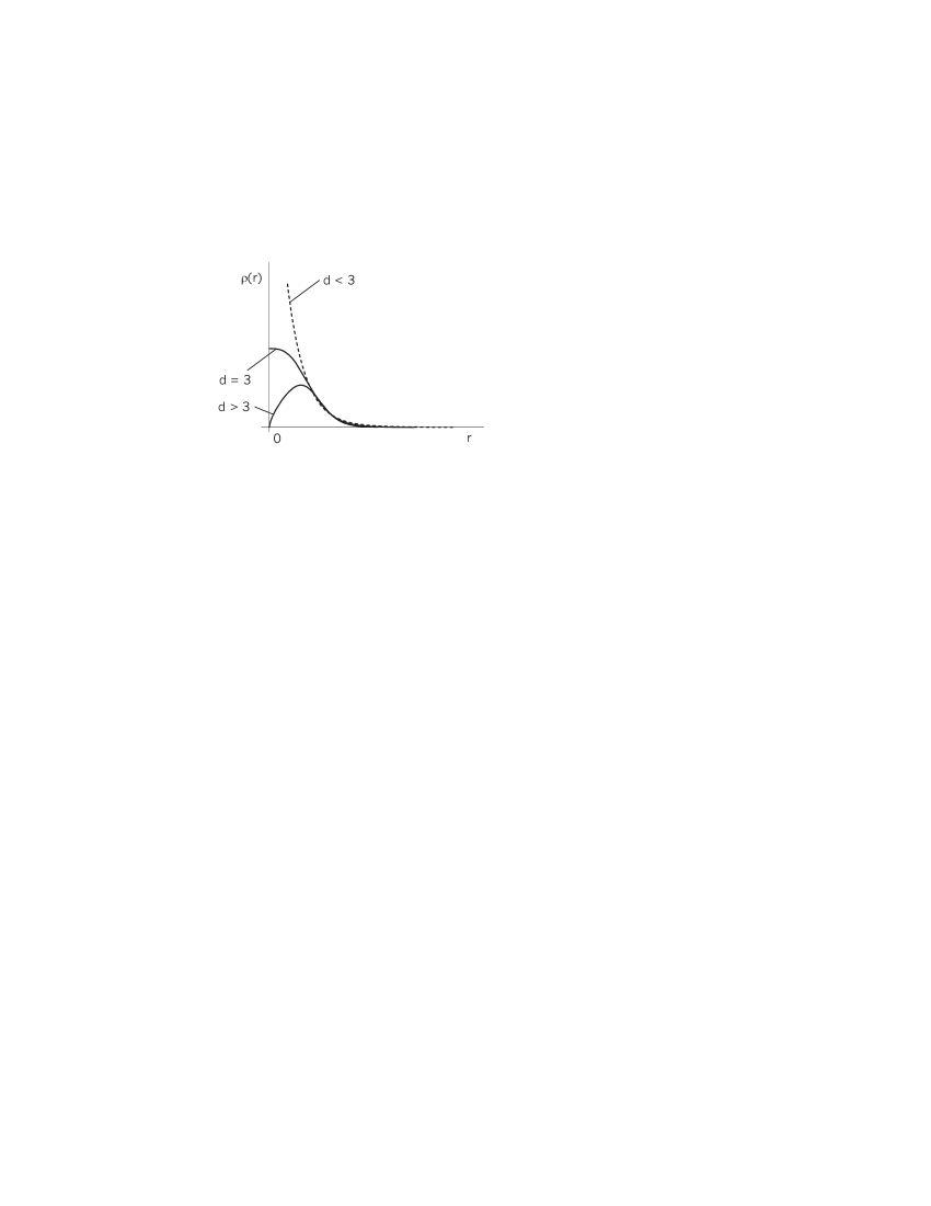
and investigate the behavior of the density as a radial function. For the single fluid the density is regular and positive at zero when the parameter $d$ (see the previous section) is equal to $d^{*}=D-d_{I_{(1)}}-2$. In this case the brane submanifold fills the total manifold (2.2) except $R_{*}\times S^{d_{0}}$.When $d<d^{*}$ the density is infinite at zero.

For multi-component fluid all densities are finite at $r=0$, if (and only if)

$$\sum_{s=1}^{m}\frac{1}{D-d_{I_{s}}-2}\geq\frac{1}{d}.$$ (4.4)

Moreover, all ρ(s)​(0)>0superscriptπœŒπ‘ 00\rho^{(s)}(0)>0 when the equality in (4.4) takes place.

Refer to caption
Figure 1: The variants of behavior of $\rho(r)$ for $M2\cap M2$ intersection

As an example we consider simulation by MCAF of intersecting $M2\cap M5$, $M2\cap M2$, $M5\cap M5$ configurations in $D=11$ supergravity. The metric for all cases reads:

$\displaystyle{}ds^{2}=J_{0}\Biggl{[}\displaystyle\frac{\mathstrut dr^{2}}{1-2\mu/r}+r^{2}d\Omega^{2}_{d_{0}}-{(H_{(I)})}^{-1}{(H_{(II)})}^{-1}\biggl{\{}\left(1-\frac{2\mu}{r}\right)dt^{2}+h^{[2]}_{m_{2}n_{2}}dy^{m_{2}}dy^{n_{2}}\biggr{\}}$
$\displaystyle+H_{(I)}^{-1}h^{[3]}_{m_{3}n_{3}}dy^{m_{3}}dy^{n_{3}}+H_{(II)}^{-1}h^{[4]}_{m_{4}n_{4}}dy^{m_{4}}dy^{n_{4}}+h^{[5]}_{m_{5}n_{5}}dy^{m_{5}}dy^{n_{5}}\Biggr{]},$ (4.5)

where we can express the factor $J_{0}=H_{(I)}^{2/(D-d_{I_{(I)}}-2)}H_{(II)}^{2/(D-d_{I_{(II)}}-2)}$; the first brane world-volume is $M_{1}\times M_{2}\times M_{3}$, the second one is $M_{1}\times M_{2}\times M_{4}$.

$a).$ For MCAF, corresponding to intersecting of $M2$ (with index $I$ in (4)) and $M5$ (with index $II$) branes the dimensions are following $d_{1}=d_{2}=d_{3}=1,\ d_{4}=4$ and $J_{0}=H_{(I)}^{1/3}H_{(II)}^{2/3}$.

The densities $\rho^{(I)},\ \rho^{(II)}$ are infinite at zero when $d=1$ and for $d=2$ they are finite: $\rho^{(I)}(0)=(P_{I}+2\mu)/H_{I}^{4/3}H_{II}^{2/3}$, $\rho^{(II)}(0)=(P_{II}+2\mu)/H_{II}^{5/3}H_{I}^{1/3}$. It is interesting to note that in the extremal limit $\mu\rightarrow 0$ $\rho^{(I)}(0)=\rho^{(II)}(0)$.

$b).$ For MCAF equivalent to two electrical $M2$ branes intersecting on the time manifold we get $d_{3}=d_{4}=2,\ d_{2}=0$. Here $J_{0}=H_{(I)}^{1/3}H_{(II)}^{1/3}$.

The variants of behavior of the densities are presented on Figure 1. When $d=3$ both functions are regular and positive at zero (the middle branch).

$c).$ For two $M5$ branes the dimension of intersection is 4 and $d_{0}=d_{3}=d_{4}=2,\ d_{2}=3,\ d_{5}=0$ and $J_{0}=H_{(I)}^{2/3}H_{(II)}^{2/3}$. The only possibility here is $d=1$ and the fluid densities are infinite at zero.

5 Physical parameters

5.1 Gravitational mass and post-Newtonian parameters

Here for simplicity we put $d_{0}=2\ (d=1)$. Consider the 4-dimensional space-time section of the metric (3.5). Introducing a new radial variable by the relation

$$r=R\left(1+\frac{\mu}{2R}\right)^{2},$$ (5.1)

we rewrite the 4-section in the following form:

d​s(4)2=gμ​μ′(4)​d​xμ​d​xΞΌβ€²=(∏s=1mHsβˆ’2​νs2​U(s)​0)​[βˆ’(1βˆ’ΞΌ/2​R1+ΞΌ/2​R)2​(∏s=1mHsβˆ’2​νs2)​d​t2+(1+ΞΌ2​R)4​δi​j​d​xi​d​xj],𝑑superscriptsubscript𝑠42subscriptsuperscript𝑔4πœ‡superscriptπœ‡β€²π‘‘superscriptπ‘₯πœ‡π‘‘superscriptπ‘₯superscriptπœ‡β€²superscriptsubscriptproduct𝑠1π‘šsuperscriptsubscript𝐻𝑠2superscriptsubscriptπœˆπ‘ 2superscriptπ‘ˆπ‘ 0delimited-[]superscript1πœ‡2𝑅1πœ‡2𝑅2superscriptsubscriptproduct𝑠1π‘šsuperscriptsubscript𝐻𝑠2superscriptsubscriptπœˆπ‘ 2𝑑superscript𝑑2superscript1πœ‡2𝑅4subscript𝛿𝑖𝑗𝑑superscriptπ‘₯𝑖𝑑superscriptπ‘₯𝑗\displaystyle{}ds_{(4)}^{2}=g^{(4)}_{\mu\mu^{\prime}}dx^{\mu}dx^{\mu^{\prime}}=\left(\prod_{s=1}^{m}H_{s}^{-2\nu_{s}^{2}U^{(s)0}}\right)\left[-\left(\frac{1-{\mu}/{2R}}{1+{\mu}/{2R}}\right)^{2}\left(\prod_{s=1}^{m}H_{s}^{-2\nu_{s}^{2}}\right)dt^{2}+\left(1+\frac{\mu}{2R}\right)^{4}\delta_{ij}dx^{i}dx^{j}\right], (5.2)

$i,j=1,2,3$. Here $R^{2}=\delta_{ij}x^{i}x^{j}$.

The post-Newtonian (Eddington) parameters are defined by the well-known relations

$\displaystyle g^{(4)}_{00}$ $\displaystyle=$ $\displaystyle-(1-2V+2\beta V^{2})+O(V^{3}),$ (5.3)
$\displaystyle g^{(4)}_{ij}$ $\displaystyle=$ $\displaystyle\delta_{ij}(1+2\gamma V)+O(V^{2}),$ (5.4)

$i,j=1,2,3$. Here $V={GM}/{R}$ is the Newtonian potential, $M$ is the gravitational mass and $G$ is the gravitational constant. From (5.2)-(5.4) we obtain:

G​M=ΞΌ+βˆ‘s=1mΞ½s2​Ps​(1+U(s)​0),πΊπ‘€πœ‡superscriptsubscript𝑠1π‘šsuperscriptsubscriptπœˆπ‘ 2subscript𝑃𝑠1superscriptπ‘ˆπ‘ 0GM=\mu+\sum_{s=1}^{m}\nu_{s}^{2}P_{s}(1+U^{(s)0}), (5.5)

and

$\displaystyle\beta-1$ $\displaystyle=$ 12​(G​M)2β€‹βˆ‘s=1mΞ½s2​Ps​(Ps+2​μ)​(1+U(s)​0),12superscript𝐺𝑀2superscriptsubscript𝑠1π‘šsuperscriptsubscriptπœˆπ‘ 2subscript𝑃𝑠subscript𝑃𝑠2πœ‡1superscriptπ‘ˆπ‘ 0\displaystyle\frac{1}{2(GM)^{2}}\sum_{s=1}^{m}\ \nu_{s}^{2}P_{s}(P_{s}+2\mu)(1+U^{(s)0}), (5.6)
$\displaystyle\gamma-1$ $\displaystyle=$ βˆ’1G​Mβ€‹βˆ‘s=1mΞ½s2​Ps​(1+2​U(s)​0).1𝐺𝑀superscriptsubscript𝑠1π‘šsuperscriptsubscriptπœˆπ‘ 2subscript𝑃𝑠12superscriptπ‘ˆπ‘ 0\displaystyle-\frac{1}{GM}\sum_{s=1}^{m}\ \nu_{s}^{2}P_{s}(1+2U^{(s)0}). (5.7)

For fixed vector U(s)superscriptπ‘ˆπ‘ U^{(s)} the parameter $\beta-1$ is proportional to the ratio of two physical parameters: the anisotropic fluid density parameter $A_{s}$ (see (B.15)), and the gravitational radius squared $(GM)^{2}$.

5.2 The Hawking temperature

The Hawking temperature of a black hole may be calculated using the relation from [8] and has the following form:

TH=d4​π​(2​μ)1/dβ€‹βˆs=1m(2​μ2​μ+Ps)Ξ½s2.subscript𝑇𝐻𝑑4πœ‹superscript2πœ‡1𝑑superscriptsubscriptproduct𝑠1π‘šsuperscript2πœ‡2πœ‡subscript𝑃𝑠superscriptsubscriptπœˆπ‘ 2T_{H}=\frac{d}{4\pi(2\mu)^{1/d}}\prod_{s=1}^{m}\left(\frac{2\mu}{2\mu+P_{s}}\right)^{\nu_{s}^{2}}. (5.8)

6 Conclusions

Here we have obtained a family of spherically symmetric solutions with horizon in the model with multi-component anisotropic fluid with the equations of state (2.8) and the conditions (3.1) imposed. The metric of any solution contains $(n-1)$ Ricci-flat β€œinternal” space metrics. For certain equations of state (with $p_{i}=\pm\rho$) the metric of the solution may coincide with the metric of intersecting black branes (in a model with antisymmetric forms without dilatons). Here the examples of simulating of intersecting $M2$ and $M5$ black branes in $D=11$ supergravity are considered.

We have also calculated the post-Newtonian parameters $\beta$ and $\gamma$ corresponding to the 4-dimensional section of the metric. The parameter $\beta-1$ is written in terms of ratios of the physical parameters: the anisotropic fluid parameter $|A_{s}|$ and the gravitational radius squared $(GM)^{2}$. An open problem is to generalize the formalism to the case when dilaton scalar fields are added into consideration.

Acknowlegments

This work was supported in part by the Russian Ministry of Science and Technology, Russian Foundation for Basic Research (Grant 01-02-17312), project SEE and DFG project (436 RUS 113/678/0-1(R)).

V.D.I. and V.N.M. thank Prof. Dr. H. Dehnen and his colleagues at the University of Konstanz for their hospitality.

Appendix

A Lagrange representation

The ”conservation law” equation (2.7) may be written, due to relations (2.3) and (2.6) in the following form:

ρ^Λ™(s)+βˆ‘i=0ndi​Xi˙​(ρ^(s)+p^i(s))=0.superscriptΛ™^πœŒπ‘ superscriptsubscript𝑖0𝑛subscript𝑑𝑖˙superscript𝑋𝑖superscript^πœŒπ‘ subscriptsuperscript^𝑝𝑠𝑖0\dot{\hat{\rho}}^{(s)}+\sum_{i=0}^{n}d_{i}\dot{X^{i}}({\hat{\rho}}^{(s)}+{\hat{p}}^{(s)}_{i})=0. (A.1)

Using the equation of state (2.8) we get

ρ^(s)=βˆ’As​e2​Ui(s)​Xiβˆ’2​γ0,superscript^πœŒπ‘ subscript𝐴𝑠superscript𝑒2subscriptsuperscriptπ‘ˆπ‘ π‘–superscript𝑋𝑖2subscript𝛾0{\hat{\rho}}^{(s)}=-A_{s}e^{2U^{(s)}_{i}X^{i}-2\gamma_{0}}, (A.2)

where $\gamma_{0}(X)=\sum\limits_{i=0}^{n}d_{i}X^{i}$, and $A_{s}$ are constants.

The Einstein equations (2.1) with the relations (2.8) and (A.2) imposed are equivalent to the Lagrange equations for the Lagrangian

$$L=\frac{1}{2}e^{-\gamma+\gamma_{0}(X)}G_{ij}\dot{X}^{i}\dot{X}^{j}-e^{\gamma-\gamma_{0}(X)}V,$$ (A.3)

where

V=12​d0​(d0βˆ’1)​e2​Ui(0)​Xi+βˆ‘s=1mAs​e2​Ui(s)​Xi=βˆ‘s=0mAs​e2​Ui(s)​Xi,𝑉12subscript𝑑0subscript𝑑01superscript𝑒2subscriptsuperscriptπ‘ˆ0𝑖superscript𝑋𝑖superscriptsubscript𝑠1π‘šsubscript𝐴𝑠superscript𝑒2subscriptsuperscriptπ‘ˆπ‘ π‘–superscript𝑋𝑖superscriptsubscript𝑠0π‘šsubscript𝐴𝑠superscript𝑒2subscriptsuperscriptπ‘ˆπ‘ π‘–superscript𝑋𝑖V=\frac{1}{2}d_{0}(d_{0}-1)e^{2U^{(0)}_{i}X^{i}}+\sum_{s=1}^{m}A_{s}e^{2U^{(s)}_{i}X^{i}}=\sum_{s=0}^{m}A_{s}e^{2U^{(s)}_{i}X^{i}}, (A.4)

is the potential and the components of the minisupermetric $G_{ij}$ are defined in (3.3).

$$U^{(0)}_{i}X^{i}=-X^{0}+\gamma_{0}(X),\qquad U^{(0)}_{i}=-\delta^{0}_{i}+d_{i},\qquad A_{0}=\frac{1}{2}d_{0}(d_{0}-1),$$ (A.5)

$i=0,\ldots,n$.

For $\gamma=\gamma_{0}(X)$, i.e. when the harmonic time gauge is considered, we get the set of Lagrange equations for the Lagrangian

$$L=\frac{1}{2}G_{ij}\dot{X}^{i}\dot{X}^{j}-V,$$ (A.6)

with the zero-energy constraint imposed

$$E=\frac{1}{2}G_{ij}\dot{X}^{i}\dot{X}^{j}+V=0.$$ (A.7)

It follows from the restriction U0(s)=0subscriptsuperscriptπ‘ˆπ‘ 00U^{(s)}_{0}=0 that

(U(0),U(s))≑Ui(0)​Gi​j​Uj(s)=0.superscriptπ‘ˆ0superscriptπ‘ˆπ‘ subscriptsuperscriptπ‘ˆ0𝑖superscript𝐺𝑖𝑗subscriptsuperscriptπ‘ˆπ‘ π‘—0(U^{(0)},{U^{(s)}})\equiv U^{(0)}_{i}G^{ij}U^{(s)}_{j}=0. (A.8)

Indeed, the contravariant components $U^{(0)i}=G^{ij}U^{(0)}_{j}$ are the following ones

$$U^{(0)i}=-\frac{\delta_{0}^{i}}{d_{0}}.$$ (A.9)

Then we get (U(0),U(s))=U(0)​i​Ui(s)=βˆ’U0(s)/d0=0superscriptπ‘ˆ0superscriptπ‘ˆπ‘ superscriptπ‘ˆ0𝑖subscriptsuperscriptπ‘ˆπ‘ π‘–subscriptsuperscriptπ‘ˆπ‘ 0subscript𝑑00(U^{(0)},U^{(s)})=U^{(0)i}U^{(s)}_{i}=-U^{(s)}_{0}/d_{0}=0. In what follows we also use the formula

$$\frac{1}{\nu_{0}^{2}}=(U^{(0)},U^{(0)})=\frac{1}{d_{0}}-1<0,$$ (A.10)

for $d_{0}>1$.

In what follows we will make the following assumption on indices: $s=1,\ldots,m$ and $\alpha=0,\ldots,m$.

B General spherically symmetric and cosmological-type solutions

When the orthogonality relations (A.8) and $3^{o}$ of (3.1) are satisfied the Euler-Lagrange equations for the Lagrangian (A.6) with the potential (A.4) have the following solutions (see relations from [7] adopted for our case):

$$X^{i}(u)=-\sum_{\alpha=0}^{m}\frac{U^{(\alpha)i}}{(U^{(\alpha)},U^{(\alpha)})}\ln|f_{\alpha}(u-u_{\alpha})|+c^{i}u+\bar{c}^{i},$$ (B.1)

where $u_{\alpha}$ ($\alpha=0,\ldots,m$) are integration constants; and vectors $c=(c^{i})$ and $\bar{c}=(\bar{c}^{i})$ are orthogonal to the $U^{(\alpha)}=(U^{(\alpha)i})$, i.e. they satisfy the linear constraint relations

$\displaystyle U^{(0)}(c)=U^{(0)}_{i}c^{i}=-c^{0}+\sum_{j=0}^{n}d_{j}c^{j}=0,$ (B.2)
$\displaystyle U^{(0)}(\bar{c})=U^{(0)}_{i}\bar{c}^{i}=-\bar{c}^{0}+\sum_{j=0}^{n}d_{j}\bar{c}^{j}=0,$ (B.3)
U(s)​(c)=Ui(s)​ci=0,superscriptπ‘ˆπ‘ π‘subscriptsuperscriptπ‘ˆπ‘ π‘–superscript𝑐𝑖0\displaystyle U^{(s)}(c)=U^{(s)}_{i}c^{i}=0, (B.4)
U(s)​(cΒ―)=Ui(s)​cΒ―i=0.superscriptπ‘ˆπ‘ Β―π‘subscriptsuperscriptπ‘ˆπ‘ π‘–superscript¯𝑐𝑖0\displaystyle U^{(s)}(\bar{c})=U^{(s)}_{i}\bar{c}^{i}=0. (B.5)

Here

fα​(Ο„)=Rα​sh(Cα​τ)CΞ±,CΞ±β‰ 0,Ξ·Ξ±=+1,Rα​ch(Cα​τ)CΞ±,CΞ±>0,Ξ·Ξ±=βˆ’1,Rα​τ,CΞ±=0,Ξ·Ξ±=+1,subscriptπ‘“π›Όπœabsentsubscript𝑅𝛼shsubscriptπΆπ›Όπœsubscript𝐢𝛼subscript𝐢𝛼0subscriptπœ‚π›Ό1missing-subexpressionsubscript𝑅𝛼chsubscriptπΆπ›Όπœsubscript𝐢𝛼subscript𝐢𝛼0subscriptπœ‚π›Ό1missing-subexpressionmissing-subexpressionmissing-subexpressionmissing-subexpressionmissing-subexpressionsubscriptπ‘…π›Όπœsubscript𝐢𝛼0subscriptπœ‚π›Ό1\begin{array}[]{rlll}f_{\alpha}(\tau)=&R_{\alpha}\displaystyle\frac{\mathstrut\mathop{\rm sh}\nolimits(\displaystyle\sqrt{\mathstrut C_{\alpha}}\tau)}{\displaystyle\sqrt{\mathstrut C_{\alpha}}},&C_{\alpha}\neq 0,&\eta_{\alpha}=+1,\\ &R_{\alpha}\displaystyle\frac{\mathstrut\mathop{\rm ch}\nolimits(\displaystyle\sqrt{\mathstrut C_{\alpha}}\tau)}{\displaystyle\sqrt{\mathstrut C_{\alpha}}},&C_{\alpha}>0,&\eta_{\alpha}=-1,\\ \\ &R_{\alpha}\tau,&C_{\alpha}=0,&\eta_{\alpha}=+1,\end{array} (B.6)

$R_{\alpha}=\sqrt{2|A_{\alpha}/\nu_{\alpha}^{2}|}$, $\eta_{\alpha}=-\mathop{\rm sign}\nolimits(A_{\alpha}/\nu_{\alpha}^{2})$; and parameters $\nu_{\alpha}$ are defined in (3.10) and (A.10), $\alpha=0,\ldots,m$.

The zero-energy constraint, corresponding to the solution (B.1) reads

$$E=\frac{1}{2}\sum_{\alpha=0}^{m}\frac{C_{\alpha}}{(U^{(\alpha)},U^{(\alpha)})}+\frac{1}{2}G_{ij}c^{i}c^{j}=0.$$ (B.7)

From (B.1) we get the following relation for the metric (see also (3.3), (A.9) and (A.10))

g=e2​c0​u+2​cΒ―0​(∏α=0mfΞ±βˆ’2​ν2​U(Ξ±)​0)​{d​uβŠ—d​u+f02​h[0]}+βˆ‘iβ‰ 0e2​ci​u+2​cΒ―i​(∏α=0mfΞ±βˆ’2​ν2​U(Ξ±)​i)​h[i],𝑔superscripte2superscript𝑐0𝑒2superscript¯𝑐0superscriptsubscriptproduct𝛼0π‘šsuperscriptsubscript𝑓𝛼2superscript𝜈2superscriptπ‘ˆπ›Ό0tensor-product𝑑𝑒𝑑𝑒superscriptsubscript𝑓02superscriptβ„Ždelimited-[]0subscript𝑖0superscripte2superscript𝑐𝑖𝑒2superscript¯𝑐𝑖superscriptsubscriptproduct𝛼0π‘šsuperscriptsubscript𝑓𝛼2superscript𝜈2superscriptπ‘ˆπ›Όπ‘–superscriptβ„Ždelimited-[]𝑖\begin{array}[]{l}g={\,\rm e}^{2c^{0}u+2\bar{c}^{0}}\ \left(\prod\limits_{\alpha=0}^{m}f_{\alpha}^{{}^{\mathstrut-2\nu^{2}U^{(\alpha)0}}}\right)\biggl{\{}\ du\otimes du+f_{0}^{2}\ h^{[0]}\biggr{\}}+\sum\limits_{i\neq 0}\ {\,\rm e}^{2c^{i}u+2\bar{c}^{i}}\ \left(\prod\limits_{\alpha=0}^{m}f_{\alpha}^{{}^{\mathstrut-2\nu^{2}U^{(\alpha)i}}}\right)\ h^{[i]},\end{array} (B.8)

where $f_{\alpha}=f_{\alpha}(u-u_{\alpha})$ (here we use the relations $d_{i}U^{i}+\frac{U_{0}}{d_{0}}=U^{0}$ and (A.10)).

Solutions with horizon. For integration constants we put

$\displaystyle\bar{c}^{i}$ $\displaystyle=$ $\displaystyle 0,$ (B.9)
$\displaystyle c^{i}$ $\displaystyle=$ $\displaystyle\bar{\mu}\sum_{\alpha=0}^{m}\frac{U^{{(\alpha)}i}}{(U^{(\alpha)},U^{(\alpha)})}-\bar{\mu}\delta^{i}_{1},$ (B.10)
$\displaystyle C_{\alpha}$ $\displaystyle=$ $\displaystyle\bar{\mu}^{2},$ (B.11)

where $\bar{\mu}>0$, $\alpha=0,\ldots,m$.

We also introduce new radial variable $r=r(u)$ by relations

$$\exp(-2\bar{\mu}u)=1-\frac{2\mu}{r^{d}},\quad\mu=\bar{\mu}/d>0,\quad d=d_{0}-1,$$ (B.12)

and put $u_{0}=0$; $u_{s}<0$, $A_{s}<0,\ s=1,\ldots,m$,

2​|As|μ¯​νs​shΞ²s=1,Ξ²s≑μ¯​|us|.formulae-sequence2subscriptπ΄π‘ Β―πœ‡subscriptπœˆπ‘ shsubscript𝛽𝑠1subscriptπ›½π‘ Β―πœ‡subscript𝑒𝑠\frac{\sqrt{2|A_{s}|}}{\bar{\mu}\nu_{s}}\mathop{\rm sh}\nolimits\beta_{s}=1,\quad\beta_{s}\equiv\bar{\mu}|u_{s}|. (B.13)

Now the parameter $P_{s}$ may be introduced ($P_{s}>0$) by the following relation:

$$\frac{\mu}{\mathop{\rm sh}\nolimits\beta_{s}}=P_{s}e^{\beta_{s}}=\sqrt{P_{s}(P_{s}+2\mu)},$$ (B.14)

and, hence,

βˆ’As=12​νs2​d2​Ps​(Ps+2​μ),subscript𝐴𝑠12superscriptsubscriptπœˆπ‘ 2superscript𝑑2subscript𝑃𝑠subscript𝑃𝑠2πœ‡-A_{s}=\frac{1}{2}\nu_{s}^{2}d^{2}P_{s}(P_{s}+2\mu), (B.15)

see (A.2). The relations of the Appendix imply the formulae (3.5), (3.6) for the solution from Section 3.

References

  • [1] V.D. Ivashchuk and V.N. Melnikov, Class. Quantum Grav. 18 R87-R152 (2001); hep-th/0110274.
  • [2] V.D. Ivashchuk and V.N. Melnikov, Grav. & Cosmol., 6, 27-40 (2000); hep-th/9910041.
  • [3] K.A. Bronnikov, V.D. Ivashchuk and V.N. Melnikov Grav. & Cosmol. 3, 203-212 (1997); gr-qc/9710054.
  • [4] V.D Ivashchuk, V.N. Melnikov, J. Math. Phys. 39, 2866–2889 (1998); hep-th/9708157.
  • [5] V.D. Ivashchuk, V.N. Melnikov and A.I. Zhuk, Nuovo Cim. B 104, 5, 575-581 (1989).
  • [6] V.D. Ivashchuk and V.N. Melnikov, Int. J. Mod. Phys. D 3, 4, 795-811 (1994); gr-qc/ 9403063.
  • [7] V.R. Gavrilov, V.D. Ivashchuk, V.N. Melnikov, J. Math. Phys 36, 5829–5847 (1995).
  • [8] J.W. York, Phys. Rev. D 31, 775 (1985).
  • [9] K.S. Stelle, hep-th/9701088.
  • [10] M. Cvetic and A. Tseytlin, Nucl. Phys. B 478, 181-198 (1996); hep-th/9606033.
  • [11] I.Ya. Aref’eva, M.G. Ivanov and I.V. Volovich, Phys. Lett. B 406, 44-48 (1997); hep-th/9702079.
  • [12] V.D. Ivashchuk, V.N. Melnikov and A.B. Selivanov, Grav. Cosmol. 7 4(12), (2001); gr-qc/0205103.

List of captions for illustrations

Figure 1. The variants of behavior of $\rho(r)$ for $M2\cap M2$ intersection.