Intersecting D3-branes and Holography

Neil R. Constable$\,{}^{a}$, Johanna Erdmenger$\,{}^{b}$, Zachary Guralnik$\,{}^{b}$ and Ingo Kirsch$\,{}^{b}$

^a Center for Theoretical Physics and Laboratory for Nuclear Science

Massachusetts Institute of Technology

77 Massachusetts Avenue

Cambridge, MA 02139, USA

^b Institut für Physik

Humboldt-Universität zu Berlin

Invalidenstraße 110

D-10115 Berlin, Germany

Abstract

We study a defect conformal field theory describing D3-branes intersecting over two space-time dimensions. This theory admits an exact Lagrangian description which includes both two- and four-dimensional degrees of freedom, has $(4,4)$ supersymmetry and is invariant under global conformal transformations. Both two- and four-dimensional contributions to the action are conveniently obtained in a two-dimensional $(2,2)$ superspace. In a suitable limit, the theory has a dual description in terms of a probe D3-brane wrapping an $AdS_{3}\times S^{1}$ slice of $AdS_{5}\times S^{5}$. We consider the AdS/CFT dictionary for this set-up. In particular we find classical probe fluctuations corresponding to the holomorphic curve $wy=c\alpha^{\prime}$. These fluctuations are dual to defect fields containing massless two-dimensional scalars which parameterize the classical Higgs branch, but do not correspond to states in the Hilbert space of the CFT. We also identify probe fluctuations which are dual to BPS superconformal primary operators and to their descendants. A non-renormalization theorem is conjectured for the correlators of these operators, and verified to order $g^{2}$.

1 Introduction and summary

The general problem of introducing a spatial defect into a conformal field theory has been studied in several contexts [1, 2]. Within string theory such defect conformal field theories arise in various brane constructions. They were first studied in this context as matrix model descriptions of compactified NS5-branes [3] and more generally as effective field theories describing various D-brane intersections [4, 5]. More recently, an extension of AdS/CFT duality [6] was conjectured in which an $AdS_{5}\times S^{5}$ background is probed with a D5-brane wrapping an $AdS_{4}\times S^{2}$ submanifold. This configuration has been conjectured to be dual to a four-dimensional conformal field theory coupled to a codimension one defect [7]. This defect conformal field theory describes the decoupling limit of the D3-D5 intersection, and consists of the ${\cal N}=4,d=4$ super Yang-Mills theory coupled to an ${\cal N}=4,d=3$ hypermultiplet localized at the defect. The open string modes with both endpoints on the D5-brane decouple in the infrared. Holographic duality can be viewed as acting twice: The ${\cal N}=4,d=4$ super Yang-Mills degrees of freedom are dual to closed strings in $AdS_{5}\times S^{5}$, while the defect hypermultiplet degrees of freedom are dual to open strings with endpoints on the probe D5-brane wrapping $AdS_{4}\times S^{2}$. In [8], the action of the model was written down, and the chiral primaries localized on the defect were identified along with the dual fluctuations on the $AdS_{4}$ brane. In [9], the action was written compactly in an ${\cal N}=2,d=3$ superspace, and field theoretic arguments for quantum conformal invariance were given. The supersymmetry of the $AdS_{4}\times S^{2}$ embedding was demonstrated in [10]. Gravitational aspects of this set-up were discussed in [11, 12, 13]. The Penrose limit of this background was studied in [10, 14], wherein a map between defect operators with large $R$-charge and open strings on a D3-brane in a plane wave background was constructed. Moreover, two-dimensional conformal field theories with a one-dimensional defect dual to $AdS_{2}$ branes in $AdS_{3}$ have recently been studied in [15, 16]. In [17, 18] spacetime filling D7-branes were added to the $AdS_{5}/{\rm CFT}_{4}$ correspondence in order to study flavors in supersymmetric extensions of QCD. Similarly the supergravity solution for the D2/D6 intersection, dual to 2+1-dimensional Yang-Mills with flavor, was obtained in [19]. RG flows related to defect conformal field theories were discussed in [20]. Finally, defect CFT’s were discussed in connection with the phenomenon of supertubes in [21].

In this paper we consider a defect conformal field theory which describes the low energy dynamics of intersecting D3-branes. This system consists of a stack of D3-branes spanning the $0123$ directions and an orthogonal stack spanning the $0145$ directions such that eight supercharges are preserved, realizing a a $(4,4)$ supersymmetry on the common $1+1$ dimensional world volume. This theory exhibits interesting properties which did not arise for the D3-D5 intersection. Unlike the D3-D5 intersection, open strings on both stacks of branes remain coupled as $\alpha^{\prime}\rightarrow 0$. The resulting theory is described by a linear sigma model on two intersecting world volumes. The classical Higgs branch of this theory has an interpretation as a smooth resolution of the intersection to the holomorphic curve $wy\sim c\alpha^{\prime}$, where $w=X^{2}+iX^{3}$ and $y=X^{4}+iX^{5}$. However, due to the two-dimensional nature of the fields which parameterize these curves the quantum vacuum spreads out over the entire classical Higgs branch.

As a result of the spreading over the Higgs branch, it has been argued that a fully localized supergravity solution for this D3-brane intersection does not exist [22, 23, 24]. Obtaining a closed string description of this defect CFT would therefore seem to be difficult. From the point of view of the linear sigma model description, a holographic equivalence with a closed string background would seem to require a target space with a singular boundary. Nevertheless, there is a limit in which a holographic duality be found relating fluctuations in an $AdS$ background to operators in the linear sigma model. One simply takes the number of D3-branes, $N$, in the first stack to infinity, keeping $g_{s}N$ and the number of D3-branes in the second stack, $N^{\prime}$, fixed. In this limit, the ’t Hooft coupling of the gauge theory on the second stack, $\lambda^{\prime}=g_{s}N^{\prime}$, vanishes. Thus the open strings with all endpoints on the second stack decouple, and one is left with a four-dimensional CFT with a codimension two defect. The defect breaks half of the original $\mathcal{N}=4$, $d=4$ supersymmetry, leaving eight real supercharges realizing a two-dimensional $(4,4)$ supersymmetry algebra. The conformal symmetry of the theory is a global $SL(2,R)\times SL(2,R)$, corresponding to a subgroup of the four-dimensional conformal symmetries. The degrees of freedom at the impurity are a $(4,4)$ hypermultiplet arising from the open strings connecting the orthogonal stacks of D3-branes.

In the limit described above, the holographic dual is obtained by focusing on the near horizon region for the first stack of D3-branes, while treating the second stack as a probe. The result is an $AdS_{5}\times S^{5}$ background with $N^{\prime}$ probe D3-branes wrapping an $AdS_{3}\times S^{1}$ subspace. This embedding was shown to be supersymmetric in [10]. We will demonstrate below that there is a one complex parameter family of such embeddings, corresponding to the holomorphic curves $wy\sim c$, all of which preserve a set of isometries corresponding to the super-conformal group. In the spirit of [7], holographic duality is conjectured to act “twice”. First there is the standard AdS/CFT duality relating closed strings in $AdS_{5}\times S^{5}$ to operators in ${\cal N}=4$ super Yang-Mills theory. Second, there is a duality relating open strings on the probe D$3^{\prime}$ wrapping $AdS_{3}\times S^{1}$ to operators localized on the $1+1$ dimensional defect.

One of the original motivations to search for holographic dualities for defect conformal field theories [7] is that such a duality might imply the localization of gravity on branes in string theory. In the context of a brane wrapping an $AdS_{3}$ geometry embedded inside $AdS_{5}$, localization of gravity would indicate the existence of a Virasoro algebra in the dual CFT, through a Brown-Henneaux mechanism [25]. We do not find any evidence for the existence of a Virasoro algebra in the conformal field theory. Although this theory has a $(4,4)$ superconformal algebra, only the finite part of the algebra is realized in any obvious way. Roughly speaking, the $(4,4)$ superconformal algebra is the common intersection of two ${\cal N}=4,d=4$ superconformal algebras, both of which are finite. The even part of the superconformal group is $SL(2,R)\times SL(2,R)\times SU(2)_{L}\times SU(2)_{R}\times U(1)$, which is also realized as an isometry of the $AdS_{5}$ background which preserves the probe embedding. Enhancement to the usual infinite dimensional algebra would require the existence of a decoupled two-dimensional sector. Correctly addressing this issue would require going beyond the probe limit and studying the back reaction of the D$3^{\prime}$-branes on the $AdS_{5}\times S^{5}$ geometry as well as gaining a deeper understanding of the dynamics of the defect CFT.

The action for the D3-D3 intersection is most easily and elegantly constructed in $(2,2)$ superspace. Although it may seem unusual to write the ${\cal N}=4,d=4$ components of the action in $(2,2)$ superspace, this is actually quite natural because the four-dimensional supersymmetries are broken by couplings to the defect hypermultiplet. In writing this action, we will not take the limit which decouples one stack of D3-branes. With the help of the manifest chirality of $(2,2)$ superspace we are able to find an argument for the absence of quantum corrections to the combined 2d/4d actions, which implies that the theory remains conformal upon quantization. Although this theory has two-dimensional fields coupled to gauge fields, the gauge couplings couplings are exactly marginal due to the four-dimensional nature of the gauge fields.

We give a detailed dictionary between Kaluza-Klein fluctuations on the probe D3-brane and operators localized on the defect. Of particular interest will be a certain subset of the fluctuations which describe the embedding of the probe inside $AdS_{5}$. This subset is dual to operators containing defect scalar fields, which appear without any derivative or vertex operator structure. Due to strong infrared effects in two dimensions, these fields are not conformal fields associated to states in the Hilbert space. From the point of view of the probe-supergravity system, there is at first sight nothing unusual about these fluctuations. However upon applying the usual $AdS_{3}$/CFT₂ rules to compute the dual two-point correlator, one finds identically zero due to extra surface terms in the probe action. Thus there is no clear interpretation of these fluctuations as sources for the generating function of the CFT. We shall find however that the bottom of the Kaluza-Klein tower for these fluctuations (with appropriate boundary conditions) parameterizes the aforementioned holomorphic embedding of the probe inside $AdS_{5}$. While the interpretation of this fluctuation as a source is unclear, it nevertheless labels points on the classical Higgs branch. Since the infrared dynamics of two dimensions implies that the vacuum is spread out over the entire Higgs branch, one should in principle sum over holomorphic embeddings when performing computations in the $AdS$ background.

The fluctuations of the probe $S^{1}$ embedding inside $S^{5}$ satisfy the Breitenlohner-Freedman bound despite the lack of topological stability. These fluctuations are dual to a multiplet of scalar operators with defect fermion pairs which we identify with BPS superconformal primaries localized at the intersection. We also find fluctuations of the probe embedding inside $AdS_{5}$ which are dual to descendants of these operators. Remarkably, the AdS computation of the corresponding correlators, which is valid for large ’t Hooft coupling $\lambda$, shows no dependence on $\lambda$. We also study perturbative quantum corrections to the two-point function of the BPS primary operators and find that such corrections are absent at order $g_{YM}^{2}$. Together with the $AdS$ strong coupling result, this suggests the existence of a non-renormalization theorem.

The paper is organized as follows. In section 2 we present the D3-brane setup, its near horizon isometries and the superconformal algebra. In section 3 we obtain the spectrum of low-energy fluctuations about the probe geometry. In section 4 we show that the n-point functions associated with these fluctuations are independent of the ’t Hooft coupling, at least when the ’t Hooft coupling is large. Moreover we show that the classical action for probe fluctuations dual operators parameterizing the classical Higgs branch does correspond to a power law two-point function. In section 5 we study the field theory associated with the D3-brane intersection. We obtain the action using $(2,2)$ superspace for both the defect and four-dimensional components. In section 6 we derive the fluctuation-operator dictionary for the conjectured AdS/CFT correspondence. In section 7 we demonstrate that two-point functions of the BPS primary operators identified in section 6 do not receive any radiative corrections to order $g^{2}$, thus providing evidence for a non-renormalization theorem. We conclude in section 8 by presenting some open questions. There is a series of appendices containing further details of the calculations. In particular in appendix E we give an argument for quantum conformal invariance of the defect CFT which holds to all orders in perturbation theory.

2 Holography for intersecting D3–branes

2.1 The configuration

We are interested in the conformal field theory describing the low energy limit of a stack of $N$ D3-branes in the $x^{0},x^{1},x^{2},x^{3}$ directions intersecting another stack of $N^{\prime}$ D3-branes in the $x^{0},x^{1},x^{4},x^{5}$ directions, as indicated in the following table:

	0	1	2	3	4	5	6	7	8	9
D3	X	X	X	X
D$3^{\prime}$	X	X			X	X

This intersection preserves $8$ supersymmetries. The massless open string degrees of freedom correspond to a pair of ${\cal N}=4$ super-Yang-Mills multiplets coupled to a bifundamental $(4,4)$ hypermultiplet localized at the $1+1$ dimensional intersection. The coupling is such that a two-dimensional $(4,4)$ supersymmetry is preserved. We shall study the holographic description of this system in a limit in which one of the ${\cal N}=4$ multiplets decouples, leaving a single ${\cal N}=4$ multiplet coupled to a $(4,4)$ hypermultiplet at a $1+1$ dimensional defect. This decoupling is achieved by scaling $N\rightarrow\infty$ while keeping $g_{s}N\sim g^{2}_{YM}N$ and $N^{\prime}$ fixed. This is the usual ’t Hooft limit for the gauge theory describing the $N$ D3-branes. For $\lambda\equiv g_{YM}^{2}N\gg 1$ one may replace the $N$ D3-branes by the geometry $AdS_{5}\times S^{5}$, according to the usual AdS/CFT correspondance. On the other hand, the ’t Hooft coupling for the $N^{\prime}$ orthogonal D3-branes is $\lambda^{\prime}=g_{s}N^{\prime}=\lambda N^{\prime}/N$ which vanishes in the above limit. For large $\lambda$, one may treat these branes as a probe of an $AdS_{5}\times S^{5}$ geometry.

We now demonstrate the existence of a one complex parameter family of $AdS_{3}\times S^{1}$ embeddings of the probe D$3^{\prime}$-branes in the $AdS_{5}\times S^{5}$ background. Consider first the geometry of the stack of $N$ D3-branes before taking the near horizon limit. The D3 metric is given by

$$ds^{2}=\left(1+\frac{L^{4}}{r^{4}}\right)^{-\frac{1}{2}}(-dt^{2}+dx_{1}^{2}+dx_{2}^{2}+dx_{3}^{2})+\left(1+\frac{L^{4}}{r^{4}}\right)^{\frac{1}{2}}(dx_{4}^{2}+\cdots+dx_{9}^{2})$$ (2.1)

We will choose a static gauge in which the world volume coordinates of the probe are identified with $t,x^{1},x^{4},x^{5}$. Defining $w=x^{2}+ix^{3}$ and $y=x^{4}+ix^{5}$ the probe is taken to lie on the surface defined by $wy=cL^{2}$ and $x^{6}=x^{7}=x^{8}=x^{9}=0$. Here $c$ is an arbitrary complex number. When $c=0$ we have $w=0$ and the probe sits at the origin of the space transverse to it’s world volume. For $c\neq 0$ the probe sits on a holomorphic curve embedded into the space spanned by $x^{2,3,4,5}$ (see figure 1). With this choice of embedding the induced metric on the probe world volume is,

$$ds^{2}_{probe}=h^{-1/2}\left(-dt^{2}+dx_{1}^{2}\right)+h^{1/2}\left(1+\frac{|c|^{2}L^{4}}{(|y|^{2})^{2}}h^{-1}\right)dyd\bar{y}$$ (2.2)

where $h=1+L^{4}/(|y|^{2})^{2}$ is the harmonic function appearing in the background geometry evaluated at the position of the probe.

Figure 1: Holomorphic curve $wy=cL^{2}$.

In the near horizon limit, $L/r\gg 1$, the D3-brane geometry becomes $AdS_{5}\times S^{5}$,

$$ds^{2}_{AdS_{5}\times S^{5}}= \frac{L^{2}}{u^{2}}(-dt^{2}+dx_{1}^{2}+dx_{2}^{2}+dx_{3}^{2}+du^{2})$$

$$+L^{2}\left(d\phi^{2}+s_{\phi}^{2}d\theta^{2}+s_{\phi}^{2}s_{\theta}^{2}d\rho^{2}+s_{\phi}^{2}s_{\theta}^{2}s_{\rho}^{2}d\varphi^{2}+s_{\phi}^{2}s_{\theta}^{2}s_{\rho}^{2}s_{\varphi}^{2}d\xi^{2}\right)$$ (2.3)

where $u\equiv\frac{L^{2}}{r}$ and we have defined angular variables $\phi,\theta,\rho,\varphi,\xi$ via

$$x^{4} = rs_{\phi}s_{\theta}s_{\rho}s_{\varphi}s_{\xi}\,\,\,\,\,\,\,\,\,x^{5}=rs_{\phi}s_{\theta}s_{\rho}s_{\varphi}c_{\xi}$$

$$x^{6} = rs_{\phi}s_{\theta}s_{\rho}c_{\varphi}\,\,\,\,\,\,\,\,\,\,\,\,\,\,x^{7}=rs_{\phi}s_{\theta}c_{\rho}$$

$$x^{8} = rs_{\phi}c_{\theta}\,\,\,\,\,\,\,\,\,\,\,\,\,\,\,\,\,\,\,\,\,\,\,\,\,x^{9}=rc_{\phi}$$ (2.4)

where $s_{\phi}=\sin\phi$, $c_{\phi}=\cos\phi$ etc. It is instructive to consider this limit from the point of view of the probe metric. One can easily show that in the near horizon region the induced metric on the probe becomes,

$$ds^{2}_{probe}=\frac{\tilde{L}^{2}}{\tilde{u}^{2}}\left(-dt^{2}+dx_{1}^{2}+d\tilde{u}^{2}\right)+\tilde{L}d\xi^{2}$$ (2.5)

where $\tilde{L}^{2}=L^{2}(1+|c|^{2})$ and

$$\tilde{u}=\frac{\tilde{L}}{L}u|_{x^{6},x^{7},x^{8},x^{9}=0}\,.$$ (2.6)

One immediately recognizes eqn. (2.5) as the metric on $AdS_{3}\times S^{1}$ with radius of curvature $\tilde{L}$. The probe is sitting at $\phi=\theta=\rho=\varphi=\pi/2$ and thus wraps a circle of maximal radius inside the $S^{5}$. For the special case $c=0$ the curvature is the same as that of the ambient $AdS_{5}\times S^{5}$ geometry. For $c\neq 0$ however the effective cosmological constant on the probe differs from that of the bulk of $AdS_{5}$. This is reminiscent of the D3-D5 system studied in ref. [7] in which D5-brane probes were wrapped on an $AdS_{4}\times S^{2}$ slice of the full geometry. In that case probe D5-branes were able to have effective cosmological constants which differed from the bulk when some of the D5-branes ended on the D3-branes [7]. Here the probe D$3^{\prime}$-branes cannot end on the D3-branes however one of the probe branes can ‘merge’ with one of the $N$ D3-branes and form a holomorphic curve. It is this holomorphic curve that is parameterized by $c$. Notice that $c$ also parameterizes a family of $AdS_{3}$ spaces and therefore we expect that this deformation preserves the conformal invariance of the dual field theory. It is interesting that while supersymmetry allows for any holomorphic curve of the form $wy^{l}=cL^{l+1}$ [26] only for $l=1$ is the $AdS_{3}$ geometry and hence conformal invariance preserved. For the majority of this paper we will restrict our attention to the case $c=0$ however we will return to the general case when we discuss the classical Higgs branch of the dual defect conformal field theory.

The boundary of the embedded $AdS_{3}$ is an $\mathbb{R}^{2}$ at $\tilde{u}=0$, and lies within the $\mathbb{R}^{4}$ boundary of $AdS_{5}$. This embedding is indeed supersymmetric, as was verified for $c=0$ in [10]. Thus this configuration is stable despite the fact that the $S^{1}$ is contractible within the $S^{5}$. As we will see shortly, the naively unstable modes associated with contracting the $S^{1}$ satisfy the Breitenlohner-Freedman bound [27] for scalars in $AdS_{3}$, and therefore do not lead to an instability.

Following the arguments of [7, 8] we propose that AdS/CFT duality “acts twice” in the background with an $AdS_{3}$ brane embedded in $AdS_{5}$. This means that the closed strings on $AdS_{5}$ should be dual to ${\cal N}=4$ $SU(N)$ super Yang-Mills theory on $\mathbb{R}^{4}$, while open string modes on the probe $AdS_{3}$ brane should be dual to the fundamental $(4,4)$ hypermultiplet on the $\mathbb{R}^{2}$ defect (see figure 2). Interactions between the defect hypermultiplet and the bulk $\mathcal{N}=4$ fields should correspond to couplings between open strings on the probe D3-brane and closed strings in $AdS_{5}\times S^{5}$. For large ’t Hooft coupling, the generating function for correlation functions of the defect CFT should be given by the classical action of IIB supergravity on $AdS_{5}\times S^{5}$ coupled to a Dirac-Born-Infeld theory on $AdS_{3}\times S^{1}$, with suitable conditions on the behaviour of fields at the boundary of $AdS_{5}$ and $AdS_{3}$.

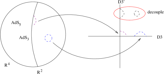
Figure 2: AdS/CFT duality for an Impurity CFT. The duality acts twice. Once for the IIB supergravity on $AdS_{5}\times S^{5}$, and once for DBI theory on $AdS_{3}\times S^{1}$.

2.2 Isometries

In the absence of the probe D3-branes, the isometry group of the $AdS_{5}\times S^{5}$ background is $SO(2,4)\times SO(6)$. The $SO(2,4)$ component acts as conformal transformations on the boundary of $AdS_{5}$, while the $SO(6)\sim SU(4)$ isometry of $S^{5}$ is the R-symmetry of four-dimensional ${\mathcal{N}=4}$ super Yang-Mills theory, under which the six real scalars $X^{4,5,6,7,8,9}$ transform in the vector representation.

In the presence of the probe D3-brane, the $AdS_{5}\times S^{5}$ isometries are broken to the subgroup which leaves the embedding equations of the probe invariant:

$$\!\!\!SO(2,4)\times SU(4)\rightarrow SL(2,R)\times SL(2,R)\times U(1)\times SU(2)_{L}\times SU(2)_{R}\times U(1)$$ (2.7)

Out of the $SO(2,4)$ isometry of $AdS_{5}$ only $SO(2,2)\times U(1)\simeq SL(2,R)\times SL(2,R)\times U(1)$ is preserved. The $SO(2,2)\simeq SL(2,R)\times SL(2,R)$ factor is the isometry group of $AdS_{3}$, while the $U(1)$ factor acts as a phase rotation of the complex coordinates $w=X^{2}+iX^{3}$. Out of the $SO(6)\simeq SU(4)$ isometry of $S^{5}$, only $SO(4)\times U(1)\simeq SU(2)_{L}\times SU(2)_{R}\times U(1)$ is preserved. The $U(1)$ factor here acts as phase rotation of the complex coordinate $y=X^{4}+iX^{5}$, which rotates the $S^{1}$ of the probe worldvolume. The $SO(4)$ component acts on the coordinates $X^{6,7,8,9}$. As we shall see in section 2.3, only a certain combination of the two $U(1)$ factors in (2.7) enters the superconformal algebra. The even part of the superconformal group is $SL(2,R)\times SL(2,R)\times SU(2)_{L}\times SU(2)_{R}\times U(1)$.

2.3 The superconformal algebra

The D3-D3 intersection has a $(4,4)$ superconformal group whose even part is $SL(2,R)\times SL(2,R)\times SU(2)_{L}\times SU(2)_{R}\times U(1)$. We emphasize that this system does not give a standard $(4,4)$ superconformal algebra. Because of the couplings between two and four-dimensional fields, the algebra does not factorize into left and right moving parts. Neither an infinite Virasoro algebra nor an affine Kac-Moody algebra are realized in any obvious way. The superconformal algebra for the D3-D3 system should be thought of as a common “intersection” of two ${\cal N}=4,d=4$ superconformal algebras, both of which are finite. If there is a hidden affine algebra, it should arise via some dynamics which gives a decoupled two-dimensional sector, for which we presently have no evidence.

For comparative purposes, it is helpful to first review the situation for more familiar two-dimensional $(4,4)$ theories with vector multiplets and hypermultiplets, such as those considered in [28]. These theories may have classical Higgs and Coulomb branches which meet at a singularity of the moduli space. For finite coupling, quantum states spread out over both the Higgs and Coulomb branches. However in the infrared (or strong coupling) limit, one obtains a separate $(4,4)$ CFT on the Higgs and Coulomb branches [28]. One argument for the decoupling of the Higgs and Coulomb branches is that the $(4,4)$ superconformal algebra contains an $SU(2)_{l}\times SU(2)_{r}$ R-symmetry with a different origin in the original $SU(2)_{L}\times SU(2)_{R}\times SU(2)$ R-symmetry depending on whether one is on the Higgs branch or Coulomb branch. The CFT scalars must be uncharged under the R-symmetries. This means for example that the original $SU(2)_{L}\times SU(2)_{R}$ factor may be the R-symmetry of the CFT on the Higgs branch but not the Coulomb branch.

For the linear sigma model describing the D3-D3 intersection, a $(4,4)$ super-conformal theory arises only on the Higgs branch, which is parameterized by the two-dimensional scalars of the defect hypermultiplet. On the Coulomb branch, the orthogonal D3-branes are separated by amounts characterized by the VEV’s of four-dimensional scalar fields. One obtains a CFT on the Higgs branch without flowing to the IR, since the gauge fields propagate in four dimensions and the gauge coupling is exactly marginal. Furthermore scalar degrees of freedom of the CFT may carry R-charges, since the R-currents do not break up into purely left and right moving parts. Of course the scalars of the defect hypermultiplet must still be uncharged under the R-symmetries, since for $g_{YM}=0$ the free $(4,4)$ hypermultiplet realizes a conventional two-dimensional $(4,4)$ CFT. However the four-dimensional scalar fields, which are not decoupled at finite $g_{YM}$, transform non-trivially under the R-symmetries of the defect CFT.

In more familiar considerations of the $AdS_{3}/CFT_{2}$ duality, the full Virasoro algebra is realized in terms of diffeomorphisms that leave the form of the metric invariant asymptotically, near the boundary of $AdS_{3}$ [25]. Of these diffeomorphisms, the finite $SL(2,R)\times SL(2,R)$ subalgebra is realized as an exact isometry. However the three-dimensional diffeomorphisms which are asymptotic isometries of $AdS_{3}$, and correspond to higher-order Virasoro generators, do not have an extension into the bulk which leave the $AdS_{5}$ metric asymptotically invariant. The existence of a Virasoro algebra seems to require localized gravity on $AdS_{3}$. This could only be seen through a consideration of the back-reaction. In the defect CFT, the two-dimensional conformal algebra contains only those generators which can be extended to conformal transformations of the four-dimensional parts of the world volume, namely $L_{-1},L_{0},L_{1},\tilde{L}_{-1},\tilde{L}_{0}$ and $\tilde{L}_{1}$.

The ‘global’ $(4,4)$ superconformal algebra of defect CFT gives relations between the dimensions and R-charges of BPS operators. We will later find that these relations are consistent with the spectrum of fluctuations in the probe-$AdS$ background. To construct the relevant part of the algebra, it is helpful to note that the algebra should be a subgroup of an ${\cal N}=4,d=4$ superconformal algebra (or actually an unbroken intersection of two such algebras).

Let us start by writing down the relevant part of the ${\cal N}=4,d=4$ superconformal algebra for the D3-branes in the $0123$ directions. The supersymmetry generators are $Q_{\alpha}^{a}$, where $\alpha=1,2$ is a spinor index and $a=1,\cdots,4$ is an index in the representation ${\bf 4}$ of the $SU(4)$ R-symmetry. The special superconformal generators are $S_{\beta b}$ which are in the ${\bf 4}^{*}$ representation of $SU(4)$. The relevant part of the ${\cal N}=4,d=4$ algebra is then

$$\{Q^{a}_{\alpha},S_{\beta b}\}=\epsilon_{\alpha\beta}({\delta_{b}}^{a}D+4J^{A}(T_{A})^{a}_{b})+\frac{1}{2}{\delta_{b}}^{a}L_{\mu\nu}\sigma^{\mu\nu}_{\alpha\beta}\,,$$ (2.8)

where $D$ is the dilation operator, $J^{A}$ are the operators generating $SU(4)$, and $L_{\mu\nu}$ are the generators of four-dimensional Lorentz transformations. The matrices $(T_{A})^{a}_{b}$ generate the fundamental representation of $SU(4)$, and are normalized such that ${\rm Tr}(T^{A}T^{B})=\frac{1}{2}\delta^{AB}$.

A $(4,4)$ supersymmetry sub-algebra is generated by the supercharges $Q^{a}_{1}\equiv Q^{a}_{+}$ with $a=1,2$, and $Q^{a}_{2}\equiv Q^{a}_{-}$ with $a=3,4$, on which an $SU(2)_{L}\times SU(2)_{R}\times U(1)$ subgroup of the orginal $SU(4)$ R-symmetry acts. The embedding of the $SU(2)_{L}\times SU(2)_{R}\times U(1)$ generators in $SU(4)$ is as follows:

$$SU(2)_{L}:\begin{pmatrix}\frac{1}{2}\sigma^{A}&0\cr 0&0\end{pmatrix},\quad SU(2)_{R}:\begin{pmatrix}0&0\cr 0&\frac{1}{2}\sigma^{B}\end{pmatrix},\quad U(1):\frac{1}{\sqrt{8}}\begin{pmatrix}-I&0\cr 0&I\end{pmatrix}\,.$$ (2.9)

The unbroken $SU(2)_{L}\times SU(2)_{R}$ R-symmetry corresponds to rotations in the directions $6,7,8,9$ transverse to both stacks of D3-branes, while the unbroken $U(1)$ describes rotation in the $45$ plane. These symmetries act on adjoint scalars. Since the R-currents of the CFT do not break up into left and right moving parts, there is no requirement that four-dimensional scalars are uncharged under R-symmetries. We shall call the generator of rotations in the $45$ plane $J_{45}$, and normalize it such that the supercharges $Q^{a}_{\pm}$ have $J_{45}$ eigenvalue $\pm 1/2$. The special superconformal generators of the $(4,4)$ sub-algebra are $S_{b2}\equiv S_{b-}$ with $b=1,2$ and $S_{b1}\equiv S_{b+}$ with $b=3,4$. The term in the $(4,4)$ algebra inherited from (2.8) is then

$$\{Q^{a}_{+},S_{b-}\} ={\delta_{b}}^{a}D+2J^{L}_{A}(\sigma^{A})^{a}_{b}+\delta^{a}_{b}J_{45}+\delta^{a}_{b}L_{01}+\delta^{a}_{b}L_{23}\,,$$ (2.10)

$$\{Q^{a}_{-},S_{b+}\} =-\delta_{b}^{a}D-2J^{R}_{A}(\sigma^{A})^{a}_{b}+\delta^{a}_{b}J_{45}+\delta^{a}_{b}L_{01}+\delta^{a}_{b}L_{23}\,.$$ (2.11)

The unbroken Lorentz generators are $L_{01}$ and $L_{23}$. Note that from a two-dimensional point of view, the Lorentz transformations are generated by $L_{01}$, whereas $L_{23}$ is an R-symmetry.

For the orthogonal D3-branes spanning $0,1,4,5$, rotations in the $45$ plane are Lorentz generators $L_{45}$ rather than a subgroup of $SU(4)$. The rotations in the $23$ plane are an unbroken $U(1)$ part of the $SU(4)$ R-symmetry rather than a Lorentz transformation. This distinction is illustrated in figure 3.

Figure 3: Decomposition of the two $SU(4)$ R-symmetries.

From the two-dimensional point of view, both $23$ and $45$ rotations are $U(1)$ R-symmetries. If we write $L_{23}=J_{23},\,L_{45}=J_{45}$ and define ${\cal J}=J_{23}+J_{45}$, then the terms (2.10) and (2.11) become

$$\{Q^{a}_{+},S_{b-}\} ={\delta_{b}}^{a}(L_{01}+D)+2J^{L}_{A}(\sigma^{A})^{a}_{b}+\delta^{a}_{b}{\cal J}\,,$$ (2.12)

$$\{Q^{a}_{-},S_{b+}\} =\delta_{b}^{a}(L_{01}-D)-2J^{R}_{A}(\sigma^{A})^{a}_{b}+\delta^{a}_{b}{\cal J}\,.$$ (2.13)

which are applicable to both stacks of D3-branes. This forms part of the $(4,4)$ superconformal algebra of the full D3-D3 system. The charge ${\cal J}$ plays a somewhat unusual role. From the point of view of the bulk four-dimensional fields, ${\cal J}$ is a combination of an R-symmetry and a Lorentz symmetry, under which the preserved supercharges are invariant. As we will see later, the fields localized at the two-dimensional intersection are not charged under ${\cal J}$. Upon decoupling the four-dimensional fields by taking $g=0$, the two-dimensional sector becomes a free $(4,4)$ superconformal theory with an affine $SU(2)_{L}\times SU(2)_{R}$ R-symmetry. However, for $g_{YM}\neq 0$, the algebra does not factorize into left and right moving parts.

The algebra (2.12, 2.13) determines the dimensions of the BPS superconformal primary operators, which are annihilated by all the $S$’s and some of the $Q$’s. The bounds on dimensions due to the superconformal algebra are best obtained in Euclidean space. The Euclidean $(4,4)$ algebra of the defect CFT contains the terms

$$\{{\cal Q}^{a}_{1/2},{\cal Q}_{1/2}^{b\dagger}\}=2\delta^{a}_{b}L_{0}+2J^{L}_{A}({\sigma^{A}})^{a}_{b}+\delta^{a}_{b}{\cal J}\,,$$ (2.14)

$$\{\tilde{\cal Q}^{a}_{1/2},\tilde{\cal Q}_{1/2}^{b\dagger}\}=2\delta^{a}_{b}\tilde{L}_{0}+2J^{R}_{A}({\sigma^{A}})^{a}_{b}-\delta^{a}_{b}{\cal J}\,.$$ (2.15)

For $a=b$, the left hand side of (2.14) and (2.15) are positive operators, leading to the bounds

$$h+j^{L}_{3}+\textstyle\frac{1}{2}{\cal J}\geq 0\,,$$ (2.16)

$$h-j^{L}_{3}+\textstyle\frac{1}{2}{\cal J}\geq 0\,,$$ (2.17)

$$\tilde{h}+j^{R}_{3}-\textstyle\frac{1}{2}{\cal J}\geq 0\,,$$ (2.18)

$$\tilde{h}-j^{R}_{3}-\textstyle\frac{1}{2}{\cal J}\geq 0\,,$$ (2.19)

some of which are saturated by the BPS super-conformal primaries. As always, the dimensions are $\Delta=h+\tilde{h}$, with $h=\tilde{h}$ for scalar operators.

3 Fluctuations in the probe-supergravity background

Following the conjecture put forth in [7] and elaborated upon in [8], we expect the holographic duals of defect operators localized on the intersection are open strings on the probe D$3^{\prime}$, whose world volume is an $AdS_{3}\times S^{1}$ submanifold of $AdS_{5}\times S^{5}$. The operators with protected conformal dimensions should be dual to probe Kaluza-Klein excitations at “sub-stringy” energies, $m^{2}\ll\lambda/L^{2}$. In this section we shall find the mass spectra of these excitations. Later we will find this spectrum to be consistent with the dimensions of operators localized on the intersection.

3.1 The probe-supergravity system

The full action describing physics of the background as well as the probe is given by

$$S_{bulk}=S_{IIB}+S_{DBI}+S_{WZ}\,.$$ (3.1)

The contribution of the bulk supergravity piece of the action in Einstein frame is

$$S_{IIB}=\frac{1}{2\kappa^{2}}\int d^{10}x\sqrt{-g}\left(R-\frac{1}{2}e^{2\Phi}(\partial\Phi)^{2}+\cdots\right)$$ (3.2)

where $2\kappa^{2}=(2\pi)^{7}g_{s}^{2}l_{s}^{8}$. The dynamics of the probe D3-brane is given by a Dirac-Born-Infeld term and a Wess-Zumino term [29],

$$S_{DBI}+S_{WZ}=-T_{D3}\int d^{4}\sigma e^{-\Phi}\sqrt{-\det\left(g_{ab}^{PB}+e^{-\Phi/2}{\cal F}_{ab}\right)}\,+\,T_{D3}\int C^{(4)}_{PB}\,.$$ (3.3)

The metric $g_{ab}^{PB}$ is the pull back of the bulk $AdS_{5}\times S^{5}$ metric to the world volume of the probe, while $C^{(4)}_{PB}$ is the pull back of the bulk Ramond-Ramond four form.

We work in a static gauge where the world volume coordinates of the brane are identified with the space time coordinates by $\sigma^{a}\sim x^{0},x^{1},u,\xi$. With this identification the DBI action is

$$S_{DBI}=-T_{D3}\int d^{4}\sigma\sqrt{-\det\left(g_{ab}+\partial_{a}Z^{i}\partial_{b}Z^{j}g_{ij}+e^{-\Phi/2}{\cal F}_{ab}+2g_{ai}\partial_{b}Z^{i}\right)}$$ (3.4)

where $i,j$ label the transverse directions to the probe and the scalars $Z^{i}$ represent the fluctuations of the transverse scalars $X^{2},X^{3},\theta,\phi,\rho,\varphi$. Also, ${\cal F}_{ab}=B_{ab}+2\pi l_{s}^{2}F_{ab}$ is the total world volume field strength. Henceforth we will only consider the open string fluctuations on the probe and thus drop terms involving closed string fields$B_{ab}$ and $g_{ai}$. To quadratic order in fluctuations, the action takes the form

$$S_{DBI} =-T_{D3}L^{4}\int d^{4}\sigma\sqrt{\bar{g}_{4}}(1-\frac{1}{2}\phi^{2}-\frac{1}{2}\theta^{2}-\frac{1}{2}\rho^{2}-\frac{1}{2}\varphi^{2}+\frac{1}{2}\partial_{a}\theta\partial^{a}\theta+\frac{1}{2}\partial_{a}\phi\partial^{a}\phi$$

$$+\frac{1}{2}\partial_{a}\rho\partial^{a}\rho+\frac{1}{2}\partial_{a}\varphi\partial^{a}\varphi+\frac{1}{2u^{2}}\partial_{a}X^{2}\partial^{a}X^{2}+\frac{1}{2u^{2}}\partial_{a}X^{3}\partial^{a}X^{3}+\frac{1}{4}(2\pi l_{s}^{2})^{2}F_{ab}F^{ab})$$ (3.5)

where $\bar{g}_{4}$ is the determinant of the rescaled $AdS_{3}\times S^{1}$ metric $\bar{g}^{4}_{ab}$ given by

$$d\bar{s}^{2}=\frac{1}{u^{2}}(-dt^{2}+dx^{2}_{1}+du^{2})+d\xi^{2}.$$ (3.6)

To obtain the Wess-Zumino term $S_{WZ}$ we require the pull back of the bulk RR-four form to the probe:

$$C^{PB}_{abcd} = C_{abcd}+4\partial_{[a}Z^{i}C_{bcd]i}+6\partial_{[a}Z^{i}\partial_{b}Z^{j}C_{cd]ij}$$ (3.7)

$$+ 4\partial_{[a}Z^{i}\partial_{b}Z^{j}\partial_{c}Z^{k}C_{d]ijk}+\partial_{[a}Z^{i}\partial_{b}Z^{j}\partial_{c}Z^{k}\partial_{d]}Z^{l}C_{ijkl}\,.$$

In the $AdS_{5}\times S^{5}$ background, one can choose a gauge in which

$$C^{(4)}_{0123}=\frac{L^{4}}{u^{4}}$$ (3.8)

while the remaining components, which are determined by the self duality of $dC^{(4)}$, contribute only to terms in the pull back with more than two $\partial Z$’s. We do not need such terms to obtain the fluctuation spectrum. The quadratic term arising from (3.8) is

$$C_{PB}^{(4)}=\left(\partial_{u}X^{2}\partial_{\xi}X^{3}-\partial_{u}X^{3}\partial_{\xi}X^{2}\right)C_{0123}dt\wedge dx^{1}\wedge du\wedge d\xi\,.$$ (3.9)

The Wess-Zumino action is then

$$S_{WZ}=T_{D3}L^{4}\int d^{4}\sigma\frac{1}{u^{4}}(\partial_{u}X^{2}\partial_{\xi}X^{3}-\partial_{u}X^{3}\partial_{\xi}X^{2})\,.$$ (3.10)

3.2 $S^{1}$ fluctuations inside $S^{5}$

From eqn. (3.5) one can see that the angular fluctuations $\theta,\phi,\rho$ and $\varphi$ are minimally coupled scalars on $AdS_{3}\times S^{1}$. Interestingly they have $m^{2}=-1$ which, although negative, satisfies (saturates) the Breitenlohner-Freedman bound $m^{2}\geq-d^{2}/4$, where $d=2$ for $AdS_{3}$. Expanding in Fourier modes on $S^{1}$, i.e., $\theta=\theta_{l}e^{il\xi}$ the Kaluza-Klein modes of these scalars have $m^{2}=-1+l^{2}$. This leads to a spectrum of conformal dimensions of dual defect operators given by $\Delta_{\pm}=\frac{d}{2}\pm\sqrt{\frac{d^{2}}{4}+m^{2}}=1\pm l$, where $d=2$. For $l>0$ one should choose the positive branch for unitarity, while for $l<0$ one should choose the negative branch. To leading order in fluctuations of the $S^{1}$ embedding we see that

$$x^{6} =-r\varphi$$

$$x^{7} =-r\rho$$

$$x^{8} =-r\theta$$

$$x^{9} =-r\phi\,.$$ (3.11)

Thus the angular variables $\phi,\theta,\rho$ and $\varphi$ belong to a $(\frac{1}{2},\frac{1}{2})$ multiplet of $SU(2)_{L}\times SU(2)_{R}$. Moreover, these fluctuations have $J_{23}=0$ and $J_{45}=l$ such that the $U(1)$ charge appearing in the algebra (2.14, 2.15) is ${\cal J}=l$. Each fluctuation in the series $\Delta=l+1$ saturates one of the bounds in (2.16)-(2.19), so these fluctuations should be dual to $1/4$ BPS operators.

3.3 $AdS_{3}$ fluctuations inside $AdS_{5}$

Let us now compute the conformal dimensions of the operators dual to the scalars which describe the fluctuations of the probe inside of $AdS_{5}$. From eqns. (3.5) and (3.10) the action for $X^{2}$ and $X^{3}$ is

$$S_{2,3} = -T_{D3}L^{4}\int d^{4}\sigma\sqrt{\bar{g}_{4}}\left(\frac{1}{2u^{2}}\partial_{a}X^{2}\partial^{a}X^{2}+\frac{1}{2u^{2}}\partial_{a}X^{3}\partial^{a}X^{3}\right)$$ (3.12)

$$+ T_{D3}L^{4}\int d^{4}\sigma\left(\frac{1}{u^{4}}\partial_{\xi}X^{2}\partial_{u}X^{3}-\frac{1}{u^{4}}\partial_{u}X^{2}\partial_{\xi}X^{3}\right)\,.$$

Writing $\sqrt{2\pi}X^{i}=X^{i}_{l}\exp(il\xi)$ for $i=2,3$ and doing the integral over $\xi$ gives

$$S_{2,3} = -T_{D3}L^{4}\int d^{3}\sigma\sqrt{g_{3}}\left(1+\frac{1}{2u^{2}}(g_{3}^{ab}\partial_{a}X_{-l}^{i}\partial_{b}X^{i}_{l}+l^{2}X^{i}_{-l}X^{i}_{l})\right)$$ (3.13)

$$+ T_{D3}L^{4}\int d^{3}\sigma\frac{1}{u^{4}}\left(ilX_{l}^{3}\partial_{u}X_{-l}^{2}-ilX^{2}_{l}\partial_{u}X_{-l}^{3}\right).$$

where $g^{3}_{ab}$ is the metric for the $AdS_{3}$ geometry

$$ds^{2}=\frac{1}{u^{2}}\left(-dt^{2}+dx_{1}^{2}+du^{2}\right)\,.$$ (3.14)

The $X^{2},X^{3}$ mixing in the Wess-Zumino term is diagonalized by working with the field $w_{l}\equiv X^{2}_{l}+iX^{3}_{l}$, in terms of which the action is

$$S_{w}=-T_{D3}L^{4}\int d^{3}\sigma\sqrt{g_{3}}\frac{1}{2u^{2}}(g^{ab}_{3}\partial_{a}w_{l}^{*}\partial_{b}w_{l}+l^{2}w^{*}_{l}w_{l})$$

$$+T_{D3}L^{4}\int d^{3}\sigma\frac{1}{2u^{4}}\partial_{u}(lw^{*}_{l}w_{l})\,.$$ (3.15)

The usual action for a scalar field in $AdS_{3}$ is obtained by defining $\tilde{w}_{l}=w_{l}/u$, giving

$$S_{w}=-T_{D3}L^{4}\int d^{3}\sigma\sqrt{g_{3}}\frac{1}{2}\left(g_{3}^{ab}\partial_{a}\tilde{w}^{*}_{l}\partial_{b}\tilde{w}_{l}+(l^{2}-4l+3)\tilde{w}^{*}_{l}\tilde{w}_{l}\right)$$ (3.16)

$$+T_{D3}L^{4}(l-1)\int d^{3}\sigma\frac{1}{2}\partial_{u}(\frac{1}{u^{2}}\tilde{w}^{*}_{l}\tilde{w}_{l})\,.$$ (3.17)

The surface term (3.17) does not effect the equations of motion, but will be significant later when we compute correlation functions of the dual operators. Inserting the spectrum $m^{2}=l^{2}-4l+3$ into the standard formula $\Delta=d/2\pm\sqrt{d^{2}/4+m^{2}}$ gives

$$\Delta=1\pm|l-2|\,.$$ (3.18)

This gives two series of dimensions, $\Delta=l-1$ and $\Delta=3-l$, which are possible in the ranges of $l$ for which $\Delta$ is non-negative. The entry in the AdS/CFT dictionary for the series $\Delta=l-1$ holds several remarkable surprises which we will encounter later.

3.4 Gauge field fluctuations

We finally turn to the fluctuations of the world volume gauge field. It is convenient to rescale fields according to $\hat{F}_{ab}=2\pi l_{s}^{2}F_{ab}$ so that the gauge field fluctuations have the same normalization as the scalars in the previous subsection. We have

$$S_{gauge} = -T_{D3}L^{4}\int d^{4}\sigma\sqrt{\bar{g}_{4}}\frac{1}{4}\hat{F}_{ab}\hat{F}^{ab}\,.$$ (3.19)

$$= -T_{D3}L^{4}\int d^{4}\sigma\sqrt{\bar{g}_{4}}\frac{1}{4}\left(\hat{F}_{\alpha\beta}\hat{F}^{\alpha\beta}+2\hat{F}_{\xi\alpha}\hat{F}^{\xi\alpha}\right)\,.$$

In order to decouple the $AdS_{3}$ components of the gauge field from that on the $S^{1}$ it is convenient to work in the gauge $A_{\xi}=0$. Expanding the rest of the components in Fourier modes on the $S^{1}$ so that $A_{\alpha}=\hat{A}_{\alpha}e^{il\xi}$ the action becomes

$$S_{gauge}=-T_{D3}L^{4}\int d^{3}\sigma\sqrt{\bar{g}_{3}}\frac{1}{4}\left(\hat{F}_{\alpha\beta}\hat{F}^{\alpha\beta}+2l^{2}\hat{A}_{\alpha}\hat{A}^{\alpha}\right)\,.$$ (3.20)

The equations of motion are easily found to be

$$D^{\alpha}\hat{F}_{\alpha\beta}+l^{2}\hat{A}_{\beta}=0$$ (3.21)

which are just the Maxwell-Proca equations for a vector field with $M^{2}=l^{2}$. Using the standard relation $\Delta=d/2\pm\sqrt{(d-2)^{2}/4+M^{2}}$ relating the mass of a vector field to the dimension of its dual operator we find the spectrum

$$\Delta_{\pm}=1\pm l$$ (3.22)

which for $l>1$ requires us to choose the positive branch.

4 Correlators from strings on the probe-supergravity background

The rules for using classical supergravity in an AdS background to compute CFT correlators have a natural generalization to defect CFT’s dual to AdS probe-supergravity backgrounds. The generating function for correlators in the defect CFT is identified with the classical action of the combined probe-supergravity system with boundary conditions set by the sources. This approach was used to compute correlators in the dCFT describing the D3-D5 system in [8]. Without worrying yet about what the dual operators are, we will do the same for the D3-D3 system here. In this section we will highlight some peculiar features of this defect CFT. First it will be shown that the correlators of operators dual to probe fluctuations are independent of the ’t Hooft coupling, at least in the limit that the ’t Hooft coupling is large. Second, the two-point function of operators dual to one set of fluctuations discussed in section (3.3) will be shown to vanish. Correlators involving both defect and bulk fields are presented in appendix A.

4.1 Independence of the correlators on the ’t Hooft coupling

As in refs. [30, 31, 8] it is useful to work with a Weyl rescaled metric

$$g_{MN}=L^{2}\bar{g}_{MN}$$ (4.1)

where $L^{2}=\sqrt{g_{s}N}l_{s}^{2}$. In terms of the rescaled metric, the supergravity action (3.2) becomes

$$\frac{L^{8}}{2\kappa^{2}}\int d^{10}x\sqrt{-\bar{g}}\left(R-\frac{1}{2}e^{2\Phi}(\partial\Phi)^{2}+\cdots\right)\sim N^{2}\int d^{10}x\sqrt{-\bar{g}}\left(R-\frac{1}{2}e^{2\Phi}(\partial\Phi)^{2}+\cdots\right)$$ (4.2)

As in the usual AdS/CFT correspondence correlation functions of gauge invariant operators in the bulk of $\mathcal{N}=4$ SYM at large ’t Hooft coupling are calculated by expanding this action around the $AdS_{5}\times S^{5}$ vacuum of type IIB. Here the presence of the probe D3-brane will make additional contributions both through its world volume fields but also through the pull backs of the $AdS_{5}\times S^{5}$ fields. Terms involving the pull backs are dual to couplings between the bulk of the field theory and the codimension 2 defect. After Weyl rescaling the metric as above, the D3-brane probe action $S_{DBI}+S_{WZ}$ becomes,

$$-L^{4}T_{D3}\int d^{4}{\sigma}\sqrt{\bar{g}}(1+{\rm fluctuations})\sim N\int d^{4}{\sigma}\sqrt{\bar{g}}(1+{\rm fluctuations})\,.$$ (4.3)

Notice that the dependence on the ’t Hooft coupling $\lambda=g_{s}N$ has completely dropped out of the normalization of the action! Generic correlation functions involving $n$ fields $\psi$ living on the D3-brane probe and $m$ fields $\phi$ from the bulk of $AdS_{5}$ arise from

$$S_{DBI} = N\int d^{4}\sigma\left((\partial\psi)^{2}+\phi^{m}\psi^{n}\right)$$ (4.4)

$$= \int d^{4}\sigma\left((\partial\psi^{\prime})^{2}+\frac{1}{N^{n/2+m-1}}\psi^{\prime}{}^{n}\phi^{\prime}{}^{m}\right)$$

where $\psi^{\prime}=N^{1/2}\psi$ and $\phi^{\prime}=N\phi$ are the canonically normalized probe and $AdS_{5}$ fields respectively. The $N$ dependence of correlators which follows from (4.4) is consistent with what one expects in the planar limit. It is interesting that none of these correlation functions has any dependence on $\lambda$, at least for large $\lambda$ where the $AdS$ probe-supergravity description is valid.

4.2 Correlators from probe fluctuations inside AdS₅: a surprise

Let us now compute the correlation functions associated to the fluctuations $w_{l}$ of the probe brane inside $AdS_{5}$. For a classical solution of the equation of motion, the action given by the sum of (3.16) and (3.17) is given by the surface term

$$S_{cl}=-T_{D3}L^{4}\int d^{3}\sigma\frac{1}{2}\partial_{u}\left[\frac{1}{u}\tilde{w}_{l}^{*}\partial_{u}\tilde{w}_{l}-(l-1)\frac{1}{u^{2}}\tilde{w}_{l}^{*}\tilde{w}_{l}\right]\,.$$ (4.5)

The first term in this expression is of the standard form obtained in AdS/CFT, for instance in [32]. The new feature here which does not appear in standard AdS computations is the extra surface term with coefficient $(l-1)$. This term has dramatic consequences. To see this we compute the two-point function of the operator dual to $w_{l}$ following the procedure of [32]. We introduce an $AdS_{3}$ boundary at $u=\epsilon$ and evaluate the action (4.5) for a solution of the form

$$w_{l}(u,\vec{k})=K^{(l)}(u,\vec{k})\,w_{l}{}^{b}(\vec{k})$$ (4.6)

in momentum space satisfying the boundary conditions

$$\lim_{u\rightarrow\epsilon}K^{(l)}(u,\vec{k})=1,\qquad\lim_{u\rightarrow\infty}K^{(l)}(u,\vec{k})=0\,.$$ (4.7)

The solution of the wave equation with these boundary conditions is

$$K^{(l)}(u,\vec{k})=\frac{u}{\epsilon}\frac{{\cal K}_{\nu}(u|\vec{k}|)}{{\cal K}_{\nu}(\epsilon|\vec{k}|)}\,,$$ (4.8)

where $\nu=\Delta-1$ and ${\cal K}_{\nu}(x)$ is the modified Bessel function which vanishes at $x\rightarrow\infty$. Note that this coincides with the calculation of [32] where in this case $d=2$. The two-point function is given by

$$\langle{\cal O}(\vec{k}){\cal O}(\vec{k}^{\prime})\rangle \equiv-\frac{\delta^{2}}{\delta w_{l}{}^{b}(\vec{k})\delta w_{l}{}^{b}(\vec{k}^{\prime})}S_{cl}\Big{|}_{w_{l}{}^{b}=0}$$

$$=-\frac{1}{\epsilon}\delta(\vec{k}+\vec{k}^{\prime})\lim_{u\rightarrow\epsilon}\left[\partial_{u}K(u,\vec{k})-(l-1)\frac{1}{u}K(u,\vec{k})\right]\,,$$ (4.9)

with $S_{cl}$ the Fourier transform of (4.5).

The non-local part of the two-point function is obtained by expanding ${\cal K}_{\nu}$ in a power series for small argument, keeping only the term which scales like $\varepsilon^{2(\Delta-2)}$. The more singular terms give rise to local contact terms of the form $\square^{2}\delta(x-y)$ and are dropped. The non-local contribution to the two-point function is given by

$$\langle{\cal O}(\vec{k}){\cal O}(\vec{k}^{\prime})\rangle =\delta(\vec{k}+\vec{k}^{\prime})\lim_{u\rightarrow\epsilon}\left[-\epsilon^{-1}(\epsilon k)^{-1}\partial_{u}\left(\frac{2^{-2(\Delta-1)}\frac{\Gamma(2-\Delta)}{\Gamma(\Delta)}(ku)^{\Delta}}{(k\epsilon)^{1-\Delta}}\right)\right.$$

$$\left.\qquad\qquad\qquad\qquad\ +\,(l-1)\,\epsilon^{-2}(\epsilon k)^{-1}\frac{2^{-2(\Delta-1)}\frac{\Gamma(2-\Delta)}{\Gamma(\Delta)}(ku)^{\Delta}}{(k\epsilon)^{1-\Delta}}\right]\,.$$ (4.10)

The first of the two terms coincides exactly with the standard AdS calculation of [32], whereas the second term is an additional feature due to the presence of the probe brane. Remarkably, there is an exact cancellation between the first and the second term in (4.10) for the series $\Delta=l-1$. Thus for these fluctuations the usual calculation does not give a power law correlation function of the form $1/x^{2\Delta}$. When we obtain the operators dual to these fluctuations, it will become clear that one should not find a power law. In particular, the lowest mode in this series is the operator which parameterizes the classical Higgs branch.

5 The conformal field theory of the D3-D3
intersection

Thus far we have only studied the dCFT on the D3-D3 intersection in terms of its holographic dual, without ever writing the action. In this section we will construct the action describing $N$ D3-branes orthogonally intersecting $N^{\prime}$ D$3^{\prime}$-branes over two common dimensions. In the notation of [10] this system is known as $(1|\rm D3\bot D3^{\prime})$. In the discussion of holography it was assumed that $N\rightarrow\infty$ with $g_{YM}^{2}N$ and $N^{\prime}$ fixed, such that the open strings with both endpoints on the D3^′-brane decoupled. We will not make this assumption in constructing the action.

The $\mathcal{N}=4$ SYM $SU(N)$ theory located on the D3-branes and the $\mathcal{N}=4$ SYM $SU(N^{\prime})$ theory located on the D$3^{\prime}$-branes couple to a $(4,4)$ hypermultiplet at a two-dimensional impurity. Although $(4,4)$ supersymmetry is preserved, it is convenient to work with $(2,2)$ superspace. The world volume of both stacks of D3-branes can be viewed as two $\mathcal{N}=2,d=4$ superspaces, intersecting over a two-dimensional $(2,2)$ superspace. One of the $\mathcal{N}=2,d=4$ superspaces is spanned by

$${\cal X}\sim(z^{+},z^{-},w,\bar{w},\theta_{i}^{\alpha},\bar{\theta}^{i}_{\dot{\alpha}})\,,$$ (5.1)

with $z^{\pm}=X^{0}\pm X^{1}$ and $w=X^{2}+iX^{3}$. The index $\alpha$ is a spinor index with values $1,2$, while the index $i$ accounts for the $\mathcal{N}=2$ supersymmetry and has values $1,2$. The other $\mathcal{N}=2,d=4$ superspace is spanned by

$${\cal X}^{\prime}\sim(z^{+},z^{-},y,\bar{y},\Theta_{i}^{\alpha},\bar{\Theta}^{i}_{\dot{\alpha}})\,,$$ (5.2)

where $y=X^{4}+iX^{5}$ and one makes the identification

$$\theta^{1}_{(1)}=\Theta^{1}_{(1)}\equiv\theta^{+}\,,$$ (5.3)

$$\theta^{2}_{(2)}=\Theta^{2}_{(2)}\equiv\bar{\theta}^{-}\,.$$ (5.4)

This is not the unique choice. For instance one could have written $\theta^{2}_{(2)}=\Theta^{2}_{(2)}\equiv\theta^{-}$ which is related to the first choice by mirror symmetry [33]. The intersection is the $(2,2),d=2$ superspace spanned by

$${\cal X}\cap{\cal X}^{\prime}\sim(z^{+},z^{-},\theta^{+},\theta^{-},\bar{\theta}^{+},\bar{\theta}^{-})\,.$$ (5.5)

All the degrees of freedom describing the D3-D3^′ intersection can be written in $(2,2)$ superspace. For instance the D3-D3 strings, which are not restricted to the intersection, can be described by $(2,2)$ superfields carrying extra (continuous) labels $w,\bar{w}$. Similiarly superfields associated to the D$3^{\prime}$-D$3^{\prime}$ strings carry the extra labels $y,\bar{y}$. Fields associated to D3-D$3^{\prime}$ strings are localized on the intersection and have no extra continuous labels.

Due to the breaking of four-dimensional supersymmetry by the couplings to the degrees of freedom localized at the intersection, it is convenient to write the action in a language in which the unbroken $(2,2)$ symmetry is manifest. This leads to a somewhat unusual form for the four-dimensional parts of the action. One way to obtain this action is somewhat akin to deconstruction [34]. The basic idea is to start with a conventional $(4,4)$ two-dimensional action in $(2,2)$ superspace, add an extra continuous label $w,\bar{w}$ to all the fields, and then try to add terms preserving $(4,4)$ supersymmetry such that there is a (non-manifest) four-dimensional Lorentz invariance. A four-dimensional Lorentz invariant theory which has a two-dimensional $(4,4)$ supersymmetry must also have ${\cal N}=4$ supersymmetry in four dimensions. The procedure of constructing a supersymmetric D-dimensional theory using a lower dimensional superspace has been employed in several contexts [35, 9, 36]. The reader wishing to skip directly to the action of the D3-D3 intersection in $(2,2)$ superspace may proceed to section 5.2.

5.1 Four-dimensional actions in lower dimensional superspaces

The approach of building four-dimensional Lorentz invariance starting with a conventional $(4,4)$ supersymmetric theory is an indirect but effective way to obtain the ${\cal N}=4,d=4$ super Yang-Mills action in a two-dimensional superspace. There is also a more direct approach which gives a $(2,2)$ superspace representation for the part of the ${\cal N}=4,d=4$ action containing only the ${\cal N}=2,d=4$ vector multiplet. The ${\cal N}=2,d=4$ vector multiplet has a straightforward decomposition under two-dimensional $(2,2)$ supersymmetry. On the other hand, there is no off-shell ${\cal N}=2,d=4$ formalism for the hypermultiplet, unless one uses harmonic superspace. We demonstrate the decomposition of the vector multiplet below. This provides a useful check of at least part of the action appearing in section 5.2.

5.1.1 Embedding $(2,2)$, $d=2$ in $\mathcal{N}=2$, $d=4$

We begin by showing how to embed $(2,2)$, $d=2$ superspace into $\mathcal{N}=2$, $d=4$ superspace. The $\mathcal{N}=2,d=4$ superspace is parametrized by ($z^{+},z^{-},w,\bar{w}$, $\theta_{(i)}^{\alpha}$, $\bar{\theta}^{(i)}_{\dot{\alpha}}$). For the embedding let us redefine these coordinates as

$$\theta^{+} \equiv\theta_{(1)}^{1},\quad\theta\!\!\!/^{+}\equiv\theta_{(2)}^{1}\,,$$

$$\bar{\theta}^{-} \equiv\theta_{(2)}^{2},\quad\theta\!\!\!/^{-}\equiv\theta_{(1)}^{2}\,.$$ (5.6)

In the absence of central charges, the $\mathcal{N}=2$, $d=4$ supersymmetry algebra is

$$\{Q_{(i)\alpha},\bar{Q}^{(j)}{}_{\dot{\beta}}\} =2\rho^{\mu}_{\alpha\dot{\beta}}P_{\mu}\delta_{i}^{j},\qquad i,j=1,2\,,$$

$$\{Q_{(i)\alpha},Q_{(j)\beta}\} =\{\bar{Q}^{(i)}{}_{\dot{\alpha}},\bar{Q}^{(j)}{}_{\dot{\beta}}\}=0\,$$ (5.7)

with Pauli matrices $\rho^{\mu}$ given by Eq. (B.2). We define supersymmetry charges $Q_{+}\equiv Q_{(1)1}$, $\bar{Q}_{-}\equiv Q_{(2)2}$, $Q\!\!\!\!/\,_{+}\equiv Q_{(2)1}$, and ${{Q\!\!\!\!/\,_{-}}\equiv Q_{(1)2}}$. Following the methods of refs. [37, 38], we introduce a superspace defect at

$$w=0,\quad\theta\!\!\!/^{+}=\theta\!\!\!/^{-}=0\,,$$

which implies that the generators $P_{2}$, $P_{3}$, $Q\!\!\!\!/\,_{\pm}$, and $\bar{Q}\!\!\!\!/\,_{\pm}$ are broken. The unbroken subalgebra of (5.7) is generated by $Q_{\pm}$ and $\bar{Q}_{\pm}$ and turns out to be the $(2,2)$, $d=2$ supersymmetry algebra given by

$$\{Q_{\pm},\bar{Q}_{\pm}\}=2(P_{0}\pm P_{1})\,.$$ (5.8)

Other anticommutators of the $Q$’s vanish due to the absence of central charges.

5.1.2 $\mathcal{N}=2$, $d=4$ Super Yang-Mills action in $(2,2)$, $d=2$ language

In order to derive the $\mathcal{N}=2$ Yang-Mills action in $(2,2)$ language, we decompose the four-dimensional $\mathcal{N}=2$ abelian vector superfield $\Psi$ in terms of a two-dimensional $(2,2)$ chiral superfield $\Phi$, a twisted chiral superfield $\Sigma$, and a vector superfield $V$. In the abelian case, the twisted chiral superfield (see e.g. Ref. [33, 39]) is related to the vector multiplet by

$$\Sigma\equiv\bar{D}_{+}D_{-}V$$ (5.9)

and satisfies $\bar{D}_{+}\Sigma=D_{-}\Sigma=0$. The $(2,2)$ vector and chiral superfields can be obtained by dimensional reduction of their ${\cal N}=1,d=4$ counterparts.

In appendix C we show that the $\mathcal{N}=2$, $d=4$ vector supermultiplet $\Psi$ decomposes into

$$\Psi=-i\Sigma+\theta\!\!\!/^{+}\bar{D}_{+}\left(\bar{\Phi}-\partial_{\bar{w}}V\right)+\theta\!\!\!/^{-}D_{-}\left(\Phi-\partial_{w}V\right)+\theta\!\!\!/^{+}\theta\!\!\!/^{-}G\,$$ (5.10)

where $\partial_{w}$ is the transverse derivative and $G$ an auxiliary $(2,2)$ superfield. An interesting result of the decomposition is that the auxiliary field $D$ of the twisted chiral superfield $\Sigma$ is related to the component $D^{\prime}$ and transverse derivatives of the components $v^{\prime}_{2}$ and $v^{\prime}_{3}$ of the four-dimensional vector superfield,

$$D=\frac{1}{\sqrt{2}}\left(D^{\prime}+f^{\prime}_{32}\right)\,,$$ (5.11)

where $f^{\prime}_{32}=\partial_{3}v^{\prime}_{2}-\partial_{2}v^{\prime}_{3}$. Note that in distinction to the conformal field theory dual to the $(2|\rm D3\perp D5)$ intersection studied in [8, 9] there are no transverse derivatives like $\partial_{w}\phi^{\prime}$ in the auxiliary fields $F$ of the (2,2) superfield $\Phi$.

With the above decomposition of $\Psi$, we can now write down the $\mathcal{N}=2$, $d=4$ (abelian) Yang-Mills action in (2,2) language. Substituting Eq. (5.10) with $G=\bar{D}_{+}D_{-}(i\Sigma^{\dagger}+...)$ into the usual form of the YM action, we find

$$\frac{1}{4\pi}{\rm\,Im\,}\tau\int d^{4}xd^{2}\theta_{(1)}d^{2}\theta_{(2)}\,\frac{1}{2}\Psi^{2}$$ (5.12)

$$=\frac{1}{4\pi}{\rm\,Im\,}\tau\int d^{4}xd^{4}\theta\,\left(\bar{\Sigma}\Sigma+\bar{\Phi}\Phi+\partial_{\bar{w}}V\Phi-\bar{\Phi}\partial_{w}V-\partial_{\bar{w}}V\partial_{w}V\right),$$

with $d^{4}\theta=\frac{1}{4}d\theta^{+}d\theta^{-}d\bar{\theta}^{+}d\bar{\theta}^{-}$. From this one can easily deduce the corresponding non-abelian Yang-Mills action for vanishing $\theta$ angle,

$$S^{\rm nonab}_{\rm YM}=\frac{1}{g^{2}}\int d^{4}xd^{4}\theta{\rm\,tr}\left(\Sigma^{\dagger}\Sigma+(\partial_{\bar{w}}+\bar{\Phi})e^{V}(\partial_{w}+\Phi)e^{-V}\right)\,.$$ (5.13)

5.2 The D3-D3 action in $(2,2)$ superspace

We now present the full action for the $(4,4)$ supersymmetric theory describing the intersecting stacks of D3-branes. The action has the form

$$S=S_{\rm D3}+S_{\rm D3^{\prime}}+S_{\rm D3-D3^{\prime}}\,.$$ (5.14)

For each stack of parallel D3-branes we have separate actions, $S_{\rm D3}$ and $S_{\rm D3^{\prime}}$, each of which correspond to an $\mathcal{N}=4,d=4$ SYM theory with gauge groups $SU(N)$ and $SU(N^{\prime})$, respectively. The term $S_{\rm D3-D3^{\prime}}$ describes the coupling of these theories to matter on the two-dimensional intersection.

In $(2,2)$ superspace, the field content of $S_{\rm D3}$ is as follows. First, there is a vector multiplet $V(z^{\pm},\theta^{\pm},\bar{\theta}^{\pm};w,\bar{w})$ or, more precisely, a continuous set of vector multiplets labeled by $w,\bar{w}$ which are functions on the $(2,2)$ superspace spanned by $(z^{\pm},\theta^{\pm},\bar{\theta}^{\pm})$. The label $w=X^{2}+iX^{3}$ parameterizes the directions of the D3 world volume transverse to the intersection, while $z^{\pm}=X^{0}\pm X^{1}$ parameterizes the remaining directions. Under gauge transformations $V$ transforms as

$$e^{V}\rightarrow e^{-i\Lambda^{\dagger}}e^{V}e^{i\Lambda}\,,\qquad e^{-V}\rightarrow e^{-i\Lambda}e^{-V}e^{i\Lambda^{\dagger}}\,,$$ (5.15)

where $\Lambda$ is a $(2,2)$ chiral superfield which also depends on $w,\bar{w}$. From $V$ one can build a twisted chiral (or field strength) multiplet as

$$\Sigma=\frac{1}{2}\{\bar{\cal D}_{+},{\cal D}_{-}\}\,,$$ (5.16)

where ${\cal D}_{\pm}=e^{-V}D_{\pm}e^{V}$, ${\cal\bar{D}}_{\pm}=e^{V}\bar{D}_{\pm}e^{-V}$. Additionally one has a pair of adjoint chirals $Q_{1}$ and $Q_{2}$, transforming as

$$Q_{i}\rightarrow e^{-i\Lambda}Q_{i}e^{i\Lambda}\,.$$ (5.17)

Finally there is a $(2,2)$ chiral field $\Phi$ which transforms such that $\partial_{\bar{w}}+\Phi$ is a covariant derivative:

$$\partial_{\bar{w}}+\Phi\rightarrow e^{-i\Lambda}(\partial_{\bar{w}}+\Phi)e^{i\Lambda}\,.$$ (5.18)

The complex scalar which is the lowest component of $\Phi$ is equivalent to the gauge connection $v_{2}+iv_{3}$ of the four-dimensional SYM theory described by $S_{\rm D3}$. This structure was also seen in the explicit decomposition of the ambient $\mathcal{N}=2,d=4$ vector field $\Psi$ under $(2,2),d=2$ supersymmetry discussed in section 5.1, cf. Eq. (C.6).

The action of the second D3-brane (D$3^{\prime}$) is identical to that of the first D3-brane with the replacements

$$w\rightarrow y\,,\quad V\rightarrow{\cal V}\,,\quad\Sigma\rightarrow\Omega\,,\quad Q_{i}\rightarrow S_{i}\,,\quad\Phi\rightarrow\Upsilon\,,$$ (5.19)

and is invariant under gauge transformations $\Lambda^{\prime}$.

The fields corresponding to D3-D$3^{\prime}$ strings are the chiral multiplets $B$ and $\tilde{B}$, which are bifundamental and anti-bifundamental respectively with respect to $SU(N)\times SU(N^{\prime})$ gauge transformations;

$$B\rightarrow e^{-i\Lambda}Be^{i\Lambda^{\prime}}\,,\qquad\tilde{B}\rightarrow e^{-i\Lambda^{\prime}}\tilde{B}e^{i\Lambda}\,.$$ (5.20)

Using a canonical normalization ($V\rightarrow gV$ etc.), the components of the action are as follows:

$$\ S_{\rm D3}=\, \frac{1}{g^{2}}\int d^{2}zd^{2}wd^{4}\theta{\rm\,tr}\left(\Sigma^{\dagger}\Sigma+(\partial_{w}+g\bar{\Phi})e^{gV}(\partial_{\bar{w}}+g\Phi)e^{-gV}+\sum_{i=1,2}e^{-gV}\bar{Q}_{i}e^{gV}Q_{i}\right)$$

$$+ \int d^{2}zd^{2}wd^{2}\theta\epsilon_{ij}{\rm\,tr\,}Q_{i}[\partial_{\bar{w}}+g\Phi,Q_{j}]+c.c$$ (5.21)

$$S_{\rm D3^{\prime}}=\, \frac{1}{g^{2}}\int d^{2}zd^{2}yd^{4}\theta{\rm\,tr}\left(\Omega^{\dagger}\Omega+(\partial_{y}+g\bar{\Upsilon})e^{g{\cal V}}(\partial_{\bar{y}}+g\Upsilon)e^{-g{\cal V}}+\sum_{i=1,2}e^{-g{\cal V}}\bar{S}_{i}e^{g{\cal V}}S_{i}\right)$$

$$+ \int d^{2}zd^{2}yd^{2}\theta\epsilon_{ij}{\rm\,tr\,}S_{i}[\partial_{\bar{y}}+g\Upsilon,S_{j}]+c.c$$ (5.22)

$$S_{\rm D3-D3^{\prime}}= \int d^{2}zd^{4}\theta{\rm\,tr}\left(e^{-g\cal V}\bar{B}e^{gV}B+e^{-gV}\bar{\tilde{B}}e^{g\cal V}\tilde{B}\right)$$

$$+ \frac{ig}{{2}}\int d^{2}zd^{2}\theta{\,\rm tr}\left(B\tilde{B}Q_{1}-\tilde{B}BS_{1}\right)+c.c.$$ (5.23)

with $d^{4}\theta=\frac{1}{4}d\theta^{+}d\theta^{-}d\bar{\theta}^{+}d\bar{\theta}^{-}$ and $d^{2}\theta=\frac{1}{2}d\theta^{+}d\theta^{-}$.

Some comments about $S_{\rm D3}$ are in order. We have already presented part of this action, as the first two terms in the $S_{\rm D3}$ are given by Eq. (5.13). Upon integrating out auxiliary fields, $S_{\rm D3}$ can be seen to describe the ${\cal N}=4$ SYM theory. To illustrate how four-dimensional Lorentz invariance arises, consider the superpotential $\epsilon_{ij}{\rm\,tr\,}Q_{i}[\partial_{\bar{w}}+\Phi,Q_{j}]$. Upon integrating out the F-terms of $Q_{1}$ and $Q_{2}$, one gets kinetic terms in the $X^{2},X^{3}$ directions which are the four-dimensional Lorentz completion of the kinetic terms in the $X^{0},X^{1}$ directions arising from $e^{-V}\bar{Q}_{i}e^{V}Q_{i}$.

The form of $S_{\rm D3-D3^{\prime}}$ is dictated by gauge invariance and $(4,4)$ supersymmetry. The geometric interpretation of various fields can be seen from this part of the action. The vacuum expectation values for the scalar components of $Q_{1}$ and $S_{1}$ give rise to mass terms for the fields $B$ and $\tilde{B}$ localized at the intersection. There are also “twisted” mass terms for $B$ and $\tilde{B}$ which arise when the scalar components of the twisted chiral fields $\Sigma$ and $\Omega$ (or equivalently of $V$ and ${\cal V}$) get expectation values. One expects $B$ and $\tilde{B}$ fields to become massive when the D3-branes are separated from the D3^′-branes in the $X^{6,7,8,9}$ directions transverse to both. Thus we associate the scalar components of $(Q_{1},\Sigma)$ or $(S_{1},\Omega)$ with fluctuations in $(X^{6}+iX^{7},X^{8}+iX^{9})$.

Note that in $(2,2)$ superspace, $Q_{2}$ and $S_{2}$ are not directly coupled to the fields $B$ and $\tilde{B}$, although derivative couplings arise after integrating out the F-terms of $Q_{1}$ and $S_{1}$. The scalar component of $Q_{2}$ describes fluctuations of the D3-branes in the $y=X^{4}+iX^{5}$ plane parallel to the D3^′-branes. Similiarly the scalar components of $S_{2}$ describe fluctuations of the D3^′-branes in the $w=X^{2}+iX^{3}$ plane parallel to the D3-branes. When the orthogonal branes intersect, a Higgs branch opens up on which the scalar components of $B$ and $\tilde{B}$ have vevs (classically). The vanishing of the F-terms of the chiral fields $S^{1}$ and $Q^{1}$ gives

$$\frac{\partial W}{\partial q_{1}}=\partial_{\bar{w}}q_{2}-g\delta^{2}(w)b\tilde{b} =0$$

$$\frac{\partial W}{\partial s_{1}}=\partial_{\bar{y}}s_{2}-g\delta^{2}(y)\tilde{b}b =0\,.$$ (5.24)

Because of the geometric identifications $q_{2}\sim y/\alpha^{\prime}$ and $s_{2}\sim w/\alpha^{\prime}$, the solutions of these equations give rise to holomorphic curves of the form $wy=c\alpha^{\prime}$, where $2\pi ic=gb\tilde{b}=g\tilde{b}b$.

5.3 R-symmetries

Recall that the isometries of the AdS backround are $SL(2,R)\times SL(2,R)\times U(1)\times SU(2)_{L}\times SU(2)_{R}\times U(1)$. The $SU(2)_{L}\times SU(2)_{R}$ component is an R-symmetry which acts as rotations in the $6,7,8$ and $9$ directions transverse to all the D3-branes. The first $U(1)$ R-symmetry acts as a rotation in the $w$ (or $23$) plane, while the second $U(1)$ acts as a rotation in the $y$ (or $45$) plane. In the near horizon geometry, the probe Kaluza-Klein momentum on $S^{1}$ is a contribution to $J_{45}$. The charge $J_{23}$ generates a rotation in $AdS_{5}$ directions orthogonal to the probe.

Below we summarize the R-charges and engineering dimensions of the fields of the D3-D3 intersection.

(4,4)	(2,2)	components	$(j_{L},j_{R})$	$J_{23}$	$J_{45}$	$\Delta$
		$\sigma,q_{1}$	$(\frac{1}{2},\frac{1}{2})$	$0$	$0$	$1$
Vector	$Q_{1},\Sigma$	$\psi_{q_{1}}^{+},\bar{\lambda}_{\sigma}^{+}$	$(0,\frac{1}{2})$	$\frac{1}{2}$	$-\frac{1}{2}$	$\frac{3}{2}$
		$\psi_{q_{1}}^{-},\bar{\lambda}_{\sigma}^{-}$	$(\frac{1}{2},0)$	$\frac{1}{2}$	$-\frac{1}{2}$	$\frac{3}{2}$
		$v_{0},v_{1}$	$(0,0)$	$0$	$0$	$1$
		$\phi$	$(0,0)$	$-1$	$0$	$1$
Hyper	$Q_{2},\Phi$	$q_{2}$	$(0,0)$	$0$	$1$	$1$
		$\psi_{\phi}^{+},\bar{\psi}_{q_{2}}^{+}$	$(\frac{1}{2},0)$	$-\frac{1}{2}$	$-\frac{1}{2}$	$\frac{3}{2}$
		$\psi_{\phi}^{-},\bar{\psi}_{q_{2}}^{-}$	$(0,\frac{1}{2})$	$-\frac{1}{2}$	$-\frac{1}{2}$	$\frac{3}{2}$
		$b$	$(0,0)$	$-\frac{1}{2}$	$\frac{1}{2}$	0
Hyper	$B,\tilde{B}$	$\tilde{b}$	$(0,0)$	$-\frac{1}{2}$	$\frac{1}{2}$	$0$
		$\psi_{b}^{+},\bar{\psi}_{\tilde{b}}^{+}$	$(\frac{1}{2},0)$	$0$	$0$	$\frac{1}{2}$
		$\psi_{b}^{-},\bar{\psi}_{\tilde{b}}^{-}$	$(0,\frac{1}{2})$	$0$	$0$	$\frac{1}{2}$
		$\omega,s_{1}$	$(\frac{1}{2},\frac{1}{2})$	$0$	$0$	$1$
Vector	$S_{1},\Omega$	$\psi_{s_{1}}^{+},\bar{\psi}_{\omega}^{+}$	$(0,\frac{1}{2})$	$\frac{1}{2}$	$-\frac{1}{2}$	$\frac{3}{2}$
		$\psi_{s_{1}}^{-},\bar{\psi}_{\omega}^{-}$	$(\frac{1}{2},0)$	$\frac{1}{2}$	$-\frac{1}{2}$	$\frac{3}{2}$
		$\tilde{v}_{0},\tilde{v}_{1}$	$(0,0)$	$0$	$0$	$1$
		$\upsilon$	$(0,0)$	$0$	$1$	1
Hyper	$S_{2},\Upsilon$	$s_{2}$	$(0,0)$	$-1$	$0$	$1$
		$\lambda_{\upsilon}^{+},\bar{\psi}_{s_{2}}^{+}$	$(\frac{1}{2},0)$	$\frac{1}{2}$	$\frac{1}{2}$	$\frac{3}{2}$
		$\lambda_{\upsilon}^{-},\bar{\psi}_{s_{2}}^{-}$	$(0,\frac{1}{2})$	$\frac{1}{2}$	$\frac{1}{2}$	$\frac{3}{2}$

Table 1: Field content of the D3-D3 intersection.

The $U(1)$ symmetries generated by $J_{45}$ and $J_{23}$ are manifest in $(2,2)$ superspace. The $U(1)$ generated by $J_{45}$ has the following action:

$$\theta^{+}\rightarrow e^{i\alpha/2}\theta^{+}\,, B\rightarrow e^{i\alpha/2}B\,, Q_{2}\rightarrow e^{i\alpha}Q_{2}\,,$$

$$\theta^{-}\rightarrow e^{i\alpha/2}\theta^{-}\,, \tilde{B}\rightarrow e^{i\alpha/2}\tilde{B}\,, \Upsilon\rightarrow e^{+i\alpha}\Upsilon\,,$$

$$y\rightarrow e^{i\alpha}y\,,$$ (5.25)

with all remaining fields being singlets. The $U(1)$ generated by $J_{23}$ acts as

$$\theta^{+}\rightarrow e^{-i\alpha/2}\theta^{+}\,, B\rightarrow e^{-i\alpha/2}B\,, S_{2}\rightarrow e^{-i\alpha}S_{2}\,,$$

$$\theta^{-}\rightarrow e^{-i\alpha/2}\theta^{-}\,, \tilde{B}\rightarrow e^{-i\alpha/2}\tilde{B}\,, \Phi\rightarrow e^{-i\alpha}\Phi\,,$$

$$w\rightarrow e^{-i\alpha}w\,.$$ (5.26)

The reader may be surprised that these R-symmetries act on the coordinates $w$ and $y$. However in the language of two-dimensional superspace, these are continuous labels rather than space-time coordinates. Recall also that $J_{23}$ (or $J_{45}$) is an R-symmetry of the ${\cal N}=4$ algebra associated with one stack of D3-branes, but a Lorentz symmetry for the orthogonal stack.

6 Fluctuation–operator dictionary

In this section we find the map between fluctuations on the probe D3-brane and operators localized at the defect. The single particle states on the probe correspond to meson-like operators with strings of adjoint fields sandwiched between pairs of defect fields in the fundamental representation.

6.1 Fluctuations inside AdS₅

The fluctuations of the probe D3-brane wrapping $AdS_{3}$ inside $AdS_{5}$ are characterized by $w_{l}$, which is the Fourier transform of $w=X^{2}+iX^{3}$ on $S^{1}$. The associated R-symmetry charges are $J_{23}=-1$ and $J_{45}=l$, while there are no charges with respect to $SU(2)_{L}\times SU(2)_{R}$. Recall that the possible series of dimensions for operators dual to these fluctuations are $\Delta=l-1$ and $\Delta=3-l$.

6.1.1 The $\Delta=l-1$ series and the classical Higgs branch

We now focus on the series $\Delta=l-1$. In section 4.2, we found that the usual $AdS$ computation of the two-point function for this series does not give a power law behaviour. Let us nevertheless determine the corresponding operators. In the free field limit, a gauge invariant scalar operator which is localized on the defect and has $\Delta=l-1,J_{23}=-1$ and $J_{45}=l$ with no $SU(2)_{L}\times SU(2)_{R}$ charges is

$${\cal B}^{l}\equiv\tilde{b}q_{2}^{l-1}b\,.$$ (6.1)

This operator has dimension $\Delta={\cal J}$, which saturates the bounds (2.18, 2.19) due to the superconformal algebra. An inspection of the supersymmetry variations of the fundamental fields of the defect CFT also suggests that ${\cal B}^{l}$ is a chiral primary. However this conclusion is erroneous. In fact, ${\cal B}^{l}$ is not even a quasi-primary conformal field due to the presence of the dimensionless scalars $b,\tilde{b}$. - In other examples for probe brane holography were the branes intersect over more than two dimensions (for instance for the D3-D5 intersection), similar operators are in fact chiral primaries. Here however, massless scalar fields in two dimensions have strong infrared fluctuations and logarithmic correlation functions. In a unitary two-dimensional CFT, it is generally mandatory to take derivatives of massless scalars or construct vertex operators from them in order to obtain operators associated with states in the Hilbert space. It may therefore seem remarkable that operators such as (6.1) appear at all in the AdS/CFT dictionary. Note that even though the apparent dimension of ${\cal B}^{l}$ is greater than zero for $l>1$, the two-point functions do not have a standard power law behaviour. This can be readily seen in perturbation theory, where the scalars $b$ and $\tilde{b}$ give rise to logarithmic terms in the two-point functions for ${\cal B}^{l}$.

There is nevertheless a very simple interpretation for the fluctuation $w_{1}$, the lowest mode in the $w_{l}$ series, in the AdS background. Recall that the classical Higgs branch is parameterized by the vacuum value of the field ${\cal B}^{1}=\tilde{b}b$ and corresponds to the holomorphic curves $wy\sim\langle\tilde{b}b\rangle=c$ via eqns. (5.24). Furthermore, as discussed in section 2, the probe brane can be embedded in $AdS_{5}\times S^{5}$ so as to sit on a holomorphic curve of precisely this form. Thus it is natural to expect that these holomorphic embeddings correspond to the classical fluctuations $w_{1}$ about the $c=0$ embedding.

To see this is more detail let us elaborate on the relation between the fluctuations $\tilde{w}_{1}$ and the classical Higgs branch. Scalar fields in $AdS_{3}$ have the following behavior near the $u\rightarrow 0$ boundary of $AdS_{3}$:

$$\phi\sim u^{\Delta}f(z^{\pm})+u^{2-\Delta}g(z^{\pm})\,.$$ (6.2)

As is standard in the AdS/CFT duality (with Lorentzian signature) non-normalizable classical solutions are to be interpreted as sources for the corresponding operators, while the normalizable solutions can be interpreted as specifying a particular state in the Hilbert space [41, 42]. Only the VEV interpretation seems to make sense for the fluctuations $\tilde{w}_{l}$ since, as shown in section 4.2, the two-point functions calculated in the usual way with source boundary conditions vanish. Let us examine the $l=1$ fluctuation for which $\Delta=l-1=0$, and consider the solutions $\tilde{w}_{1}=c$ where $c$ is a complex number. Naively one might conclude that this amounts to choosing $<\tilde{b}b>\sim c$. However since $\Delta=0$, this solution is not normalizable, although it sits right at the border of normalizability. This is a reflection of the fact that the quantum mechanical vacuum must spread out over the entire classical Higgs branch, since the latter is parameterized by dimensionless scalars whose correlators grow logarithmically with distance.

Despite the lack of normalizability of the fluctuations $w_{1}=c$, the identification $c\sim\langle\tilde{b}b\rangle$ makes sense at the classical level. This follows from the fact that the solution $\tilde{w}_{1}=c$ corresponds to a holomorphic embedding. To see this it is convenient to recall the following coordinate definitions (with $L^{2}=1$):

$$r=1/u,\qquad z^{\pm}=X^{0}\pm X^{1},\quad w=u\tilde{w}=X^{2}+iX^{3},\quad y=x^{4}+ix^{5},$$ (6.3)

and define $\vec{v}=X^{6,7,8,9}$, in terms of which the D3-brane metric is

$$ds^{2}=(1+\frac{1}{r^{4}})^{-1/2}(-dz^{+}dz^{-}+dwd\bar{w})+(1+\frac{1}{r^{4}})^{1/2}(dyd\bar{y}+d\vec{v}^{2})\,.$$ (6.4)

In the simplest case, the embedding of the probe D3^′-brane is given by $w=0,\vec{v}=0$. On the probe, $y=r\exp(-i\xi)$ where $\xi$ is defined in (2.4). Therefore $\tilde{w}_{1}=c$ implies

$$w=u\tilde{w}_{1}e^{i\xi}=\frac{c}{re^{-i\xi}}=\frac{c}{y}\,.$$ (6.5)

The holomorphic curve $wy=c$ is precisely that which arises from (5.24), provided that

$$b=\begin{pmatrix}v\cr 0\cr\vdots\end{pmatrix}\qquad\tilde{b}=\begin{pmatrix}v&0&\cdots\end{pmatrix}$$ (6.6)

with $gv^{2}=c/(2\pi i)$. In this background, the probe D3^′-brane combines with one of the $N$ D3-branes to form a single D3 on the curve $wy=c$. In this sense the AdS field $w_{1}$ parameterizes the possible embeddings of the probe brane within $AdS_{5}$ and the dual operator $\tilde{b}b$ parameterizes the classical Higgs branch of the CFT.

As was noted earlier the curve $wy=c$ does not break the superconformal symmetries. To see this, it is convenient to represent $AdS_{5}$ by the hyperboloid,

$${\cal X}_{0}^{2}+{\cal X}_{5}^{2}-{\cal X}_{1}^{2}-{\cal X}_{2}^{2}-{\cal X}_{3}^{2}-{\cal X}_{4}^{2}=1$$ (6.7)

where

$$ds^{2}=-d{\cal X}_{0}^{2}-d{\cal X}_{5}^{2}+d{\cal X}_{1}^{2}+d{\cal X}_{2}^{2}+d{\cal X}_{3}^{2}+d{\cal X}_{4}^{2}\,.$$ (6.8)

The coordinates on the Poincaré patch, $t,\vec{x}=x^{1,2,3}$ and $r$, are related to these by

$${\cal X}_{5} =\frac{1}{2r}\left(1+r^{2}(1+\vec{x}^{2}-t^{2})\right),\qquad{\cal X}_{0}=rt\,,\qquad{\cal X}_{1,2,3}=rx^{1,2,3}\,,$$ (6.9)

$${\cal X}_{4} =\frac{1}{2r}\left(1-r^{2}(1+\vec{x}^{2}-t^{2})\right)\,.$$ (6.10)

The embedding $wy=c$, or $x^{2}+ix^{3}=\frac{c}{re^{i\xi}}$ can then be written as

$${\cal X}_{2}+i{\cal X}_{3}=ce^{-i\xi}\,.$$ (6.11)

which when combined with eqn. (6.7) gives,

$${\cal X}_{0}^{2}+{\cal X}_{5}^{2}-{\cal X}_{1}^{2}-{\cal X}_{4}^{2}=1+|c|^{2}.$$ (6.12)

This is exactly the hyperboloid which defines an $AdS_{3}$ spacetime with radius of curvature $1+|c|^{2}$. Further, this embedding is manifestly invariant under the isometry $SO(2,2)\times SU(2)_{L}\times SU(2)_{R}\times U(1)^{\prime}$. The $U(1)^{\prime}$ factor is precisely that which appears in the superconformal algebra as a combination of rotations in the $23$ and $45$ planes generated by $J_{23}+J_{45}$. This $U(1)^{\prime}$ factor phase rotates $w$ and shifts $\xi$ such that $we^{-i\xi}$ is invariant.

Quantum mechanically we expect the vacuum to spread out over the entire classical Higgs branch, since it is parameterized by massless two-dimensional fields. This differs from the situation on the Coulomb branch, on which the orthogonal branes are separated in the $X^{6,7,8,9}$ directions by giving VEV’s to four-dimensional fields $q_{1},\sigma,s_{1}$ and $\omega$. Note that on the Higgs branch one also has non-zero four-dimensional fields, of the form $q_{2}=c/w,s_{2}=c/y$, however since the asymptotic values of the fields are independent of $c$ in all but two of the four world-volume directions, we expect that there is no obstruction to the wavefunction spreading out as a function of $c$. This suggests that the AdS/CFT prescription for computing correlators should be modified to sum over embeddings of holomorphic curves parameterized by $c$. A natural conjecture is that the map between the generating function for correlators in the CFT and the probe-supergravity action should have the form

$$\langle e^{-J\hat{O}}\rangle=\int{\cal D}c\,e^{-S_{cl}(\phi,c)}$$ (6.13)

where, as usual, the probe-supergravity fields $\phi$ have boundary behaviour determined by the sources $J$. Note that the classical Higgs branch is non-compact, and it is unclear to us what the measure ${\cal D}c$ should be.

We note that the operators ${\cal B}^{l}$ have been proposed as duals of the light-cone open string vacuum for D3-branes in a plane-wave background [10]. The Penrose limit giving rise to this background isolates a sector with large $J_{45}$ in the defect CFT. The light-cone energy in the plane wave background corresponds to $\Delta-J_{45}$. For the operators ${\cal B}^{l}$, this quantity is negative: $\Delta-J_{45}=-1$. Moreover we have seen that these operators are not really chiral primaries (or even conformal fields). Thus it is not clear that they should be dual to the light-cone open string vacuum. In fact it is not clear what the open string vacuum is, due to the quantum mechanical spreading over the classical Higgs branch, which corresponds different embeddings in the plane-wave (or AdS) background.

6.1.2 Fluctuations inside $AdS_{5}$: The $\Delta=3-l$ series

Next let us consider the series $\Delta=3-l$ with $l\leq 1$. A gauge invariant scalar operator on the defect having $\Delta=3-l,J_{23}=-1,J_{45}=l$ with no $SU(2)_{L}\times SU(2)_{R}$ charges is

$${\cal G}^{l}\equiv D_{-}\tilde{b}{q_{2}^{\dagger}}^{1-l}D_{+}b+D_{+}\tilde{b}{q_{2}^{\dagger}}^{1-l}D_{-}b$$ (6.14)

with the gauge covariant derivatives $D_{\pm}\equiv D_{0}\pm D_{1}$. Note that the two separate terms are necessary for parity invariance under $z^{+}\leftrightarrow z^{-}$. The fluctuations modes $w_{l}$ are scalars rather than pseudoscalars. These operators satisfy the bounds (2.16) - (2.19) and will be shown to be descendants.

6.2 Fluctuations inside $S^{5}$

The fluctuations of the probe $S^{1}$ embedding inside $S^{5}$ are characterized by the mode $V^{m}_{l}$ where $m=6,7,8,9$. These fluctuations are scalars in the $(\frac{1}{2},\frac{1}{2})$ representation of $SU(2)_{L}\times SU(2)_{R}$ and have $J_{23}=0$ and $J_{45}=l$. The possible series of dimensions are $\Delta=1\pm l$. We need only consider $l\geq 0$ since ${V^{m}_{l}}^{*}=V^{m}_{-l}$. In this case the sensible series of dimensions is $\Delta=1+l$. The only gauge invariant defect operator consistent with this is

$${\cal C}^{\mu l}\equiv\sigma^{\mu}_{ij}\left(\epsilon_{ik}\bar{\Psi}^{+}_{k}q_{2}^{l}\Psi^{-}_{j}+\epsilon_{jk}\bar{\Psi}^{-}_{k}q_{2}^{l}\Psi^{+}_{i}\right)\qquad(\mu=0,...,3)$$ (6.15)

where $\Psi^{+}_{i}$ and $\Psi^{-}_{i}$ are $SU(2)_{L}$ and $SU(2)_{R}$ doublets respectively, given by

$$\Psi^{+}_{i}=\begin{pmatrix}\psi_{b}^{+}\cr\bar{\psi}_{\tilde{b}}^{+}\end{pmatrix}\qquad\Psi^{-}_{i}=\begin{pmatrix}\psi_{b}^{-}\cr\bar{\psi}_{\tilde{b}}^{-}\end{pmatrix}\,.$$ (6.16)

The index $\mu$ is an $SO(4)$ index and should not be confused with a spacetime Lorentz index. Note that (6.15) is invariant under parity, which exchanges the $SU(2)_{L}$ index $i$ with the $SU(2)_{R}$ index $j$, as well as $+$ with $-$. This operator saturates the bound (2.19), and is actually $1/4$ BPS. For $l=0$, the operator is a pure defect operator which satisfies both the bounds (2.17) and (2.19) and thus is $1/2$ BPS. This operator will be shown to satisfy a non-renormalization theorem to order $g^{2}$ in section 7, in accordance with the results of section 4.1. - The operators (6.14) are obtained as two supercharge descendants of (6.15).

6.3 Gauge field fluctuations

The gauge field fluctuations as derived in section 3.4 transform trivially under $SU(2)_{L}\times SU(2)_{R}$ and have $J_{23}=0$ and $J_{45}=l$. If we pick the positive branch, the dimension of this operator is $\Delta=l+1$. On the field theory side, the operator at the bottom of the tower with the same quantum numbers is the current associated with a global $U(1)_{B}$ under which the defect fields transform,

$${\cal J}^{M}_{B}\equiv\bar{\Psi}^{\alpha}_{i}\rho^{M}_{\alpha\beta}\Psi_{i}^{\beta}+i\bar{b}\overleftrightarrow{D}^{M}b+i\tilde{b}\overleftrightarrow{D}^{M}\bar{\tilde{b}}\qquad(M=0,1)\,,$$ (6.17)

with Pauli matrices $\rho^{M}$ defined by Eq. (B.2), $\Psi$ as in (6.16), and $\alpha,\beta\in\left\{+,-\right\}$. Although this current is conserved and satisfies the BPS bound of the superconformal algebra, it is not a quasi-primary of the $SO(2,2)$ global conformal symmetry. This is essentially due to the fact that it is in the same (short) supersymmetry multiplet as the dimensionless field $\bar{b}b+\tilde{b}\bar{\tilde{b}}$.

The contributions to (6.17) involving $b$, $\tilde{b}$ lead to logarithms in the correlation functions. These are actually present even in the purely two-dimensional free field theory obtained by setting $g=0$ and thus decoupling the 2d from the 4d theory. In this case we have a bosonic current contribution of the form

$$J_{M}^{\rm 2d}=i\bar{b}\partial_{M}b-i(\partial_{M}\bar{b})b\,,$$ (6.18)

which is conserved. For Euclidean signature, this current has a correlator of the form

$$\langle J_{M}^{\rm 2d}(x)J_{N}^{\rm 2d}(0)\rangle\propto{\textstyle\frac{1}{2}}\ln(x^{2}\mu^{2})\frac{I_{MN}(x)}{x^{2}}+\frac{x_{M}x_{N}}{x^{2}}\,,\quad I_{MN}(x)=\delta_{MN}-2\frac{x_{M}x_{N}}{x^{2}}\,,$$ (6.19)

where $I_{MN}(x)$ is the inversion tensor. (6.18) satisfies $\partial^{x}_{M}\langle J_{M}^{\rm 2d}(x)J_{N}^{\rm 2d}(0)\rangle=0$ for $x\neq 0$. Note that in complex coordinates we have $\partial_{\bar{z}}J_{z}^{\rm 2d}+\partial_{z}J_{\bar{z}}^{\rm 2d}=0$, where only the sum vanishes, not each term separately, such that there is no holomorphic - antiholomorphic splitting.

On the supergravity side, it is not quite clear if the current-current correlator obtained from the gauge field fluctuations in section 3.4 is well-defined. In $AdS_{3}$, the equation of motion for the gauge field leads formally to a logarithmic propagator. This however does not satisfy the required boundary condition to be identified as a bulk to boundary propagator. A better understanding of the role played by two-dimensional scalars in this model will be left for future work.

6.4 Summary and discussion of the AdS/CFT dictionary

Table 2 summarizes the fluctuations of the KK modes and their dual operators. The angular fluctuations of the probe $S^{1}$ embedding inside $S^{5}$ are dual to $1/4$ BPS primaries ${\cal C}^{\mu l}$. The $\Delta=3-l$ fluctuations of the embedding of $AdS_{3}$ inside $AdS_{5}$ are dual to ${\cal G}^{l}$ which are two-supercharge descendants of these primaries. The $\Delta=l-1$ fluctuations of the embedding of $AdS_{3}$ inside $AdS_{5}$ are not dual to conformal operators which correspond to states in the Hilbert space. Naively the dual operators ${\cal B}^{l}$ look like $1/2$ BPS (chiral) primaries, but in fact they contain massless defect scalars which do not give rise to power law correlation functions. These massless scalars and their dual fluctuations include an entry ${\cal B}^{1}$ which parameterizes the classical Higgs branch. The fluctuations ${\cal B}^{l}$ for $l>1$ correspond to other holomorphic curves $w=d/y^{l-1}$, however we do not (as yet) have a clear interpretation for these in the defect CFT. Lastly, the operator ${\cal J}^{M}_{B}$ which is dual to the gauge field fluctuations on $AdS_{3}$ is a descendant of the dimensionless operator $\bar{b}b+\tilde{b}\bar{\tilde{b}}$, which has a logarithmic two-point function and is not a primary operator although formally it trivially satisfies the BPS bounds.

fluctuations	$\Delta$	$l$	$(j_{1},j_{2})_{\cal J}$	operator	interpretation
$S^{1}\subset S^{5}$	$l+1$	$l\geq 0$	$(\frac{1}{2},\frac{1}{2})_{l}$	${\cal C}^{\mu l}$	$1/4$ BPS primary
$AdS_{3}\subset AdS_{5}$	$3-l$	$l\leq 1$	$(0,0)_{l+1}$	${\cal G}^{l}$	descendant
	$l-1$	$l\geq 1$	$(0,0)_{l+1}$	${\cal B}^{l}$	classical Higgs branch
gauge field	$l+1$	$l\geq 0$	$(0,0)_{l}$	${\cal J}_{B}^{Ml}$	—

Table 2: Summary of fluctuation modes and field theory operators with coincident quantum numbers.

7 Nonrenormalization theorem

In section 4.1 we found from considering strings on the probe-supergravity background that correlators of both probe and bulk fields should be independent of the ’t Hooft coupling $\lambda=g_{YM}^{2}N$. In general, the weak and strong coupling behaviour do not have to be related. Nevertheless, the remarkable result of complete ’t Hooft coupling independence of the correlators at strong coupling suggests that nonrenormalization theorems may be present in the defect conformal field theory. In this section we study the nonrenormalization behaviour of the correlators at weak coupling. By showing the absence of order $g_{YM}^{2}$ radiative corrections to some of the correlators, we give some field-theoretical evidence for the existence of nonrenormalization theorems. In particular, we consider the two-point function of the chiral primary operator ${\cal C}^{\mu l}$ which is the lowest component of a short representation of the (4,4) supersymmetry algebra derived in Sec. 2.3.

7.1 Nonrenormalization of the two-point function involving ${\cal C}^{\mu l}$

Let us consider the two-point correlator of the chiral primary ${\cal C}^{\mu l}$. In the following we show that $\langle{\cal C}^{\mu l}(x)\bar{\cal C}^{\mu l}(y)\rangle$ does not receive any corrections at order $g_{YM}^{2}$ in perturbation theory. It is sufficient to show this for the component ${\cal C}^{l}\equiv{\cal C}^{1l}$ given by

$${\cal C}^{l} \equiv\psi^{-}_{\tilde{b}}q_{2}^{l}\bar{\psi}^{+}_{\tilde{b}}-\bar{\psi}^{+}_{b}q_{2}^{l}\psi^{-}_{b}+\bar{\psi}^{-}_{\tilde{b}}q_{2}^{l}{\psi}^{+}_{\tilde{b}}-\psi^{+}_{b}q_{2}^{l}\bar{\psi}^{-}_{b}\,.$$ (7.1)

The nonrenormalization of the other components is guaranteed by the $SO(4)$ R-symmetry. The tree-level graph of the two-point function $\langle{\cal C}^{l}(x)\bar{\cal C}^{l}(y)\rangle$ is depicted in Fig. 4. There are three other graphs contributing to this propagator corresponding to the remaining three terms in Eq. (7.1).

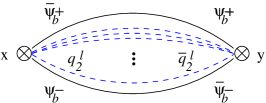
Figure 4: One of the four graphs of the correlator $\langle{\cal C}^{l}(x)\bar{\cal C}^{l}(y)\rangle$.

We show ${\cal O}(g^{2})$ nonrenormalization for ${\cal C}^{l}$ with $l=0$ for which $q_{2}$ exchanges are absent. The relevant propagators are

$$\langle v_{M}(x)v_{N}(y)\rangle=\frac{\eta_{MN}}{(2\pi)^{2}(x-y)^{2}},\qquad\langle q_{1}(x)\bar{q}_{1}(y)\rangle=\frac{1}{(2\pi)^{2}(x-y)^{2}}\,,$$ (7.2)

$$\langle\psi_{\alpha}(x)\bar{\psi}_{\beta}(y)\rangle=\frac{i}{2\pi}\frac{\rho^{M}_{\alpha\beta}(x-y)_{M}}{(x-y)^{2}}\,,$$ (7.3)

with $\eta_{MN}={\rm diag(+1,-1)}$, Pauli matrices $\rho^{M}(M=0,1)$ defined in appendix B, and defect coordinates $x,y$. The four-dimensional propagators in Eq. (7.2) are pinned to the defect. The Feynman rules for the vertices can be read off from the defect action in component form derived in appendix D.

First we note that, similar as in $\mathcal{N}=4$, $d=4$ SYM theory [44], there are no one-loop self-energy corrections to the defect fermionic propagator $\langle\bar{\psi}_{b}\psi_{b}\rangle$. Self-energy corrections involving a gaugino propagator are cancelled by those involving a $\psi^{q_{1}}$ propagator which is the fermion of the superfield $Q_{1}$. There are also self-energy graphs with $q_{1}$ and $\sigma$ propagators which arise from the ambient scalars coupling to the defect. These cancel each other, too.

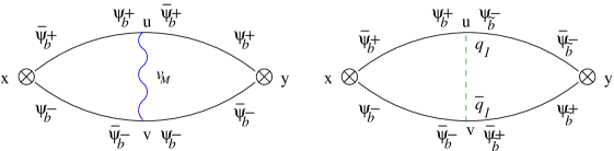
Figure 5: First order corrections to the correlator $\langle{\cal C}^{l}(x)\bar{\cal C}^{l}(y)\rangle$ for $l=0$.

However, we have two possible corrections from exchange graphs as shown in Fig. 5. Note that in Fig. 5, two different contributions to ${\cal C}^{l}$ ($l=0$) are depicted at the point $y$, which originate from different terms in the sum (7.1). These graphs include an ambient gauge boson exchange and an ambient scalar exchange. There is no $\sigma$ exchange contributing to the correlator $\langle{\cal C}^{l}(x){\cal C}^{l}(y)\rangle$ (for $l=0$). In fact, it may be shown that for each of the components of ${\cal C}^{\mu l}$, there is either a $\sigma$ or a $q_{1}$ exchange. For all of the components, the vector exchange is cancelled by one of these scalar exchanges while the other one vanishes.

For the gauge boson exchange in Fig. 5a we find the contribution

$$\frac{1}{2}\int d^{2}ud^{2}v\, \frac{\rho_{++}\cdot(x-u)}{2\pi(x-u)^{2}}(-\frac{1}{2}g\rho^{M}_{++})\frac{\eta_{MN}}{(2\pi)^{2}(u-v)^{2}}(-\frac{1}{2}g\rho^{N}_{--})\frac{\rho_{++}\cdot(u-y)}{2\pi(u-y)^{2}}$$

$$\times\frac{\rho_{--}\cdot(x-v)}{2\pi(x-v)^{2}}\frac{\rho_{--}\cdot(v-y)}{2\pi(v-y)^{2}}\,.$$ (7.4)

The overall factor $\frac{1}{2}$ comes from the definition $v_{M}=\frac{1}{\sqrt{2}}v^{\prime}_{M}$.

Let us now consider the contribution from the $q_{1}$ exchange in Fig. 5b which is given by

$$-\int d^{2}ud^{2}v\, \frac{\rho_{++}\cdot(x-u)}{2\pi(x-u)^{2}}(\frac{1}{2}ig)\frac{1}{(2\pi)^{2}(u-v)^{2}}(-\frac{1}{2}ig)\frac{\rho_{--}\cdot(u-y)}{2\pi(u-y)^{2}}$$

$$\times\frac{\rho_{--}\cdot(x-v)}{2\pi(x-v)^{2}}\frac{\rho_{++}\cdot(v-y)}{2\pi(v-y)^{2}}\,.$$ (7.5)

Note that the operator at the external point $y$ in the graph of Fig. 5b is the conjugate of the first term in Eq. (7.1) which leads to the minus sign in front of the integral in Eq. (7.5). In Fig. 5a both external vertices have a minus sign, whereas in Fig. 5b the vertices have opposite signs. Since $\eta_{MN}\rho^{M}_{++}\rho^{N}_{--}=2$, the vector exchange exactly cancels the contribution from the scalar exchange.

Nonrenormalization of correlators of ${\cal C}^{\mu l}$ with $l\geq 1$ is more difficult to show. As was shown for the operators ${\rm Tr\,}X^{k}$ in $\mathcal{N}=4$ super Yang-Mills theory [44, 45], there are no exchanges between the ambient propagators $\langle q_{2}(x)\bar{q}_{2}(y)\rangle$ within the correlator $\langle{\cal C}^{l}(x)\bar{\cal C}^{l}(y)\rangle$. However, one could think of a gauge boson exchange between a fermionic defect and a bosonic ambient propagator. If we do not work in Wess-Zumino gauge then there is an additional interaction of the defect fermions with a scalar $C$ which is the lowest component of the gauge superfield $V$. Keeping this in mind we expect that a CD exchange [44] cancels the above gauge boson exchange. This will be shown elsewhere.

7.2 Vanishing of odd correlators of the BPS primaries ${\cal C}^{\mu l}$

Another property of the BPS primaries ${\cal C}^{\mu l}$ is the vanishing of all $(2k+1)$-point functions ($k\in\mathbb{N}$). Only even $n$-point functions may differ from zero. On the gravity side this can be seen by studying once more the BI action of the probe D3-brane. Due to the expansion of the cosines of the angular fluctuations $\theta,\phi,\rho$, and $\chi$ in the determinant, the BI action contains only even powers of the fluctuations, see Eq. (3.5). This implies vanishing odd couplings for the Kaluza-Klein modes which, via the AdS/CFT correspondence, implies vanishing odd $n$-point functions on the field-theory side. In the dual conformal field theory these Kaluza-Klein modes correspond to the BPS primary operators ${\cal C}^{\mu l}$. Again we restrict to the component ${\cal C}^{l}\equiv{\cal C}^{1l}$.

On the field theory side too, one finds for instance that the three-point function $\langle{\cal C}^{l_{1}}(x){\cal C}^{l_{2}}(y){\cal C}^{l_{3}}(z)\rangle$ is absent. This is due to a global $U(1)$ symmetry of the action,

$$B \rightarrow e^{i\frac{\phi}{2}}B\,,\qquad\tilde{B}\rightarrow e^{i\frac{\phi}{2}}\tilde{B}\,,\qquad Q_{1}\rightarrow e^{-i\phi}Q_{1}\,,\qquad Q_{2}\rightarrow e^{i\phi}Q_{2}\,,$$ (7.6)

with all other fields being singlets under this symmetry. If we choose $\phi=\pi$ then ${\cal C}^{l}\rightarrow(e^{i\pi})^{l+1}{\cal C}^{l}$ and the three-point function transforms as

$$\langle{\cal C}^{l_{1}}(x){\cal C}^{l_{2}}(y){\cal C}^{l_{3}}(z)\rangle\rightarrow(-1)^{l_{1}+l_{2}+l_{3}+1}\langle{\cal C}^{l_{1}}(x){\cal C}^{l_{2}}(y){\cal C}^{l_{3}}(z)\rangle\,.$$ (7.7)

Since $l_{1}+l_{2}+l_{3}$ must be even, $(-1)^{l_{1}+l_{2}+l_{3}+1}=-1$ and $\langle{\cal C}^{l_{1}}(x){\cal C}^{l_{2}}(y){\cal C}^{l_{3}}(z)\rangle$ vanishes. Though we have restricted the discussion on ${\cal C}^{1l}$, the statement also holds for the other components. This is guaranteed by the fact that ${\cal C}^{\mu l}$ transforms as a vector under the $SO(4)$ R-symmetry group.

8 Conclusions and open questions

We have presented the action and some of the elementary properties of a defect conformal field theory describing intersecting D3-branes, including some aspects of the AdS/CFT dictionary. There remain many interesting open questions, of which we enumerate a few below.

The defect conformal field theory requires further field-theoretic analysis. One of the stranger features of this theory is that it contains massless two-dimensional scalars with (presumably) exactly marginal gauge, Yukawa, and scalar potential couplings. It is not at all obvious that one can construct a Hilbert space corresponding to operators with power law correlation functions, due to the logarithmic correlators of the two-dimensional scalars. It would be very interesting if one could show this to all orders in perturbation theory.

As a precursor to including gravity into the holographic map, it would be interesting to study the energy-momentum tensor of the defect conformal field theory in detail. We did not find any evidence of an enhancement of the two-dimensional $SO(2,2)$ global conformal symmetry to a full infinite-dimensional conformal symmetry on the two-dimensional defect. A study of the energy-momentum tensor would allow us to address this question conclusively at least from the field-theoretic side. For example, if an enhancement did indeed occur it should manifest itself in the form of a two-dimensional energy-momentum tensor which is holomorphically conserved.

Another question concerns the light-cone open string vacuum for D3-branes in the Penrose limit of the probe-supergravity background which we have considered. The operator proposed in [10] to correspond to the open string light-cone vacuum is not really a chiral primary and gives negative light-cone energy. This operator is precisely the one given in (6.1), and contains the dimensionless scalars which parameterize the Higgs branch. One might instead propose the operator ${\cal C}^{\mu l}$, with $P_{-}=\Delta-l=0$ as the dual of the light-cone vacuum, however this is only $1/4$ BPS and is in a non-trivial representation of the unbroken $SU(2)_{L}\times SU(2)_{R}$ R-symmetry. Presumably the subtleties regarding the light-cone vacuum are related to the quantum spreading over holomorphic embeddings $wy=c$ corresponding to the classical Higgs branch of the defect CFT. While the origin of this spreading is clear from the point of view of the dual defect CFT, and from the difficulties in finding localized supergravity solutions for intersecting D3-branes [22, 24, 23], they are not so clear from the point of view of a probe D3-brane embedded in the plane-wave or $AdS$ backgrounds.

Although there is presumably no fully localized supergravity solution for intersecting D3-branes, it would be surprising if there is no closed string string description, in which both stacks of D3-branes are replaced by geometry. The problem of finding a closed string description of the theory raises a closely related question of how new degrees of freedom appear when $1/N$ (or $g_{s}$) corrections are taken into account in probe-supergravity background which we have considered. In constructing the holographic dual of the defect CFT, we have fixed the number $N^{\prime}$ of D3-branes in one stack, while taking the number $N$ of D3-branes in the orthogonal stack to infinity. In this limit, the degrees of freedom on one four-dimensional part of the world volume of the defect become free. The remaining coupled degrees of freedom live on a four-dimensional world volume and a two-dimensional defect, which are the boundaries of $AdS_{5}$ and the embedded $AdS_{3}$ respectively. Because the defect degrees of freedom are in the fundamental representation, the genus expansion of Feynman diagrams resembles an open string world-sheet expansion. When $1/N$ corrections are taken into account, the decoupled degrees of freedom must somehow reappear. The defect degrees of freedom become bi-fundamental fields with respect to a $SU(N)\times SU(N^{\prime})$ gauge group. The genus expansion for Feynman diagrams of the theory can now be viewed as a closed string world-sheet expansion, where a new branch of the target space has opened up.

Finally, the string theory realization of the defect CFT leads one to expect that it exhibits S-duality. It would be very interesting to find some field theoretic evidence for this. In particular one would need to find the S-duals of the fundamental degrees of freedom localized at the intersection.

Acknowledgements

We are grateful to Glenn Barnich, Oliver DeWolfe, Dan Freedman, Ami Hanany, Robert Helling, Marc Henneaux, Andreas Karch, Neil Lambert, Joe Minahan, Carlos Nuñez, Volker Schomerus, David Tong, Paul Townsend and Jan Troost for useful discussions. The authors are particularly indebted to Robert Helling and to David Tong for helpful comments. The research of J.E., Z.G. and I.K. is funded by the DFG (Deutsche Forschungsgemeinschaft) within the Emmy Noether programme, grant ER301/1-2. N.R.C. is supported by the DOE under grant DF-FC02-94ER40818, the NSF under grant PHY-0096515 and NSERC of Canada.

Appendix

Appendix A Kinematics of 2d/4d defect conformal field theories

A.1 Conformal symmetry

Here we present some basic implications of conformal symmetry in a four-dimensional field theory with a two-dimensional defect.

Consider four-dimensional Euclidean space with a two-dimensional defect. The coordinates are given by $v_{\mu}=(\vec{z},\vec{x})$ where $v_{\mu}$ are the four-dimensional coordinates, $\vec{z}_{M}$ are the two defect coordinates and $\vec{x}_{\alpha}$ are the coordinates perpendicular to the defect. The conformal transformations which leave the defect invariant are given by translations and rotations within the defect plane, rotations in the plane perpendicular to the defect and by inversions $v_{\mu}\rightarrow v_{\mu}/v^{2}$. The conformal group is given by $SO(3,1)\times SO(2)$. Under these transformations we have for two points $v$, $v^{\prime}$

$$(v-v^{\prime})^{2}\rightarrow\frac{(v-v^{\prime})^{2}}{\Omega(v)\Omega(v^{\prime})}\,,\quad\vec{x}_{\alpha}\rightarrow\frac{\vec{x}_{\alpha}}{\Omega(v)}\,\quad\vec{x}^{\prime}_{\alpha}\rightarrow\frac{\vec{x}^{\prime}_{\alpha}}{\Omega(v^{\prime})}\,.$$ (A.1)

Hence there is a dimensionless coordinate invariant of the form

$$\xi=\frac{(v-v^{\prime})^{4}}{(\vec{x}\cdot\vec{x})(\vec{x}^{\prime}\cdot\vec{x}^{\prime})}\,.$$ (A.2)

Note that in the defect plane, we have only a global conformal symmetry associated with the Virasoro generators $L_{-1}$, $L_{0}$ and $L_{1}$. One may wonder if there is an accidental two-dimensional local conformal symmetry giving rise to a Virasoro algebra. This is however not the case: A necessary condition for the existence of a Virasoro algebra is the existence of a two-dimensional conserved local energy-momentum tensor. This requirement is not satisfied in the situation considered here since only the four-dimensional energy-momentum tensor of the combined four-dimensional and two-dimensional action contributions, given by

$$T_{\mu\nu}(v)\,=\,T^{\rm bulk}{}_{\mu\nu}(v)\,+\,T^{\rm def}{}_{MN}(\vec{z})\,\delta_{M(\mu}\delta_{\nu)N}\,\delta^{(2)}(\vec{x})\,\,,$$ (A.3)

is conserved, $\partial_{\mu}T_{\mu\nu}=0$. Note that this energy-momentum tensor is in agreement with the $(2,2)$ supercurrent (E.4) since from (A.3) we obtain by integration over $x$

$${\cal T}_{MN}(z)=\int\!d^{2}x\,T^{\rm bulk}{}_{MN}(x,z)\,+\,T^{\rm def}{}_{MN}(z)\,,$$ (A.4)

which is contained as a component in ${\cal J}_{M}$ given by (E.4). ${\cal T}_{MN}(z)$ satisfies $\partial^{z}{}_{M}{\cal T}_{MN}(z)=0$. Nevertheless it is not a local traceless two-dimensional energy-momentum tensor.

For a quasi-primary scalar operator of dimension $\Delta$ close to the defect we have a one-point function

$$\langle{\cal O}(v)\rangle\,=\,\frac{A_{\cal O}}{(\vec{x}\cdot\vec{x})^{\Delta/2}}\,.$$ (A.5)

Near to the defect we have a boundary operator expansion of the bulk operators in terms of the defect operators, which reads

$${\cal O}(v)\,=\,\sum\limits_{n}\frac{B_{{\cal O},\hat{\cal O}_{n}}}{(\vec{x}\cdot\vec{x})^{(\Delta-\hat{\Delta}_{n})/2}}\,\hat{{\cal O}}_{n}(\vec{z})\,.$$ (A.6)

This gives rise to a bulk-defect correlator

$$\langle{{\cal O}}(v)\hat{{\cal O}}_{n}(\vec{z}^{\prime})\rangle\,=\,\frac{B_{{\cal O},\hat{{\cal O}}_{n}}}{(\vec{x}\cdot\vec{x})^{(\Delta-\hat{\Delta}_{n})/2}(v-v^{\prime})^{2\hat{\Delta}_{n}}}\,,\quad(v-v^{\prime})_{\mu}=(\vec{x},\vec{z}-\vec{z}^{\prime}).$$ (A.7)

For two operators of dimension $\hat{\Delta}_{n}$ on the defect, this expression reduces to

$$\langle\hat{{\cal O}}_{n}(\vec{z})\hat{{\cal O}}_{n}(\vec{z}^{\prime})\rangle\,=\,\frac{B_{{\hat{{\cal O}}_{n}},\hat{{\cal O}}_{n}}}{(\vec{z}-\vec{z}^{\prime})^{2\hat{\Delta}_{n}}}\,$$ (A.8)

as expected.

A.2 SUGRA calculation of one-point functions and bulk-defect two point functions

We now compute the space-time dependence of the bulk one-point and the bulk-defect two-point function using holographic methods and show that their structure agrees with the general results obtained from conformal invariance in section A.1. The one-point function of the bulk operator ${{\cal O}}_{\Delta}$ is the integral of the standard bulk-boundary propagator in $AdS_{5}$ [32] over the $AdS_{3}$ subspace. We find

$$\langle{{\cal O}}_{\Delta}(\vec{x},\vec{z})\rangle =\int\frac{dwd\vec{w}^{2}}{w^{3}}\frac{\Gamma(\Delta)}{\pi^{2}\Gamma(\Delta-2)}\left(\frac{w}{w^{2}+\vec{x}^{2}+(\vec{w}-\vec{z})^{2}}\right)^{\Delta}$$

$$=\frac{1}{|\vec{x}|^{\Delta}}\frac{\Gamma(\frac{1}{2}\Delta+1)\Gamma(\frac{1}{2}\Delta-1)}{2\pi\,\Gamma(\Delta-2)\,(\Delta-1)}\,,$$ (A.9)

which converges for $\Delta>2$. The scaling behaviour $|\vec{x}|^{-\Delta}$ has been expected from the structure of the one-point function (A.5) on the CFT side. Note that the DBI action (4.4) of the D3-brane probe determines the scale dependence on $N$ of the correlation functions of defect and bulk operators $\hat{{\cal O}}_{\hat{\Delta}}$ and ${{\cal O}}_{\Delta}$.

The two-point function $\langle{{\cal O}}_{\Delta}(\vec{x},\vec{z})\hat{{\cal O}}_{\hat{\Delta}}(0)\rangle$ is the integral over the product of the bulk-boundary propagators $K_{\Delta}\big{(}w,(\vec{x},\vec{z}),(\vec{0},\vec{w})\big{)}$ and $K_{\hat{\Delta}}\big{(}w,(\vec{0},\vec{w}),(\vec{0},\vec{0})\big{)}$ ,

$$\langle{{\cal O}}_{\Delta}(\vec{x},\vec{z})\hat{{\cal O}}_{\hat{\Delta}}(\vec{0})\rangle=\frac{1}{N^{1/2}}\frac{\Gamma(\Delta)}{\pi^{2}\Gamma(\Delta-2)}\frac{\Gamma(\hat{\Delta})}{\pi\Gamma(\hat{\Delta}-1)}J(\vec{x},\vec{z};\Delta,\hat{\Delta})$$ (A.10)

with the integral

$$J(\vec{x},\vec{z};\Delta,\hat{\Delta}) =\int\frac{dwd\vec{w}^{2}}{w^{3}}\left(\frac{w}{w^{2}+\vec{x}^{2}+(\vec{w}-\vec{z})^{2}}\right)^{\Delta}\left(\frac{w}{w^{2}+\vec{w}^{2}}\right)^{\hat{\Delta}}\,$$

$$=\frac{1}{(\vec{x}^{2}+\vec{z}^{2})^{\Delta}}\int dw^{\prime}d\vec{w}^{\prime 2}\,w^{\prime\hat{\Delta}-3}\left(\frac{w^{\prime}}{w^{\prime 2}+\vec{x}^{\prime 2}+(\vec{w}^{\prime}-\vec{z}^{\prime})^{2}}\right)^{\Delta}\,.$$ (A.11)

In the last line we made use of the inversion trick [32] by defining

$$(w^{\prime},0,\vec{w}^{\prime})=\frac{1}{w^{2}+\vec{w}^{2}}(w,0,\vec{w}),\qquad(\vec{x}^{\prime},\vec{z}^{\prime})=\frac{1}{\vec{x}^{2}+\vec{z}^{2}}(\vec{x},\vec{z})\,.$$ (A.12)

As in [8], we rescale $\vec{w}^{\prime}=\vec{z}^{\prime}+\sqrt{\vec{x}^{\prime 2}+w^{\prime 2}}\vec{v}$ and $w^{\prime}=|\vec{x}^{\prime}|u$ and find

$$J(\vec{x},\vec{z};\Delta,\hat{\Delta}) =\frac{1}{(\vec{x}^{2}+\vec{z}^{2})^{\hat{\Delta}}|\vec{x}|^{\Delta-\hat{\Delta}}}\int du\frac{u^{\hat{\Delta}-3+\Delta}}{(1+u^{2})^{\Delta-2}}\int d\vec{v}^{2}\frac{1}{(1+\vec{v}^{2})^{\Delta}}$$

$$=\frac{1}{(\vec{x}^{2}+\vec{z}^{2})^{\hat{\Delta}}|\vec{x}|^{\Delta-\hat{\Delta}}}\frac{\pi}{2(\Delta-1)}\frac{\Gamma[\frac{1}{2}(\Delta-\hat{\Delta})]\Gamma[\frac{1}{2}(\Delta+\hat{\Delta})]}{\Gamma[\Delta-2]}\,.$$ (A.13)

This converges for $\Delta>\hat{\Delta}$. The scaling $1/((\vec{x}^{2}+\vec{z}^{2})^{\hat{\Delta}}|\vec{x}|^{\Delta-\hat{\Delta}})$ agrees with the behaviour of the two-point function fixed by conformal invariance, cf. Eq. (A.7).

The defect-defect correlator $\langle\hat{{\cal O}}_{\hat{\Delta}}(\vec{z})\hat{{\cal O}}_{\hat{\Delta}}(\vec{0})\rangle$ for a defect operator $\hat{{\cal O}}_{\hat{\Delta}}$ is given by Eq. (17) in [32] with $d=2$ and is independent of $N$. Let us stress again that none of the above correlators depends on $\lambda$ in the strong coupling regime.

Appendix B Multiplets in $(2,2),d=2$ superspace

In order to fix the notation we briefly summarize the component expansions of the superfields in $(2,2),d=2$ superspace which can be found in [33], for instance. We use chiral coordinates $y^{0},y^{1},\theta^{\pm},\bar{\theta}^{\pm}$ which are related to the superspace coordinates $x^{0},x^{1},\theta^{\pm},\bar{\theta}^{\pm}$ by

$$y^{M} =x^{M}+i\theta^{+}\rho^{M}_{11}\bar{\theta}^{+}+i\theta^{-}\rho^{M}_{22}\bar{\theta}^{-}$$

$$=x^{M}+i\theta^{+}\bar{\theta}^{+}+(-1)^{M}i\theta^{-}\bar{\theta}^{-}\,,\qquad M=0,1\,,$$ (B.1)

where we use the Pauli matrices

$$\rho^{0}\equiv\sigma^{0}=\begin{pmatrix}1&0\\ 0&1\end{pmatrix},\,\rho^{1}\equiv\sigma^{3}=\begin{pmatrix}1&0\\ 0&-1\end{pmatrix},\,\rho^{2}\equiv\sigma^{2}=\begin{pmatrix}0&-i\\ i&0\end{pmatrix},\,\rho^{3}\equiv\sigma^{1}=\begin{pmatrix}0&1\\ 1&0\end{pmatrix}.$$ (B.2)

Expansions of (2,2) superfields can be obtained by dimensional reduction of $\mathcal{N}=1,d=4$ superfields in the $2$ and $3$ direction and defining $\theta^{+}\equiv\theta^{1}=\theta_{2}$ and $\theta^{-}\equiv\theta^{2}=-\theta_{1}$. In this way we find the expansions of the chiral and the vector multiplet in Wess-Zumino gauge,

$$\Phi(y,\theta^{\pm}) =\phi+\sqrt{2}\theta^{+}\psi_{+}+\sqrt{2}\theta^{-}\psi_{-}-2\theta^{+}\theta^{-}F$$ (B.3)

$$V(y,\theta^{\pm},\bar{\theta}^{\pm}) =\,\,\theta^{-}\bar{\theta}^{-}(v_{0}-v_{1})+\theta^{+}\bar{\theta}^{+}(v_{0}+v_{1})-\theta^{-}\bar{\theta}^{+}\sigma-\theta^{+}\bar{\theta}^{-}\bar{\sigma}$$

$$\quad+i\sqrt{2}\theta^{-}\theta^{+}(\bar{\theta}^{-}\bar{\lambda}_{-}+\bar{\theta}^{+}\bar{\lambda}_{+})+i\sqrt{2}\bar{\theta}^{+}\bar{\theta}^{-}(\theta^{-}\lambda_{-}+\theta^{+}\lambda_{+})$$ (B.4)

$$\quad+2\theta^{-}\theta^{+}\bar{\theta}^{+}\bar{\theta}^{-}(D-i\partial^{M}v_{M})\,.$$

The scalar $\sigma$ is complex and is defined in terms of the components $v_{1}$ and $v_{2}$ of the dimensionally reduced four-vector $v_{\mu}$ by $\sigma\equiv v_{3}+iv_{2}$. For the (abelian) twisted chiral superfield $\Sigma(y,\theta^{\pm},\bar{\theta}^{\pm})\equiv\bar{D}_{+}D_{-}V(y,\theta^{\pm},\bar{\theta}^{\pm})$ we find the expansion

$$\Sigma(y,\theta^{\pm},\bar{\theta}^{\pm})= \,\sigma+i\sqrt{2}\theta^{+}\bar{\lambda}_{+}-i\sqrt{2}\bar{\theta}^{-}\lambda_{-}+2\theta^{+}\bar{\theta}^{-}(D-if_{01})+2i\bar{\theta}^{-}\theta^{-}(\partial_{0}-\partial_{1})\sigma$$

$$-2\sqrt{2}\bar{\theta}^{-}\theta^{-}\theta^{+}(\partial_{0}-\partial_{1})\bar{\lambda}_{+}\,.$$ (B.5)

Appendix C Decomposing the $\mathcal{N}=2$, $d=4$ vector multiplet under $(2,2)$, $d=2$ supersymmetry

We start from the decomposition of the vector multiplet $\Psi$ under $\mathcal{N}=1$, $d=4$ which is given by an expansion in $\theta_{(2)}$ [47],

$$\Psi(\tilde{y},\theta_{(1)},\theta_{(2)})=\Phi^{\prime}(\tilde{y},\theta_{(1)})+i\sqrt{2}\theta^{\alpha}_{(2)}W^{\prime}_{\alpha}(\tilde{y},\theta_{(1)})+\theta_{(2)}\theta_{(2)}G^{\prime}(\tilde{y},\theta_{(1)})\,\,,$$ (C.1)

where $\Phi^{\prime}$, $W^{\prime}_{\alpha}$, and $G^{\prime}$ are chiral, vector, and auxiliary $\mathcal{N}=1$ multiplets, respectively. The superfield $\Psi$ is a function of the coordinate $\tilde{y}^{\mu}$ which is related to $x^{\mu}$ by

$$\tilde{y}^{\mu}=x^{\mu} +i\theta^{+}\sigma^{\mu}_{11}\bar{\theta}^{+}+i\theta\!\!\!/^{-}\sigma^{\mu}_{21}\bar{\theta}^{+}+i\theta^{+}\sigma^{\mu}_{12}\bar{\theta}\!\!\!/^{-}+i\theta\!\!\!/^{-}\sigma^{\mu}_{22}\bar{\theta}\!\!\!/^{-}$$

$$+i\bar{\theta}^{-}\sigma^{\mu}_{22}\theta^{-}+i\theta\!\!\!/^{+}\sigma^{\mu}_{12}\theta^{-}+i\bar{\theta}^{-}\sigma^{\mu}_{21}\bar{\theta}\!\!\!/^{+}+i\theta\!\!\!/^{+}\sigma^{\mu}_{11}\bar{\theta}\!\!\!/^{+}\,,$$ (C.2)

where $\sigma^{0}$ is the identity matrix and $\sigma^{a}$ ($a=1,2,3$) are the Pauli matrices.

Our goal is to find an expression for $\Psi$ in terms of $(2,2)$, $d=2$ multiplets,

$$\Psi\equiv\Psi|_{\theta\!\!\!/=\bar{\theta}\!\!\!/=0}+\theta\!\!\!/^{+}(D\!\!\!\!/\,_{+}\Psi)|_{\theta\!\!\!/=\bar{\theta}\!\!\!/=0}+\theta\!\!\!/^{-}(D\!\!\!\!/\,_{-}\Psi)|_{\theta\!\!\!/=\bar{\theta}\!\!\!/=0}+\theta\!\!\!/^{+}\theta\!\!\!/^{-}(D\!\!\!\!/\,_{+}D\!\!\!\!/\,_{-}\Psi)|_{\theta\!\!\!/=\bar{\theta}\!\!\!/=0}\,,$$ (C.3)

with $\theta\!\!\!/=(\theta\!\!\!/^{+},\theta\!\!\!/^{-})$. In order to find the coefficients of this expansion, we substitute the component expansions of $\Phi^{\prime}$, $W^{\prime}_{\alpha}$ and $G^{\prime}$ in (C.1) and use the coordinates ($\tilde{y}$, $\theta^{\pm}$, $\theta\!\!\!/^{\pm}$, $\bar{\theta}^{\pm}$, $\bar{\theta}\!\!\!/^{\pm}$) as defined in (5.1.1). We find

$$\Psi= \,\phi^{\prime}+\sqrt{2}\theta^{+}\psi^{\prime}_{+}+\sqrt{2}\theta\!\!\!/^{-}\psi^{\prime}_{-}-2\theta^{+}\theta\!\!\!/^{-}F^{\prime}$$

$$+i\sqrt{2}\bar{\theta}^{-}\left(-i\lambda^{\prime}_{-}+\theta^{+}D^{\prime}+\theta^{+}(f^{\prime}_{12}-if^{\prime}_{03})+\theta\!\!\!/^{-}(f^{\prime}_{02}-f^{\prime}_{32}+if^{\prime}_{10}-if^{\prime}_{13})\right.$$

$$\left.\qquad\qquad-2\theta^{+}\theta\!\!\!/^{-}(\partial_{1}\bar{\lambda}^{\prime+}+i\partial_{2}\bar{\lambda}^{\prime+}+\partial_{0}\bar{\lambda}^{\prime-}-\partial_{3}\bar{\lambda}^{\prime-})\right)$$

$$+i\sqrt{2}\theta\!\!\!/^{+}\left(-i\lambda^{\prime}_{+}-\theta\!\!\!/^{-}D^{\prime}-\theta^{+}(f^{\prime}_{02}+f^{\prime}_{32}-if^{\prime}_{10}-if^{\prime}_{13})+\theta\!\!\!/^{-}(f^{\prime}_{21}+if^{\prime}_{03})\right.$$ (C.4)

$$\left.\qquad\qquad-2\theta^{+}\theta\!\!\!/^{-}(\partial_{1}\bar{\lambda}^{\prime-}-i\partial_{2}\bar{\lambda}^{\prime-}+\partial_{0}\bar{\lambda}^{\prime+}+\partial_{3}\bar{\lambda}^{\prime+})\right)$$

$$-2\theta\!\!\!/^{+}\bar{\theta}^{-}\left(F^{\prime*}-i\sqrt{2}\theta^{+}(\partial_{1}\bar{\psi}^{\prime-}-i\partial_{2}\bar{\psi}^{\prime-}+\partial_{0}\bar{\psi}^{\prime+}+\bar{\partial}_{3}\psi^{\prime+})+2\theta^{+}\theta\!\!\!/^{-}\square_{4}\phi^{\prime*}\right)\,.$$

Note that all fields are functions of $\tilde{y}$ and we have to expand this expression such that all fields become functions of the chiral coordinates $y^{M}=x^{M}+i\theta^{+}\bar{\theta}^{+}+(-1)^{M}i\theta^{-}\bar{\theta}^{-}\,(M=0,3)$. Evaluating $\Psi$, $D\!\!\!\!/\,_{+}\Psi$, and $D\!\!\!\!/\,_{-}\Psi$ at $\theta\!\!\!/^{+}={\theta\!\!\!/^{-}=0}$ we obtain

$$\Psi|_{\theta\!\!\!/=0} =-i\Sigma\,,$$

$$\quad(D\!\!\!\!/\,_{+}\Psi)|_{\theta\!\!\!/=0} =\bar{D}_{+}\left(\bar{\Phi}-\partial_{\bar{x}}V\right)\,,\quad(D\!\!\!\!/\,_{-}\Psi)|_{\theta\!\!\!/=0}=D_{-}\left(\Phi-\partial_{x}V\right)\,,$$ (C.5)

where $\partial_{x}\equiv\partial_{1}+i\partial_{2}$ is the derivative transverse to the defect. Here we defined the (unprimed) components of the (2,2) superfields $\Sigma$, $\Phi$, and $V$ in terms of the (primed) components of the $\mathcal{N}=1$, $d=4$ superfield $\Phi^{\prime}$ and $W^{\prime}_{\alpha}$ by

$$\sigma\equiv i\phi^{\prime},\quad\bar{\lambda}_{+}\equiv\psi^{\prime}_{+},\quad\lambda_{-}\equiv-\lambda^{\prime}_{-},\quad D\equiv\frac{1}{\sqrt{2}}(D^{\prime}+f^{\prime}_{12}),\quad f_{03}\equiv\frac{1}{\sqrt{2}}f^{\prime}_{03}\,,$$

$$\phi{}\equiv\frac{1}{\sqrt{2}}(v^{\prime}_{1}+iv^{\prime}_{2}),\quad\bar{\psi}_{+}\equiv\lambda^{\prime}_{+},\quad\psi_{-}\equiv\psi^{\prime}_{-},\quad F{}\equiv F^{\prime}$$ (C.6)

If we substitute the coefficients (C.5) back into the expansion (C.3) of $\Psi$, we find the decomposition (5.10).

The appearance of $f^{\prime}_{12}$ in the definition (C.6) of the auxiliary field $D$ is required by $(2,0)\subset(2,2)$ supersymmetry. Consider the (2,0) supersymmetry transformation rules for the spinor component $\lambda^{\prime+}$, the auxiliary field $D^{\prime}$, and the component $f^{\prime}_{12}$ given by

$$\delta_{\epsilon}\lambda^{\prime+} =i\epsilon^{+}(D^{\prime}+f^{\prime}_{12}-if^{\prime}_{03})$$

$$\delta_{\epsilon}D^{\prime} =\bar{\epsilon}^{+}(\partial_{0}-\partial_{3})\lambda^{\prime+}-\epsilon^{+}(\partial_{0}-\partial_{3})\bar{\lambda}^{\prime+}-\bar{\epsilon}^{+}(\partial_{1}-i\partial_{2})\lambda^{\prime-}-\epsilon^{+}(\partial_{1}-i\partial_{2})\bar{\lambda}^{\prime-}$$

$$\delta_{\epsilon}f^{\prime}_{12} =\epsilon^{+}(\partial_{1}-i\partial_{2})\bar{\lambda}^{\prime-}+\bar{\epsilon}^{+}(\partial_{1}-i\partial_{2})\lambda^{\prime-}\,.$$ (C.7)

Of particular interest in Eq. (C) are the non-standard terms appearing in the variations of $\lambda^{\prime+}$ and $D^{\prime}$ involving transverse derivatives, $\partial_{2}$ and $\partial_{1}$. Note that in dimensional reduction these terms would have simply been set to zero. The susy variation of $f^{\prime}_{12}$ in $\delta_{\epsilon}D\equiv\textstyle\frac{1}{\sqrt{2}}\delta_{\epsilon}(D^{\prime}+f^{\prime}_{12})$ precisely cancels the non-standard terms in the variation of the auxiliary field $D^{\prime}$. This leads to the familiar (2,0) susy variation for $D$,

$$\delta_{\epsilon}D =\bar{\epsilon}^{+}(\partial_{0}-\partial_{3})\lambda^{+}-\epsilon^{+}(\partial_{0}-\partial_{3})\bar{\lambda}^{+}\,.$$ (C.8)

Appendix D Impurity action in component form

In this appendix we derive the component expansion of the impurity action in the decoupling limit which is given by

$$S^{\rm dec}_{D3-D3^{\prime}}\equiv \,S_{\rm kin}+S_{\rm superpot}$$

$$= \int d^{2}zd^{4}\theta\left(\bar{B}e^{gV}B+{\tilde{B}}e^{-gV}\bar{\tilde{B}}\right)+\,\frac{ig}{{2}}\int d^{2}zd^{2}\theta(\tilde{B}Q_{1}B)+c.c.$$ (D.1)

with $d^{4}\theta=\frac{1}{4}d\theta^{+}d\theta^{-}d\bar{\theta}^{+}d\bar{\theta}^{-}$ and $d^{2}\theta=\frac{1}{2}d\theta^{+}d\theta^{-}$. Using the following expansions for the (2,2) superfields $B$, $\tilde{B}$, $Q_{1}$,

$$B =b+\sqrt{2}\theta^{+}\psi^{b}_{+}+\sqrt{2}\theta^{-}\psi^{b}_{-}-2\theta^{+}\theta^{-}F^{b}$$

$$\tilde{B} =\tilde{b}+\sqrt{2}\theta^{+}\psi^{\tilde{b}}_{+}+\sqrt{2}\theta^{-}\psi^{\tilde{b}}_{-}-2\theta^{+}\theta^{-}F^{\tilde{b}}$$ (D.2)

$$Q_{1} =q_{1}+\sqrt{2}\theta^{+}\psi^{q_{1}}_{+}+\sqrt{2}\theta^{-}\psi^{q_{1}}_{-}-2\theta^{+}\theta^{-}F^{q_{1}}$$

as well as Eq. (B.4) for $V$, the impurity action can be expanded as

$$S_{\rm kin} =\int d^{2}z\big{(}\bar{F}^{b}F^{b}-|D_{M}b|^{2}+i\bar{\psi}^{b}_{-}(D_{0}+D_{1})\psi^{b}_{-}+i\bar{\psi}^{b}_{+}(D_{0}-D_{1})\psi^{b}_{+}$$

$$\quad-\frac{g}{2}(\bar{\psi}^{b}_{-}\sigma\psi^{b}_{+}+\bar{\psi}^{b}_{+}\bar{\sigma}\psi^{b}_{-})+\frac{ig}{{2}}(b\bar{\psi}^{b}_{+}\bar{\lambda}_{-}-b\bar{\lambda}_{+}\bar{\psi}^{b}_{-}-\bar{b}\lambda_{-}\psi^{b}_{+}+\bar{b}\lambda_{+}\psi^{b}_{-})$$

$$\quad+\frac{1}{2}(gD-\frac{1}{2}g_{YM}^{2}\bar{\sigma}\sigma)\bar{b}b\big{)}+(B\rightarrow\tilde{B},g\rightarrow-g)$$ (D.3)

$$S_{\rm superpot} =\frac{ig}{{2}}\int d^{2}z\big{(}\tilde{b}F^{q_{1}}b+\tilde{b}\psi^{q_{1}}_{-}\psi^{b}_{+}+{\psi}^{\tilde{b}}_{+}\psi^{q_{1}}_{-}b+F^{\tilde{b}}q_{1}b+\psi^{\tilde{b}}_{-}\psi^{q_{1}}_{+}b+\psi_{-}^{\tilde{b}}q_{1}\psi^{b}_{+}$$

$$\quad+\tilde{b}q_{1}F^{b}+\psi_{+}^{\tilde{b}}q_{1}\psi_{-}^{b}+\tilde{b}\psi_{+}^{q_{1}}\psi_{-}^{b}\big{)}+c.c.$$ (D.4)

where we used the covariant derivative $D_{M}=\partial_{M}+\textstyle\frac{i}{2}gv_{M}$ $(M=0,1)$.

For the ambient action we have the standard component expansion of $\mathcal{N}=4,d=4$ SYM. Some of the components of the $\mathcal{N}=4$ ambient vector field, which we gather in the (2,2) fields $V$ and $Q_{1}$, couple to the impurity. The components of $V$ and $Q_{1}$ are related to the components of the $\mathcal{N}=1,d=4$ superfields $V^{\prime}$, $\Phi^{\prime}$, $\Phi^{\prime}_{1}$, and $\Phi^{\prime}_{2}$, which form the $\mathcal{N}=4$ vector multiplet, by

$$\sigma\equiv i\phi^{\prime},\quad\bar{\lambda}_{+}\equiv\psi^{\prime}_{+},\quad\lambda_{-}\equiv-\lambda^{\prime}_{-},\quad D\equiv\frac{1}{\sqrt{2}}(D^{\prime}+f^{\prime}_{32}),\quad f_{01}\equiv\frac{1}{\sqrt{2}}f^{\prime}_{01}\,,$$

$$q_{i}\equiv\phi^{\prime}_{i},\quad\psi^{q_{i}}_{\pm}=\psi^{\prime\phi_{i}}_{\pm},\quad F^{q_{i}}\equiv F^{\prime\phi_{i}}\qquad(i=1,2)\,.$$ (D.5)

Appendix E Quantum conformal invariance

Here we give an argument that the action given by (5.2), (5.2) and (5.2) does not receive quantum corrections, such that it remains conformal to all orders in perturbation theory. This argument is analogous to the discussion of the 3d/4d case in [9], where more details on the renormalization procedure may be found.

The argument for excluding possible quantum breakings of conformal symmetry by defect operators relies on considering the (2,2) supercurrent and its possible anomalies, and by making the assumption that $(4,4)$ supersymmetry is preserved by the quantum corrections. We begin by recalling the situation in $\mathcal{N}=1$, $d=4$ theories. In this case there is a supercurrent $J_{\dot{\alpha}\beta}=\sigma^{\mu}{}_{\dot{\alpha}\beta}J_{\mu}$, which has the R current, the supersymmetry currents and the energy-momentum tensor among its components. Potential superconformal anomalies may be written in the form

$$\bar{D}^{\dot{\alpha}}J_{\dot{\alpha}\beta}\,=\,D_{\beta}S\,,$$ (E.1)

with $S$ a chiral superfield. When $S=0$, superconformal symmetry is conserved.

By standard dimensional reduction to $(2,2)$ supersymmetry in two dimensions, we obtain from (E.1), as shown in [48],

$$(\gamma^{M})_{A}{}^{B}\bar{D}_{B}{\cal J}_{M}\,=D_{A}\,{\cal S}\,,$$ (E.2)

where $M=\{1,2\}$, $A,B=\{+,-\}$, $\gamma^{M}=\{\sigma^{1},i\sigma^{2}\}$ are the two-dimensional gamma matrices, ${\cal J}_{M}$ is the two-dimensional $(2,2)$ supercurrent and the possible conformal anomaly is given by the $(2,2)$ chiral superfield ${\cal S}$. ${\cal J}_{M}$ contains the 2d R-current, the four $(2,2)$ supersymmetry currents and the 2d energy-momentum tensor.

For 2d/4d models like the one given by (5.2), (5.2) and (5.2), the classically conserved two-dimensional supercurrent is given by

$${\cal J}_{M}(z)\,=\,{\cal J}^{\rm def}{}_{M}(z)\,+\,\int\!d^{2}x\;{\cal J}^{\rm bulk,1}{}_{M}(x,z)\,+\,\int\!d^{2}y\;{\cal J}^{\rm bulk,2}{}_{M}(y,z)\,.$$ (E.3)

Let us first consider possible defect operator contributions to the anomaly ${\cal S}$, which have to be gauge invariant and of dimension 1. The possible defect contributions to the anomaly ${\cal S}$ are given by

$${\cal S}_{D}\,=\,{\rm Tr}\,[u\,\bar{D}^{+}\bar{D}^{-}(e^{-\cal V}\bar{B}e^{V}B+e^{-V}\bar{\tilde{B}}e^{\cal V}\tilde{B})\,+\,\,v\,(B\tilde{B}Q_{1}-\tilde{B}BS_{1})\,]\,.$$ (E.4)

It is important to note that there is no gauge anomaly term contributing to this equation, since ${\rm Tr\,}\Sigma$ or ${\rm Tr\,}\Omega$, which would have the right dimension, are twisted chiral and not chiral. $u$ and $v$ are coefficients which may be calculated perturbatively. They are related to the $\beta$ and $\gamma$ functions. From the standard supersymmetric non-renormalization theorem we know that $v=0$ since the corresponding operator is chiral. $u$ may be non-zero in a general $(2,2)$ supersymmetric gauge theory. However $u$ and $v$ are related by $(4,4)$ supersymmetry. Therefore if we assume that $(4,4)$ supersymmetry is preserved upon quantization, $v=0$ also implies $u=0$. Thus there are no defect contributions breaking conformal symmetry.

We may also show that there are no contributions from four-dimensional operators to the conformal anomaly ${\cal S}$. Such terms would have to originate from bulk action counterterms which asymptotically fall off with the distance from the boundary. Asymptotically such anomaly contributions would be of the form

$${\cal S}_{B}\,\sim\,\int\!d^{2}w\,|w|^{-s_{1}}\Lambda^{t_{1}}{\cal O}_{1}(w,z)\,+\,\int\!d^{2}y\,|y|^{-s_{2}}\Lambda^{t_{2}}\,{\cal O}_{2}(y,z)\,,$$ (E.5)

with $\Lambda$ a regulator scale, and $s_{i}\geq 2$, $t_{i}\geq 0$ for $i=1,2$. However there are no such operators available in the theory. From dimensional analysis, only ${\rm Tr\,}\Sigma$ or ${\rm Tr\,}\Omega$ would be possible for ${\cal O}_{1}$ or ${\cal O}_{2}$, respectively, but again these are twisted chiral and not chiral. Therefore we conclude that there a no terms breaking $SO(2,2)$ conformal invariance, such that the theory is conformal to all orders in perturbation theory.

References

• [1] J. L. Cardy, “Conformal Invariance And Surface Critical Behavior,” Nucl. Phys. B 240 (1984) 514.
• [2] D. M. McAvity and H. Osborn, “Conformal field theories near a boundary in general dimensions,” Nucl. Phys. B 455 (1995) 522 [arXiv:cond-mat/9505127].
• [3] S. Sethi, “The matrix formulation of type IIB five-branes,” Nucl. Phys. B 523 (1998) 158 [arXiv:hep-th/9710005].
• [4] O. J. Ganor and S. Sethi, “New perspectives on Yang-Mills theories with sixteen supersymmetries,” JHEP 9801 (1998) 007 [arXiv:hep-th/9712071].
• [5] A. Kapustin and S. Sethi, “The Higgs branch of impurity theories,” Adv. Theor. Math. Phys.  2 (1998) 571 [arXiv:hep-th/9804027].
• [6] J. M. Maldacena, “The large N limit of superconformal field theories and supergravity,” Adv. Theor. Math. Phys.  2, 231 (1998) [Int. J. Theor. Phys.  38, 1113 (1999)] [arXiv:hep-th/9711200].
• [7] A. Karch and L. Randall, “Open and closed string interpretation of SUSY CFT’s on branes with boundaries,” JHEP 0106 (2001) 063 [arXiv:hep-th/0105132].
A. Karch and L. Randall, “Locally localized gravity,” JHEP 0105, 008 (2001) [arXiv:hep-th/0011156].
A. Karch and L. Randall, “Localized gravity in string theory,” Phys. Rev. Lett.  87 (2001) 061601 [arXiv:hep-th/0105108].
• [8] O. DeWolfe, D.Z. Freedman and H. Ooguri, “Holography and defect conformal field theories,” Phys. Rev. D 66, 025009 (2002) [arXiv:hep-th/0111135].
• [9] J. Erdmenger, Z. Guralnik and I. Kirsch, “Four-dimensional superconformal theories with interacting boundaries or defects,” Phys. Rev. D 66 (2002) 025020 [arXiv:hep-th/0203020].
• [10] K. Skenderis and M. Taylor, “Branes in AdS and pp-wave spacetimes,” JHEP 0206 (2002) 025 [arXiv:hep-th/0204054].
• [11] M. Porrati, “Mass and gauge invariance. IV: Holography for the Karch-Randall model,” Phys. Rev. D 65 (2002) 044015 [arXiv:hep-th/0109017].
• [12] A. Fayyazuddin, “Supersymmetric webs of D3/D5-branes in supergravity,” [arXiv:hep-th/0207129].
• [13] M. J. Duff, J. T. Liu and H. Sati, “Complementarity of the Maldacena and Karch-Randall pictures,” [arXiv:hep-th/0207003];
I. Giannakis, J. T. Liu and H. C. Ren, “Linearized Gravity in the Karch-Randall Braneworld,” [arXiv:hep-th/0211196].
• [14] P. Lee and J. Park, “Open Stings in PP-Wave Background from Defect Conformal Field Theory,” [arXiv:hep-th/0203257].
• [15] C. Bachas, J. de Boer, R. Dijkgraaf and H. Ooguri, “Permeable conformal walls and holography,” JHEP 0206 (2002) 027 [arXiv:hep-th/0111210].
• [16] T. Quella and V. Schomerus, “Symmetry breaking boundary states and defect lines,” JHEP 0206 (2002) 028 [arXiv:hep-th/0203161].
• [17] A. Karch and E. Katz, “Adding flavor to AdS/CFT,” JHEP 0206 (2002) 043 [arXiv:hep-th/0205236].
• [18] A. Karch, E. Katz and N. Weiner, “Hadron masses and screening from AdS Wilson loops,” [arXiv:hep-th/0211107].
• [19] S. A. Cherkis and A. Hashimoto, “Supergravity solution of intersecting branes and AdS/CFT with flavor,” JHEP 0211 (2002) 036 [arXiv:hep-th/0210105].
• [20] S. Yamaguchi, “Holographic RG flow on the defect and g-theorem,” JHEP 0210 (2002) 002 [arXiv:hep-th/0207171].
• [21] D. Mateos, S. Ng and P. K. Townsend, “Supersymmetric defect expansion in CFT from AdS supertubes,” JHEP 0207, 048 (2002) [arXiv:hep-th/0207136].
• [22] D. Marolf and A. Peet, “Brane baldness vs. superselection sectors,” Phys. Rev. D 60, 105007 (1999) [arXiv:hep-th/9903213].
• [23] A. Gomberoff, D. Kastor, D. Marolf and J. Traschen, “Fully localized brane intersections: The plot thickens,” Phys. Rev. D 61, 024012 (2000) [arXiv:hep-th/9905094].
• [24] A. W. Peet, “Baldness/delocalization in intersecting brane systems,” Class. Quant. Grav.  17 (2000) 1235 [arXiv:hep-th/9910098].
• [25] J. D. Brown and M. Henneaux, “Central Charges In The Canonical Realization Of Asymptotic Symmetries: An Example From Three-Dimensional Gravity,” Commun. Math. Phys.  104 (1986) 207.
• [26] J. P. Gauntlett, N. D. Lambert and P. C. West, “Branes and calibrated geometries,” Commun. Math. Phys.  202 (1999) 571 [arXiv:hep-th/9803216].
G. W. Gibbons and G. Papadopoulos, “Calibrations and intersecting branes,” Commun. Math. Phys.  202 (1999) 593 [arXiv:hep-th/9803163].
• [27] P. Breitenlohner and D. Z. Freedman, “Positive Energy In Anti-De Sitter Backgrounds And Gauged Extended Supergravity,” Phys. Lett. B 115 (1982) 197.
• [28] E. Witten, “On the conformal field theory of the Higgs branch,” JHEP 9707 (1997) 003 [arXiv:hep-th/9707093].
• [29] R. G. Leigh, “Dirac-Born-Infeld Action From Dirichlet Sigma Model,” Mod. Phys. Lett. A 4 (1989) 2767.
• [30] H. J. Boonstra, K. Skenderis and P. K. Townsend, “The domain wall/QFT correspondence,” JHEP 9901 (1999) 003 [arXiv:hep-th/9807137].
• [31] M. Bianchi, D. Z. Freedman and K. Skenderis, “How to go with an RG flow,” JHEP 0108 (2001) 041 [arXiv:hep-th/0105276].
• [32] D. Z. Freedman, S. D. Mathur, A. Matusis and L. Rastelli, “Correlation functions in the CFT($d$)/AdS($d+1$) correspondence,” Nucl. Phys. B 546 (1999) 96 [arXiv:hep-th/9804058].
• [33] K. Hori and C. Vafa, “Mirror symmetry,” [arXiv:hep-th/0002222].
• [34] N. Arkani-Hamed, A. G. Cohen and H. Georgi, “(De)constructing dimensions,” Phys. Rev. Lett.  86 (2001) 4757 [arXiv:hep-th/0104005].
• [35] N. Arkani-Hamed, T. Gregoire and J. Wacker, “Higher dimensional supersymmetry in 4D superspace,” JHEP 0203 (2002) 055 [arXiv:hep-th/0101233].
• [36] A. Hebecker, “5D super Yang-Mills theory in 4-D superspace, superfield brane operators, and applications to orbifold GUTs,” Nucl. Phys. B 632 (2002) 101 [arXiv:hep-ph/0112230].
• [37] K. Hori, “Linear models of supersymmetric D-branes,” [arXiv:hep-th/0012179].
• [38] S. Hellerman, S. Kachru, A. E. Lawrence and J. McGreevy, “Linear sigma models for open strings,” JHEP 0207 (2002) 002 [arXiv:hep-th/0109069].
• [39] E. Witten, “Phases of N = 2 theories in two dimensions,” Nucl. Phys. B 403 (1993) 159 [arXiv:hep-th/9301042].
• [40] D. E. Diaconescu and N. Seiberg, “The Coulomb branch of (4,4) supersymmetric field theories in two dimensions,” JHEP 9707 (1997) 001 [arXiv:hep-th/9707158].
• [41] V. Balasubramanian, P. Kraus and A. E. Lawrence, “Bulk vs. boundary dynamics in anti-de Sitter spacetime,” Phys. Rev. D 59 (1999) 046003 [arXiv:hep-th/9805171].
• [42] I. R. Klebanov and E. Witten, “AdS/CFT correspondence and symmetry breaking,” Nucl. Phys. B 556 (1999) 89 [arXiv:hep-th/9905104].
• [43] N. D. Mermin and H. Wagner, “Absence Of Ferromagnetism Or Antiferromagnetism In One-Dimensional Or Two-Dimensional Isotropic Heisenberg Models,” Phys. Rev. Lett.  17, 1133 (1966).
S. R. Coleman, “There Are No Goldstone Bosons In Two-Dimensions,” Commun. Math. Phys.  31, 259 (1973).
• [44] M. Bianchi and S. Kovacs, “Non-renormalisation of extremal correlators in N = 4 SYM theory,” Phys. Lett. B 468 (1999) 102 [arXiv:hep-th/9910016].
• [45] E. D’Hoker, D. Z. Freedman and W. Skiba, “Field theory tests for correlators in the AdS/CFT correspondence,” Phys. Rev. D 59 (1999) 045008 [arXiv:hep-th/9807098].
• [46] H. Ooguri and C. Vafa, “Worldsheet derivation of a large N duality,” Nucl. Phys. B 641 (2002) 3 [arXiv:hep-th/0205297].
• [47] J.D. Lykken, “Introduction to Supersymmetry,” [arXiv:hep-th/9612114].
• [48] P. S. Howe and P. C. West, “Multicritical Points In Two-Dimensions, The Renormalization Group And The Epsilon Expansion,” Phys. Lett. B 223 (1989) 371.