hep-th/0211162

Type IIB 2-form Fields and Gauge Coupling Constant of 4D ${\cal N}$=2 super QCD

Takuhiro Kitao
Hadron-Nuclear-Quantum Field Theory Group,
Institute of Particle and Nuclear Studies,
KEK, High Energy Accelerator Research Organization,
1-1 Oho, Tsukuba-shi, Ibaraki-ken, 305-0801 Japan

Abstract

We study the relation between the Type IIB (NSNS and RR) 2-form fields and the (complex) gauge coupling constant of the 4D ${\cal N}$=2 ${\rm SU({\rm N}_{\rm c})}$ super Yang-Mills theory with ${\rm N_{f}}$ fundamental matters. We start from the analysis of the D2-brane world volume theory with heavy ${\rm N}_{\rm c}$ quarks on the ${\rm N}_{\rm f}$ D6 supergravity background. After a sequence of T- and S-dualities, we obtain the (generalized) 2-forms in the configuration with ${\rm N}_{\rm c}$ D5-branes wrapping on the vanishing two-cycle under the influence of the background. These 2-forms shows the same behavior as the gauge coupling constant of the 4D ${\cal N}$=2 super QCD. The background reduces to the ${\rm Z}_{{\rm N}_{\rm f}}$ orbifold in the twelve-dimensional space-time formally realized by introducing the two parameters as the additional space coordinates. The 10D gravity dual is suggested as the 2D flip in this twelve-dimensional space-time. In the case of ${\rm N}_{\rm f}=2{\rm N}_{\rm c}$, this gravity dual becomes ${\rm AdS_{5}\times S^{5}/Z_{2}}$ with D3-charge which depends on the constant generalized NSNS 2-form. This is the result expected from the M-theory QCD configuration. Based on the known exact result, we also discuss this configuration after including the nonperturbative effect.

1 Introduction and Conclusions

Recently, the generalization of ${\rm AdS_{5}}$/CFT₄ correspondence [1] to the non-conformal cases has been actively studied. The first success is the discovery of the correspondence between the Type IIB (NSNS and RR) 2-form fields and the complex (including theta parameter) gauge coupling constant of the 4D non-conformal super Yang-Mills (SYM) theory realized on this configuration [2]. After this discovery, the corresponding supergravity (SUGRA) solution has also been constructed for ${\cal N}$=2 [3] and ${\cal N}$=1 [4] non-conformal SYM theories. Especially, the case with ${\cal N}$=2 supersymmetry is easy to handle due to its higher supersymmetry. It is also useful to discuss the theories with ${\cal N}$=1 supersymmetry or without supersymmetry. A lot of studies have been done in this direction [5]-[15].

Above all, the gauge theory with the fundamental matters (fundamentals) has attracted a lot of interest. One reason for this is that the ratio between the number of flavors and the rank of the gauge theory appears with the typical coefficient in the behavior of the one-loop renomalization group (RG) flow of the gauge coupling constant. We can compare this fact with the behavior of the corresponding SUGRA fields. This will manifest the relation between the radial coordinate of the SUGRA solution and the energy scale of the field theory, as originally suggested in [1].

Some attempts have been made [16][17] for this problem in the 4D ${\cal N}=2$ case. But, as found and discussed in [16], the obtained SUGRA solution does not show the properties required as the gravity dual corresponding to the 4D ${\cal N}=2$ field theory. For example, if we can reproduce the correct RG-flow on the supergravity side, this RG-flow will vanish in the special case corresponding to the 4D ${\cal N}=2$ CFT. In this case, we can also expect that the SUGRA solution will have the structure of AdS₅ which has the conformal symmetry. This is the required condition coming from AdS/CFT correspondence and gives us the check whether the analysis is correct or not. But, as commented in [16], their approach does not satisfy this condition. So this problem remains unsolved and we need some modifications of their approach to obtain the correct result. This is the main purpose of this paper and the motivation of this study.

On the other hand, there is well-known successful example to make clear the structure of the 4D field theory vacua in Type IIA string theory $-$ M-theory QCD (MQCD) [18]. In this model, the analysis of supersymmetric cycle enables us to study 4D gauge field theory including nonperturbative effect. To solve the above difficult problem, it would be the best way to reconsider this successful model. By knowing what situation and how this model works, we may find the solution to the above mentioned problem. In fact, it is suggested that the Type IIB configurations corresponding to the SUGRA solutions are the T-dual of the MQCD configurations [20][21]. In [22], this is explicitly confirmed that a special kind of Type IIB SUGRA solution such as AdS${}_{5}\times{\rm S^{5}/Z_{2}}$ [23] is the T-dual of the Type IIA SUGRA solution corresponding to the MQCD configuration.

There is the well-known MQCD configuration corresponding to the 4D ${\cal N}$=2 ${\rm SU({\rm N}_{\rm c})}$ super Yang-Mills theory with ${\rm N_{f}}$ quarks in the fundamental representation. The above equivalence by the T-duality means there is also the Type IIB configuration corresponding to this field theory. Therefore we can expect that we will have the Type IIB SUGRA dual from this configuration. This SUGRA dual will reproduce the typical RG-flow of this field theory and have the AdS₅ structure for the special value ${\rm N_{f}}$=2${\rm{\rm N}_{\rm c}}$. For this purpose, we need a careful treatment of this T-duality in order to apply the knowledge of the MQCD analysis. By this analysis, it will be possible to find how to modify the previous approach to obtain the correct result.

In this paper, we follow this direction and study the relation between the Type IIB 2-forms and the (complex) gauge coupling constant of the 4D ${\cal N}$=2 ${\rm SU({\rm N}_{\rm c})}$ super Yang-Mills theory with ${\rm N_{f}}$ quarks in the fundamental representation. The outline of the strategy and results of this paper is as follows.

First, we reconsider the MQCD configuration with the ${\rm N}_{\rm f}$ D6 background. We can find that the RG flow of the gauge coupling constant is determined not by the simple difference of the coordinate of the positions for the two NS5-branes, but by that of the newly defined coordinate. From this observation we can point out that it will be also true for the (T-dualized) Type IIB system; a newly defined field (twisted sector) is required for the gauge coupling constant. The use of the different type of the twisted sector is one of the most different points from the previous attempts [16][17]. This gives us the clue about how to treat the problem.

For this purpose, we start from the analysis of one D2-brane world volume theory with heavy ${\rm N}_{\rm c}$ quarks on the ${\rm N}_{\rm f}$ D6 supergravity background. This is the T- and S-dual of the MQCD-like configuration; ${\rm N}_{\rm c}$ semi-infinite D4-branes terminated on one NS5-brane under the ${\rm N}_{\rm f}$ D6 supergravity background. This D2-brane model is easier to handle, so we study this configuration. In fact, at this stage we can see that the behavior of the newly defined world volume field is the same as that of the RG flow of the gauge theory. We can simply generalize this analysis to the case with two D2-branes.

Here, as a by-product of this analysis, we can also show that there are two kinds of definitions for the electric charge on the D2-branes according to their relative positions to the D6-branes. This relative difference will be related to the string creation (so-called Hanany-Witten effect [24]), but this shows that the observer on the D2 brane does not see the string creation. We can also show that there are ${\rm N}_{\rm f}+1$ inequivalent BPS configurations which can not be continuously transformed into each other. This corresponds to the s-rule [24].

Next, we estimate the form of the background on the D3-brane which is the T-dual of the previous D2-brane. Here we have to emphasize that we use the correspondence between the world volume scalar and the Wilson line under the T-duality. As a result of that, the background is different from the D7 SUGRA solution, although the background is the D6 SUGRA solution in Type IIA. This is the another most different point from the previous attempts [16][17]. Their analysis corresponds to treating this configuration as the D3-brane on the background of the D7 SUGRA solution. But, remember that one special limit for the compactified radius is required to get the D7 SUGRA solution from D6 SUGRA solution. We have to check whether this limit is consistent with the condition for the realization of the field theory. Then we can see that it is only by our procedure that we can transfer the successful result of the Type IIA configuration to that of the Type IIB configuration.

Then we rewrite the world volume gauge field in terms of the NSNS and RR 2-forms in Type IIB theory. After a sequence of T- and S-dualities we obtain the generalized Type IIB 2-forms in the aimed configuration; ${\rm N}_{\rm c}$ D5-branes wrapping on the vanishing two-cycle between the two Kaluza-Klein (KK) monopoles under the influence of the background. These 2-forms show the same logarithmic behavior as the RG flow of the 4D ${\cal N}=2$ SU(${\rm N}_{\rm c}$) Super QCD (SQCD) with ${\rm N}_{\rm f}$ flavors.

Here we have to note that these 2-form fields originate from the world volume fields corresponding to the two-dimensional space in M-theory. This two-dimensional space is related by the T-duality to the torus with the complex structure made up of dilaton and axion in Type IIB theory [26]. In other words, the above 2-form fields correspond to the new coordinates of the additional two-dimensional space for Type IIB theory. By including these two degrees of freedom as the new space coordinates, we formally extend our discussion to twelve-dimensional space-time. Then we see that the background reduces to the ${\rm Z}_{{\rm N}_{\rm f}}$ orbifold in this twelve-dimensional space-time. Therefore our configuration reduces to the one embedded in this locally flat background. By this procedure, we can extract or separate the gravity induced by branes with (open string) dynamics from the background.

The another important point here is that we can separate the another two-dimensional space from this twelve-dimensional space-time. This two-dimensional space decouples from the remaining ten-dimensional space-time. That is, what we have done is to add the extra two-dimensional space and to pick up the unimportant another two-dimensional space from the twelve-dimensional space-time. This is the procedure similar to the M-theory flip. On the other hand, in F-theory it is known that the extra two-dimensional space corresponds to the space for the dilaton and axion of Type IIB theory. In the context of F-theory, our procedure is replacing the two-dimensional space for the non-trivial dilaton and axion with another two-dimensional space for the constant dilaton and axion. That is, we take the frame of the (remaining) ten-dimensional space-time in which the dilaton and axion are constant. In this frame, the generalized 2-form (twisted sector) becomes the ordinary one. Our suggestion is that this remaining ten-dimensional space-time would be the gravity dual of the corresponding field theory. Then we can find that the configuration in the remaining ten-dimensional space-time is qualitatively the same as that of pure SYM theory. This is consistent with the fact that at one-loop level, the structure of pure SYM vacua is qualitatively the same as the Coulomb branch of SQCD.

By applying the 10D SUGRA solution for pure SYM theory [3], we can obtain the explicit form of the aimed 10D gravity dual realized as the 2D flip in the twelve dimensions. Especially, in the case of ${\rm N}_{\rm f}=2{\rm N}_{\rm c}$, this 10D gravity dual reduces to ${\rm AdS_{5}\times S^{5}/Z_{2}}$ with D3-charge which depends on the constant generalized NSNS 2-form. This is the result expected from the corresponding MQCD configuration in which the ${\rm N}_{\rm c}$ D4-branes are wrapping on only a part of the circle.

Until this stage, we study our configuration in the region where we can ignore the nonperturbative effect in 4D field theory. Based on the exact result known purely in the field theory, we speculate how our configuration will be described. We find that the classical $\delta$ function-like singularities as the source of the D5 charge change into those of the branch cuts and there is a new type of ’flux’ which goes round between one branch cut and another branch cut.

This paper is organized as follows. In section 2, we reconsider why MQCD analysis for the SU(${\rm N}_{\rm c}$) SQCD with ${\rm N}_{\rm f}$ fundamental matters works well and anticipate what we should do in our configuration. In section 3, we analyze the D2-brane world volume field theory with heavy ${\rm N}_{\rm c}$ quarks on the ${\rm N}_{\rm f}$ D6-brane background. We show that in this stage, the behavior of the scalar field is the same as the RG flow of the SQCD. In section 4, we discuss how the previous result is transferred to the T-dualized configuration. In section 5, we transform the field on the world volume to those of the NSNS and RR 2-forms of Type IIB. In section 6, by using the sequences of T and S-dualities, we bring our all results to the aimed configuration. Then we discuss the correspondence between the Type IIB 2-forms and the RG flow of the gauge theory. We also discuss the 10D gravity dual in the formal twelve dimensions. In section 7, based on the exact result, we speculate how our configuration is described when the nonperturbative effect in 4D field theory is included.

2 Analysis of MQCD Configuration Revisited

Let us start from the analysis of the MQCD configuration [18]. This configuration consists of two NS5-branes and ${\rm N}_{\rm c}$ D4-branes suspended between them on the ${\rm N}_{\rm f}$ D6-branes background. These ${\rm N}_{\rm f}$ D6-branes are also located between the two NS5-branes with respect to $x^{6}$-direction and we consider their positions as the origin in the directions of $x^{4}$, $x^{5}$ and $x^{6}$. We set their world volume and locations as follows;

$$\begin{array}[]{rcccccccccl}{\rm two\ \ NS5}:&1&2&3&4&5&-&-&-&-&\hskip 14.22636pt{\rm at\ \ }x^{6}=x^{6\pm},\ \ x^{7}=x^{8}=x^{9}=0\\ {\rm{\rm N}_{\rm c}\ \ D4}:&1&2&3&-&-&6&-&-&-&\hskip 14.22636pt{\rm at\ \ }x^{4}=x^{5}=x^{7}=x^{8}=x^{9}=0\\ {\rm{\rm N}_{\rm f}\ \ D6}:&1&2&3&-&-&-&7&8&9&\hskip 14.22636pt{\rm at\ \ }x^{4}=x^{5}=x^{6}=0\end{array}$$

Let us consider the ${\rm N}_{\rm f}$ D6-branes as the background of the D6 SUGRA solution. The D6 solution is given by

$$ds_{10}^{2}={\rm H}^{-\frac{1}{2}}\Big{(}\eta_{\mu\nu}dx^{\mu}dx^{\nu}+\sum_{i=7,8,9}(dx^{i})^{2}\Big{)}+{\rm H}^{\frac{1}{2}}\Big{(}dx_{6}^{2}+|dz|^{2}\Big{)},$$

$${\rm e}^{\phi}={\rm g}_{\rm s}{\rm H}^{-\frac{3}{4}},\hskip 28.45274pt{\rm G}_{ab}^{R}=-\partial_{c}{\rm H}\epsilon_{ab}^{\ \ c},$$ (4)

$$\hskip 56.9055pt{\rm H}\equiv 1+\frac{g_{s}{\alpha^{\prime}}^{\frac{1}{2}}{\rm N}_{\rm f}}{2{\rm r}},\hskip 56.9055pt{\rm r}\equiv\sqrt{|z|^{2}+x_{6}^{2}},\hskip 56.9055ptz\equiv x^{4}+ix^{5},$$

where ${\rm e}^{\phi}$ and ${\rm G}_{ab}^{R}$ are the dilaton and RR 2-form field strength. $\epsilon^{abc}$ is the 3-cyclic epsilon tensor valued as $\epsilon^{456}=-\epsilon^{546}=\epsilon^{564}=+1$ and $\epsilon_{ab}^{\ \ c}=\epsilon_{abc}$ etc, and we denote the indices $\mu$, $\nu$ and the metric $\eta_{\mu\nu}$ as the indices and the flat metric of the four dimensional space-time $x^{0}$,$x^{1}$,$x^{2}$, $x^{3}$.

Let us consider the four dimensional gauge theory on the ${\rm N}_{\rm c}$ D4-branes. This gauge theory is realized on the D4-branes after the dimensional reduction in the direction of $x_{6}$. The renomalization group (RG) flow of the gauge coupling constant is given by the equation :

$$\frac{1}{g_{YM}^{2}} = \frac{1}{{\alpha^{\prime}}^{\frac{1}{2}}}\int_{x^{-}}^{x^{+}}dx_{6}{\rm e}^{-\phi}\sqrt{-g_{66}{\rm det}\{g_{\mu\nu}\}}\ \ {\rm H}$$ (5)

$$= \frac{1}{g_{s}{\alpha^{\prime}}^{\frac{1}{2}}}\int_{x^{-}}^{x^{+}}dx_{6}\Big{(}1+\frac{g_{s}{\alpha^{\prime}}^{\frac{1}{2}}{\rm N_{f}}}{2\sqrt{|z|^{2}+x_{6}^{2}}}\Big{)}=\frac{\Delta x_{6}}{g_{s}{\alpha^{\prime}}^{\frac{1}{2}}}+\frac{{\rm N}_{\rm f}}{2}\ln\left(\frac{x_{6}^{+}+\sqrt{|z|^{2}+x_{6}^{2+}}}{x_{6}^{-}+\sqrt{|z|^{2}+x_{6}^{2-}}}\right),$$

where the additional factor ${\rm H}$ of the second equation is needed in order that the field strength with the up-indices $F^{\mu\nu}$ is defined as $F^{\mu\nu}=\eta^{\mu\rho}\eta^{\nu\lambda}F_{\rho\lambda}$.

Let us consider the limit in which the quantities appeared in the four dimensional field theory will remain finite. We take the limit below.

$$g_{s}\rightarrow 0\hskip 28.45274pt\alpha^{\prime}\rightarrow 0\hskip 28.45274pt x^{6}\rightarrow 0\hskip 28.45274ptz\rightarrow 0$$

$$\Lambda\equiv\frac{g_{s}}{4\pi{\alpha^{\prime}}^{\frac{1}{2}}}\ \ ,\hskip 14.22636pt \phi\equiv\frac{x^{6}}{2\pi\alpha^{\prime}\Lambda}\ \ ,\hskip 14.22636ptu\equiv\frac{z}{2\pi\alpha^{\prime}}\hskip 14.22636pt{\rm fixed}$$ (6)

Note that in this limit, the above gauge coupling constant remains finite. Let us compare the gauge coupling constant of pure SYM with that of SQCD. In the case of pure SYM, the RG flow of the gauge coupling constant is expressed by the distance $\Delta x^{6}$. But the different point in SQCD is the existence of the second term of Eq.(5). Due to this term, the gauge coupling constant is not expressed only by the distance $\Delta x^{6}$ and comes to depend on the explicit coordinates $(x^{6}_{\pm})$. It seems that we need two degrees of freedom to express the one degree of freedom for the gauge coupling constant. In this sense, the original coordinate $x^{6}$ is not as good as in the case of pure SYM theory. This suggests that we should take another coordinate by which we can treat the gauge coupling constant in the same way as pure SYM theory. Let us take the new coordinate which satisfies this requirement as

$$d{\tilde{x}_{6}}\equiv dx_{6}{\rm e}^{-\phi}\sqrt{-g_{66}{\rm det}\{g_{\mu\nu}\}}\ \ {\rm H}\hskip 28.45274pt{\rm for\ \ fixed\ \ z}\ \ \ \ .$$ (7)

By the integral with respect to $x^{6}$, we get

$$\frac{{\tilde{x}_{6}}}{g_{s}{\alpha^{\prime}}^{\frac{1}{2}}}=\frac{x_{6}}{g_{s}{\alpha^{\prime}}^{\frac{1}{2}}}+\frac{{\rm N}_{\rm f}}{2}\ln\left(\frac{x_{6}+\sqrt{|z|^{2}+x_{6}^{2}}}{2\pi\alpha^{\prime}\Lambda}\right)=\frac{\phi}{2}+\frac{{\rm N}_{\rm f}}{2}\ln\left(\frac{\phi\Lambda+\sqrt{|u|^{2}+(\phi\Lambda)^{2}}}{\Lambda}\right),$$ (8)

where we add the appropriate integral constant to make dimensionless. By using this new coordinate, we get the behavior of the gauge coupling constant as $1/g_{YM}^{2}=\Delta{\tilde{x}^{6}}/\left({g_{s}{\alpha^{\prime}}^{\frac{1}{2}}}\right)$. As a result of that, we can embed all the effect of the D6-branes in the difference of the new coordinate $\Delta{\tilde{x}^{6}}$. This enables us to treat this field theory in the same way as the case on the flat background.

Next, let us consider the theta parameter of the field theory. The theta parameter is determined by the distance between the two NS5-branes in the direction of $x^{10}$. The Type IIA configuration is delocalized in this direction, but we can keep the distance between them as the phase. So the information about this relative distance remains even in Type IIA theory. As a result of that, we obtain the relation between theta parameter and the distance of $x^{10}$ direction, as $\theta=\Delta x^{10}$, as suggested by [18]. For later convenience, we define another new coordinate $\chi$ as $\chi\equiv 2x^{10}/\left(g_{s}{\alpha^{\prime}}^{\frac{1}{2}}\right)$.

Putting together ${\tilde{x}_{6}}$ and $x_{10}$, we define a new complex coordinate $y$ as

$$\ln y\equiv\frac{{\tilde{x}^{6}}+ix^{10}}{g_{s}{\alpha^{\prime}}^{\frac{1}{2}}}=\frac{{\tilde{\phi}}+i\chi}{2}=\frac{1}{2}\left\{\phi+{\rm N}_{\rm f}\ln\left(\frac{\phi\Lambda+\sqrt{|u|^{2}+(\phi\Lambda)^{2}}}{\Lambda}\right)+i\chi\right\},$$ (9)

and using this new coordinate, we can express the complex gauge coupling constant in the simple form as

$$\frac{1}{g_{{\rm YM}}^{2}}+i\theta=\frac{\Delta{\tilde{x}^{6}}+i\Delta x^{10}}{g_{s}{\alpha^{\prime}}^{\frac{1}{2}}}=\frac{\Delta{\tilde{\phi}}+i\Delta\chi}{2}=\ln y_{+}-\ln y_{-},$$ (10)

where $\ln y_{\pm}$ indicate the value of $\ln y$ at $x^{6}=x_{\pm}^{6}$. This is the same form as that of pure SYM theory originally suggested in [18]. Therefore we can expect that

The direct (supergravity) effect of the D6-branes on the four dimensional field theory disappears by the coordinate transformation $x_{6}\rightarrow{\tilde{x}_{6}}$ and the background reduces to the same as pure SYM theory in appearance. The effect of the D6-branes is implicitly included in $\Delta{\tilde{x}_{6}}$ and $\Delta x_{10}$.

In fact this new coordinate is one of the two holomorphic coordinates of (multi-)Taub-NUT space [27]. The above claim is consistent with the fact that the supersymmetric cycle written by this new coordinate reproduce the correct Seiberg-Witten curve for 4D N=2 SQCD.

The above observation is important when we consider the T-dualized system. When we take the T-duality in the direction of $x_{6}$, $\Delta x_{6}$ will change into the NSNS 2-form field $b^{{\rm NS}}$ coming from the twisted sector on the orbifold. In the case of pure SYM theory coupled with the general background, the gauge coupling constant is known to be written as ${\rm e}^{-\phi}b^{{\rm NS}}$ in combination with dilaton ${\rm e}^{\phi}$ [28].

In the previous attempts [16][17], they have used this formula and interpreted as the holographic dual of the gauge coupling constant. This leads to complicated and abnormal behavior of the twisted sector because of the non-trivial dilaton with logarithmic behavior.

But the above MQCD analysis casts some doubt on the applicability of this formula to this T-dualized (Type IIB) model. This analysis indicates that we have to take an appropriate ’coordinate’ instead of $b^{{\rm NS}}$. Then the nontrivial ${\rm e}^{-\phi}$ is absorbed in this ’coordinate’ and gives no direct contribution to the behavior of the gauge coupling constant in appearance. In the following sections, we will discuss these matters by starting to study the behavior $\Delta x_{6}$ in the simpler case.

3 D2-branes and Strings on D6 Background

3.1 Single D2-brane with Heavy Quarks on ${\rm N}_{\rm f}$ D6 Background

Let us consider one D2-brane on the background of the ${\rm N}_{\rm f}$ D6-branes. This is the T- and S-dual of a part of the MQCD configuration; one NS5-brane on the ${\rm N}_{\rm f}$ D6 supergravity background. So it is useful to study the behavior of the D2-brane world volume for our investigation of the 4D RG-flow.

In the same way as the previous section, the world volume of the ${\rm N}_{\rm f}$ D6-branes spans $x^{0},x^{1},x^{2},x^{3},x^{7},x^{8},x^{9}$ and they are located at $x^{4}=x^{5}=x^{6}=0$. We consider these D6-branes as the background described by the supergravity solution in the previous section. What happens if we put one D2-brane in this background ? Let us consider the field theory on the D2-brane whose world volume spans $x^{0},x^{4}$ and $x^{5}$. This D2-brane is located at $x^{7}=x^{8}=x^{9}=0$, but delocalized in the directions of $x^{1},x^{2}$ and $x^{3}$.

This type of the world volume theory (so-called Dp-D(8-p) system) has been studied in various papers especially in the context of the string creation or the baryon vertex as wrapping D-branes [29]-[33], [25]. In the (non-wrapping) D2-D6 system such as our model, it is known to be inappropriate for the analysis of string creation. This is because the asymptotic behavior is bad due to its fewer dimensional world volume. In [31], this D2-D6 system is discussed with the special care as the exceptional case. Their analysis in the asymptotically flat background depends on the additional continuous parameter $\nu$. In their discussion, this parameter has the origin in the partially wrapping D2-brane in the near-horizon limit of the background. On the other hand, the physical system must be realized only in the case with the special value of it; otherwise the RG flow of the gauge coupling constant in our problem does not appear with the typical coefficient. So we need to check this point and show that it is true. As seen in the following, we can also show that in general there are ${\rm N}_{\rm f}+1$ inequivalent BPS configurations. This is the proof of the s-rule from the world volume soliton. This gives the quantization of their parameter $\nu$.

In addition to that, we want to know what will happen in the T-dualized version of the MQCD configuration. This D2-D6 system is the only configuration of the Dp-D(8-p) systems which has direct analogy with MQCD. So it is useful and necessary to treat this system purely in the Type IIA language, without mechanically using the analysis of the supersymmetric cycle in M-theory.

Let us study the D2-brane action on this background. The D2-brane can be described by the Born-Infeld action as

$$S_{D2}=-T_{D2}\int d^{3}\sigma{\rm e}^{-\phi}\sqrt{-{\rm det}\left(g_{MN}\partial_{\alpha}X^{M}\partial_{\beta}X^{N}+2\pi\alpha^{\prime}F_{\alpha\beta}\right)}+\frac{1}{2\pi g_{s}{\alpha^{\prime}}^{\frac{1}{2}}}\int G^{R}_{(2)}\wedge A_{(1)},$$ (11)

where $T_{D2}$ is the D2-brane tension $T_{D2}=(4\pi^{2}g_{s}{\alpha^{\prime}}^{\frac{3}{2}})^{-1}$. We also denote the world volume coordinates of the D2-brane as $\sigma_{\alpha}=\{\sigma_{0},\sigma_{4},\sigma_{5}\}$ and $M$, $N$ run all the ten dimension indices. Note that in the above equation, we set the Chern-Simons term as the form in which the RR 2-form field strength appears instead of RR 1-form gauge field. This is because in the T-dual (T₆-dual) of this D2-D6 system, the anomaly cancellation requires that the Chern-Simons term on the D3-brane has the RR 1-form field strength, not RR 0-form gauge field [34]. In the case of other ordinary backgrounds, the two kinds of form are the same up to a total derivative which has no physical meaning. But in the case such as this configuration, this total derivative gives the additional anomaly, which makes the total anomaly of this system zero. So the above form of Chern-Simons term will be the correct form.

After taking the static gauge $\sigma_{0}=t$ and $\{\sigma_{4},\sigma_{5}\}=\{x_{4},x_{5}\}$, and assuming that only $X^{6}=X^{6}(x_{4},x_{5})$ and $A_{0}=A_{0}(x_{4},x_{5})$ are the nontrivial fields, let us take the limit (6). Then the above action reduces to

$$S_{D2} = -\frac{\Lambda}{4\pi}\int dtdu^{4}du^{5}{\rm H}\Bigg{[}\frac{1}{\Lambda^{2}}+\frac{1}{2}\left|\vec{\nabla}_{u}\phi\right|^{2}-\frac{1}{2}\left|\vec{\nabla}_{u}a\right|^{2}+O(\Lambda^{2})\Bigg{]}$$ (12)

$$\hskip 56.9055pt+\frac{\Lambda^{2}}{4\pi}\int dtdu^{4}du^{5}\frac{{\rm N}_{\rm f}}{R^{2}}\left(\frac{\phi}{R}-\vec{\nabla}_{u}\phi\cdot\frac{\vec{u}}{R}\right)a.$$

Here we use the convention in which the vector $\vec{u}$ indicates the two-dimensional vector in the space $(u^{4},u^{5})$ and $\vec{\nabla}_{u}$ indicates the derivative with respect to $\vec{u}$. We also denote $a$ as the gauge field $a=A_{0}/\Lambda$ and $R$ as the rescaled length of $r$ in the previous section such as $R\equiv\sqrt{|u|^{2}+(\Lambda\phi)^{2}}$. Note that this ’length’ contains the field $\phi$ which has non-trivial dependence on $(u_{4},u_{5})$. By using this $R$, ${\rm H}$ can be written as ${\rm H}=1+{({\rm N}_{\rm f}\Lambda)}/{R}$.

Let us add the source with $\pm{\rm N}_{\rm c}$ electric charge to the above action. In the context of the string theory, this means that we add the semi-infinite ${\rm N}_{\rm c}$ fundamental strings (F1) which are terminated on the D2-brane. The signs of $\pm{\rm N}_{\rm c}$ depend on which side of the D3-brane they are terminated. We consider the source which is delocalized in the direction of $x^{1},x^{2}$ and $x^{3}$ in order that our configuration has the isometry in these directions.

Naively, it seems that it is enough to add the source term to the previous action such as

$$\Delta S=\pm{\rm N}_{\rm c}\int d\sigma^{3}A_{0}\delta(x_{4})\delta(x_{5})=\pm{\rm N}_{\rm c}\Lambda\int dtdu_{4}du_{5}\left\{a\vec{\nabla}_{u}\left(\frac{\vec{u}}{2\pi|u|^{2}}\right)\right\}.$$

But the analysis of [35] suggests that we also need the source term for $X^{6}$ (or $\phi$) in addition to the above source term for $A_{0}$ (or $a$). This additional source term makes the equation of motion consistent with the BPS condition. By their results, we can determine the form and the coefficient of the additional source. This correct source term will be

$$\Delta S=\pm{\rm N}_{\rm c}\int d\sigma^{3}\left\{A_{0}+\left(2\pi\alpha^{\prime}\right)^{-1}X^{6}\right\}\delta(x_{4})\delta(x_{5})=\pm{\rm N}_{\rm c}\Lambda\int dtdu_{4}du_{5}\left\{\left(a+\phi\right)\vec{\nabla}_{u}\left(\frac{\vec{u}}{2\pi|u|^{2}}\right)\right\}.$$

From the action $S_{D2}+\Delta S$, we can see the constraint for $a$ (Gauss-Low),

$$\vec{\nabla}_{u}\left({\rm H}\vec{\nabla}_{u}a\right) = \frac{{\rm N}_{\rm f}\Lambda}{R^{3}}\left(\phi-\vec{\nabla}_{u}\phi\cdot\vec{u}\right)\pm 4\pi{\rm N}_{\rm c}\delta(u^{4})\delta(u^{5})$$ (13)

$$= \vec{\nabla}_{u}\left(-\frac{{\rm N}_{\rm f}\Lambda\phi}{R}\frac{\vec{u}}{|u|^{2}}+\left\{{\rm sign}(\phi_{0}){\rm N}_{\rm f}\pm 2{\rm N}_{\rm c}\right\}\frac{\vec{u}}{|u|^{2}}\right),$$

where $\phi_{0}$ is the value of $\phi$ at $u=0$. The term which include the ${\rm sign}(\phi_{0})$ is needed to kill the delta function coming from the $\vec{\nabla}_{u}\cdot\frac{\vec{u}}{|u|^{2}}$ of the first term.

When the D6-branes are located apart in the direction of $x^{6}$, the last term in the above equation is generalized to

$$\vec{\nabla}_{u}\left(-\sum_{k=1}^{{\rm N}_{\rm f}}\frac{\Lambda(\phi-\phi_{k})}{R_{k}}\frac{\vec{u}}{|u|^{2}}+\left\{\sum_{k=1}^{{\rm N}_{\rm f}}{\rm sign}(\phi_{0}-\phi_{k})\pm 2{\rm N}_{\rm c}\right\}\frac{\vec{u}}{|u|^{2}}\right),$$

$$\hskip 56.9055ptR_{k}^{2}=|u|^{2}+\Lambda^{2}|\phi-\phi_{k}|^{2}\hskip 28.45274pt(\phi_{1}<\phi_{2}<\cdots<\phi_{{\rm N}_{\rm f}})$$ (14)

where $\Lambda\phi_{k}$ indicates the position of each D6-brane. So there are ${\rm N}_{\rm f}+1$ choices about $\{{\rm sign}(\phi_{0}-\phi_{k})\}$ depending on the value of $\phi_{0}$. As we will see, this leads to the ${\rm N}_{\rm f}+1$ inequivalent BPS configurations.

The appearance of this sign term is the significant difference between the two choices about the form of the Chern-Simons term $-$ which of the RR gauge field and the U(1) gauge field we should keep as the gauge field, not the field strength. If we start by keeping the RR gauge field in the form of the gauge field, we will not have this ${\rm sign}(\phi_{0})$ term.

From the above equation, we can see the relation between $a$ and $\phi$,

$${\rm H}\vec{\nabla}_{u}a=-\frac{{\rm N}_{\rm f}\Lambda\phi}{R}\frac{\vec{u}}{|u|^{2}}+\left\{{\rm sign}(\phi_{0}){\rm N}_{\rm f}\pm 2{\rm N}_{\rm c}\right\}\frac{\vec{u}}{|u|^{2}}.$$ (15)

Using this relation, we can obtain the static Hamiltonian,

$${\cal H} = \frac{1}{4\pi\Lambda}\int(d{\vec{u}})^{2}{\rm H}\left[1+\frac{\Lambda^{2}}{2}\left|\vec{\nabla}_{u}\phi\right|^{2}+\frac{\Lambda^{2}{\rm H}^{-2}}{2|u|^{2}}\left(\frac{{\rm N}_{\rm f}\Lambda\phi}{R}-{\rm N}_{\rm f}{\rm sign}(\phi_{0})\mp 2{\rm N}_{\rm c}\right)^{2}\right]$$

$$\hskip 28.45274pt\mp\int(d{\vec{u}})^{2}{\rm N}_{\rm c}\Lambda\phi\delta({\vec{u}})^{2}+\frac{\Lambda}{4\pi}\oint a\left(\frac{{\rm N}_{\rm f}\Lambda\phi}{R}-{\rm sign}(\phi_{0}){\rm N}_{\rm f}\mp 2{\rm N}_{\rm c}\right)\frac{1}{|u|}.$$

The last term is the boundary term on the circumference. When we set the radius of this circumference infinite, it gives the non-zero contribution with the factor $\Lambda(\mp{\rm N}_{\rm c}-{\rm sign}(\phi_{0}){\rm N}_{\rm f}/2)$ to the static Hamiltonian. In the case of ${\rm N}_{\rm c}=0$, this is the same as the contribution coming from the R-sector in the open string one-loop amplitude.

Next, let us consider the equation of motion. We can easily obtain

$$\vec{\nabla}_{u}\left({\rm H}\vec{\nabla}_{u}\phi\right) = \frac{{\rm N}_{\rm f}\Lambda{\rm H}^{-1}}{R^{3}}\left\{-\phi-{\rm sign}(\phi_{0}){\rm N}_{\rm f}\mp 2{\rm N}_{\rm c}\right\}$$ (16)

$$\hskip 14.22636pt+\frac{1}{2}\frac{\partial{\rm H}}{\partial\phi}\left[\left(\vec{\nabla}_{u}\phi\right)^{2}-\frac{{\rm H}^{-2}}{|u|^{2}}\left(-\frac{{\rm N}_{\rm f}\Lambda\phi}{R}+{\rm N}_{\rm f}{\rm sign}(\phi_{0})\pm 2{\rm N}_{\rm c}\right)^{2}\right]\mp 4\pi{\rm N}_{\rm c}\delta^{2}({\vec{u}})$$

$$=-\frac{{\rm N}_{\rm f}\Lambda}{R^{3}}\left\{\phi+\left(\vec{\nabla}_{u}a\cdot\vec{u}\right)\right\}+\frac{1}{2}\frac{\partial{\rm H}}{\partial\phi}\Big{[}\left(\vec{\nabla}_{u}\phi\right)^{2}-\left(\vec{\nabla}_{u}a\right)^{2}\Big{]}\mp 4\pi{\rm N}_{\rm c}\delta^{2}({\vec{u}}).$$

To get the last equation, we have used the relation (15). From this form, we can see that if there is the additional relation $\vec{\nabla}a=-\vec{\nabla}\phi$, the above equation will be satisfied by the Gauss-Low (13). So we can expect that this is the ’almost’ BPS condition. As a result of that, we obtain the equation to determine the behavior of $\phi$ ,

$${\rm H}\vec{\nabla}_{u}\phi=\frac{{\rm N}_{\rm f}\Lambda\phi}{R}\frac{\vec{u}}{|u|^{2}}-\left\{{\rm sign}(\phi_{0}){\rm N}_{\rm f}\pm 2{\rm N}_{\rm c}\right\}\frac{\vec{u}}{|u|^{2}}.$$ (17)

Using the good ’coordinate’ ${\tilde{\phi}}$ which corresponds to the new coordinate ${\tilde{x}^{6}}/(2\pi\alpha^{\prime}\Lambda)$ in section 2, the above equation gives us the solution :

$${\tilde{\phi}}\equiv\phi+{\rm N}_{\rm f}\ln\left(\frac{R+\Lambda\phi}{\Lambda}\right)=-\left\{\pm 2{\rm N}_{\rm c}-{\rm N}_{\rm f}+{\rm sign}(\phi_{0}){\rm N}_{\rm f}\right\}\ln\left(\frac{|u|}{\Lambda}\right)+{\rm const.}$$ (18)

We can generalize the above result to the case in which the D6-branes are located apart in the direction of $x^{6}$ as

$${\tilde{\phi}}\equiv\phi+\sum_{k=1}^{{\rm N}_{\rm f}}\ln\left(\frac{R_{k}+\Lambda(\phi-\phi_{k})}{\Lambda}\right)=-\left\{\pm 2{\rm N}_{\rm c}-{\rm N}_{\rm f}+\sum_{k=1}^{{\rm N}_{\rm f}}{\rm sign}(\phi_{0}-\phi_{k})\right\}\ln\left(\frac{|u|}{\Lambda}\right)+{\rm const.}\hskip 28.45274pt.$$ (19)

This shows that there are ${\rm N}_{\rm f}+1$ inequivalent BPS configurations depending on the value of $\phi_{0}$. This corresponds to the s-rule [24]. These BPS configurations can not be continuously transformed into each other.

In addition to the bulk equation of motion, we have to consider the variation of the boundary term. We obtain at infinity,

$$\delta\phi\left(\vec{\nabla}_{u}\phi\cdot\vec{u}\right)-\delta a\left(\pm 2{\rm N}_{\rm c}+{\rm sign}(\phi_{0}){\rm N}_{\rm f}\right)=0.$$

This shows us that $\phi$ never becomes a constant even at infinity. In fact we obtain the logarithmic flow of $\phi$ from Eq.(18)

$$\phi\sim-\left(\pm 2{\rm N}_{\rm c}+{\rm sign}(\phi_{0}){\rm N}_{\rm f}\right)\ln|u|$$ (20)

This behavior is consistent with the above boundary condition.

In the following sections, we consider the case of $2{\rm N}_{\rm c}\geq{\rm N}_{\rm f}$ which corresponds to the asymptotic free or conformal gauge theory as we will see. In this case, we can make the rough sketch Fig.1 for the configuration according to the sign of $\pm 2{\rm N}_{\rm c}$ and ${\rm sign}(\phi_{0})$ in Eq.(18).

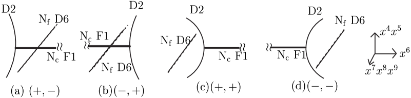
Figure 1: The rough sketch for the configuration according to the combinations of (sign$\{\pm 2{\rm N}_{\rm c}\}$,sign$\{\phi_{0}\}$)

3.2 Fundamental String Charge and Eleventh Dimension

It is well known that the electric charge on the D-brane corresponds to the fundamental string charge. In this section, we will discuss the relation between the two kinds of charge in our model to connect the gauge field to the eleventh dimension. First, we can rewrite the Gauss-Law (13) as

$$\vec{\nabla}_{u}\left\{{\rm H}\vec{\nabla}_{u}a+{\rm N}_{\rm f}\left(\frac{\Lambda\phi}{R}-{\rm sign}(\phi_{0})\right)\frac{{\vec{u}}}{|u|^{2}}\right\}=\pm 4\pi{\rm N}_{\rm c}\delta(u^{4})\delta(u^{5}).$$ (21)

Remember that from the action (12), the electric charge ${\rm Q_{E}}$ is given by the integral of the left hand side as

$${\rm Q_{E}}=\frac{1}{4\pi}\oint*\left\{{\rm H}\vec{\nabla}_{u}a+{\rm N}_{\rm f}\left(\frac{\Lambda\phi}{R}-{\rm sign}(\phi_{0})\right)\frac{{\vec{u}}}{|u|^{2}}\right\}=\pm{\rm N}_{\rm c},$$ (22)

where $*$ means the dual in the 2D space and this integral is calculated over the circle at the fixed $|u|$. The right hand side of this equation indicates that only the explicit external $\pm{\rm N}_{\rm c}$ F1 source is the total electric charge. This is the consistent with the fact that in our model, there is only $\pm{\rm N}_{\rm c}$ F1 source from the starting point. But what is the meaning of the left hand side ? The second term is the Witten effect coming from the Chern-Simons term. The above result shows that this term gives the additional induced charge, but is canceled by the nontrivial contribution from ${\rm H}\vec{\nabla}_{u}a$. In order to give this additional contribution, the gauge field $a$ turns out to show the nontrivial behavior. This makes $\phi$ nontrivial because $a$ and $\phi$ are related by supersymmetry (’almost’ BPS condition). This is the dielectric effect and the similar effect to Myer’s effect [36] which happens in another supersymmetric configuration like D6(123789)-D2(89) system. The definition of the electric current is different according to the sign of $\phi_{0}$. This difference produces the interpretation of the string creation or Hanany-Witten effect. Note that the observer on the D2-brane never sees such string creation because there is only external $\pm{\rm N}_{\rm c}$ electric charge on the D2-brane. But this relative difference is important for the whole system and we need the definition of the current which is applicable for the whole system.

So let us take the current of $\phi_{0}>0$ as the standard. Then we define the ’dual’ field as

$$\tilde{\nabla}_{u}\chi\equiv{\rm H}\vec{\nabla}_{u}a+{\rm N}_{\rm f}\left(\frac{\Lambda\phi}{R}-1\right)\frac{{\vec{u}}}{|u|^{2}}\hskip 56.9055pt\tilde{\nabla}_{u}\equiv\left({-\partial_{5}^{u}}\atop{\partial_{4}^{u}}\right)$$ (23)

By this definition, we can change the dynamical variable from $(a,\phi)$ to $(\chi,\phi)$. This $\chi$ can measure the difference of the electric charge, namely the fundamental string charge. This means that $\chi$ can also measure the distance of the $x^{10}$ direction and that we can identify this $\chi$ as that appeared in section 2.

The classical solution for $\chi$ can be obtained from its definition and the Gauss-Low as

$$\chi=\Big{[}\mp 2{\rm N}_{\rm c}+{\rm N}_{\rm f}\left\{1-{\rm sign}(\phi_{0})\right\}\Big{]}\varphi+{\rm const.}\hskip 14.22636pt,$$ (24)

where we define $\varphi$ by $u=u^{4}+iu^{5}=|u|{\rm e}^{i\varphi}$. By combining this solution with that of $\phi$, we obtain the solution expressed in the complex ’coordinate’ $y$ appeared in section 2 as

$$\ln y = \frac{{\tilde{\phi}}+i\chi}{2}=\frac{1}{2}\left\{\phi+i\chi+{\rm N}_{\rm f}\ln\left(\frac{R+\Lambda\phi}{\Lambda}\right)\right\}$$ (25)

$$= \mp{\rm N}_{\rm c}\ln\left(\frac{u}{\Lambda}\right)+\frac{{\rm N}_{\rm f}}{2}\left\{1-{\rm sign}(\phi_{0})\right\}\ln\left(\frac{u}{\Lambda}\right)+{\rm const.}$$

In addition to $y$, let us define another complex variable $w$,

$$w\equiv{\rm e}^{-(\phi+i\chi)/2}\left(\frac{u}{|u|}\right)^{{\rm N}_{\rm f}}\left(\frac{-\phi\Lambda+R}{\Lambda}\right)^{{\rm N}_{\rm f}/2}.$$ (26)

Then we can express the above solution by using these complex variables as

$$y = \left(\frac{u}{\Lambda}\right)^{\mp{\rm N}_{\rm c}}\times{\rm const.}\hskip 85.35826pt\phi_{0}>0$$

$$w = \left(\frac{u}{\Lambda}\right)^{\pm{\rm N}_{\rm c}}\times{\rm const.}\hskip 85.35826pt\phi_{0}<0.$$

This expresses the holomorphic embedding in the four dimensional space with $A_{{\rm N}_{\rm f}-1}$ singularity, $yw=(u/\Lambda)^{N_{f}}$. This is the expected result from the analysis when we lift our model to M-theory and study the supersymmetric cycle of the M2-brane on the multi Taub-NUT background with coincident ${\rm N}_{\rm f}$ monopoles.

Note that until now, we have considered the case in which the external ${\rm N}_{\rm c}$ strings have infinite length. This means that the source with the ${\rm N}_{\rm c}$ charges is too heavy to have the dynamics. This is why our analysis in Type IIA theory agrees with that of M-theory. If these strings are not infinite, that is, the source is not so heavy, there will be some dynamical effect as it happens in the case of MQCD. Therefore the analysis in Type IIA theory is limited within the approximation in which we can ignore this effect.

3.3 Two D2-branes with Heavy Quarks on D6 Background

Let us generalize the previous result to the case with two D2-branes and ${\rm N}_{\rm c}$ fundamental strings stretching between them. We consider the configuration in which the ${\rm N}_{\rm f}$ background D6-branes are located between the two D2-branes. This is the similar situation to the MQCD configuration. We can see that U(1)_-$\times$U(1)₊ gauge theory with heavy ${\rm N}_{\rm c}$ bifundamental quarks on the ${\rm N}_{\rm f}$ D6 background is realized on this configuration. Here, we distinguish each D2-brane and U(1) factor by $\pm$. This corresponds to the situation that the U(2) gauge theory is broken into the U(1)${}_{-}\times$U(1)₊ gauge theory by the relative difference between the nontrivial fields ${\tilde{\phi}_{\pm}}$ on the D2-branes. Then, we treat the two D2-branes almost independently except that in this situation, the signs of $\pm 2{\rm N}_{\rm c}$ and sign$(\phi_{0}){\rm N}_{\rm f}$ appear in the combination as $(-2{\rm N}_{\rm c},{\rm N}_{\rm f})$ and $(+2{\rm N}_{\rm c},-{\rm N}_{\rm f})$. (see Fig.1 and Fig.2.)

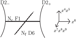
Figure 2: The combination of (a) and (b) of Fig.1.

This leads to that the relative distance $\Delta\{\ln y\}\equiv(\ln y_{+}-\ln y_{-})$ is determined as

$$\Delta\{\ln y\}=\ln y_{+}-\ln y_{-}=\frac{1}{2}\left\{\Delta{\rm\tilde{\phi}}+i\Delta\chi\right\}=(2{\rm N}_{\rm c}-{\rm N}_{\rm f})\ln\frac{u}{\Lambda}+{\rm const.}\hskip 28.45274pt.$$ (27)

This is the correct behavior for the RG-flow of SU(${\rm N}_{\rm c}$) SQCD with ${\rm N}_{\rm f}$ flavors.

4 T-dualized Configuration

Until now, we have discussed the configuration which is analogous to the MQCD configuration. We have studied the $2+1$ dimensional field theory realized on this configuration. In this section, we discuss the T-dualized configuration in the direction of $x^{6}$. For our original purpose, we have to realize the equivalent $2+1$ dimensional field theory also on the T-dualized configuration. What does the previous D2-D6 system transform under the T-duality ? Naively it seems to be D3-branes on the background of the D7 SUGRA solution. But, there might be some confusion about what is the background after the T-duality.

In the previous attempts [16][17], they have considered the Type IIB configuration with the orbifold on the D7 SUGRA background. They have regarded this configuration as the T-dual of the MQCD configuration with two NS5-branes on the D6 SUGRA background. As a result of that, the logarithmic behavior of the D7 SUGRA solution makes the analysis very messy. This also hampers having the AdS₅ structure in the conformal case, as found in [16]. This logarithmic behavior is the origin of the abnormal (complicated) behavior of their result. This strongly suggests that the D7 SUGRA background will not be the correct background as the T-dual of the MQCD configuration.

The most important point is that the region where the D7 classical solution is effective corresponds to that of the MQCD configuration with the small $x^{6}$-radius. In this region, the two NS5-branes are wrapping this direction and crossing each other. We can not expect that the ordinary 4D gauge theory is realized on this configuration. So it is unlikely that the role of the D6 SUGRA solution as the background will simply be succeeded to the D7 SUGRA solution.

In other words, the background in Type IIB theory must have the radius $R^{{\rm IIB}}$ which satisfies the relation $R_{6}^{\rm IIA}=\alpha^{\prime}/R_{6}^{\rm IIB}\rightarrow\infty$. This is the situation for the D6 background in the MQCD configuration. In this sense, the D7 SUGRA solution is not equivalent to the D6 SUGRA background in the MQCD configuration. The D7-brane solution is obtained from the small $R^{{\rm IIA}}$ limit of the D6 solution. On the other hand, this requirement is satisfied in the case of pure SYM theory; the backgrounds are flat before and after the T-duality.

Also in our simplified model (T-dual of the D2-D6 system), the D7 SUGRA background will not be the correct background. But it is very plausible that the scalar field $X^{6}/2\pi\alpha^{\prime}$ on the D2-brane world volume is transformed into the Wilson line (or gauge field) $A_{6}$ on the D3-brane. Then, the form of the D3-brane action after such translation enables us to guess at least how is the background which interacts with the fields on the D3-brane.

Let us look back at the D2-brane action (12) and consider how the action will change after the plausible T-duality. After rewriting ($\phi$, $a$) by ($a_{6}$, $a_{0}$), where $a_{6}\equiv\frac{A_{6}}{\Lambda}$ and $a_{0}\equiv\frac{A_{0}}{\Lambda}$, we expect that the D2-brane action reduces to that of the D3-brane with the delocalized direction of $x^{6}$. The D3-brane action after the dimensional reduction in this direction will be

$$S_{{\rm D3}} = -\frac{\Lambda}{4\pi}\int dtdu^{4}du^{5}{\rm H}\Bigg{[}\frac{1}{\Lambda^{2}}+\frac{1}{2}\Big{|}\vec{\nabla}_{u}a_{6}\Big{|}^{2}-\frac{1}{2}\left|\vec{\nabla}_{u}a_{0}\right|^{2}+O(\Lambda^{2})\Bigg{]}$$ (28)

$$\hskip 56.9055pt+\frac{\Lambda^{2}}{4\pi}\int dtdu^{4}du^{5}\frac{{\rm N}_{\rm f}}{R^{2}}\left(\frac{a_{6}}{R}-\vec{\nabla}_{u}a_{6}\cdot\frac{\vec{u}}{R}\right)a_{0},$$

where we define $R$ and H as $R\equiv\sqrt{|u|^{2}+\left(\Lambda a_{6}\right)^{2}}$ and ${\rm H}\equiv 1+\frac{\Lambda{\rm N}_{\rm f}}{R}$.

Let us estimate the form of the ’background’ on the D3-brane which gives the D3-brane action (28). It is known that the D3 brane action on the general background can be written as,

$$S_{{\rm D3}}=-T_{{\rm D3}}\int d^{4}\sigma{\rm e}^{-\phi}\sqrt{-{\rm det}\left(g_{MN}\partial_{\alpha}X^{M}\partial_{\beta}X^{N}+2\pi\alpha^{\prime}F_{\alpha\beta}\right)}+\frac{1}{4\pi^{2}g_{s}\alpha^{\prime}}\int G^{{\rm R}}_{(3)}\wedge A_{(1)},$$

$$\hskip 71.13188ptG^{{\rm R}}_{(3)}\equiv dB^{\rm R}_{(2)}+\left(B^{{\rm NS}}_{(2)}+{2\pi\alpha^{\prime}F}_{(2)}\right)\wedge dC^{\rm R}_{(0)},$$ (29)

where we defined $T_{{\rm D3}}$ as the D3-brane tension $T_{{\rm{D3}}}=(8\pi^{3}g_{s}{\alpha^{\prime}}^{2})^{-1}$. In the above equation, $B^{\rm R}_{(2)},B^{{\rm NS}}_{(2)}$ and $C^{\rm R}_{(0)}$ are the RR 2-form, NSNS 2-form and RR 0-form gauge field respectively. First, we have to careful of the region where the field theory is the good description. Let us denote the radius in the direction of $x^{6}$ in Type IIB theory as $R_{6}$ (=$R_{6}^{{\rm IIB}}$) for simplicity. By using the relation of the string coupling constant between before (IIA) and after (IIB) the T-duality, $g^{A}_{s}={g^{B}_{s}}{{\alpha^{\prime}}^{1/2}}/{R_{6}}$, we can express $\Lambda$ as $\Lambda={g^{A}_{s}}/\left(4\pi{\alpha^{\prime}}^{1/2}\right)={g^{B}_{s}}/\left(4\pi{R_{6}}\right)$. Then in Type IIB theory, we can take the similar limit to (6) as

$$g_{s}\rightarrow 0\ \ ,\hskip 17.07182ptR_{6}\rightarrow 0\ \ ,\hskip 28.45274pt z\rightarrow 0\ \ ,\hskip 17.07182pt\alpha^{\prime}\rightarrow 0\ \ ,$$

$$\Lambda\equiv\frac{g_{s}}{4\pi R_{6}}\ \ ,\hskip 8.5359pt u\equiv\frac{z}{2\pi\alpha^{\prime}}\hskip 14.22636pt{\rm fixed}\ \ .$$ (30)

In addition to the above limit, let us take the limit $\alpha^{\prime}/R_{6}\rightarrow\infty$. This means that the compactified radius of $x^{6}$-direction becomes infinite in Type IIA theory. This is the same situation as that in the previous sections.

Then we can easily read off the ’background’ from the actions (28) and (29) in the limit of (30). The ’background’ is written as

$$ds_{10}^{2}={\rm H}^{-\frac{1}{2}}\left\{\eta_{\mu\nu}dx^{\mu}dx^{\nu}+\sum_{i=7,8,9}(dx^{i})^{2}+(dx^{6})^{2}\right\}+{\rm H}^{\frac{1}{2}}|dz|^{2},$$

$${\rm e}^{-\phi}={\rm g}_{\rm s}^{-1}{\rm H},$$ (31)

$$\partial_{4}B^{\rm R}_{56}-\partial_{5}B^{\rm R}_{46}=\frac{{\rm N}_{\rm f}a_{6}\Lambda^{2}}{2\pi\alpha^{\prime}R^{3}},\hskip 28.45274pt\vec{\nabla}C^{\rm R}_{(0)}=\frac{{\rm N}_{\rm f}\Lambda}{2\pi\alpha^{\prime}R^{3}}\left({-u^{5}}\atop{u^{4}}\right),\hskip 28.45274ptB^{\rm NS}_{64}=B^{\rm NS}_{56}=0,$$

where we take the static gauge for the action (29) as before. Here we define $\vec{\nabla}$ as the derivative with respect to the original coordinates of the 2D space $(x^{4},x^{5})$. Note that in the above expression, the above ’background’ expresses the only gravitational field on the D3-brane. We can not guess how the background behaves in the bulk away from the D3-brane. But we have to remember that only the geometry near the brane is important for the AdS/CFT correspondence. So it is enough for that purpose to obtain the information about the background on the brane.

Note that the inclusion of the Wilson line with periodicity means that this expression contains all the winding modes of the $x^{6}$-direction. This is equivalent to the fact that the D6-supergravity background contains all the Kaluza-Klein (KK) modes in this direction. As the radius $R_{6}$ becomes large, the effect of the non-zero winding modes drops and we have to change the warped factor as

$$\frac{\Lambda{\rm N}_{\rm f}}{R}\rightarrow\sum_{n=-\infty}^{\infty}\frac{\Lambda{\rm N}_{\rm f}}{\sqrt{|u|^{2}+(\Lambda a_{6}+n/R_{6})^{2}}}\ \ \stackrel{{\scriptstyle|u|\gg 1/R_{6}}}{{\mbox{\LARGE{$\sim$}}}}\ \ \frac{g_{s}{\rm N}_{\rm f}}{2\pi}\ln|u|+{\rm const.}\hskip 28.45274pt.$$ (32)

Then the above ’background’ becomes the simple D7 supergravity solution with the non-trivial dilaton and RR 0-form. It is this simple D7 solution that has been used in [16][17] as the background. But in the region with the large radius $R_{6}$ (small radius $\alpha^{\prime}/R_{6}$ in Type IIA), we can not expect any more that the result of the MQCD analysis will be reproduced in Type IIB theory. This will be the reason why their result seems to be different from the result expected from the 4D field theory.

Here, we have to comment on the anomaly inflow mechanism [34] in the D3-D7 system with the two-dimensional intersection. This means the cancellation between the anomaly coming from the chiral fermion on the intersection and the anomaly from the bulk Chern-Simons term. In our model, the fermion one-loop effect is included in the first term of Eq.(29) and the bulk Chern-Simons term corresponds to the second term. As for the first term, this is the picture of the closed string. These two contributions are canceled under the BPS condition such as $\vec{\nabla}a_{0}=-\vec{\nabla}a_{6}$ and the Gauss-Low.

Next, let us discuss the behavior of the field on this D3-brane. We can repeat the same procedure as before by replacing $(\phi,a)$ and $\phi_{0}$ in section 3 with $(a_{6},a_{0})$ and $\left.a_{6}\right|_{u=0}$. In the same way, we define the field which expresses the F1 density on the D3-brane as

$$\tilde{\nabla}_{u}\chi\equiv{\rm H}\vec{\nabla}_{u}a_{0}+{\rm N}_{\rm f}\left(\frac{\Lambda a_{6}}{R}-1\right)\frac{{\vec{u}}}{|u|^{2}}\hskip 85.35826pt\tilde{\nabla}_{u}\equiv\left({-\partial_{5}^{u}}\atop{\partial_{4}^{u}}\right).$$ (33)

What is the fundamental string like whose charge is described by the above field $\chi$ ? Let us consider the case with two D3-branes and $\pm{\rm N}_{\rm c}$ additional electric (F1) source on the flat background (${\rm N}_{\rm f}=0$). This also expresses the U(1)_-$\times$U(1)₊ gauge theory with ${\rm N}_{\rm c}$ bifundamental matters as discussed in the previous sections. The source is realized as the T-dual of the fundamental string in the previous section. This fundamental string in Type IIB theory is stretching over the vanishing distance between the two D3-branes, say, the distance in the direction $x^{i}$ $(i=7,8,9)$. As an example, the rough sketch is depicted as Fig.3. On the other hand, the information about the distance between the D2-brane is transferred to the integral on the vanishing 2-cycle $\Sigma(6i)$ of the NSNS 2-form field $\int_{\Sigma(6i)}B_{(6i)}^{{\rm NS}}$. This integral is also the holographic charge of the wave O_w per fundamental string mentioned in the above.

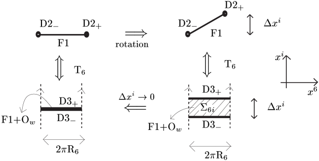
Figure 3: The sketch in the case of ${\rm N}_{\rm f}=0$. The number of the Type IIA fundamental strings transforms to that of the Type IIB fundamental strings. They are stretching over the the vanishing distance expressed as the zero limit of the small resolution $\Delta x^{i}$.

In the case with ${\rm N}_{\rm f}\neq 0$, there are also ${\rm N}_{\rm c}$ fundamental strings stretching over the vanishing distance. But different from the case with ${\rm N}_{\rm f}=0$, we have to generalize the NSNS 2-form field in the same way as $\Delta{\tilde{\phi}}$ in the previous section. This generalized NSNS 2-form field gives the correct wave O_w charge per fundamental string. These topics will be discussed in the following sections. Here we limit our analysis in this section within that of the world volume theory and proceed further.

Assuming that the bifundamental matters are too heavy to give dynamical effect, we can handle the two D3-branes almost independently. Then by using the similar complex coordinate $y$ to the previous sections,

$$\ln y\equiv\frac{{\tilde{a}_{6}}+i\chi}{2}=\frac{1}{2}\left\{a_{6}+i\chi+{\rm N}_{\rm f}\ln\left(\frac{R+\Lambda a_{6}}{\Lambda}\right)\right\},$$ (34)

we obtain the solutions and the difference between them as

$$\ln y_{\pm} = \pm\left\{{\rm N}_{\rm c}-\frac{{\rm N}_{\rm f}}{2}\right\}\ln\left(\frac{u}{\Lambda}\right)+\frac{{\rm N}_{\rm f}}{2}\ln\left(\frac{u}{\Lambda}\right)+{\rm const.}$$

$$\Delta\{\ln y\} = \ln y_{+}-\ln y_{-}=\frac{1}{2}\left(\Delta{\tilde{a}_{6}}+i\Delta\chi\right)=\left(2{\rm N}_{\rm c}-{\rm N}_{\rm f}\right)\ln\left(\frac{u}{\Lambda}\right)+{\rm const.}\hskip 14.22636pt.$$ (35)

5 From the Fields on the Brane to the Fields of Supergravity

In the previous section, we have learned that the (generalized) rescaled Wilson line $a_{6}$ (${\tilde{a}_{6}}$) and the new field $\chi$ on the D3-brane give the non-trivial solution due to the background in the action (28). Let us consider rewriting these non-trivial fields in terms of the Type IIB SUGRA matter (gauge) fields. This will be useful for the application to AdS/CFT (gravity/field theory) correspondence. This is also the necessary procedure because this teaches us how to transform these field under the sequence of T- and S-dualities.

What is the supergravity matter (gauge) fields corresponding to $a_{6}$ and $\chi$ ? First, let us consider the rescaled Wilson line $a_{6}$. It is well known that the Wilson line on one D-brane can be measured by the string world sheet coupled by NSNS 2-form field. This world sheet spans the circle of the compactified direction ($x^{6}$ direction in our case) and the orthogonal semi-infinite line from the point located by the D-brane. From the field theoretical point of view, a string stretching on this semi-infinite line expresses an external heavy quark on the D-brane. Then we can obtain the Wilson line by the integral of the gauge field over the (compactified) circle, that is, by the world sheet with NSNS 2-form field.

Let us discuss how to express the rescaled Wilson line $a_{6}$ in our model. First, let us consider $x^{i}$ as one of the coordinates $(x^{7},x^{8},x^{9})$. They are in the orthogonal directions to the D3-brane in the previous section. We have the relation between the NSNS field and the Wilson line as

$$\frac{1}{2\pi\alpha^{\prime}}\int_{0}^{2\pi{\rm R_{6}}}\int_{x^{i}=\infty}^{x^{i}=0}dx^{6}dx^{i}B_{6i}=\oint_{x^{i}=0}dx^{6}A_{6}-\oint_{x^{i}=\infty}dx^{6}A_{6},$$ (36)

where we denote $x^{i}=0$ as the position of the D3-brane in this direction. We set the Wilson line at infinity zero below. Remember that we consider the location of the ${\rm N}_{\rm f}$ D6-branes as the origin in the Type IIA analysis. This means the vanishing Wilson line for the background.

Then we have a relation between $a_{6}$ on the D3-brane and the NSNS field as

$$\frac{g_{s}a_{6}}{2}=\oint_{x^{i}=0}dx^{6}A_{6}=\frac{1}{2\pi\alpha^{\prime}}\int_{0}^{2\pi{\rm R_{6}}}\int_{x^{i}=\infty}^{x^{i}=0}dx^{6}dx^{i}B_{6i}^{{\rm NS}}.$$ (37)

Let us define new fields, $b^{{\rm NS}}$ and ${\tilde{b}^{{\rm NS}}}$ as the NS fields corresponding to $\left(g_{s}\Delta a_{6}\right)/{2}$ and $\left(g_{s}\Delta{\tilde{a}_{6}}\right)/{2}$ in the previous section. They can be written as

$$b^{{\rm NS}}\equiv\frac{1}{2\pi\alpha^{\prime}}\int_{\Sigma(6i)}B_{6i}^{{\rm NS}}dx^{6}dx^{i}=\oint A_{6}^{+}dx^{6}-\oint A_{6}^{-}dx^{6}=\frac{g_{s}}{2}\Delta a_{6},$$

$${\tilde{b}^{{\rm NS}}}\equiv\frac{1}{{2\pi\alpha^{\prime}}}\int_{\Sigma(6i)}{\tilde{B}_{6i}^{\rm NS}}dx^{6}dx^{i}\equiv\frac{g_{s}}{2}\Delta{\tilde{a}_{6}}=b^{{\rm NS}}+{\rm N}_{\rm f}\ln\left(\frac{{\rm R_{+}}+\Lambda a_{6+}}{{\rm R_{-}}+\Lambda a_{6-}}\right)$$

where $\frac{1}{2\pi\alpha^{\prime}}$ is the normalization factor for the 2-cycle $\Sigma(6i)$. As in the previous section, this 2-cycle spans the circle with the radius $R_{6}$ and the vanishing distance between the two D3-branes in the $x^{i}$ direction (see Fig.3). In the above, we distinguish the gauge field $A_{6}$, $a_{6}$ and R on each D3-brane by giving $+$ or $-$ on it. Note that as seen from these equations, $B_{6i}^{{\rm NS}}$ and ${\tilde{B}_{6i}}^{{\rm NS}}$ have only $x^{i}$ dependence as the delta function and has nontrivial $(x^{4},x^{5})$ dependence.

Next, let us discuss what is the supergravity fields corresponding to $\Delta\chi$. Remember that $\chi$ measures the difference of the string density on the D3-brane. As discussed in section 4, there are ${\rm N}_{\rm c}$ fundamental strings stretching over the vanishing distance between the two D3-branes in the direction of $x^{i}$ ($i=7,8,9$). Then we can see that the NSNS 2-form related to the F1 charge will be the correspondent to $\Delta\chi$. From the equation which gives the F1 charge on $(x^{4},x^{5})$ space, we get

$$\frac{1}{4\pi}\partial_{\alpha}\left(\Delta\chi\right)=\frac{1}{(4\pi^{2}\alpha^{\prime})^{3}}\int\left(*H_{(3)}^{{\rm NS}}{\rm e}^{-\phi}\right)_{\alpha 1236jk}dx^{123}dx^{6}dx^{jk}=\frac{1}{(4\pi^{2}\alpha^{\prime})^{3}}\int H^{{\rm NS}}_{\alpha 1236jk}dx^{123}dx^{6}dx^{jk},$$

where the indices $\{j,k\}$ are in $\{7,8,9\}$, but $\{j,k\}\neq i$, and the index $\alpha$ is in $\{4,5\}$. In the above, $\frac{1}{({4\pi^{2}\alpha^{\prime}})^{3}}$ is the normalization to give the integer F1 charge. We also use the last expression as the Poincare dual of the NS-NS 3-form field strength. In the T-dualized (Type IIB) model, the directions of $\{x^{0123},x^{6}\}$ are delocalized. So we can see that this 7-form $H^{{\rm NS}}_{\alpha 1236jk}$ has $(x^{j},x^{k})$ dependence as the delta function in addition to nontrivial $(x^{4},x^{5})$ dependence.

Then we can write down the solution in terms of the fields of supergravity as

$$\frac{1}{2}\left\{\Delta{\tilde{a}_{6}}+i\Delta\chi\right\}=\frac{1}{2\pi\alpha^{\prime}}\int_{\Sigma(6i)}g_{s}^{-1}{\tilde{B}_{6i}}^{{\rm NS}}dx^{6}dx^{i}+\frac{i}{(2\pi)^{5}{\alpha^{\prime}}^{3}}\int B^{{\rm NS}}_{1236jk}dx^{123}dx^{6}dx^{jk}$$

$$\hskip 56.9055pt=\left(2{\rm N}_{\rm c}-{\rm N}_{\rm f}\right)\ln u+{\rm const.}\hskip 14.22636pt,$$ (38)

where the NSNS 6-form gauge field $B^{{\rm NS}}_{1236jk}$ is defined as $\partial_{\alpha}B^{{\rm NS}}_{1236jk}=H^{{\rm NS}}_{\alpha 1236jk}$. Note that the above supergravity gauge fields are living only ’between’ the two overlapping D3-branes and similar to those of the twisted sector on the orbifold. But we have to be careful of the fact that the above real part is not written only by $\frac{1}{2\pi\alpha^{\prime}}\int_{\Sigma(6i)}{\rm e}^{-\phi}B_{6i}^{{\rm NS}}$, which is different from the case of pure SYM theory. Note that the integral $\frac{1}{2\pi\alpha^{\prime}}\int_{\Sigma(6i)}g_{s}^{-1}{\tilde{B}_{6i}}^{{\rm NS}}dx^{6}dx^{i}$ is also the holographic wave charge per fundamental string.

It will be interesting to bring our results to the configuration in which the four dimensional gauge theory is realized. This is the topic of the next section.

6 4D ${\cal N}$=2 Field Theory and Gravity Solution

6.1 Gauge Coupling Constant and 2-Form Fields

Let us take T-dualities and S-dualities of our configuration, and make the model in which 4D ${\cal N}$=2 SQCD is realized. This is the T-dualized model obtained from the well-known MQCD configuration mentioned in section 2 and our result will give us some knowledge of what it is like.

We consider the sequences of the dualities, ${\rm T_{36}ST_{12}ST_{36}}$, where the indices mean the directions of which we take T-dualities. Remember that the directions $\{x_{1},x_{2},x_{3}\}$ do not play any active role in our analysis. On the D2 world volume, the three scalar fields for these directions are free and decoupled from the remaining interacting action (12). In fact, we can easily confirm that there is no warped factor H on their kinetic terms. So we can safely delocalize these directions without changing our analysis. This is also the reason why the two-dimensional supersymmetric cycle for the M2-brane on the Taub-NUT background is the same as that of the M5-brane on the same background. As for the direction of $x_{6}$, we have already discussed the T-duality in this direction with special care in the section 4. The other directions $\{x_{4},x_{5},x_{7},x_{8},x_{9}\}$ are important for the structure of the vacua of the 4D field theory, but we do not take the T-dualities of these directions.

Let us consider what the constituents in our model will transform into. They are expected to transform under these dualities as

$$\frac{1}{2\pi\alpha^{\prime}}\int_{\Sigma(6i)}g_{s}^{-1}{\tilde{B}_{6i}^{{\rm NS}}}dx^{6}dx^{i}\hskip 28.45274pt \rightarrow \hskip 28.45274pt\frac{1}{2\pi\alpha^{\prime}}\int_{\Sigma(6i)}g_{s}^{-1}{\tilde{B}_{6i}^{{\rm NS}}}dx^{6}dx^{i}$$

$$\hskip 28.45274pt\frac{1}{(2\pi)^{5}{\alpha^{\prime}}^{3}}\int_{\Sigma(jk)}B^{{\rm NS}}_{1236jk}dx^{123}dx^{6}dx^{jk}\hskip 28.45274pt \rightarrow \hskip 28.45274pt\frac{1}{2\pi\alpha^{\prime}}\int_{\Sigma(jk)}B^{{\rm R}}_{jk}dx^{jk}$$

$$\hskip 28.45274pt{\rm D3}(456)\hskip 28.45274pt \rightarrow \hskip 28.45274pt{\rm Kaluza-Klein\ \ monopole}(12345)$$

$$\hskip 28.45274pt{\rm N_{c}\ \ F1}(i)\hskip 28.45274pt \rightarrow \hskip 28.45274pt{\rm N_{c}\ \ D5}(1236i)$$

$$\hskip 28.45274pt{\rm O}_{w}(6)\hskip 28.45274pt \rightarrow \hskip 28.45274pt{\rm D3}(123).$$ (39)

In the above, we can see how the new NSNS 2-form ${\tilde{B}_{6i}^{{\rm NS}}}$ transforms by Eq.(37) and the property $B^{{\rm NS}}_{6i}\rightarrow B^{{\rm NS}}_{6i}$ under this transformation. We also have to mention that the background does not change as seen from the explicit form (31). Note that the ${\rm N}_{\rm c}$ strings stretching over the vanishing distance between the two D3-branes transform into ${\rm N}_{\rm c}$ D5-branes (1236i), which are also wrapping the vanishing 2-cycle(6i) between the two Kaluza-Klein (KK) monopoles. In addition to that, because of the existence of NSNS 2-form ${\tilde{B}_{6i}^{{\rm NS}}}$, there is also induced D3-brane$(123)$ charge in the D5-brane in the same way as the wave in the previous section. Due to this induced charge, there is non-trivial RR 5-form flux. We also remark that the 4D gauge coupling constant corresponds to the field $\int_{\Sigma(6i)}g_{s}^{-1}{\tilde{B}_{6i}}^{{\rm NS}}dx^{6}dx^{i}$ and that this is not written only by $\int_{\Sigma(6i)}{\rm e}^{-\phi}B_{6i}^{{\rm NS}}dx^{6}dx^{i}$. By Eq.(38), we obtain the solutions for the above NSNS and RR 2-forms in the complex form as

$$-i\gamma\equiv\frac{1}{2\pi\alpha^{\prime}}\int_{\Sigma(6i)}g_{s}^{-1}{\tilde{B}_{6i}^{{\rm NS}}}dx^{6}dx^{i}+\frac{i}{2\pi\alpha^{\prime}}\int_{\Sigma(jk)}B^{{\rm R}}_{jk}dx^{jk}=\left(2{\rm N}_{\rm c}-{\rm N}_{\rm f}\right)\ln u+{\rm const.}\ \ \ .$$ (40)

This is the modified twisted sector of the 2-forms on the background.

6.2 Gravity Dual: Suggestion

Let us discuss the supergravity dual corresponding to this configuration. For this purpose, let us reconsider the MQCD configuration first. It consists of ${\rm N}_{\rm f}$ rigid D6-branes, and (NS5,D4)-branes. The state or shape of (NS5,D4)-branes is determined by the BPS condition on the ${\rm N}_{\rm f}$ D6 supergravity background. The important point is that the shape of these (NS5,D4)-branes has the information about the field theory dynamics. Therefore, in order to discuss the gravity dual, we have to extract or separate the gravity induced by these (NS5,D4)-branes from the background. This is very difficult task. But remember that the solution of the ${\rm N}_{\rm f}$ D6 SUGRA solution becomes ${\rm N}_{\rm f}$ KK monopole solution in the eleven-dimensional supergravity. Moreover, after the large ${\rm N}_{\rm f}$ limit, this reduces to ${\rm Z}_{{\rm N}_{\rm f}}$ orbifold, that is, locally flat metric [37][38]. This simplifies the problem, and it will be possible to carry out the above extraction. In general, the locally flat metric transforms another locally flat metric under the T-duality. So the above observation indicates that also in Type IIB configuration, there is such a frame in which the background becomes locally flat.

In addition to that, we have to remember that it is only the relative (generalized) distance $\Delta{\tilde{x}^{6}}$ between the two NS5-branes that has the physical meaning as the RG flow of the (complex) gauge coupling constant. The position itself in the direction of ${\tilde{x}^{6}}$ does not effect on the 4D field theory. This means that there is one extra degree of freedom for the 4D field theory. This enables us to delocalize the configuration in this direction, keeping the relative distance fixed. This also simplified the problem.

As a conclusion, we can say that the problem will become easy in the following procedure:
(1) By adding the extra dimension, set the background to be the locally flat.
(2) On this background, delocalize the configuration in the irrelevant direction for the 4D       field theory.

But in Type IIB theory, the reliable higher dimensional effective theory is not known. This is the different point from Type IIA theory related to the eleven-dimensional supergravity. So our following analysis is based on only the analogy of Type IIA theory and the result is limited within the suggestion of the procedure to obtain the possible dual of the corresponding field theory.

Let us return to our model in Type IIB theory and consider the problem in the same spirit as the above. What is the appropriate parameter which should be promoted to the additional space coordinate ? The electric field (or the temporal component of the gauge field) on the D-brane will be the promising candidate. This is because this field is known to have the relation with the eleventh dimension in Type IIA, as discussed in the previous sections.

On the other hand, the coordinate $x^{6}$ in Type IIB theory does not play any active role. The configuration is delocalized in this direction and the role of the coordinate $x^{6}$ in the MQCD analysis is succeeded to the Wilson line. As a result of that, Type IIB theory we have been discussed is the almost nine-dimensional theory. So let us promote also the Wilson line to the new coordinate. Then this almost nine-dimensional theory is on the same level with the ten-dimensional Type IIA theory on the point of the degree of freedom for the space-time dimension.

We have to note that the two-dimensional space ($x^{6},x^{10}$) in M-theory is related by the T-duality to the torus with the complex structure $\tau\equiv C_{0}+i/g_{s}$ in Type IIB theory [26]. So we can expect that the electric field and the Wilson line play the role of the new coordinates of this additional two-dimensional space for Type IIB theory.

On the KK monopole, the Wilson line and the electric field correspond to the NSNS and RR 2-forms respectively as already seen in the sequence of the T- and S-dualities. These two parameters can be observed only on the branes in Type IIB theory. But, by including them as the new space coordinates, we can formally extend our discussion to twelve-dimensional space-time. Let us define the new coordinate as

$$x^{{\rm NS}}\equiv\frac{a_{6}g_{s}}{2},\hskip 56.9055ptx^{{\rm R}}\equiv\frac{\chi}{2}.$$ (41)

Note that $x^{{\rm R}}$ and $x^{{\rm NS}}$ are the periodic coordinates. But in our discussion, the Wilson line $x^{{\rm NS}}$ always appears in the form $d{\tilde{x}_{{\rm NS}}}\equiv{\rm e}^{-\phi}dx_{{\rm NS}}$ with the string coupling constant $g_{s}\rightarrow 0$. So the coordinate ${\tilde{x}_{{\rm NS}}}$ runs from $-\infty$ to $+\infty$ in the same way as $a_{6}$ or ${\tilde{a}_{6}}$. This also means that there is no S-invariance of the SL(2 Z) and S-transformation is fixed in our analysis.

How can we lift the ten-dimensional supergravity solution to the twelve-dimensional solutions ? The hint is given by the T-invariance of the SL(2 Z) and the analogy of the lift from Type IIA to eleven-dimensional supergravity. We suggest the form as

$$ds_{12}^{2} = {\rm e}^{-\phi/2}g_{s}^{1/2}ds_{10}^{2}+{\rm e}^{\phi}g_{s}^{-1}ds_{2}^{2}$$

$$ds_{2}^{2}\equiv\left(\frac{g_{s}\alpha^{\prime}}{R_{6}}\right)^{2}\left[{\rm e}^{-2\phi}dx_{{\rm NS}}^{2}+\left\{dx_{R}-dx^{M}\oint\left(B^{{\rm R}}_{6M}-C_{0}B^{{\rm NS}}_{6M}\right)\frac{dx^{6}}{2\pi\alpha^{\prime}}\right\}^{2}\right]$$

where $M$ means the indices for the ten dimensional space-time and runs from $0$ to $9$. The factor $\frac{g_{s}\alpha^{\prime}}{R_{6}}$ corresponds to the radius of the eleventh dimension in Type IIA theory. We can see that by the above warped factor of the dilaton, the Einstein action $\int\sqrt{-g^{(12)}}R^{(12)}$ in the twelve dimensions reduces to the ten-dimensional action in the string frame $\int\sqrt{-g^{(10)}}{\rm e}^{-2\phi}R^{(10)}$.

Note that the degrees of freedom for the metric are the same as eleven-dimensional supergravity. This is because the relative factor for $dx_{{\rm NS}}^{2}$ and $dx_{{\rm R}}^{2}$ is fixed by T-invariance and there is the constraint that all the fields (and metric) are independent of $x^{6}$ with the isometry. The latter reason comes from the requirement of the T-dual of Type IIA theory.

This is the important point. There is the well-known fact that there is no supergravity theory in the full twelve-dimensional space-time. But we have to note that the above expression is defined only under the above conditions. As a result of that, the above expression is essentially eleven-dimensional one. So the no-go theorem in the full twelve-dimensional space-time does not mean that supersymmetry does not exist in our model.

By this lift rule, the ’background’ Eq.(31) becomes the KK-monopole solution,

$$ds_{12}^{2}=\eta_{\mu\nu}dx^{\mu}dx^{\nu}+\sum_{i=7,8,9}(dx^{i})^{2}+(dx^{6})^{2}+ds_{4}^{2},$$ (43)

$$ds_{4}^{2}\equiv\left(2\pi\alpha^{\prime}\right)^{2}\left\{{\rm H}\left(|du|^{2}+\Lambda^{2}da_{6}^{2}\right)+{\rm H}^{-1}{\Lambda^{2}}\Big{[}d\chi+{\rm N}_{\rm f}\left(\frac{\Lambda a_{6}}{R}-1\right)d\varphi\Big{]}^{2}\right\},$$

where we use the same notation used in Eq.(24) and Eq.(31). Then, let us take the large ${\rm N}_{\rm f}$ limit along with the limit in the previous sections. By this limit, the warped factor H reduces as ${\rm H}=1+\Lambda{\rm N}_{\rm f}/R\rightarrow\Lambda{\rm N}_{\rm f}/R$. Then we obtain the locally flat metric as

$$ds_{12}^{2}=\eta_{\mu\nu}dx^{\mu}dx^{\nu}+\sum_{i=7,8,9}(dx^{i})^{2}+(dx^{6})^{2}+\left(2\pi\alpha^{\prime}\right)^{2}\left|d{\cal M}^{(4)}_{{\rm Z_{{\rm N}_{\rm f}}}}\right|^{2},$$

$$\hskip 42.67912pt\left|d{\cal M}^{(4)}_{{\rm Z_{{\rm N}_{\rm f}}}}\right|^{2}\equiv\left|dV_{1}\right|^{2}+\left|dV_{2}\right|^{2},$$

$$V_{1}\equiv\left(2{\rm N}_{\rm f}\right)^{1/2}\Lambda\left(a_{6}+\frac{R}{\Lambda}\right)^{1/2}{\rm e}^{i\chi/2{\rm N}_{\rm f}},\hskip 8.5359ptV_{2}\equiv\left(2{\rm N}_{\rm f}\right)^{1/2}u\left(a_{6}+\frac{R}{\Lambda}\right)^{-1/2}{\rm e}^{-i\chi/2{\rm N}_{\rm f}}.$$ (44)

Note that in our notation, $\chi$ has the period $4\pi$ and this leads to the $Z_{{\rm N}_{\rm f}}$ orbifold identification $(V_{1},V_{2})\sim({\rm e}^{2\pi i/{\rm N}_{\rm f}}V_{1},{\rm e}^{-2\pi i/{\rm N}_{\rm f}}V_{2})$. We can see the above complex coordinates $\{V_{1},V_{2}\}$ have relations with the holomorphic coordinates $\{y,w\}$ of the Taub-NUT space as

$$y\equiv{\rm e}^{\left(a+i\chi\right)/2}\left(a_{6}+\frac{R}{\Lambda}\right)^{{\rm N}_{\rm f}/2}\hskip 71.13188pt\stackrel{{\scriptstyle{\rm N}_{\rm f}\rightarrow\infty}}{{\sim}}\ \ \ \left(2{\rm N}_{\rm f}\right)^{-{\rm N}_{\rm f}/2}\left(\frac{V_{1}}{\Lambda}\right)^{{\rm N}_{\rm f}},$$

$$w\equiv{\rm e}^{-\left(a+i\chi\right)/2}\left(\frac{u}{\Lambda}\right)^{{\rm N}_{\rm f}}\left(a_{6}+\frac{R}{\Lambda}\right)^{-{\rm N}_{\rm f}/2}\ \ \ \ \ \stackrel{{\scriptstyle{\rm N}_{\rm f}\rightarrow\infty}}{{\sim}}\ \ \ \left(2{\rm N}_{\rm f}\right)^{-{\rm N}_{\rm f}/2}\left(\frac{V_{2}}{\Lambda}\right)^{{\rm N}_{\rm f}}.$$

Then, our problem reduces to the embedding of the three kinds of ’matter’ although they are originally undivided.

(1)the two KK monopoles

(2)the complex 2-form Eq.(40) which exists between them

(3)the D3-brane charge induced in the ${\rm N}_{\rm c}$ external D5-branes

Let us consider the contribution coming from each part and discuss how to construct the gravity dual. First, let us concentrate on the two KK monopoles. Note that in section 4, we can see that the sum for ${\tilde{a}_{6}}+i\chi$ on each D3-brane is also non-trivial. We can see from Eq.(34) and Eq.(35),

$$\ln y_{{\rm S}}\equiv\ln y_{+}+\ln y_{-}=\frac{1}{2}\left\{{\tilde{a}_{6+}}+{\tilde{a}_{6-}}+i\left(\chi_{+}+\chi_{-}\right)\right\}={\rm N}_{\rm f}\ln\left(\frac{u}{\Lambda}\right)+{\rm const.}\hskip 56.9055pt$$ (45)

After the large ${\rm N}_{\rm f}$ limit, we obtain the corresponding position of the whole of the two D3-branes as ${\rm N}_{\rm f}\ln V_{2}^{{\rm S}}$= constant. In the same way, after the sequence of the T- and S-dualities in the section 6.1, we can reach the same conclusion$-$ The whole of two KK monopoles are located at ${\rm N}_{\rm f}\ln V_{2}={\rm N}_{\rm f}\ln V_{2}^{{\rm S}}$ : constant. Of course, there remains the relative distance which corresponds to the complex 2-form Eq.(40). Let us leave the contribution from this 2-form for the next discussion and concentrate on the contribution from the two KK monopoles themselves.

Note that we can not distinguish the direction of the KK monopole world volume from the direction in which the KK monopole charge is delocalized or distributed. For example, there are two kinds of the Type IIA KK monopole from the point of M-theory. One has the world volume in the direction of the eleventh dimension and the other is delocalized in this direction. The former type is obtained by the dimensional reduction from the KK monopole in M-theory with respect to the eleventh dimension. We can obtain the latter type by taking the T-dualities from the Type IIA NS5-brane, for example, T₅₆ dualities from the Type IIA NS5-brane(12345). But, the both types of the Type IIA KK monopole are described by the same classical solution in M-theory.

This means that when we delocalize the whole of the two KK monopoles in the direction of ${\rm N}_{\rm f}\ln V_{2}$, we can obtain the ordinary Type IIB KK monopole solution which is non-trivial only in the directions $\{x^{6},x^{7},x^{8},x^{9}\}$ and has the KK monopole charge with respect to the compactified direction of $x^{6}$. In the region where $x^{i}\sim 0$ ($i=7,8,9$), it is known that the supergravity solution for the two overlapping KK monopoles reduce to the orbifold ${\rm R^{4}/Z_{2}}$ [37].

Note that on the space of $V_{2}=V_{2}^{{\rm S}}$: constant, $V_{1}$ is the same as $u$ from the definition (44). So we can interpret $u$ in (40) as $V_{1}$ on the plane, $V_{2}=V_{2}^{{\rm S}}$: constant.

Therefore, our problem reduces to the embedding of the remaining two kinds of ’matter’ into the locally flat background such as

$$ds_{12}^{2}=\left\{\eta_{\mu\nu}dx^{\mu}dx^{\nu}+\left(2\pi\alpha^{\prime}\right)^{2}\left|d{\cal M}^{(4)}_{{\rm Z_{2}}}\right|^{2}+\left(2\pi\alpha^{\prime}\right)^{2}\left|dV_{1}\right|^{2}\right\}+\left(2\pi\alpha^{\prime}\right)^{2}\left|dV_{2}\right|^{2}$$ (46)

where we use $\left|d{\cal M}^{(4)}_{{\rm Z_{2}}}\right|^{2}$ as the symbol which expresses the 4D locally flat space with the $Z_{2}$ orbifold identification. The two kinds of ’matter’ are given as

(1)the twisted sector on the ${\rm R^{4}/Z_{2}}$ orbifold fixed point

$$-i\gamma={\rm N}_{\rm f}\left(\ln V_{2}^{-}-\ln V_{2}^{+}\right)=(2{\rm N}_{\rm c}-{\rm N}_{\rm f})\ln V_{1}+{\rm const.}$$ (47)

(2)the D3-brane charge induced in the ${\rm N}_{\rm c}$ external D5-branes wrapping the vanishing
           two cycle on the orbifold

Note that all the fields becomes independent of $V_{2}$ after being delocalized in this direction. As a result of that, this extra two-dimensional space does not play an important role for the remaining ten-dimensional theory. So we can conclude that what we have done is to add the extra two-dimensional space (41) and to pick up the unimportant another two-dimensional space ($V_{2}$-space) from the twelve dimensional space-time. This is the procedure similar to the M-theory flip. In this remaining ten-dimensional space-time, the generalized twisted sector becomes the ordinary one.

On the other hand, in F-theory it is known that the extra two-dimensional space corresponds to the space for the dilaton and axion of Type IIB theory. In the context of F-theory, our procedure is the replacement of the two-dimensional space for the non-trivial dilaton and axion with another two-dimensional space for the constant dilaton and axion. That is, we take the frame of the (remaining) ten-dimensional in which the dilaton and axion are constant. Our suggestion is that this remaining ten-dimensional space-time would be the dual of the corresponding field theory.

We also have to comment on the fundamental region of the 4D $Z_{{\rm N}_{\rm f}}$ orbifolded space. The fundamental region can be taken as ${\bf C}\times{\bf C/Z}_{{\rm N}_{\rm f}}$. When we delocalize the configuration in the $V_{2}$-space, the region of this space is ${\bf C/Z}_{{\rm N}_{\rm f}}$ because it is in the form of ${\rm N}_{\rm f}\ln V_{2}$ coming from Eq.(45) that we delocalize the configuration. As a result of that, the $V_{1}$-space spans the whole complex plane. In other words, the $Z_{{\rm N}_{\rm f}}$ orbifold identification is invisible for the remaining ten-dimensional space-time.

Then we can see that the above configuration is the same as that of pure SYM theory except the values of the D5 and D3-charge. This is consistent with the fact that at one-loop level, the structure of pure SYM vacua is qualitatively the same as the Coulomb branch of SQCD.

The ten-dimensional solution can be obtained by modifying the result for pure SYM [3]. They have discussed the supergravity solution for the N D5-branes wrapping on the vanishing two-cycle on the fixed point of the ${\rm R^{4}/Z_{2}}$ orbifold. But with only a bit of change about the D-brane charge, we can formally generalize their result.

The result is summarized as follows:

$$\hskip 14.22636ptds^{2}_{12}=ds^{2}_{10}+\left(2\pi\alpha^{\prime}\right)^{2}\left|dV_{2}\right|^{2}$$ (48)

$$\hskip 28.45274pt\left({2\pi\alpha^{\prime}}\right)^{-1}ds^{2}_{10}=\frac{\rho^{2}}{f(|V_{1}|,v)^{1/2}}\left\{\eta_{\mu\nu}dx^{\mu}dx^{\nu}\right\}+\frac{f(|V_{1}|,v)^{1/2}}{\rho^{2}}\left\{|dV_{1}|^{2}+d{\cal M}_{{\rm Z_{2}}}^{2}\right\},$$

$${f(|V_{1}|,v)}=8\pi g_{s}{\rm Q_{D3}}+2\left(2\pi g_{s}{\rm Q_{D5}}\right)^{2}\left[\ln\left\{\frac{\rho^{4}}{v^{2}}\right\}+\frac{|V_{1}|^{2}}{v^{2}}+{\rm const.}\right],$$

$$\hskip 113.81102pt\rho^{2}\equiv|V_{1}|^{2}+v^{2},\hskip 28.45274ptv\equiv\frac{R_{6}^{1/2}}{\alpha^{\prime}\pi}\left(\sum_{i=7,8,9}{x^{i}}^{2}\right)^{1/4},$$

$$\hskip 14.22636ptC_{(4)}=\rho^{4}{f(|V_{1}|,v)}^{-1}dx^{0}\wedge dx^{1}\wedge dx^{2}\wedge dx^{3},\hskip 28.45274ptB^{{\rm R}}_{(2)}=b^{{\rm R}}\omega_{(2)},\hskip 14.22636pt{\tilde{B}^{{\rm NS}}_{(2)}}={\tilde{b}^{{\rm NS}}}\omega_{(2)},$$

$$\hskip 56.9055pt\gamma\equiv\tau{\tilde{b}^{{\rm NS}}}-b^{{\rm R}}=iQ_{{\rm D5}}\ln V_{1}+{\rm const.}\hskip 28.45274pt\tau=\frac{i}{g_{s}}+C_{0}\ \ {\rm:}\ \ \ {\rm const.}\hskip 28.45274pt,$$

where we denote D3 and D5 charges as ${\rm Q_{D3}}$ and $Q_{{\rm D5}}$. In their case of pure SU(${\rm N}_{\rm c}$) SYM, the D5 charge is $Q_{{\rm D5}}=2{\rm N}_{\rm c}$, and for the D3 charge they have suggested $Q_{{\rm D3}}={\rm N}_{\rm c}/2$. We have replaced the original coordinate $u$ with $V_{1}$ as explained. In the above equation, we denote the 2-form which is dual to the vanishing 2-cycle $\Sigma$ as $\omega_{(2)}$. We normalize this integral of the 2-form over $\Sigma$, as $\frac{1}{2\pi\alpha^{\prime}}\int_{\Sigma}\omega_{(2)}=1$. This 2-form also satisfies the anti-selfduality condition, $\omega_{(2)}=-*\omega_{(2)}$. The components of the above NSNS and RR 2-forms $\big{\{}{\tilde{B}_{(2)}^{\rm NS}},B_{(2)}^{\rm R}\big{\}}$ are essentially the same as ${\tilde{B}_{6i}^{\rm NS}}$ and $B_{jk}^{\rm R}$, that we have obtained by T- and S-dualities in (39). In the following discussion, we set the RR 0-form $C_{0}$ to be zero.

Then let us consider the supergravity solution for our configuration. It is easy to see that in our case, the D5 charge is $Q_{{\rm D5}}=2{\rm N}_{\rm c}-{\rm N}_{\rm f}$. What about $Q_{{\rm D3}}$ ? As we have commented before, this charge is determined by the NSNS 2-form field ${\tilde{B}_{6i}^{\rm NS}}$ on the ${\rm N}_{\rm c}$ D5-branes. We approximate this as

$$Q_{{\rm D3}}=\frac{{\rm N}_{\rm c}}{4\pi^{2}\alpha^{\prime}}\int_{\Sigma}\left.{\tilde{B}^{{\rm NS}}_{(2)}}\right|_{V_{1}=\epsilon}=\frac{{\rm N}_{\rm c}}{2\pi}\left.{\tilde{b}^{{\rm NS}}}\right|_{V_{1}=\epsilon},$$ (49)

where $\epsilon$ means the low energy cut-off of $V_{1}$ in order to avoid the region where ${\tilde{b}^{{\rm NS}}}$ vanishes. Note that our approximations in section 3 and 4 about the bifundamental matters are broken down in this region. This is because they are not heavy any more and become massless. This is the typical limit for the perturbative analysis. The nonperturbative effect will cure this kind of singularity. Then we can also expect that the above D3-charge is determined by the low energy effective coupling constants for the U(1)${}^{{\rm N}_{\rm c}-1}$ gauge theories coming from the broken SU(${\rm N}_{\rm c}$) gauge symmetry. We need the Seiberg-Witten curve to determine these coupling constants, but this is beyond our current analysis.

We also have to comment on the scale of the Higgs branch. In the directions of $\{x^{7},x^{8},x^{9}\}$, we need the same limit as that of the MQCD analysis such as

$$x^{i}\rightarrow 0\hskip 85.35826pt{\tilde{v}^{2}}\equiv\frac{1}{{\alpha^{\prime}}^{3/2}}\left(\sum_{i=7,8,9}{x^{i}}^{2}\right)^{1/2}\ \ \ {\rm fixed}.$$ (50)

This scale ${\tilde{v}}$ corresponds to the directions of the vacuum expectation values for the quarks in the fundamental representations, and does not depend on the string coupling constant. In fact, the Higgs branch is known to have no quantum correction. Compared with $v$, we can easily see that ${\tilde{v}}\gg v\sim 0$ in our model (see (30) and (50)). Then only $V_{1}$ dependence remains in Eq.(48) because ${\tilde{v}}$ dependence never appears in this solution. Especially $\rho$ is determined by only $V_{1}$ and the holographic energy scale is expected to be $V_{1}$. These facts show that the above result corresponds to the Coulomb branch, not Higgs branch.

Note that the complex field $\gamma\equiv\tau{\tilde{b}^{{\rm NS}}}-b^{{\rm R}}$ corresponds to the complex gauge coupling constant of the gauge theory. This theory is realized on the ${\rm N}_{\rm c}$ D5-branes wrapping on the vanishing 2-cycle. In our analysis, the NSNS 2-form is generalized as compared with the ordinary one on the flat background (pure SYM), but reproduces the correct behavior of the gauge coupling constant for SQCD.

In [16] [17], it is suggested that this typical ratio 1/2 between ${\rm N}_{\rm c}$ and ${\rm N}_{\rm f}$ originates from the constant $b^{{\rm NS}}/2\pi=1/2$ on the orbifold. This is an interesting suggestion, but it seems to be different from our result about the RG flow. Our result is independent of this value. Moreover, in their model, this typical value of the NSNS 2-form field induces the D5-brane charge in the world volume of the ${\rm N}_{\rm f}$ D7-branes. In our model, the induced D5 charge is expected to come from the two Kaluza-Klein monopoles. These differences might be explained in terms of the Type IIA counterpart of the configuration; their configuration is the one in which D6-branes would be dynamical as D4 and NS5-branes rather than background.

It is important to comment on the case of ${\rm N}_{\rm f}=2{\rm N}_{\rm c}$. In this case, the D5 charge vanishes, and ${\tilde{b}^{{\rm NS}}}$ is the constant, which leads to the gauge coupling constant determined by the constant ${\tilde{b}^{{\rm NS}}}/g_{s}$. The solution reduces to

$$\hskip 14.22636ptds^{2}_{12}=ds^{2}_{10}+\left(2\pi\alpha^{\prime}\right)^{2}\left|dV_{2}\right|^{2}$$

$$\hskip 28.45274pt\left({2\pi\alpha^{\prime}}\right)^{-1}ds^{2}_{10}=\frac{\rho^{2}}{(4g_{s}{\rm N}_{\rm c}{\tilde{b}^{{\rm NS}}})^{1/2}}\left\{\eta_{\mu\nu}dx^{\mu}dx^{\nu}\right\}+\frac{(4g_{s}{\rm N}_{\rm c}{\tilde{b}^{{\rm NS}}})^{1/2}}{\rho^{2}}\left\{|dV_{1}|^{2}+d{\cal M}_{{\rm R^{4}/Z_{2}}}^{2}\right\},$$

$$\hskip 28.45274ptC_{(4)}=\frac{\rho^{4}}{4g_{s}{\rm N}_{\rm c}{\tilde{b}^{{\rm NS}}}}dx^{0}\wedge dx^{1}\wedge dx^{2}\wedge dx^{3}.\hskip 28.45274pt$$

We have to be careful of the region where the description of the supergravity will be correct. We keep the ratio $1/g_{YM}^{2}={\tilde{b}^{{\rm NS}}}/g_{s}$ fixed with $g_{s}\rightarrow 0$ and ${\tilde{b}^{{\rm NS}}}\rightarrow 0$. In addition to that, we also have to consider the region,

$$g_{s}{\rm Q_{D3}}=\frac{g_{s}{\rm N}_{\rm c}}{2\pi}{\tilde{b}^{{\rm NS}}}\gg 1.$$ (51)

This means that we need the large ${\rm N}_{\rm c}$ limit in the same way as the other known SUGRA solutions.

Note that except for $\rho\sim|V_{1}|$ in our case, the above solution is similar to that of [23]. But, our expression of the D3-brane charge has ${\tilde{b}^{{\rm NS}}}$ dependence, but theirs does not. The physical meaning of this difference can be explained as the following. Their configuration consists of ${\rm N}_{\rm c}$ D5-branes with $({{\rm N}_{\rm c}}b^{{\rm NS}})/{2\pi}$ D3-brane charge and ${\rm N}_{\rm c}$ anti-D5-branes with $\left(2\pi-b^{{\rm NS}}\right){{\rm N}_{\rm c}}/{2\pi}$ D3-brane charge. As a result of that, the total D3-brane charge is ${\rm N}_{\rm c}$ with vanishing D5 charge. The dependence on $b^{{\rm NS}}$ is gone. We can understand this difference more clearly in the MQCD configuration as depicted in Fig.4 In their case, the ${\rm N}_{\rm c}$ D4-branes are wrapping on the circle completely, but in our case they are wrapping on only a part of the circle.

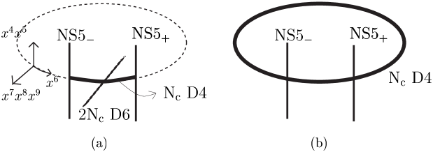
Figure 4: Two conformal configurations: (a) partially wrapping ${\rm N}_{\rm c}$ D4-branes (b) completely wrapping ${\rm N}_{\rm c}$ D4-branes

7 Speculations on the Nonperturbative Effect

In the previous sections, we have studied in the region where we can ignore the strong coupling effect $-$ nonperturbative effect. Let us consider what will happen beyond this perturbative region. Of course, we can not extend our analysis to this region, so we have to limit our discussion within speculation, but this kind of speculation will be useful.

For example, let us remember MQCD suggested by [18]. This is well known to be the most successful example in taking in the nonperturbative effect. The success of MQCD is based on the fact that in this model the D0-brane is responsible for the nonperturbative effect (instanton effect) of the 4D ${\cal N}$=2 SQCD. So lifting the whole system to the eleven dimensional supergravity gives the way to take in this effect. Note that in the system in which D0-brane does not play this key role, lifting to the 11D SUGRA does not solve the problem automatically.

Imagine that we did not know the fact that 11D SUGRA includes all the effects of the D0-brane in Type IIA theory. As long as we know that the D0-brane is responsible for the 4D instanton effect, we could say at least the followings; if all the effects of the D0-brane are included, D4-brane and NS5-brane would become the same thing. This expectation comes from the property of the 4D field theory that the nonperturbative effect makes the gauge coupling constant invisible after the dimensional transmutation. Moreover, from the knowledge of the purely field theoretical analysis, we can tell what this configuration would be like $-$ the configuration described by the Seiberg-Witten curve.

As seen in this case, the knowledge about well-known results of the field theory may enable us to give some clues about the unknown aspects of the string theory.

So let us speculate what will happen in the model that we have discussed. What is responsible for the nonperturbative effect in Type IIB theory ? By the T-duality of the D0-branes in the MQCD configuration, we can easily find out that it is the D1-branes that play that role. These D1-branes are wrapping on the vanishing 2-cycle on the orbifold. This is also confirmed by the analysis of the action [40] as done in [41] [42] for MQCD configuration. So it is plausible that the nonperturbative effect would be included if we could add all the D1-brane effects to the previous result. But it is technically very difficult to carry out such a task directly. So we have to limit our discussion within qualitative speculations about the configuration which would be described by the Seiberg-Witten curve. But this can be done without using the explicit (direct) calculations of the D1-brane effects.

First, let us consider simple pure SYM theory. In the weak coupling region, this is the Type IIB configuration discussed in [2][3] that is also the case of ${\rm N}_{\rm f}=0$ in our model. In this region, the flow of the gauge coupling constant is described as the complex field $\gamma\equiv\tau b^{{\rm NS}}-b^{{\rm R}}$.

From the success of MQCD, we know how this complex field behaves. Because this field corresponds to the distance between the two NS5-branes on the two-dimensional space $(x^{6},x^{10})$ in Type IIA theory, we can get the exact behavior of this complex field from the Seiberg-Witten curve as

$$\gamma\left(u\right)=i(\ln y_{+}-\ln y_{-}),\hskip 28.45274pty_{\pm}\equiv\sum_{n=0}^{{\rm N}_{\rm c}}s_{n}u^{n}\pm\sqrt{\left(\sum s_{n}u^{n}\right)^{2}-\Lambda_{{\rm QCD}}^{2{\rm N}_{\rm c}}}\ \ .$$ (52)

Here $\{s_{n}\}$ are the moduli parameters which satisfies the conditions, $s_{{\rm N}_{\rm c}}=1$ and $s_{{\rm N}_{\rm c}-1}=0$. We also denote the dynamical scale for this gauge theory as $\Lambda_{{\rm QCD}}$. The above $y_{\pm}$ are the solution of the quadratic equation (Seiberg-Witten curve), $y+\Lambda_{{\rm QCD}}^{2{\rm N}_{\rm c}}/y=2\sum_{n=0}^{{\rm N}_{\rm c}}s_{n}u^{n}$.

Note that the real and imaginary parts of $\gamma\left(u\right)$ have the origin of RR and NSNS 2-form gauge field respectively, as seen in the previous sections. But we have only D5-branes and no NS5-branes in our model. So it is plausible that even in the strong coupling region, we will obtain a real integer corresponding to the quantized D5 charge and no NS5 charge.

To find out what happens in the strong coupling region, let study the complex field strength

$$\partial_{u}\gamma\left(u\right)=2i\left(\sum ns_{n}u^{n-1}\right)\left\{\left(\sum s_{n}u^{n}\right)^{2}-\Lambda_{{\rm QCD}}^{2{\rm N}_{\rm c}}\right\}^{-1/2}.$$ (53)

As seen in the form of this field strength, there are branch cuts between the two points, say, $u_{\pm}^{(i)}$ $(i=1,2,\ldots{\rm N}_{\rm c})$ which satisfy $\sum s_{n}(u_{\pm}^{(i)})^{n}=\pm\Lambda_{{\rm QCD}}^{{\rm N}_{\rm c}}$. They reduce to $u_{+}^{(i)}=u_{-}^{(i)}$ under the condition of $\Lambda_{{\rm QCD}}=0$. When we integrate the field strength (53) around the pairs of these points, we obtain the expected result $-$ no NS5 charge and the quantized D5 charge $\frac{1}{2\pi}\oint\partial_{u}\gamma=2m$. Here $m$ is the number of the pairs of the branch points $(u_{-}^{(i)},u_{+}^{(i)})$ surrounded by the pass of the integral. This reproduces the classical picture that the D5-branes are located at the points which satisfy $\sum s_{n}u^{n}=0$. So we can conclude that the nonperturbative effect in Type IIB theory causes the splits of these classical ${\rm N}_{\rm c}$ positions of the D5-branes. This is the well-known phenomena in the 4D N=2 gauge theories. This has a lot of implication $-$ This shows that we can not exactly tell where the D5-branes are located. They seems to spread on the $u$-plane and make the different type of singularity from the point-like source $-$ branch cut. This corresponds to the situation in MQCD that the D4-branes become indistinctive of NS5-branes after the strong coupling effect. On the field theory side, this is the manifestation of the dimensional transformation.

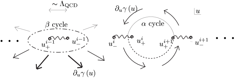
Figure 5: The two kinds of cycles and the behavior of the field strength $\partial_{u}\gamma\left(u\right)$.

In addition to the above type of the integral pass ($\beta$-cycle), there is also another type of the pass of the integral, called $\alpha$-cycle. This is the pass which runs around the points, say $(u_{+}^{(i)},u_{+}^{(i+1)})$ crossing the $i$th and $(i+1)$th branch cuts. (See Fig.5) By this $\alpha$-cycle integral for the field strength (53), we can easily see $\frac{1}{2\pi}\oint_{\alpha}\partial_{u}\gamma=0$. This means that there is no source from which the flux goes out. It leads to that the fluxes go around the $\alpha$-cycles from one branch cut to another branch cut.

Can we put the geometrical meaning on this $\gamma\left(u\right)$ ? We can interpret that this complex function expresses the point $(b^{{\rm NS}},-b^{{\rm R}})$ on the torus with constant complex structure $\tau=i/g_{s}+C_{0}$. In our analysis, we have to limit within the region, $g_{s}\ll 1$ and $b^{{\rm NS}}\ll 1$ with the arbitrary magnitude of the ratio, $b^{{\rm NS}}/g_{s}$. As a result of that, one of the two periods of this torus is finite and the other is infinite. This leads to the conclusion that this complex function $\gamma\left(u\right)$ expresses the arbitrary point in the belt-like two-dimensional plane with the topology ${\rm R}\times{\rm S^{1}}$. This also means that we do not have the complete invariance under the SL(2 Z) transformation $-$ there are the invariance under T-transformation which is originated from the periodicity of $x_{10}$-direction in M theory, but no invariance under S-transformation. Of course, we can directly see this fact from the form of this complex function.

We comment here on the Seiberg-Witten 1-form. This is written as $\lambda_{{\rm SW}}\equiv ud\gamma$ and gives us the exact expression for the effective gauge coupling constants of the low energy U(1)${}^{{\rm N}_{\rm c}-1}$ gauge theory of the 4D ${\cal N}=2$ SU(${\rm N}_{\rm c}$) gauge theory. The U(1) effective gauge coupling constant (perturbatively) corresponds to the value of the field $g_{s}^{-1}b^{{\rm NS}}$ at the point where each D5-brane is located. As seen in our discussion, this also gives the expression for the D3-charge induced in each D5-brane. So we can expect the exact result for the effective coupling constant will also give us the exact expression for the D3-brane charge. This is also the same in the case with fundamental matters if we replace $b^{{\rm NS}}$ with ${\tilde{b}^{{\rm NS}}}$. The calculation of these effective gauge coupling constants has been done a lot, so we do not repeat this analysis here. We limit our discussion within the comment on this.

In summary, the non-perturbative (D1-brane) effect will be speculated as below:

• The classical $\delta$ function-like singularities as the source of the D5 charge change into those of the branch cuts.

• There is the new type of ’flux’ which goes round between one branch cut and another branch cut.

Next, let us consider the case including the (massless) ${\rm N}_{\rm f}$ fundamental matters. This is almost the same as pure Yang-Mills case except that the Seiberg-Witten curve is different. This difference leads to the modification of $\gamma$ as

$$\gamma\left(u\right)=i(\ln y_{+}-\ln y_{-}),\hskip 28.45274pty_{\pm}\equiv\sum_{n=0}^{{\rm N}_{\rm c}}s_{n}u^{n}\pm\sqrt{\left(\sum s_{n}u^{n}\right)^{2}-\Lambda_{{\rm QCD}}^{2{\rm N}_{\rm c}-{\rm N}_{\rm f}}u^{{\rm N}_{\rm f}}}\ \ .$$ (54)

In the above, $y_{\pm}$ are the solution of the quadratic equation (Seiberg-Witten curve), $y+\Lambda_{{\rm QCD}}^{2{\rm N}_{\rm c}-{\rm N}_{\rm f}}u^{{\rm N}_{\rm f}}/y=2\sum_{n=0}^{{\rm N}_{\rm c}}s_{n}u^{n}$. Note that $y$ is not the same coordinate as that of pure SYM theory, but the same as that appeared in our analysis of the previous sections.

Let us rewrite the expression for $\gamma$ as

$$\gamma\left(u\right)=i\left\{2\ln\left(\frac{\sum_{n=0}^{{\rm N}_{\rm c}}s_{n}u^{n}+\sqrt{\left(\sum s_{n}u^{n}\right)^{2}-\Lambda_{{\rm QCD}}^{2{\rm N}_{\rm c}-{\rm N}_{\rm f}}u^{{\rm N}_{\rm f}}}}{\Lambda_{{\rm QCD}}^{{\rm N}_{\rm c}}}\right)-{\rm N}_{\rm f}\ln\left(\frac{u}{\Lambda_{{\rm QCD}}}\right)\right\}.$$ (55)

It is easy to see from the first term that there are ${\rm N}_{\rm c}$ singularities of the branch cuts. Roughly speaking, this shows that classical $\delta$ function-like singularities of the external ${\rm N}_{\rm c}$ D5-brane source changes into those of the branch cuts. The second statement in pure SYM theory about the two kinds of flux is also applicable to this case with matters. But we have to be careful of the second term in the above expression for $\gamma\left(u\right)$. This gives additional contribution of $-{\rm N}_{\rm f}$ D5 charge to the contour integral around the origin. So we can roughly say that this term is the contribution of the matters or the background, as compared with the first term. In fact, in the region $|u|\gg\Lambda_{{\rm QCD}}$, we can see the behavior of $\gamma\left(u\right)$ with the vanishing moduli $\{s_{n}\}=0$, as

$$\gamma\left(u\right)\sim i\left(2{\rm N}_{\rm c}-{\rm N}_{\rm f}\right)\ln\left(\frac{u}{\Lambda_{{\rm QCD}}}\right),$$ (56)

where the first term in the above comes from the first term of Eq.(55). This is the perturbative RG-flow in the ultraviolet region in the 4D field theory.

Note that we can also obtain this result in the gentler region $|u|/\Lambda_{{\rm QCD}}>1$ by the large ${\rm N}_{\rm c}$ and ${\rm N}_{\rm f}$ limit. This is the RG-flow in the region where AdS/CFT correspondence is effective as discussed in section 6.

Therefore as long as one of the above conditions is satisfied, our result for the complex field in the previous sections is trustworthy.

Appendix

In this appendix, we will show our analysis in the section 3.1 and 3.2 is the same when we start from the Born-Infeld action.

After taking the static gauge $\sigma_{0}=t$ and $\{\sigma_{4},\sigma_{5}\}=\{x_{4},x_{5}\}$, and assuming that only $X^{6}=X^{6}(x_{4},x_{5})$ and $A_{0}=A_{0}(x_{4},x_{5})$ are the nontrivial fields, let us take the limit (6). Then the action (11) reduces to

$$S_{{\rm D2}}^{{\rm BI}} = -\frac{1}{4\pi\Lambda}\int dtdu^{4}du^{5}{\rm H}\left\{{\rm G}\left(\vec{\nabla}_{u}\phi,\vec{\nabla}_{u}a\right)\right\}^{1/2}+\frac{\Lambda^{2}}{4\pi}\int dtdu^{4}du^{5}\frac{{\rm N}_{\rm f}}{R^{2}}\left(\frac{\phi}{R}-\vec{\nabla}_{u}\phi\cdot\frac{\vec{u}}{R}\right)a,$$ (57)

$${\rm G}\equiv{\rm G}\left(\vec{\nabla}_{u}\phi,\vec{\nabla}_{u}a\right)\equiv 1+\Lambda^{2}\left\{\left|\vec{\nabla}_{u}\phi\right|^{2}-\left|\vec{\nabla}_{u}a\right|^{2}\right\}-\Lambda^{4}\left(\vec{\nabla}_{u}\phi\times\vec{\nabla}_{u}a\right)^{2}$$

where we use the same convention in the section 3.1. Let us add the source with $\pm{\rm N}_{\rm c}$ electric charges to the above action. From the action $S_{{\rm D2}}^{{\rm BI}}+\Delta S$, we can see the constraint for $a$ (Gauss-Low),

$$\vec{\nabla}_{u}\left({\rm HG^{\frac{-1}{2}}}\vec{\nabla}_{u}a\right)+\Lambda^{2}\vec{\nabla}_{u}\times\left\{{\rm HG^{\frac{-1}{2}}}\vec{\nabla}_{u}\phi\left(\vec{\nabla}_{u}a\times\vec{\nabla}_{u}\phi\right)\right\}=\frac{{\rm N}_{\rm f}\Lambda}{R^{3}}\left(\phi-\vec{\nabla}_{u}\phi\cdot\vec{u}\right)\pm 4\pi{\rm N}_{\rm c}\delta(u^{4})\delta(u^{5})$$

$$\hskip 170.71652pt=\vec{\nabla}_{u}\left(-\frac{{\rm N}_{\rm f}\Lambda\phi}{R}\frac{\vec{u}}{|u|^{2}}+\left\{{\rm sign}(\phi_{0}){\rm N}_{\rm f}\pm 2{\rm N}_{\rm c}\right\}\frac{\vec{u}}{|u|^{2}}\right),$$ (58)

where the right hand is the same as that of the section 3.1. Next, let us consider the equation of motion. We can easily obtain

$$\vec{\nabla}_{u}\left({\rm HG^{\frac{-1}{2}}}\vec{\nabla}_{u}\phi\right)-\Lambda^{2}\vec{\nabla}_{u}\times\left\{{\rm HG^{\frac{-1}{2}}}\vec{\nabla}_{u}a\left(\vec{\nabla}_{u}\phi\times\vec{\nabla}_{u}a\right)\right\}=-\frac{{\rm N}_{\rm f}\Lambda}{R^{3}}\left({\rm G^{\frac{-1}{2}}}\phi+\vec{\nabla}_{u}a\cdot\vec{u}\right)\mp 4\pi{\rm N}_{\rm c}\delta^{2}({\vec{u}}).$$

From this form, we can see that the same additional relation $\vec{\nabla}a=-\vec{\nabla}\phi$ which appears in the section 3.1. make the above equation equivalent to the Gauss-Low (58). As a result of that, we obtain the same equation as Eq.(17) to determine the behavior of $\phi$ as that of the section 3.1.

Then let us discuss the field $\chi$. The electric charge ${\rm Q_{E}}$ in this case is given by the integral of the left hand as

$${\rm Q_{E}}=\frac{1}{4\pi}\oint*\left\{{\rm HG^{\frac{-1}{2}}}\vec{\nabla}_{u}a+\Lambda^{2}{\rm HG^{\frac{-1}{2}}}\tilde{\nabla}_{u}\phi\left(\vec{\nabla}\phi\times\vec{\nabla}a\right)+{\rm N}_{\rm f}\left(\frac{\Lambda\phi}{R}-{\rm sign}(\phi_{0})\right)\frac{{\vec{u}}}{|u|^{2}}\right\}=\pm{\rm N}_{\rm c},$$

By taking the current of $\phi_{0}>0$ as the standard. we define the ’dual’ field $\chi$ as

$$\tilde{\nabla}_{u}\chi\equiv{\rm HG^{\frac{-1}{2}}}\vec{\nabla}_{u}a+\Lambda^{2}{\rm HG^{\frac{-1}{2}}}\tilde{\nabla}_{u}\phi\left(\vec{\nabla}\phi\times\vec{\nabla}a\right)+{\rm N}_{\rm f}\left(\frac{\Lambda\phi}{R}-1\right)\frac{{\vec{u}}}{|u|^{2}}$$ (59)

By this definition, we can see the solution for $\chi$ is the same as (24).

In summary, the final result for $\phi$ and $\chi$ are the same as those of the section 3.1 even when we start with the Born-Infeld action (57).

References

- [1] J. Maldacena, The large N limit of superconformal field theories and supergravity, Adv. Theor. Math. Phys. 2(1998) 231, hep-th/9711200.
- [2] Igor R. Klebanov, Nikita A. Nekrasov, Gravity Duals of Fractional Branes and Logarithmic RG Flow, Nucl.Phys. B574 (2000) 263-274, hep-th/9911096.
- [3] M. Bertolini, P. Di Vecchia, M. Frau, A. Lerda, R. Marotta, I. Pesando, Fractional D-branes and their gauge duals, JHEP 0102 (2001) 014, hep-th/0011077.
- [4] I.R. Klebanov, A.A. Tseytlin, Gravity Duals of Supersymmetric SU(N) x SU(N+M) Gauge Theories, Nucl.Phys. B578 (2000) 123-138, hep-th/0002159.
- [5] Juan Maldacena, Carlos Nunez, Supergravity description of field theories on curved manifolds and a no go theorem, Int.J.Mod.Phys. A16 (2001) 822-855, hep-th/0007018.
- [6] Bjorn Brinne, Ansar Fayyazuddin, Subir Mukhopadhyay, Douglas J. Smith, Supergravity M5-branes wrapped on Riemann surfaces and their QFT duals, JHEP 0012 (2000) 013, hep-th/0009047.
- [7] Joseph Polchinski, N = 2 Gauge/Gravity Duals, Int.J.Mod.Phys. A16 (2001) 707-718, hep-th/0011193.
- [8] A. Rajaraman, Supergravity Duals for N=2 Gauge Theories, hep-th/0011279.
- [9] M. Petrini, R. Russo, A. Zaffaroni, N=2 Gauge Theories and Systems with Fractional Branes Nucl.Phys. B608 (2001) 145-161, hep-th/0104026.
- [10] M. Billo’, L. Gallot, A. Liccardo, Classical geometry and gauge duals for fractional branes on ALE orbifolds, Nucl.Phys. B614 (2001) 254-278, hep-th/0105258.
- [11] Jerome P. Gauntlett, Nakwoo Kim, Dario Martelli, Daniel Waldram, Wrapped fivebranes and N=2 super Yang-Mills theory, Phys.Rev. D64 (2001) 106008, hep-th/0106117.
- [12] F. Bigazzi, A. L. Cotrone, A. Zaffaroni, N=2 Gauge Theories from Wrapped Five-branes, Phys.Lett. B519 (2001) 269-276, hep-th/0106160
- [13] M. Bertolini, V. L. Campos, G. Ferretti, P. Fre’, P. Salomonson, M. Trigiante, Supersymmetric 3-branes on smooth ALE manifolds with flux, hep-th/0106186.
- [14] P. Bain, Fractional D3-branes in diverse backgrounds, hep-th/0112145.
- [15] P. Di Vecchia, A. Lerda, P. Merlatti N=1 and N=2 Super Yang-Mills theories from wrapped branes, hep-th/0205204.
- [16] Mariana Grana, Joseph Polchinski, Gauge/Gravity Duals with Holomorphic Dilaton, Phys.Rev. D65 (2002) 126005, hep-th/0106014.
- [17] M. Bertolini, P. Di Vecchia, M. Frau, A. Lerda, R. Marotta, N=2 Gauge theories on systems of fractional D3/D7 branes, Nucl.Phys. B621 (2002) 157-178, hep-th/0107057.
- [18] Edward Witten, Solutions Of Four-Dimensional Field Theories Via M Theory, Nucl.Phys. B500 (1997) 3-42, hep-th/9703166.
- [19] Joseph Polchinski, TASI Lectures on D-Branes, hep-th/9611050.
- [20] Angel M. Uranga, Brane Configurations for Branes at Conifolds, JHEP 9901 (1999) 022, hep-th/9811004.
- [21] Keshav Dasgupta, Sunil Mukhi, Brane Constructions, Conifolds and M-Theory, Nucl.Phys. B551 (1999) 204-228, hep-th/9811139.
- [22] Ansar Fayyazuddin, Douglas J. Smith, Localized intersections of M5-branes and four-dimensional superconformal field theories, JHEP 9904 (1999) 030, hep-th/9902210.
- [23] A. Lawrence, N. Nekrasov, C. Vafa, On Conformal Theories in Four Dimensions, Nucl.Phys. B533 (1998) 199-209, hep-th/9803015.
- [24] Amihay Hanany, Edward Witten, Type IIB Superstrings, BPS Monopoles, And Three-Dimensional Gauge Dynamics, Nucl.Phys. B492 (1997) 152-190, hep-th/9611230.
- [25] Joaquim Gomis, Paul K. Townsend, Mattias, N.R. Wohlfarth, The ‘s-rule’ exclusion principle and vacuum interpolation in worldvolume dynamics, hep-th/0211020.
- [26] John H. Schwarz, An SL(2,Z) Multiplet of Type IIB Superstrings, Phys.Lett. B360 (1995) 13-18; Erratum-ibid. B364 (1995) 252, hep-th/9508143.
- [27] Toshio Nakatsu, Kazutoshi Ohta, Takashi Yokono, Yuhsuke Yoshida, Higgs Branch of N=2 SQCD and M theory Branes, Nucl.Phys. B519 (1998) 159-179, hep-th/9707258.
- [28] Michael R. Douglas, Gregory Moore, D-branes, Quivers, and ALE Instantons, hep-th/9603167
- [29] Yosuke Imamura, Supersymmetries and BPS Configurations on Anti-de Sitter Space, Nucl.Phys. B537 (1999) 184-202, hep-th/9807179.
- [30] Curtis G. Callan, Alberto Guijosa, Konstantin G. Savvidy, Baryons and String Creation from the Fivebrane Worldvolume Action, Nucl.Phys. B547 (1999) 127-142, hep-th/9810092.
- [31] J. M. Camino, A. V. Ramallo, J. M. Sanchez de Santos, Worldvolume Dynamics of D-branes in a D-brane Background, Nucl.Phys. B562 (1999) 103-132, hep-th/9905118.
- [32] J. M. Camino, A. Paredes, A.V. Ramallo, Stable Wrapped Branes, JHEP 0105 (2001) 011, hep-th/0104082.
- [33] C.P. Bachas, M.B. Green, A Classical Manifestation of the Pauli Exclusion Principle, JHEP 9801 (1998) 015, hep-th/9712187.
- [34] Michael Green, Jeffrey A. Harvey, Gregory Moore, I-Brane Inflow and Anomalous Couplings on D-Branes, Class.Quant.Grav. 14 (1997) 47-52, hep-th/9605033.
- [35] Curtis G. Callan, Jr., Juan M. Maldacena, Brane Dynamics From the Born-Infeld Action, Nucl.Phys. B513 (1998) 198-212, hep-th/9708147
- [36] R.C. Myers, Dielectric-Branes, JHEP 9912 (1999) 022, hep-th/9910053.
- [37] Nissan Itzhaki, Juan M. Maldacena, Jacob Sonnenschein, Shimon Yankielowicz, Supergravity and The Large N Limit of Theories With Sixteen Supercharges, Phys.Rev. D58 (1998) 046004, hep-th/9802042.
- [38] Akikazu Hashimoto, Supergravity Solutions for Localized Intersections of Branes, JHEP 9901 (1999) 018, hep-th/9812159.
- [39] Paul S. Aspinwall, K3 Surfaces and String Duality, hep-th/9611137.
- [40] Nick Dorey, Timothy J. Hollowood, Valentin V. Khoze, Michael P. Mattis, The Calculus of Many Instantons, hep-th/0206063.
- [41] J.L.F. Barbon, A. Pasquinucci, D0-Branes, Constrained Instantons and D=4 Super Yang-Mills Theories, Nucl.Phys. B517 (1998) 125-141, hep-th/9708041.
- [42] John Brodie, Fractional Branes, Confinement, and Dynamically Generated Superpotentials, Nucl.Phys. B532 (1998) 137-152, hep-th/9803140.
- [43] M. Wijnholt and S. Zhukov, Inside an Enhankon: Monopoles and Dual Yang-Mills Theory, Nucl.Phys. B639 (2002) 343-369, hep-th/0110109.