Fermions on the light front transverse lattice

Abstract

We address the problems of fermions in light front QCD on a transverse lattice. We propose and numerically investigate different approaches of formulating fermions on the light front transverse lattice. In one approach we use forward and backward derivatives. There is no fermion doubling and the helicity flip term proportional to the fermion mass in the full light front QCD becomes an irrelevant term in the free field limit. In the second approach with symmetric derivative (which has been employed previously in the literature), doublers appear and their occurrence is due to the decoupling of even and odd lattice sites. We study their removal from the spectrum in two ways namely, light front staggered formulation and the Wilson fermion formulation. The numerical calculations in free field limit are carried out with both fixed and periodic boundary conditions on the transverse lattice and finite volume effects are studied. We find that an even-odd helicity flip symmetry on the light front transverse lattice is relevant for fermion doubling.

I Introduction

Light front Hamiltonian formulation of transverse lattice QCD Bardeen:1976tm ; Bardeen:1980xx has many interesting features. With the gauge choice $A^{+}=A^{0}+A^{3}=0$ and the elimination of the constrained variable $A^{-}=A^{0}-A^{3}$, it uses minimal gauge degrees of freedom in a manifestly gauge invariant formulation exploiting the residual gauge symmetry in this gauge. So far encouraging results have been obtained in the pure gauge sector and in the meson sector with particle number truncation (for a recent review see, Ref. review ).

It is well known that fermions on the lattice pose challenging problems due to the doubling phenomenon. Light front formulation of field theory has its own peculiarities concerning fermions because of the presence of a constraint equation. As an example, the usual chiral transformation on the four component fermion field is incompatible with the constraint equation for nonzero fermion mass Wilson:1994fk . There have been previous studies of fermions on the transverse lattice stagger ; BK ; dalme ; buseal . Our approach in this work is quite extensive and aims to understand the origin of the doublers. We identify an even-odd helicity flip symmetry of the light front transverse lattice Hamiltonian, absence of which means removal of doublers in all the cases we have studied. This is closely related to the need to break chiral symmetry explicitly in the usual Euclidean formulation of lattice fermions.

As we shall see later in this article, the presence of the constraint equation in light front field theory allows different methods to put fermions on a transverse lattice. It is worthwhile to study all the different methods in order to examine their strengths and weaknesses. In this work, we carry out a detailed numerical investigation of three methods in free field limit with special emphasis on finite volume effects. We also study the effects of imposing fixed and periodic boundary conditions which have significant effects in finite volumes. There are two important reasons to thoroughly study finite volume effects. First, for a reasonable size of Fock space, computing limitations will force us to be in a reasonably small volume when we deal with realistic problems. Second, the currently practiced version of the transverse lattice gauge theory uses linear link variables and recovering continuum physics is nontrivial. Finite volume studies are also important in this connection.

In one of the approaches of treating fermions on the light front transverse lattice, we maintain as much transverse locality as possible on the lattice by using forward and backward derivatives without spoiling the hermiticity of the Hamiltonian. In this case doublers are not present and the helicity flip term proportional to the fermion mass in the full light front QCD becomes an irrelevant term in the free field limit. Thus in finite volume, depending on the boundary condition used, the two helicity states of the fermion may not be degenerate in the free field limit. However, we find that in the infinite volume limit the degeneracy is restored irrespective of the boundary condition.

In the second approach BK , symmetric derivatives are used which results in a Hamiltonian with only next to nearest neighbor interaction when we take the free field limit. As a consequence even and odd lattice sites decouple and the fermions live independently of each other on the two sets of sites. As a result we get four species of fermions on a two dimensional lattice as excitations around zero transverse momentum (Note that this is quite different from what one gets in the conventional Euclidean lattice theory when one uses symmetric derivatives. In that case, doublers have at least one momentum component near the edge of the Brillouin zone.). The doublers can be removed in more than one way. We propose to use the staggered fermion formulation on the light front transverse lattice to eliminate two doublers and reinterpret the remaining two as two flavors. In this light front staggered fermion formulation, there is no flavor mixing in free field limit. But, in QCD, we get irrelevant flavor mixing terms. An alternative which removes doubling completely is to add the conventional Wilson term which generates many irrelevant interactions on the transverse lattice. Among them, the helicity flip interactions vanish but the helicity non flip interactions survive in the free field limit.

The plan of this paper is as follows. Notation and conventions are presented in Sec. II. QCD Hamiltonian with forward-backward derivative is discussed and free field limit is studied in Sec. III. QCD Hamiltonian with symmetric derivative with its free field limit is considered in Sec. IV. Staggered formulation and reinterpretation of doublers are discussed in Sec. V. Removal of doublers via the Wilson term is studied in Sec. VI. We discuss the even-odd spin flip symmetry and its relation to the fermion doubling on the light front transverse lattice in Sec. VII. Finally Sec. VIII contains summary and conclusions. In appendix A we compare and contrast the forward-backward derivative in conventional lattice and light front transverse lattice for free fermion field theory.

II Light Front Preliminaries

II.1 Notation and conventions

The light front coordinates are $x^{\pm}=x^{0}\pm x^{3}$, $x^{\perp}=(x^{1},x^{2})$, the partial derivative $\partial^{\pm}=2{\partial\over\partial x^{\mp}}$, the gamma matrices $\gamma^{\pm}=\gamma^{0}\pm\gamma^{3}$ and projection operators $\Lambda^{\pm}={1\over 4}\gamma^{\mp}\gamma^{\pm}$ . $x^{+}$ is the light front time and $x^{-}$ is the light front longitudinal coordinate.

The Lagrangian density for the free fermion is

$${\cal L}_{free}={\bar{\psi}}(i\gamma^{\mu}\partial_{\mu}-m)\psi.$$ (1)

Going to light front coordinates and using $\psi^{\pm}=\Lambda^{\pm}\psi$,

$${\cal L}_{free}={\psi^{+}}^{\dagger}i\partial^{-}\psi^{+}+{\psi^{-}}^{\dagger}i\partial^{+}\psi^{-}-{\psi^{-}}^{\dagger}(i\alpha^{\perp}\cdot\partial^{\perp}+\gamma^{0}m)\psi^{+}-{\psi^{+}}^{\dagger}(i\alpha^{\perp}\cdot\partial^{\perp}+\gamma^{0}m)\psi^{-}~{}.$$ (2)

One of the equations of motion from the above free Lagrangian is

$$i\partial^{+}\psi^{-}=(i\alpha^{\perp}\cdot\partial^{\perp}+\gamma^{0}m)\psi^{+},$$ (3)

which is actually a constraint equation because of absence of a time derivative.

$\psi^{+}$ is the dynamical fermion field and its equation of motion is given by

$$i\partial^{-}\psi^{+}=(i\alpha^{\perp}\cdot\partial^{\perp}+\gamma^{0}m)\psi^{-}.$$ (4)

One can remove $\psi^{-}$ from Eq. (4) using the constraint equation (Eq. (3)). The dynamical field $\psi^{+}$ can essentially be represented by two components hz such that

$$\psi^{+}(x^{-},x^{\perp})=\left[\begin{array}[]{l}\eta(x^{-},x^{\perp})\\ 0\end{array}\right],$$ (7)

where $\eta$ is a two component field. Its Fock expansion in the light front quantization with tranverse directions discretized on a two dimensional square lattice is given by

$$\eta(x^{-},{\bf x})=\sum_{\lambda}\chi_{\lambda}\int{dk^{+}\over 2(2\pi)\sqrt{k^{+}}}\big{[}b(k^{+},{\bf x},\lambda)e^{-{i\over 2}k^{+}x^{-}}+d^{\dagger}(k^{+},{\bf x},-\lambda)e^{{i\over 2}k^{+}x^{-}}\Big{]},$$ (8)

where $\chi_{\lambda}$ is the Pauli spinor, $\lambda=1,2$ denotes two helicity states. ${\bf x}$ now denotes the transverse lattice points.

The canonical commutation relations are

$$\{b(k^{+},{\bf x},\lambda),b^{\dagger}({k^{\prime}}^{+},{\bf x}^{\prime},\lambda^{\prime})\} = \{d(k^{+},{\bf x},\lambda),d^{\dagger}({k^{\prime}}^{+},{\bf x}^{\prime},\lambda^{\prime})\}$$ (9)

$$= 2(2\pi)k^{+}~{}\delta(k^{+}-{k^{\prime}}^{+})~{}\delta_{\lambda\lambda^{\prime}}~{}\delta_{{\bf x},{\bf x}^{\prime}}~{}.$$

Using $\int_{-\infty}^{+\infty}dk^{+}e^{{i\over 2}k^{+}(x^{-}-y^{-})}=2(2\pi)\delta(x^{-}-y^{-})$, we have,

$$\Big{\{}\eta(x^{-},{\bf x}),\eta^{\dagger}(y^{-},{\bf x}^{\prime})\Big{\}}=\openone~{}\delta_{{\bf x},{\bf x}^{\prime}}~{}\delta(x^{-}-y^{-})$$ (10)

where $\openone$ is a 2 by 2 unit matrix.

We use Discretized Light Cone Quantization (DLCQ) BPP for the longitudinal dimension ($-L\leq x^{-}\leq+L$) and implement anti periodic boundary condition to avoid zero modes. Then,

$$\eta(x^{-},{\bf x})={1\over\sqrt{2L}}\sum_{\lambda}\chi_{\lambda}\sum_{l=1,3,5,\dots}[b(l,{\bf x},\lambda)e^{-i{\pi lx^{-}/(2L)}}+d^{\dagger}(l,{\bf x},-\lambda)e^{i{\pi lx^{-}/(2L)}}]$$ (11)

with

$$\{b(l,{\bf x},\lambda),b^{\dagger}(l^{\prime},{\bf x}^{\prime},\lambda^{\prime})\}=\{d(l,{\bf x},\lambda),d^{\dagger}(l^{\prime},{\bf x}^{\prime},\lambda^{\prime})\}=\delta_{ll^{\prime}}\delta_{{\bf x},{\bf x}^{\prime}}~{}\delta_{\lambda,\lambda^{\prime}}.$$ (12)

In DLCQ with antiperiodic boundary condition, it is usual to multiply the Hamiltonian $P^{-}$ by ${\pi\over L}$, so that $H={\pi\over L}P^{-}$ has the dimension of mass squared.

In the following, for notational convenience we suppress $x^{-}$ in the arguments of the fields.

III Hamiltonian with forward and backward derivatives

III.1 Construction

The fermionic part of the Lagrangian density is

$${\cal L}_{f}={\bar{\psi}}(i\gamma^{\mu}D_{\mu}-m)\psi$$ (13)

with $iD^{\mu}=i\partial^{\mu}-gA^{\mu}$.

Moving to the light front coordinates, using the $A^{+}=0$ gauge and introducing the transverse lattice,

$${\cal L}_{f} = {\psi^{+}}^{\dagger}(i\partial^{-}-gA^{-})\psi^{+}+{\psi^{-}}^{\dagger}i\partial^{+}\psi^{-}$$ (14)

$$-i{\psi^{-}}^{\dagger}\alpha_{r}D^{f}_{r}\psi^{+}-i{\psi^{+}}^{\dagger}\alpha_{r}D^{b}_{r}\psi^{-}$$

$$-m{\psi^{-}}^{\dagger}\gamma^{0}\psi^{+}-m{\psi^{+}}^{\dagger}\gamma^{0}\psi^{-}.$$

Here $r=1,2$ and $D^{f/b}_{r}$ is the forward/backward covariant lattice derivative. Our goal here is to write the most local lattice derivative. That is why, instead of using the symmetric lattice derivative, in the above we have used the forward and backward lattice derivatives. However, the Hermiticity of the Lagrangian (Hamiltonian) requires that if one of the covariant lattice derivatives appearing in Eq. (14) is the forward derivative, the other has to be the backward derivative or vice versa. The covariant forward and backward derivatives on the lattice are defined as

$$D_{r}^{f}\eta({\bf x})={1\over a}[U_{r}({\bf x})\eta({\bf x}+a{\hat{\bf r}})-\eta({\bf x})]$$ (15)

and

$$D_{r}^{b}\eta({\bf x})={1\over a}[\eta({\bf x})-U_{r}^{\dagger}({\bf x}-a{\hat{\bf r}})\eta({\bf x}-a{\hat{\bf r}})],$$ (16)

where $a$ is the lattice constant and ${\hat{\bf r}}$ is unit vector in the direction $r=1,2$ and ${D^{f}_{r}}^{\dagger}=-D^{b}_{r}$. $U_{r}({\bf x})$ is the group valued lattice gauge field with the property $U_{r}^{\dagger}({\bf x})=U_{-r}({\bf x}+a{\hat{\bf r}})$. Using the constraint equation

$$i\partial^{+}\psi^{-}=(i\alpha_{r}D^{f}_{r}+\gamma^{0}m)\psi^{+},$$ (17)

and finally going over to the two component fields $\eta$

$${\cal L}_{f} = {\psi^{+}}^{\dagger}(i\partial^{-}-gA^{-})\psi^{+}-m{\psi^{+}}^{\dagger}\gamma^{0}\psi^{-}-i{\psi^{+}}^{\dagger}\alpha_{r}D^{b}_{r}\psi^{-}$$

$$= {\psi^{+}}^{\dagger}(i\partial^{-}-gA^{-})\psi^{+}$$

$$~{}~{}~{}~{}-{\psi^{+}}^{\dagger}[i\alpha_{r}D^{b}_{r}+\gamma^{0}m]{1\over i\partial^{+}}[i\alpha_{s}D^{f}_{s}+\gamma^{0}m]\psi^{+}$$

$$= {\eta}^{\dagger}(i\partial^{-}-gA^{-})\eta$$

$$~{}~{}~{}~{}-\eta^{\dagger}[i{\hat{\sigma}}_{r}D^{b}_{r}-im]{1\over i\partial^{+}}[i{\hat{\sigma}}_{s}D^{f}_{s}+im]\eta~{}.$$

${\hat{\sigma}_{1}}=\sigma_{2}$ and ${\hat{\sigma}_{2}}=-\sigma_{1}$. So, we arrive at the Lagrangian density

$${\cal L}_{f} = \eta^{\dagger}(i\partial^{-}-gA^{-})\eta-m^{2}\eta^{\dagger}{1\over i\partial^{+}}\eta$$ (19)

$$~{}~{}-m\eta^{\dagger}({\bf x})\sum_{r}{\hat{\sigma}}_{r}{1\over a}{1\over i\partial^{+}}\Big{[}U_{r}({\bf x})\eta({\bf x}+a{\hat{\bf r}})-\eta({\bf x})\Big{]}$$

$$~{}~{}-m\sum_{r}\Big{[}\eta^{\dagger}({\bf x}+a{\hat{\bf r}})U_{r}^{\dagger}({\bf x})-\eta^{\dagger}({\bf x})\Big{]}{\hat{\sigma}}_{r}{1\over a}{1\over i\partial^{+}}\eta({\bf x})$$

$$~{}-{1\over a^{2}}\sum_{r}[\eta^{\dagger}({\bf x}+a{\hat{\bf r}})U_{r}^{\dagger}({\bf x})-\eta^{\dagger}({\bf x})]{\hat{\sigma}}_{r}{1\over i\partial^{+}}{\hat{\sigma}}_{s}[U_{s}({\bf x})\eta({\bf x}+a{\hat{\bf s}})-\eta({\bf x})].$$

In the free limit the fermionic part of the Hamiltonian becomes

$$P^{-}_{fb} = \int dx^{-}a^{2}\sum_{{\bf x}}{\cal H}$$ (20)

$$= \int dx^{-}a^{2}\sum_{{\bf x}}\Bigg{[}m^{2}\eta^{\dagger}({\bf x}){1\over i\partial^{+}}\eta({\bf x})$$

$$~{}~{}~{}~{}-{1\over a^{2}}\eta^{\dagger}({\bf x})\sum_{r}{1\over i\partial^{+}}[\eta({\bf x}+a{\hat{\bf r}})-2\eta({\bf x})+\eta({\bf x}-a{\hat{\bf r}})$$

$$~{}~{}~{}~{}+{1\over a^{2}}\eta^{\dagger}({\bf x})\sum_{r}(am{\hat{\sigma}_{r}}){1\over i\partial^{+}}[\eta({\bf x}+a{\hat{\bf r}})-2\eta({\bf x})+\eta({\bf x}-a{\hat{\bf r}})]\Bigg{]}.$$

In order to get Eq. (20), we have assumed infinite transverse lattice and accordingly have used shifting of lattice points. The positive sign in front of the last term would change if we had switched forward and backward derivatives.

Because of the presence of ${\hat{\sigma}}_{r}$ the last term of Eq. (20) couples fermions of opposite helicities. Note that it is also linear in mass. Such a helicity flip linear mass term is typical in continuum light front QCD. Here in free transverse lattice theory this term arises from the interference of the first order derivative term and the mass term, due to the constraint equation. This is in contrast to the conventional lattice (see Appendix A) where no helicity flip or chirality-mixing term arises in the free theory if we use forward and backward lattice derivatives.

In DLCQ the Hamiltonian is given by,

$$H_{fb}=H_{0}+H_{hf}$$ (21)

where

$$H_{0} = \sum_{{\bf z}}\sum_{\lambda}\sum_{l}{a^{2}m^{2}\over l}\left[b^{\dagger}(l,{\bf z},\lambda)b(l,{\bf z},\lambda)+d^{\dagger}(l,{\bf z},\lambda)d(l,{\bf z},\lambda)\right]$$ (22)

$$-\sum_{{\bf z}}\sum_{r}\sum_{\lambda}\sum_{\lambda^{\prime}}\sum_{l}{1\over l}{\chi^{\dagger}}_{\lambda^{\prime}}\chi_{\lambda}$$

$$\Big{[}b^{\dagger}(l,{\bf z},\lambda^{\prime})b(l,{\bf z}+a{\hat{\bf r}},\lambda)-2b^{\dagger}(l,{\bf z},\lambda^{\prime})b(l,{\bf z},\lambda)+b^{\dagger}(l,{\bf z},\lambda^{\prime})b(l,{\bf z}-a{\hat{\bf r}},\lambda)$$

$$+d^{\dagger}(l,{\bf z},\lambda^{\prime})d(l,{\bf z}+a{\hat{\bf r}},\lambda)-2d^{\dagger}(l,{\bf z},\lambda^{\prime})d(l,{\bf z},\lambda)+d^{\dagger}(l,{\bf z},\lambda^{\prime})d(l,{\bf z}-a{\hat{\bf r}},\sigma)\Big{]}$$

and

$$H_{hf} = \sum_{{\bf z}}\sum_{r}\sum_{\lambda}\sum_{\lambda^{\prime}}\sum_{l}{1\over l}{\chi^{\dagger}}_{\lambda^{\prime}}[am{\hat{\sigma}}^{r}]\chi_{\lambda}$$

$$\Big{[}b^{\dagger}(l,{\bf z},\lambda^{\prime})b(l,{\bf z}+a{\hat{\bf r}},\lambda)-2b^{\dagger}(l,{\bf z},\lambda^{\prime})b(l,{\bf z},\lambda)+b^{\dagger}(l,{\bf z},\lambda^{\prime})b(l,{\bf z}-a{\hat{\bf r}},\lambda)$$

$$+d^{\dagger}(l,{\bf z},\lambda^{\prime})d(l,{\bf z}+a{\hat{\bf r}},\lambda)-2d^{\dagger}(l,{\bf z},\lambda^{\prime})d(l,{\bf z},\lambda)+d^{\dagger}(l,{\bf z},\lambda^{\prime})d(l,{\bf z}-a{\hat{\bf r}},\sigma)\Big{]}.$$

III.2 Absence of doubling

Consider the Fourier transform in transverse space

$$\eta(x^{-},{\bf x})=\int{d^{2}k\over(2\pi)^{2}}e^{i{\bf k}\cdot{\bf x}}\phi_{\bf k}(x^{-})$$ (24)

where $-{\pi\over a}\leq k_{1},k_{2}\leq+{\pi\over a}$. Then the helicity nonflip part of Eq. (20) becomes

$$P^{-}_{nf}=\int dx^{-}\int{d^{2}k\over(2\pi)^{2}}\int{d^{2}p\over(2\pi)^{2}}\phi^{\dagger}_{\bf k}(x^{-}){1\over i\partial^{+}}\phi_{\bf p}(x^{-})a^{2}\sum_{\bf x}e^{-i({\bf k}-{\bf p})\cdot{\bf x}}\Bigg{[}m^{2}-\sum_{r}{1\over a^{2}}\Big{[}e^{i{\bf p}\cdot a{\hat{\bf r}}}-2+e^{-i{\bf p}\cdot a{\hat{\bf r}}}\Big{]}\Bigg{]}.$$ (25)

Using

$$a^{2}\sum_{\bf x}e^{i({\bf k}-{\bf p})\cdot{\bf x}}=(2\pi)^{2}~{}\delta^{2}({\bf k}-{\bf p})$$ (26)

we get,

$$P^{-}_{nf}=\int dx^{-}\int{d^{2}k\over(2\pi)^{2}}\phi^{\dagger}_{\bf k}(x^{-}){1\over i\partial^{+}}\phi_{\bf k}(x^{-})\Bigg{[}m^{2}+\sum_{r}k_{r}^{2}\left({\sin~{}k_{r}a/2\over k_{r}a/2}\right)^{2}\Bigg{]}$$ (27)

where we have defined $k_{r}a={\bf k}\cdot{\hat{\bf r}}a$. Note that the $sine$ function vanishes at the origin $k_{1},k_{2}=0$ but does not vanish at the edges of the Brillouin zone $k_{1},k_{2}=\pm{\pi\over a}$.

Define ${\tilde{k}}_{r}=k_{r}{\sin~{}k_{r}a/2\over k_{r}a/2}$. In the naive continuum limit ${\tilde{k}}_{r}\rightarrow k_{r}$.

Now, let us consider the full Hamiltonian (20) including the helicity flip term. In the helicity space we have the following matrix structure for $P^{+}P^{-}$ (since $P^{-}$ is inversely proportional to the total longitudinal momentum $P^{+}$, we study the operator $P^{+}P^{-}$)

$$\pmatrix{m^{2}+{4\over a^{2}}\sum_{r}\sin^{2}{k_{r}a\over 2}&-{4m\over a}(i\sin^{2}{k_{x}a\over 2}+\sin^{2}{k_{y}a\over 2}\cr&\cr{4m\over a}(i\sin^{2}{k_{x}a\over 2}-\sin^{2}{k_{y}a\over 2})&m^{2}+{4\over a^{2}}\sum_{r}\sin^{2}{k_{r}a\over 2}}$$ (28)

which leads to the eigenvalue equation

$${\cal M}^{2}=m^{2}+{4\over a^{2}}\sum_{r}\sin^{2}{k_{r}a\over 2}\pm{4m\over a}\sqrt{\sum_{r}\sin^{4}{k_{r}a\over 2}}.$$ (29)

Third term in the above equation comes from the linear mass helicity flip term. If the mass $m=0$, then it is obvious from Eq. (29) that ${\cal M}^{2}=0$ if and only if $k_{1}=k_{2}=0$. For nonzero $m$, one can also in general conclude that ${\cal M}^{2}=m^{2}$ only for the case $k_{1}=k_{2}=0$. Thus there are no fermion doublers in this case (for physical masses $am<1$). In the following for specific choices of momenta we elaborate on this further.

If one component of the momentum vanishes, then

$${\cal M}^{2}=m^{2}+{4\over a}({1\over a}\pm m)\sin^{2}{ka\over 2}$$ (30)

where $k$ is the non-vanishing momentum component. Thus for $am=1$, irrespective of the value of $k$ we get ${\cal M}^{2}=m^{2}$ which is unwanted. In general, for $am>1$, ${\cal M}^{2}$ can become negative. It is important to recall that physical particles have $m<{1\over a}$ (the lattice cutoff) and hence are free from the species doubling on the lattice. With periodic boundary condition (discussed in the next subsection), allowed $k$ values are $k_{q}=\pm{2\pi q\over 2n+1}$, with $q=1,2,3,...,n$ for $2n+1$ lattice sites in each direction. Let $k_{1}=0$. For $ma=1.0$, Eq. (30) with the minus sign within the bracket gives ${\cal M}^{2}=m^{2}$ for all values of $k_{2}$ and we get $2(2n+1)$-fold degenerate ground state with eigenvalue $m^{2}.$
The two spin states (spin up and down) are degenerate for $k_{1}=k_{2}=0$. But if any one (or both) of the two transverse momenta is (are) nonzero then the degeneracy is broken on the lattice by the spin flip term proportional to $m$. So the total degeneracy of the lowest states for $ma=1.0$ can be calculated in the following way:(a) $~{}~{}k_{1}=k_{2}=0~{}~{}$: Number of states =2(spin up and spin down), (b)$~{}~{}k_{1}=0,~{}~{}k_{2}\neq 0~{}~{}$: Number of states =2$n$ and (c)$~{}~{}k_{1}\neq 0,~{}~{}k_{2}=0~{}~{}$: Number of states =2$n$. Note that $k_{i}$ can have $2n$ nonzero values and there is no spin degeneracy for any nonzero $k_{i}$. So, the total number of degenerate states = $2+2n+2n=2(2n+1).$ But if $ma\neq 1$ we cannot have $m^{2}$ eigenvalue for nonzero $k_{i}$ and we have only two (spin) degenerate states with eigenvalue $m^{2}$. Again we see from Eq. (30) that if $ma>1$, the kinetic energy term becomes negative and the eigenvalues go below $m^{2}$. But $ma\geq 1$ means $m\geq{1\over a}$ (ultra violet lattice cutoff) and hence unphysical.

III.3 Numerical Investigation

We have investigated the effects of two types of boundary conditions: (1) fixed boundary condition and (2) periodic boundary condition.

III.3.1 Fixed boundary condition

For each transverse direction, we choose $2n+1$ lattice points ranging from $-n$ to $+n$ where fermions are allowed to hop. To implement fixed boundary condition we add two more points at the two ends and demand that the fermion remains fixed at these lattice points. Thus we consider $2n+3$ lattice points. Let us denote the fermion wavefunction at the location $s$ by $u(s)$. We have $u(s)\sim\sin(s-1)ka$ with $u(1)=u(2n+3)=0$. Allowed values of $k$ are $(2n+2)k_{p}a=p\pi$ with $p=1,2,3,....,2n+1$ and $k_{p}={\pi\over(2n+2)a}p$. Thus the minimum $k_{p}$ allowed is ${\pi\over a}{1\over(2n+2)}$ and maximum $k_{p}$ allowed is ${\pi\over a}{(2n+1)\over(2n+2)}$. For example, for $n=1$ we have $k_{1}={\pi\over 4a},~{}k_{2}={2\pi\over 4a},~{}k_{3}={3\pi\over 4a}$, etc.

III.3.2 Periodic boundary condition

Again, for each transverse direction, we choose $2n+1$ lattice points. We identify the $(2n+2)^{th}$ lattice point with the first lattice point. In this case we have the fermion wavefunction $u(s)\sim e^{iska}$ with the condition $u(s)=u(s+L)$ where $L=2n+1$. Thus $(2n+1)k_{p}a=\pm 2\pi p$ so that $k_{p}=\pm{2\pi\over(2n+1)}p$, $p=0,1,2,...,n$. Thus the minimum $k_{p}$ allowed is $0$ and the maximum $k_{p}$ allowed is $\pi{2n\over 2n+1}$. For $n=1$, we have, $k_{0}=0,k_{1}=\pm{2\over 3}\pi$, etc.

III.3.3 Numerical results

For the study of the fermion spectra on the transverse lattice, the longitudinal momentum plays a passive role and for the numerical studies we choose the dimensionless longitudinal momentum ($l$) to be unity which is kept fixed. For a given set of lattice points in the transverse space we diagonalize the Hamiltonian and compute both eigenvalues and eigenfunctions.

First we discuss the results for $H_{0}$ given in Eq. (22). We diagonalize the Hamiltonian using basis states defined at each lattice point in a finite region in the transverse plane. Let us denote a general lattice point in the transverse plane by $(x_{i},y_{i})$. For each choice of $n$ (measure of the linear lattice size), we have $-n\leq x_{i},y_{i}\leq+n$. Thus for a given $n$, we have a $(2n+1)\times(2n+1)$ dimensional matrix for the Hamiltonian. The boundary conditions do have significant effects at small volumes. For example, a zero transverse momentum fermion at finite $n$ is/not allowed with periodic/fixed boundary condition. With fixed boundary condition, in the infinite volume limit, we expect the lowest eigenstate to be the zero transverse momentum fermion with the eigenvalue $m^{2}$. In Fig. 1 we show the convergence of the lowest eigenvalue as a function of $n$ towards the infinite volume limit in this case ($m=1$ in Fig. 1).

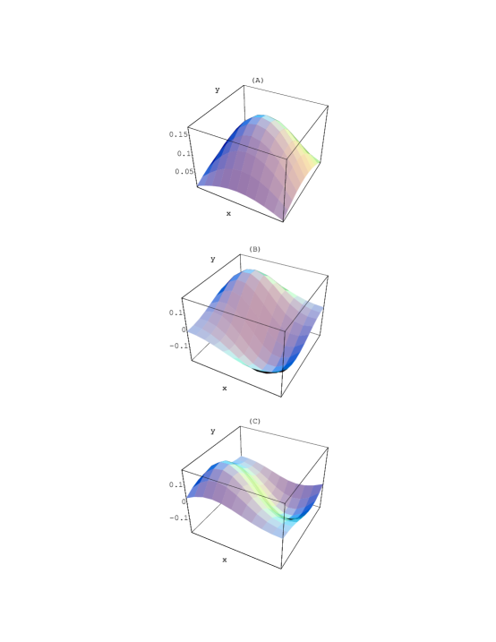
Figure 2: Eigenfunctions of first three states for the case of no doubling. n=5

For a zero transverse momentum fermion, the probability amplitude to be at any transverse location should be independent of the transverse location. Thus we expect the eigenfunction for such a particle to be a constant. At finite volume, with fixed boundary condition, we do get a nodeless wave function which nevertheless is not a constant since it carries some non-zero transverse momentum. All the excited states carry non-zero transverse momentum in the infinite volume limit. All of them have nodes characteristic of sine waves. The eigenfunctions corresponding to the first three eigenvalues are shown in Fig. 2 for the case of fixed boundary condition. With periodic boundary condition, for any $n$, we get a zero transverse momentum fermion with a flat wave function.

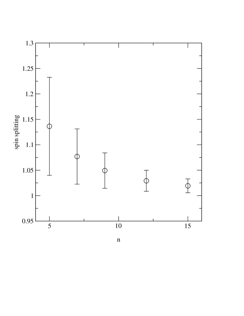
Figure 3: Spin splitting of the ground state caused by the spin dependent interaction as a function of n.

Now, we consider the effect of helicity flip term. With fixed boundary condition the lowest eigenstate has non vanishing transverse momentum in finite volume. In the absence of helicity flip term positive and negative helicity fermions are degenerate. The helicity flip term lifts the degeneracy. The splitting is larger for larger transverse momentum. In Fig. 3 we present the level splitting for the helicity up and down fermions as a function of $n$. As expected, the level splitting vanishes and we get exact degeneracy in the infinite volume limit. For the periodic boundary condition, the lowest state has exactly zero transverse momentum and we get two degenerate fermions for all $n$.

IV Hamiltonian with symmetric derivative

IV.1 construction

The symmetric derivative is defined by

$$D_{r}\psi^{\pm}({\bf x})={1\over 2a}[U_{r}({\bf x})\psi^{\pm}({\bf x}+a{\hat{\bf r}})-U_{-r}({\bf x})\psi^{\pm}({\bf x}-a{\hat{\bf r}})].$$ (31)

In place of using forward and backward derivatives in Eq. (14), we use the above symmetric derivative for all lattice derivatives. Proceeding as in Sec. IIIA, we arrive at the fermionic part of the QCD Hamiltonian

$$P^{-}_{sd} = \int dx^{-}a^{2}\sum_{\bf x}m^{2}\eta^{\dagger}({\bf x}){1\over i\partial^{+}}\eta({\bf x})$$ (32)

$$-\int dx^{-}a^{2}\sum_{\bf x}\Bigg{\{}m\frac{1}{2a}\eta^{\dagger}({\bf x})\sum_{r}{\hat{\sigma}}_{r}{1\over i\partial^{+}}\left[U_{r}({\bf x})\eta({\bf x}+a{\hat{\bf r}})-U_{-r}({\bf x})\eta({\bf x}-a{\hat{\bf r}})\right]$$

$$-m\frac{1}{2a}\sum_{r}\left[\eta^{\dagger}({\bf x}-a{\hat{\bf r}}){\hat{\sigma}}_{r}U_{r}({\bf x}-a{\hat{\bf r}})-\eta^{\dagger}({\bf x}+a{\hat{\bf r}}){\hat{\sigma}}_{r}U_{-r}({\bf x}+a{\hat{\bf r}})\right]{1\over i\partial^{+}}\eta({\bf x})\Bigg{\}}$$

$$-\int dx^{-}a^{2}\sum_{\bf x}\frac{1}{4a^{2}}\sum_{r}\Big{[}\eta^{\dagger}({\bf x}-a{\hat{\bf r}})U_{r}({\bf x}-a{\hat{\bf r}})-\eta^{\dagger}({\bf x}+a{\hat{\bf r}})U_{-r}({\bf x}+a{\hat{\bf r}})\Big{]}$$

$$~{}~{}~{}~{}~{}{1\over i\partial^{+}}\Big{[}U_{r}({\bf x})\eta({\bf x}+a{\hat{\bf r}})-U_{-r}({\bf x})\eta({\bf x}-a{\hat{\bf r}})\Big{]}.$$

In the free limit, the above Hamiltonian becomes

$$P^{-}_{sd} = \int dx^{-}a^{2}\sum_{\bf x}\Bigg{\{}m^{2}{\eta}^{\dagger}({\bf x}){1\over i\partial^{+}}\eta({\bf x})$$ (33)

$$+{1\over 4a^{2}}\sum_{r}[{\eta}^{\dagger}({\bf x}+a{\hat{\bf r}})-{\eta}^{\dagger}({\bf x}-a{\hat{\bf r}})]{1\over i\partial^{+}}[\eta({\bf x}+a{\hat{\bf r}})-\eta({\bf x}-a{\hat{\bf r}})]\Bigg{\}}.$$

In the free field limit the two linear mass terms cancel with each other.

Using DLCQ for the longitudinal direction, we get

$$P_{sd}^{-}={L\over\pi}H_{sd}\equiv{L\over\pi}[H_{m}+H_{k}]$$ (34)

with

$$H_{m} = a^{2}{m}^{2}\sum_{l}\sum_{\sigma}\sum_{\bf z}{1\over l}$$ (35)

$$~{}~{}~{}~{}[b^{\dagger}(l,{\bf z},\sigma)b(l,{\bf z},\sigma)+d^{\dagger}(l,{\bf z},\sigma)d(l,{\bf z},\sigma)]$$

and

$$H_{k} = \sum_{l}\sum_{\sigma}\sum_{\bf z}\sum_{r}{1\over l}$$ (36)

$$~{}~{}~{}\Bigg{[}b^{\dagger}(l,{\bf z}+a{\hat{\bf r}},\sigma)b(l,{\bf z}+a{\hat{\bf r}},\sigma)+b^{\dagger}(l,{\bf z}-a{\hat{\bf r}},\sigma)b(l,{\bf z}-a{\hat{\bf r}},\sigma)$$

$$~{}~{}~{}-b^{\dagger}(l,{\bf z}+a{\hat{\bf r}},\sigma)b(l,{\bf z}-a{\hat{\bf r}},\sigma)-b^{\dagger}(l,{\bf z}-a{\hat{\bf r}},\sigma)b(l,{\bf z}+a{\hat{\bf r}},\sigma)$$

$$~{}~{}~{}+d^{\dagger}(l,{\bf z}+a{\hat{\bf r}},\sigma)d(l,{\bf z}+a{\hat{\bf r}},\sigma)+d^{\dagger}(l,{\bf z}-a{\hat{\bf r}},\sigma)d(l,{\bf z}-a{\hat{\bf r}},\sigma)$$

$$~{}~{}~{}-d^{\dagger}(l,{\bf z}+a{\hat{\bf r}},\sigma)d(l,{\bf z}-a{\hat{\bf r}},\sigma)-d^{\dagger}(l,{\bf z}-a{\hat{\bf r}},\sigma)d(l,{\bf z}+a{\hat{\bf r}},\sigma)\Bigg{]}.$$

When we implement the constraint equation on the lattice and use symmetric definition of the lattice derivative, it is important to keep in mind that we have only next to nearest neighbor interactions. Thus a decoupling of even and odd lattice points occur and as a result we have two independent sub-lattices one connecting odd lattice points and the other connecting even lattice points.

Let us now address the nature of the spectrum and the presence of doublers.

IV.2 Fermion doubling

The Hamiltonian (33) can be rewritten as

$$P^{-}_{sd} = \int dx^{-}a^{2}\sum_{{\bf x}=even}\Big{[}m^{2}\eta^{\dagger}({\bf x}){1\over i\partial^{+}}\eta({\bf x})-{1\over 4a^{2}}a^{2}[\eta^{\dagger}({\bf x}){1\over i\partial^{+}}\sum_{r}[\eta({\bf x}+2a{\hat{\bf r}})]+\eta({\bf x}-2a{\hat{\bf r}})-2\eta({\bf x})]\Big{]}$$ (37)

$$+\int dx^{-}a^{2}\sum_{{\bf x}=odd}\Big{[}m^{2}\eta^{\dagger}({\bf x}){1\over i\partial^{+}}\eta({\bf x})-{1\over 4a^{2}}a^{2}[\eta^{\dagger}({\bf x}){1\over i\partial^{+}}\sum_{r}[\eta({\bf x}+2a{\hat{\bf r}})]+\eta({\bf x}-2a{\hat{\bf r}})-2\eta({\bf x})]\Big{]}.$$

Clearly the Hamiltonian is divided into even and odd sub-lattices each with lattice constant $2a$. As a result, a momentum component in each sub-lattice is bounded by ${\pi\over 2a}$ in magnitude. Again, going through the Fourier transform in each sub-lattice of the transverse space, we arrive at the free particle dispersion relation for the light front energy in each sector

$$k^{-}_{\bf k}={1\over k^{+}}[m^{2}+{1\over a^{2}}\sum_{r}\sin^{2}~{}k_{r}a].$$ (38)

For fixed $k_{r}$, in the limit $a\rightarrow 0$ ${1\over a^{2}}\sin^{2}~{}k_{r}a\rightarrow k_{r}^{2}$ and we get the continuum dispersion relation

$$k^{-}_{\bf k}={m^{2}+{\bf k}^{2}\over k^{+}}.$$ (39)

Because of the momentum bound of ${\pi\over 2a}$ doublers cannot arise from $ka=\pi$. However, because of the decoupling of odd and even lattices, one can get two zero transverse momentum fermions one each from the two sub-lattices. Thus, for two transverse dimensions, we can get four zero transverse momentum fermions as follows: (1) even lattice points in $x$, even lattice points in $y$, (2) even lattice points in $x$, odd lattice points in $y$, (3) odd lattice points in $x$, even lattice points in $y$, and (4) odd lattice points in $x$, odd lattice points in $y$. Thus we expect a four fold degeneracy of zero transverse momentum fermions.

IV.3 Numerical Investigation

IV.3.1 Fixed boundary condition

For each transverse direction, we have $2n+1$ lattice points where the fermions are allowed to hop. To implement the fixed boundary condition, we need to consider $2n+5$ lattice points. For one sub-lattice we have to fix particles at $s=1$ and $s=2n+5$. We have, the wavefunction at location $s$, $u_{s}\sim\sin~{}(s-1)ka$. We have, $u_{s}=0$ for $s=1$. We also need $u_{s}=0$ for $s=2n+5$. Thus $(2n+4)k_{p}a=p\pi$, with $p=1,2,3,...,n+1$. For $n=1$, allowed values of $k_{p}$ are $k_{p}={\pi\over 6a},{2\pi\over 6a}$.

For the other sub-lattice, we fix the particles at $s=2$ and $s=2n+4$. The wavefunction at location $s$, $u_{s}\sim\sin~{}(s-2)ka$. $u_{s}=0$ for $s=2$ and $s=2n+4$. Thus $(2n+2)k_{p}a=p\pi$ with $p=1,2,3,....,n$. For $n=1$, only allowed value of $k$ is $k={\pi\over 4a}$.

Combining the two sub-lattices, for $n=1$, the allowed values of $k$ are ${\pi\over 6a},{\pi\over 4a},$ and ${2\pi\over 6a}$.

IV.3.2 Periodic boundary condition

For a given $n$, fermions are allowed to hop at $2n+1$ lattice points in each transverse directions. Consider $2n+3$ lattice points. For one sub-lattice $(2n+3)^{rd}$ lattice point is identified with the lattice point 1. For the other sub-lattice $(2n+2)^{nd}$ lattice point is identified with the lattice point 2. Wavefunction at point $s$, $u_{s}\sim e^{iska}$. We require $e^{ika}=e^{i(2n+3)ka}$. Thus $k_{p}a=\pm{2\pi p\over(2n+2)}$, $p=0,1,2,...,{n+1\over 2}$. For $n=1$, we have, $k_{0}=0,k_{1}=\pm{\pi\over 2a}$.

For the other sub-lattice we require $e^{2ika}=e^{i(2n+2)ka}$. Thus $k_{p}a=\pm{\pi\over n}p$, $p=0,1,2,...,{n-1\over 2}$. For $n=1$, allowed value of $k=0$. Thus for $n=1$, taking the two sub-lattices together, the allowed values of $k$ are $0,0,{\pi\over 2a}$.

IV.3.3 Numerical results

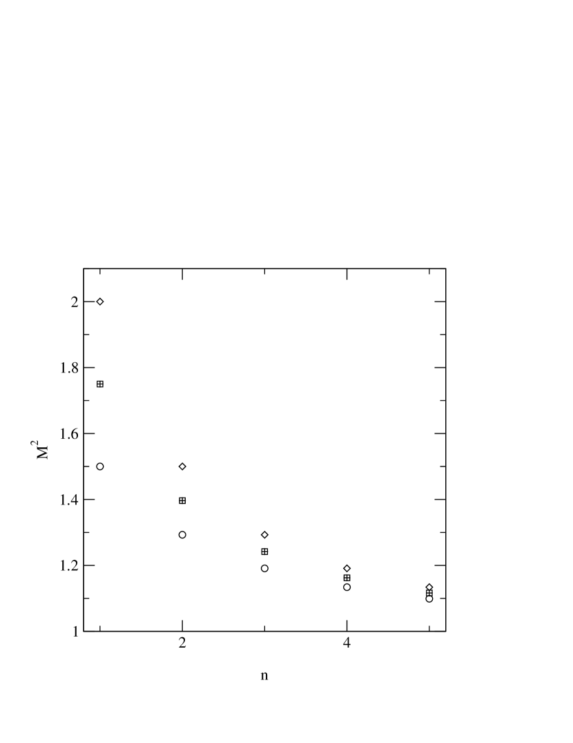
Figure 4: First four eigenvalues as a function of n.

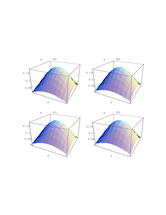
Figure 5: Eigenfunctions of first four (degenerate) states for the case of fermion doubling. n=5

The results of matrix diagonalization in the case of the symmetric derivative with fixed boundary condition are presented in Figs. 4, 5 and 6. In Fig. 4 we present the lowest four eigenvalues as a function of $n$. At finite volume, the four states do not appear exactly degenerate even though the even-odd and odd-even states are always degenerate because of the hypercubic (square) symmetry in the transverse plane. The four states become degenerate in the infinite volume limit. The eigenfunctions of the lowest four states are presented in Fig. 5 for $n=5$. As they correspond to particle states, they are nodeless. All other states in the spectrum have one or more nodes. For example, in Fig. 6 we show the eigenfunction corresponding to the fifth eigenvalue which clearly exhibits the node structure.

With periodic boundary condition, for any $n$ we get four degenerate eigenvalues corresponding to zero transverse momentum fermions. Corresponding wavefunctions are flat in transverse coordinate space.

V Staggered fermion on the light front transverse lattice

As we have seen in the previous section that the method of symmetric derivatives results in fermion doublers, we now consider two approaches to remove the doublers. In this section we study an approach similar to the staggered fermions in conventional lattice gauge theory. In the next section we will take up the case of Wilson fermions.

In analogy with the Euclidean staggered formulation, define the spin diagonalization transformation

$$\eta(x_{1},x_{2})=({\hat{\sigma}}^{1})^{x_{1}}({\hat{\sigma}}^{2})^{x_{2}}\chi(x_{1},x_{2}).$$ (40)

We see from the QCD Hamiltonian given in Eq. (32) with symmetric derivative that in the interacting theory (except for the linear mass term) and also in the free fermion limit, even and odd lattice sites are decoupled and the Hamiltonian is already spin diagonal. So, it is very natural to try staggered fermion formulation on the light front transverse lattice. In this section we shall follow the Kogut-Susskind formulation ks and present an elementary configuration space analysis for two flavor interpretation. After the spin transformation the linear mass term in the Hamiltonian (32) becomes:

$$\int dx^{-}a^{2}\sum_{\bf x}\Bigg{\{}m\frac{1}{2a}\chi^{\dagger}({\bf x})\sum_{r}\phi({\bf x},r){1\over i\partial^{+}}\left[U_{r}({\bf x})\chi({\bf x}+a{\hat{\bf r}})-U_{-r}({\bf x})\chi({\bf x}-a{\hat{\bf r}})\right]$$ (41)

$$-m\frac{1}{2a}\sum_{r}\left[\chi^{\dagger}({\bf x}-a{\hat{\bf r}})\phi({\bf x},r)U_{r}({\bf x}-a{\hat{\bf r}})-\chi^{\dagger}({\bf x}+a{\hat{\bf r}})\phi({\bf x},r)U_{-r}({\bf x}+a{\hat{\bf r}})\right]{1\over i\partial^{+}}\chi({\bf x})\Bigg{\}}$$

where, $\phi({\bf x},r)=1$ for $r=1$ and $\phi({\bf x},r)=(-1)^{x_{1}}$ for $r=2$. After spin diagonalization, the full Hamiltonian in the free field limit becomes

$$P^{-}_{sf} = \int dx^{-}a^{2}\sum_{\bf x}\Bigg{\{}m^{2}{\chi}^{\dagger}({\bf x}){1\over i\partial^{+}}\chi({\bf x})$$ (42)

$$+{1\over 4a^{2}}\sum_{r}[{\chi}^{\dagger}({\bf x}+a{\hat{\bf r}})-{\chi}^{\dagger}({\bf x}-a{\hat{\bf r}})]{1\over i\partial^{+}}[\chi({\bf x}+a{\hat{\bf r}})-\chi({\bf x}-a{\hat{\bf r}})]$$

$$-{1\over 2a}m{\chi}^{\dagger}({\bf x}){1\over i\partial^{+}}\sum_{r}\phi({\bf x},r)[\chi({\bf x}+a{\hat{\bf r}})-\chi({\bf x}-a{\hat{\bf r}})]$$

$$-{1\over 2a}m\sum_{r}[{\chi}^{\dagger}({\bf x}+a{\hat{\bf r}})-{\chi}^{\dagger}({\bf x}-a{\hat{\bf r}})]\phi({\bf x},r){1\over i\partial^{+}}\chi({\bf x})\Bigg{\}}.$$

The two linear mass terms cancel with each other in the free theory, but since they are present in the interacting theory we keep them to investigate the staggered fermions.

Since all the terms in Eq. (42) are spin diagonal, we can put only a single component field at each transverse site. From now on, all the $\chi$’s and $\chi^{\dagger}$’s appearing in Eq. (42) can be taken as single component fermion fields. Thus we have thinned the fermionic degrees of freedom by half. Without loss of generality, we keep the helicity up component of $\chi$ at each lattice point.

Apart from the linear mass term in Eq. (42), all the other terms have the feature that fermion fields on the even and odd lattices do not mix. Let us denote (see Fig. 7) the even-even lattice points by 1, odd-odd lattice points by $1^{\prime}$, odd-even lattice points by 2 and even-odd lattice points by $2^{\prime}$, and the corresponding fields by $\chi_{1}$ etc. Then the first of the linear mass terms

$$\sum_{{\bf x}}{\chi}^{\dagger}({\bf x}){1\over i\partial^{+}}\sum_{r}\phi({\bf x},r)[\chi({\bf x}+a{\hat{\bf r}})-\chi({\bf x}-a{\hat{\bf r}})]$$ (43)

can be rewritten as (suppressing factors of $a$),

$${\chi_{1}}^{\dagger}{1\over i\partial^{+}}(\nabla_{1}\chi_{2}+\nabla_{2}\chi_{2^{\prime}})+{\chi_{2}}^{\dagger}{1\over i\partial^{+}}(\nabla_{1}\chi_{1}-\nabla_{2}\chi_{1^{\prime}})$$ (44)

$$+{\chi_{1^{\prime}}}^{\dagger}{1\over i\partial^{+}}(\nabla_{1}\chi_{2^{\prime}}-\nabla_{2}\chi_{2})+{\chi_{2^{\prime}}}^{\dagger}{1\over i\partial^{+}}(\nabla_{1}\chi_{1^{\prime}}+\nabla_{2}\chi_{1})+B$$

where $\nabla_{1}$ and $\nabla_{2}$ are the symmetric derivatives in the respective directions. Looking at Fig. 7 it is apparent that these $\nabla_{1}$ and $\nabla_{2}$ can also be interpreted as a block derivative, i.e., finite differences between block variables. For example, $\nabla_{1}\chi_{1}=\chi_{1}(1,0)-\chi_{1}(0,0)$. $B$ represents the contribution from other blocks.

Using Eq. (40), in terms of the nonvanishing components of $\eta$, we have

$$\eta_{1}=\chi_{1},~{}~{}\eta_{2}=i\chi_{2},~{}~{}\eta_{1^{\prime}}=i\chi_{1^{\prime}},~{}~{}\eta_{2^{\prime}}=-\chi_{2^{\prime}}.$$ (45)

An interesting feature of lattice points 1 and $1^{\prime}$ is that fermion fields $\eta_{1}$ and $\eta_{1^{\prime}}$ have positive helicity. $\eta_{2}$ and $\eta_{2^{\prime}}$ have negative helicity. In terms of $\eta$ fields the expression given in Eq. (44) can be written as

$${\eta_{1}}^{\dagger}{1\over i\partial^{+}}(-i\nabla_{1}\eta_{2}-\nabla_{2}\eta_{2^{\prime}})+i{\eta_{2}}^{\dagger}{1\over i\partial^{+}}(\nabla_{1}\eta_{1}+i\nabla_{2}\eta_{1^{\prime}})$$ (46)

$$+i{\eta_{1^{\prime}}}^{\dagger}{1\over i\partial^{+}}(-\nabla_{1}\eta_{2^{\prime}}+i\nabla_{2}\eta_{2})-{\eta_{2^{\prime}}}^{\dagger}{1\over i\partial^{+}}(-i\nabla_{1}\eta_{1^{\prime}}+\nabla_{2}\eta_{1})+B.$$

Now,

$$\eta(1)-\eta(0) = {1\over 2}(\eta(1)-\eta(-1))+{1\over 2}(\eta(1)+\eta(-1)-2\eta(0))$$ (47)

$$\equiv {\hat{\nabla}}\eta(0)+{1\over 2}{\hat{\nabla}}^{2}\eta(0)~{},$$

$$\eta(0)-\eta(-1) = {1\over 2}(\eta(1)-\eta(-1))-{1\over 2}(\eta(1)+\eta(-1)-2\eta(0))$$ (48)

$$\equiv {\hat{\nabla}}\eta(0)-{1\over 2}{\hat{\nabla}}^{2}\eta(0)$$

where ${\hat{\nabla}}$ and ${\hat{\nabla}}^{2}$ are respectively first order and second order block derivatives. So, we can write the expression (46) as

$${\eta_{1}}^{\dagger}{1\over i\partial^{+}}\Big{\{}-i({\hat{\nabla}}_{1}\eta_{2}-{1\over 2}{{\hat{\nabla}}_{1}}^{2}\eta_{2})-({\hat{\nabla}}_{2}\eta_{2^{\prime}}-{1\over 2}{{\hat{\nabla}}_{2}}^{2}\eta_{2^{\prime}}\Big{\}}$$ (49)

$$+i{\eta_{2}}^{\dagger}{1\over i\partial^{+}}\Big{\{}({\hat{\nabla}}_{1}\eta_{1}+{1\over 2}{{\hat{\nabla}}_{1}}^{2}\eta_{1})+i({\hat{\nabla}}_{2}\eta_{1^{\prime}}-{1\over 2}{{\hat{\nabla}}_{2}}^{2}\eta_{1^{\prime}})\Big{\}}$$

$$+i{\eta_{1^{\prime}}}^{\dagger}{1\over i\partial^{+}}\Big{\{}-({\hat{\nabla}}_{1}\eta_{2^{\prime}}+{1\over 2}{{\hat{\nabla}}_{1}}^{2}\eta_{2^{\prime}})+i({\hat{\nabla}}_{2}\eta_{2}+{1\over 2}{{\hat{\nabla}}_{2}}^{2}\eta_{2})\Big{\}}$$

$$-{\eta_{2^{\prime}}}^{\dagger}{1\over i\partial^{+}}\Big{\{}-i({\hat{\nabla}}_{1}\eta_{1^{\prime}}-{1\over 2}{{\hat{\nabla}}_{1}}^{2}\eta_{1^{\prime}})+({\hat{\nabla}}_{2}\eta_{1}+{1\over 2}{{\hat{\nabla}}_{2}}^{2}\eta_{1})\Big{\}}~{}.$$

Let us introduce the fields

$$u_{1} = {1\over{\sqrt{2}}}(\eta_{1}+\eta_{1^{\prime}})$$

$$u_{2} = {1\over{\sqrt{2}}}(\eta_{2}+\eta_{2^{\prime}})$$

$$\tilde{d}_{1} = {1\over{\sqrt{2}}}(\eta_{1}-\eta_{1^{\prime}})$$

$$\tilde{d}_{2} = {1\over{\sqrt{2}}}(\eta_{2}-\eta_{2^{\prime}}).$$

Then, the first order derivative term in Eq. (49) can be written as

$$u^{\dagger}{1\over i\partial^{+}}{\hat{\sigma}}^{r}{\hat{\nabla}}_{r}u+d^{\dagger}{1\over i\partial^{+}}{\hat{\sigma}}^{r}{\hat{\nabla}}_{r}d=f^{\dagger}{1\over i\partial^{+}}{\hat{\sigma}}^{r}{\hat{\nabla}}_{r}f$$ (51)

where, $d={\hat{\sigma}}^{1}\tilde{d}$ and the flavor isospin doublet

$$f=\left[\begin{array}[]{l}u\\ d\end{array}\right].$$ (54)

Similarly, we can write the second order block derivative term in expression (49) as

$${1\over 2}f^{\dagger}{1\over i\partial^{+}}\sigma^{3}{T}^{r}{{\hat{\nabla}}_{r}}^{2}f$$ (55)

where, $T^{r}$s are the matrices in the flavor space defined as

$$T^{1}=-i\sigma^{2},~{}~{}~{}T^{2}=-i\sigma^{1}.$$ (56)

Similarly, the second term in Eq. (42)

$$\sum_{r}[{\eta}^{\dagger}({\bf x}+a{\hat{\bf r}})-{\eta}^{\dagger}({\bf x}-a{\hat{\bf r}})]{1\over i\partial^{+}}[\eta({\bf x}+a{\hat{\bf r}})-\eta({\bf x}-a{\hat{\bf r}})]$$ (57)

reads as

$${\hat{\nabla}}_{r}f^{\dagger}{1\over i\partial^{+}}{\hat{\nabla}}_{r}f+{{\hat{\nabla}}_{r}}^{2}f^{\dagger}{1\over i\partial^{+}}{{\hat{\nabla}}_{r}}^{2}f+{i\over 2}[{\hat{\nabla}}_{r}f^{\dagger}{1\over i\partial^{+}}\sigma^{r}T^{r}{{\hat{\nabla}}_{r}}^{2}f+{{\hat{\nabla}}_{r}}^{2}f^{\dagger}{1\over i\partial^{+}}\sigma^{r}T^{r}{{\hat{\nabla}}_{r}}f]~{}.$$ (58)

The full Hamiltonian given in Eq. (42) can now be written in two flavor notation as

$$P^{-}_{sf}=\int dx^{-}a^{2}\sum_{x} \Big{\{} m^{2}f^{\dagger}{1\over i\partial^{+}}f+{1\over 4}[{\hat{\nabla}}_{r}f^{\dagger}{1\over i\partial^{+}}{\hat{\nabla}}_{r}f+a^{2}{{\hat{\nabla}}_{r}}^{2}f^{\dagger}{1\over i\partial^{+}}{{\hat{\nabla}}_{r}}^{2}f$$ (59)

$$+{ia\over 2}({\hat{\nabla}}_{r}f^{\dagger}{1\over i\partial^{+}}\sigma^{r}T^{r}{{\hat{\nabla}}_{r}}^{2}f+{{\hat{\nabla}}_{r}}^{2}f^{\dagger}{1\over i\partial^{+}}\sigma^{r}T^{r}{{\hat{\nabla}}_{r}}f)]$$

$$-{1\over 2}m(f^{\dagger}{1\over i\partial^{+}}{\hat{\sigma}}^{r}{\hat{\nabla}}_{r}f+{a\over 2}f^{\dagger}{1\over i\partial^{+}}\sigma^{3}{T}^{r}{{\hat{\nabla}}_{r}}^{2}f+h.c)\Big{\}}~{}.$$

The above simple exercise shows that applying the spin diagonalization on the symmetric derivative method, the number of doublers on the transverse lattice can be reduced from four to two which can be reinterpreted as two flavors. Although in the free case given by Eq. (59) the second and third lines are separately zero identically, we have kept these terms because in QCD similar terms will survive. These terms exhibit flavor mixing and also helicity flipping. The flavor mixing terms are always irrelevant.

VI Wilson term on the light front transverse lattice

Since doublers in the light front transverse lattice arise from the decoupling of even and odd lattice sites, a term that will couple these sites will remove the zero momentum doublers. However, conventional doublers now may arise from the edges of the Brillouin zone. A second derivative term couples the even and odd lattice sites and also removes the conventional doublers. Thus, the term originally proposed by Wilson to remove the doublers arising from $ka=\pi$ in the conventional lattice theory will do the job BK .

To remove doublers, add an irrelevant term to the Lagrangian density

$$\delta{\cal L}({\bf x})={\kappa\over a}\sum_{r}{\bar{\psi}}({\bf x})[U_{r}({\bf x})\psi({\bf x}+a{\hat{\bf r}})-2\psi({\bf x})+U_{-r}({\bf x})\psi({\bf x}-a{\hat{\bf r}})]$$ (60)

where $\kappa$ is the Wilson parameter. This generates the following additional terms in the Hamiltonian (32):

$$P^{-}_{w} = -\int dx^{-}a^{2}\sum_{\bf x}\Bigg{\{}4\frac{\kappa}{a}\frac{1}{2a}\eta^{\dagger}({\bf x})\sum_{r}{\hat{\sigma}}_{r}{1\over i\partial^{+}}\left[U_{r}({\bf x})\eta({\bf x}+a{\hat{\bf r}})-U_{-r}({\bf x})\eta({\bf x}-a{\hat{\bf r}})\right]$$ (61)

$$-4\frac{\kappa}{a}\frac{1}{2a}\sum_{r}\left[\eta^{\dagger}({\bf x}-a{\hat{\bf r}}){\hat{\sigma}}_{r}U_{r}({\bf x}-a{\hat{\bf r}})-\eta^{\dagger}({\bf x}+a{\hat{\bf r}}){\hat{\sigma}}_{r}U_{-r}({\bf x}+a{\hat{\bf r}})\right]{1\over i\partial^{+}}\eta({\bf x})\Bigg{\}}$$

$$+\int dx^{-}a^{2}\sum_{\bf x}\Bigg{\{}\frac{\kappa}{a}\frac{1}{2a}\sum_{r}\sum_{s}\Big{[}\eta^{\dagger}({\bf x}-a{\hat{\bf r}})U_{r}({\bf x}-a{\hat{\bf r}})+\eta^{\dagger}({\bf x}+a{\hat{\bf r}})U_{-r}({\bf x}+a{\hat{\bf r}})\Big{]}$$

$$~{}~{}~{}~{}~{}{1\over i\partial^{+}}{\hat{\sigma}}_{s}\Big{[}U_{s}({\bf x})\eta({\bf x}+a{\hat{\bf s}})-U_{-s}({\bf x})\eta({\bf x}-a{\hat{\bf s}})\Big{]}$$

$$-\frac{\kappa}{a}\frac{1}{2a}\sum_{r}\sum_{s}\Big{[}\eta^{\dagger}({\bf x}-a{\hat{\bf r}}){\hat{\sigma}}_{r}U_{r}({\bf x}-a{\hat{\bf r}})-\eta^{\dagger}({\bf x}+a{\hat{\bf r}}){\hat{\sigma}}_{r}U_{-r}({\bf x}+a{\hat{\bf r}})\Big{]}$$

$$~{}~{}~{}~{}~{}{1\over i\partial^{+}}\Big{[}U_{s}({\bf x})\eta({\bf x}+a{\hat{\bf s}})+U_{-s}({\bf x})\eta({\bf x}-a{\hat{\bf s}})\Big{]}\Bigg{\}}$$

$$-\int dx^{-}a^{2}\sum_{\bf x}\Bigg{\{}\mu\frac{\kappa}{a}\eta^{\dagger}({\bf x}){1\over i\partial^{+}}\sum_{r}\left[U_{r}({\bf x})\eta({\bf x}+a{\hat{\bf r}})+U_{-r}({\bf x})\eta({\bf x}-a{\hat{\bf r}})\right]$$

$$+\mu\frac{\kappa}{a}\sum_{r}\left[\eta^{\dagger}({\bf x}-a{\hat{\bf r}})U_{r}({\bf x}-a{\hat{\bf r}})+\eta^{\dagger}({\bf x}+a{\hat{\bf r}})U_{-r}({\bf x}+a{\hat{\bf r}})\right]{1\over i\partial^{+}}\eta({\bf x})\Bigg{\}}$$

$$-\int dx^{-}a^{2}\sum_{\bf x}\frac{\kappa^{2}}{a^{2}}\sum_{r}\sum_{s}\Big{[}\eta^{\dagger}({\bf x}-a{\hat{\bf r}})U_{r}({\bf x}-a{\hat{\bf r}})+\eta^{\dagger}({\bf x}+a{\hat{\bf r}})U_{-r}({\bf x}+a{\hat{\bf r}})\Big{]}$$

$$~{}~{}~{}~{}~{}{1\over i\partial^{+}}\Big{[}U_{s}({\bf x})\eta({\bf x}+a{\hat{\bf s}})+U_{-s}({\bf x})\eta({\bf x}-a{\hat{\bf s}})\Big{]}.$$

In addition, the factor $m^{2}$ in the free term in (32) gets replaced by $\mu^{2}=(m+4{\kappa\over a})^{2}$.

In the free limit the resulting Hamiltonian goes over to

$$P^{-}_{w} = \int dx^{-}a^{2}\sum_{{\bf x}}\Bigg{[}\mu^{2}{\eta}^{\dagger}({\bf x}){1\over i\partial^{+}}\eta({\bf x})$$ (62)

$$+{1\over 2a}\sum_{r}[{\eta}^{\dagger}({\bf x}+a{\hat{\bf r}})-{\eta}^{\dagger}({\bf x}-a{\hat{\bf r}})]{1\over i\partial^{+}}{1\over 2a}[\eta({\bf x}+a{\hat{\bf r}})-\eta({\bf x}-a{\hat{\bf r}})]$$

$$+{\kappa^{2}\over a^{2}}\sum_{r}[{\eta}^{\dagger}({\bf x}+a{\hat{\bf r}})-2{\eta}^{\dagger}({\bf x})+{\eta}^{\dagger}({\bf x}-a{\hat{\bf r}})]{1\over i\partial^{+}}[\eta({\bf x}+a{\hat{\bf r}})-2\eta({\bf x})+\eta({\bf x}-a{\hat{\bf r}})]$$

$$-2{\mu\kappa\over a}\sum_{r}{\eta}^{\dagger}({\bf x}){1\over i\partial^{+}}[\eta({\bf x}+a{\hat{\bf r}})-2\eta({\bf x})+\eta({\bf x}-a{\hat{\bf r}})]\Bigg{]}.$$

We rewrite the free Hamiltonian (62) as

$$P_{w}^{-}=P_{D}^{-}+P_{OD1}^{-}+P_{OD2}^{-}.$$ (63)

The diagonal terms are

$$P^{-}_{D} = \int dx^{-}a^{2}\sum_{{\bf x}}{\eta}^{\dagger}({\bf x}){1\over i\partial^{+}}\eta({\bf x})\Big{[}\mu^{2}+{1\over a^{2}}+8\mu\kappa{1\over a}+12\kappa^{2}{1\over a^{2}}\Big{]}.$$ (64)

The nearest neighbor interaction is

$$P^{-}_{OD1} = -\int dx^{-}a^{2}\sum_{{\bf x}}\sum_{{\hat{\bf r}}}$$ (65)

$$\Bigg{[}(2\mu\kappa{1\over a}+4{\kappa^{2}\over a^{2}})\Big{[}{\eta}^{\dagger}({\bf x}){1\over i\partial^{+}}\eta({\bf x}+a{\hat{\bf r}})+{\eta}^{\dagger}({\bf x}){1\over i\partial^{+}}\eta({\bf x}+a{\hat{\bf r}})\Big{]}\Bigg{]}.$$

The next to nearest neighbor interaction is

$$P^{-}_{OD2} = \int dx^{-}a^{2}\sum_{{\bf x}}\sum_{{\hat{\bf r}}}\Big{\{}-{1\over 4a^{2}}+{\kappa^{2}\over a^{2}}\Big{\}}$$

$$\Big{[}{\eta}^{\dagger}({\bf x}+a{\hat{\bf r}}){1\over i\partial^{+}}\eta({\bf x}-a{\hat{\bf r}})+{\eta}^{\dagger}({\bf x}-a{\hat{\bf r}}){1\over i\partial^{+}}\eta({\bf x}+a{\hat{\bf r}})\Big{]}.$$

Using the Fourier transform in the transverse space, we get,

$$P^{-}_{w} = \int dx^{-}\int{d^{2}k\over(2\pi)^{2})}\phi_{\bf k}^{\dagger}(x^{-}){1\over i\partial^{+}}\phi_{\bf k}(x^{-})\Bigg{[}\mu^{2}+\sum_{r}k_{r}^{2}\Bigg{(}{\sin k_{r}a\over k_{r}a}\Bigg{)}^{2}$$ (67)

$$+2a\mu\kappa\sum_{r}k_{r}^{2}\Bigg{(}{\sin k_{r}a/2\over k_{r}a/2}\Bigg{)}^{2}~{}+a^{2}\kappa^{2}\sum_{r}k_{r}^{4}\Bigg{(}{\sin k_{r}a/2\over k_{r}a/2}\Bigg{)}^{4}~{}\Bigg{]}.$$

Note that, as anticipated, Wilson term removes the doublers because the lowest eigenvalue occurs only if all the $k_{r}$’s are zero.

In DLCQ, we have,

$$H_{D} = [a^{2}{\mu}^{2}+1+8a\mu\kappa+12\kappa^{2}]\sum_{l}\sum_{\sigma}\sum_{\bf z}{1\over l}$$ (68)

$$~{}~{}~{}~{}[b^{\dagger}(l,{\bf z},\sigma)b(l,{\bf z},\sigma)+d^{\dagger}(l,{\bf z},\sigma)d(l,{\bf z},\sigma)],$$

$$H_{OD1} = -[2\kappa a\mu+4\kappa^{2}]\sum_{l}\sum_{\sigma}\sum_{\bf z}\sum_{r}{1\over l}$$ (69)

$$~{}~{}~{}\Bigg{[}b^{\dagger}(l,{\bf z},\sigma)b(l,{\bf z}+a{\hat{\bf r}},\sigma)+b^{\dagger}(l,{\bf z},\sigma)b(l,{\bf z}-a{\hat{\bf r}},\sigma)$$

$$~{}~{}~{}+d^{\dagger}(l,{\bf z},\sigma)d(l,{\bf z}+a{\hat{\bf r}},\sigma)+d^{\dagger}(l,{\bf z},\sigma)d(l,{\bf z}-a{\hat{\bf r}},\sigma)\Bigg{]}$$

and

$$H_{OD2} = -[{1\over 4}-\kappa^{2}]\sum_{l}\sum_{\sigma}\sum_{\bf z}\sum_{r}{1\over l}$$ (70)

$$~{}~{}~{}\Bigg{[}b^{\dagger}(l,{\bf z}+a{\hat{\bf r}},\sigma)b(l,{\bf z}-a{\hat{\bf r}},\sigma)+b^{\dagger}(l,{\bf z}-a{\hat{\bf r}},\sigma)b(l,{\bf z}+a{\hat{\bf r}},\sigma)$$

$$~{}~{}~{}+d^{\dagger}(l,{\bf z}+a{\hat{\bf r}},\sigma)d(l,{\bf z}-a{\hat{\bf r}},\sigma)+d^{\dagger}(l,{\bf z}-a{\hat{\bf r}},\sigma)d(l,{\bf z}+a{\hat{\bf r}},\sigma)\Bigg{]}~{}.$$

VI.1 Numerical Investigation

VI.1.1 Boundary condition

With the Wilson term added, we do not have decoupled sub-lattices. We have both nearest neighbor and next-to-nearest neighbor interactions. Since with fixed boundary condition, the lowest four eigenvalues are not exactly degenerate in finite volume, it is difficult to investigate the removal of degeneracy by the addition of Wilson term. With periodic boundary condition, for a lattice with $2n+1$ lattice points in each transverse direction, we identify the $(2n+2)^{th}$ lattice site with the first lattice site. Then for the Hamiltonian matrix we get the following additional contributions.

$$H=\pmatrix{.&.&.&.&...&.&.&NN&N\cr.&.&.&.&...&.&.&0&NN\cr.&.&.&.&....&.&.&.&.\cr...\cr...\cr.&.&.&.&....&.&.&.&.\cr NN&0&.&.&...&.&.&.&.\cr N&NN&.&.&...&.&.&.&.}$$ (71)

The matrix elements $NN=-{1\over 4}+\kappa^{2}$ and $N=-2a\mu\kappa-4\kappa^{2}$. For a given $n$, the allowed values of $k$ are $k_{p}=\pm{2\pi p\over 2n+1}$, $p=0,1,2,......$. Thus for $n=3$, we expect multiples of ${2\pi\over 7}$ apart from $0$. For $n=5$, apart from $0$, allowed values of $k$ are multiples of ${2\pi\over 11}$.

VI.1.2 Numerical results

Since the Wilson term connects even and odd lattices, the extra fermions that appear at zero transverse momentum are removed once Wilson term is added as we now have nearest and next to nearest neighbor interactions. For large $n$, we get the expected spectra but, numerical results suggest that the finite volume effect is larger for small $\kappa$ which is obvious because $\kappa$ is a mass-like parameter. For example, with periodic boundary condition, for $n=3$, for $\kappa=1.0,0.5,0.4$, we get the expected harmonics but not for $\kappa=0.1$. The situation is similar for $n=5$. For $n=10$, expected harmonics emerge even for $\kappa=0.1$ but not for $\kappa=0.01$.

VII Doubling and symmetries on the light front transverse lattice

Because of the constraint equation which is inconsistent with the equal time chiral transformation in the presence of massive fermions, we should distinguish between chiral symmetry in the equal time formalism and in the light front formalism. For example, the free massive light front Lagrangian involving only the dynamical degrees of freedom is invariant under $\gamma_{5}$ transformation. On the light front, helicity takes over the notion of chirality even in presence of fermion mass which can be understood in the following way.

In the two component representation hz in the light front formalism, let us look at the objects $\psi_{L}^{+}$ and $\psi_{R}^{+}$. We have

$$\psi^{+}(x)=\pmatrix{\eta(x)\cr 0\cr}$$ (72)

with

$$\eta(x)=\pmatrix{\eta_{1}(x)\cr\eta_{2}(x)\cr}$$ (73)

The projection operators are $P_{R}={1\over 2}(1+\gamma^{5})$ and $P_{L}={1\over 2}(1-\gamma^{5})$ with

$$\gamma^{5}=\pmatrix{\sigma^{3}&0\cr 0&-\sigma^{3}\cr}.$$ (74)

Then

$$\psi_{R}^{+}=P_{R}\psi^{+}=\pmatrix{\eta_{1}\cr 0\cr 0\cr 0}$$ (75)

and

$$\psi_{L}^{+}=P_{L}\psi^{+}=\pmatrix{0\cr\eta_{2}\cr 0\cr 0}.$$ (76)

Thus $\psi_{R}^{+}=P_{R}\psi^{+}$ represents a positive helicity fermion and $\psi_{L}^{+}=P_{L}\psi^{+}$ represents a negative helicity fermion, even when the fermion is massive. This makes sense since chirality is helicity even for a massive fermion in front form. This is again to be contrasted with the instant form. In that case the right handed and left handed fields defined by $\psi_{R}=P_{R}\psi={1\over 2}(1+\gamma^{5})\psi$ and $\psi_{L}=P_{L}\psi={1\over 2}(1-\gamma^{5})\psi$ contain both positive helicity and negative helicity states. Only in the massless limit or in the infinite momentum limit, $\psi_{R}$ becomes the positive helicity state and $\psi_{L}$ becomes the negative helicity state.

As a passing remark, we would like to mention that in continuum light front QCD there is a linear mass term that allows for helicity flip interaction.

In lattice gauge theory in the Euclidean or equal time formalism, because of reasons connected to anomalies (the standard ABJ anomaly in vector-like gauge theories), there has to be explicit chiral symmetry breaking in the kinetic part of the action or Hamiltonian. Translated to the light front transverse lattice formalism, this would then require helicity flip in the kinetic part. A careful observation of all the above methods that get rid of fermion doublers on the light front transverse lattice reveals that this is indeed true.

In particular, we draw attention to the even-odd helicity flip transformation

$$\eta(x_{1},x_{2})\rightarrow({\hat{\sigma}}_{1})^{x_{1}}({\hat{\sigma}}_{2})^{x_{2}}\eta(x_{1},x_{2})$$ (77)

that was used in Sec. V for spin diagonalization. It should also be clear that the form of the above transformation is not unique in the sense that one could exchange ${\hat{\sigma}}_{1}$ and ${\hat{\sigma}}_{2}$ and their exponents $x_{1}$ and $x_{2}$ could be changed by $\pm 1$.

Note that the Hamiltonians $P^{-}_{fb}$ given in Eq. (20) and $P^{-}_{w}$ given in Eq. (62) that do not exhibit fermion doubling are not invariant under the transformation Eq. (77). On the other hand the Hamiltonian $P^{-}_{sd}$ given by Eq. (33) that exhibits fermion doubling is invariant under this transformation.

VIII Summary and Conclusions

The presence of the constraint equation for fermions on the light front gives rise to interesting possibilities of formulating fermions on a transverse lattice. We have studied in detail the transverse lattice Hamiltonians resulting from different approaches.

In the first approach, forward and backward derivatives are used respectively for $\psi^{+}$ and $\psi^{-}$ (or vice versa) so that the resulting Hamiltonian is Hermitian. There is no fermion doubling. The helicity flip (chiral symmetry breaking) term proportional to the fermion mass in the full light front QCD becomes an irrelevant term in the free field limit. With periodic boundary condition one can get the helicity up and helicity down fermions to be degenerate for any transverse lattice size $n$. With fixed boundary condition, there is a splitting between the two states at any $n$ but the splitting vanishes in the large volume limit.

In the second approach, symmetric derivatives are used for both $\psi^{+}$ and $\psi^{-}$. This results in four fermion species. This is a consequence of the fact that the resulting free Hamiltonian has only next to nearest neighbor interactions and as a result even and odd lattice sites get decoupled. One way to remove doublers is to reinterpret them as flavors using staggered fermion formulation on the light front. In QCD Hamiltonian, it generates irrelevant flavor mixing interactions. However, in the free field limit, there is no flavor mixing. Another way to remove the doublers is to add a Wilson term which generates many extra terms in the Hamiltonian. In the free field limit, only the helicity nonflip terms survive. The Wilson term couples even and odd sites and removes the doublers. Numerically, we found that in small lattice volumes it is preferable to have not too small values of the Wilson mass $\kappa/a$.

We have tried to understand the fermion doubling in terms of the symmetries of the transverse lattice Hamiltonians. We are aware that there are rigorous theorems and anomaly arguments in the conventional lattice gauge theories regarding presence of fermion doublers. In standard lattice gauge theory, some chiral symmetry needs to be broken in the kinetic part of the action to avoid the doublers. On the light front, chirality means helicity. For example, a standard Wilson term which is not invariant under chiral transformations in the conventional lattice gauge theory, is chirally invariant on the light front in the free field limit. The question is then why the Wilson term removes the doublers on the light front transverse lattice. The argument that there is nonlocality in the longitudinal direction cannot hold because, in the first place, having nonlocality is not a guarantee for removing doublers and secondly, there is no nonlocality on the transverse lattice. One, therefore needs to find a reasoning that involves the helicity in some way. We have identified an even-odd helicity flip symmetry of the light front transverse lattice Hamiltonian, absence of which means removal of doublers in all the cases we have studied.

Our interest also lies in studying finite volume effects on a transverse lattice. As we have emphasized, there are important issues to be understood since (a) any realistic Fock space truncation will force us to work with relatively small volumes because of the limited availability of computing resources and (b) the currently available transverse lattice formulation uses linear link variables and recovering continuum limit is nontrivial. We have investigated the effects of fixed and periodic boundary conditions, which are significant in finite volumes.

Among the many possible extensions of this work, it will be interesting to study the various QCD Hamiltonians and to compare the resulting spectra.

Appendix A Forward-backward derivative in conventional lattice theory

In this appendix we follow Ref.bd . In discretizing the Dirac action in conventional lattice theory the use of forward or backward derivative for $\partial_{\mu}$ leads to non-hermitian action. The hermiticity can be preserved in the following way.

In the chiral representation

$$\gamma^{0}=\left[\begin{array}[]{ll}0&-I\\ -I&0\end{array}\right],~{}~{}\gamma^{i}=\left[\begin{array}[]{ll}0&\sigma^{i}\\ -\sigma^{i}&0\end{array}\right],~{}~{}\gamma^{5}=\left[\begin{array}[]{ll}I&0\\ 0&-I\end{array}\right].$$ (84)

The Dirac operator in Minkowski space

$$i\gamma^{\mu}\partial_{\mu}\equiv\left[\begin{array}[]{ll}0&-i\sigma^{\mu}\partial_{\mu}\\ -i{\bar{\sigma}}^{\mu}\partial_{\mu}&0\end{array}\right],$$ (87)

where, $\sigma^{\mu}=(I,{\bf\sigma}),~{}~{}{\bar{\sigma}}^{\mu}=(I,-{\bf\sigma})$. For massive Dirac fermions, this leads to the structure

$$-i\sigma^{\mu}\partial_{\mu}\psi_{R}-m\psi_{L}$$ (88)

$$-i\sigma^{\mu}\partial_{\mu}\psi_{L}-m\psi_{R}.$$ (89)

For discretization we replace $\partial_{\mu}$ in Eq. (88) by forward derivative

$$\Delta^{f}_{\mu}=(\delta_{y,x+\mu}-\delta_{y,x})/a$$ (90)

and in Eq. (89) by backward derivative

$$\Delta^{b}_{\mu}=(\delta_{y,x}-\delta_{y,x-\mu})/a.$$ (91)

This leads to the structure

$$i\gamma^{\mu}\partial_{\mu}-m=i\gamma_{\mu}\Delta^{s}_{\mu}-i\gamma_{\mu}\gamma_{5}\Delta^{a}_{\mu}-m$$ (92)

which results in hermitian action. Here,

$$\Delta^{s}_{\mu} = (\delta_{y,x+\mu}-\delta_{y,x-\mu})/2a$$

$$\Delta^{a}_{\mu} = (\delta_{y,x+\mu}+\delta_{y,x-\mu}-2\delta_{y,x})/2a.$$ (93)

Note that irrelevant helicity nonflip second order derivative term is produced in this method of discretization. In contrast, the corresponding term in the transverse lattice depends linearly on $m$ and flips helicity. One can trace this difference to the presence of the constraint equation in the light front theory.

Figure 1: Ground state eigenvalue versus n.

Figure 6: Eigenfunction corresponding to the fifth state. n=5

Figure 7: Staggered distribution

References

• (1) W. A. Bardeen and R. B. Pearson, Phys. Rev. D 14, 547 (1976).
• (2) W. A. Bardeen, R. B. Pearson and E. Rabinovici, Phys. Rev. D 21, 1037 (1980).
• (3) M. Burkardt and S. Dalley, Prog. Part. Nucl. Phys.  48, 317 (2002), hep-ph/0112007.
• (4) K. G. Wilson, T. S. Walhout, A. Harindranath, W. M. Zhang, R. J. Perry and S. D. Glazek, Phys. Rev. D 49, 6720 (1994), hep-th/9401153.
• (5) P. A. Griffin, Phys. Rev. D 47, 3530 (1993), hep-th/9207083.
• (6) M. Burkardt and H. El-Khozondar, Phys. Rev. D 60, 054504 (1999), hep-ph/9805495.
• (7) S. Dalley, Phys. Rev. D 64, 036006 (2001), hep-ph/0101318.
• (8) M. Burkardt and S.K. Seal, Phys. Rev. D 65, 034501 (2002), hep-ph/0102245; M. Burkardt and S. K. Seal, Phys. Rev. D 64, 111501 (2001), hep-ph/0105109.
• (9) W. M. Zhang and A. Harindranath, Phys. Rev. D 48, 4881 (1993), W. M. Zhang, Phys. Rev. D 56, 1528 (1997), hep-ph/9705226.
• (10) For a review, see, S. J. Brodsky, H. C. Pauli and S. S. Pinsky, Phys. Rept.  301, 299 (1998), hep-ph/9705477.
• (11) J. B. Kogut and L. Susskind, Phys. Rev. D 11, 395 (1975), L. Susskind, Phys. Rev. D 16, 3031 (1977), J. B. Kogut, Rev. Mod. Phys.  55, 775 (1983).
• (12) H. Banerjee and Asit K. De, Nucl. Phys. B (Proc. Suppl.) 53 (1997) 641.
Refer to caption