New mathematical structures in renormalizable quantum field theories

Abstract

Computations in renormalizable perturbative quantum field theories reveal mathematical structures which go way beyond the formal structure which is usually taken as underlying quantum field theory. We review these new structures and the role they can play in future developments.

ESI-1236
BUCMP/02-05
hep-th/0211136

PACS classification: 11.10Gh 11.15Bt 11.10Jj
Keywords: Renormalization, Birkhoff decomposition, Dyson–Schwinger equations, factorization

Introduction

Quantum field theory is a venerable subject by now as the sole means providing us on a daily basis with insights into the laws of nature in the high energy laboratories around the world. Its most spectacular successes are in the perturbative regime, where it provides for much celebrated coincidence between radiative correction calculations and experiment. Similarly successful is its Euclidean counterpart in the realms of statistical physics [1].

While demanding in their technical details, the computational praxis of these calculations has essentially remained the same since loop calculations started in earnest several decades ago:
- recursively, construct local counterterms so as to make any term in the perturbative expansion finite,
- find finite renormalizations such that the Ward–Takahashi- and Slavnov–Taylor identities are respected order by order,
- and finally, calculate as much as you can.

The Standard Model fares notoriously well when subjected to this program, and in particular in its radiative correction sector it allows for an indirect look at inaccessible high energies, with results which so far do not support any deviation from that model in any conclusive manner.

It is well understood how to set up such calculations in accordance with the requirements of quantized local gauge theories. Here and there one or the other technicality still demands clarification (see [2] for an example), but by now the dedicated group of practitioners of quantum field theory has the technical challenges implied by locality, causality and internal symmetries well under control.

The surprises and challenges for those practitioners of quantum field theory come from a rather unexpected direction: there is, in this praxis of computational quantum field theory seemingly overloaded by technicalities, a clear sign of deeper mathematical structure underlying quantum field theory which starts to emerge when one investigates the structure of higher order terms in the celebrated loop expansion.

For me, the two big surprises hidden in high loop order calculations are
- the number theoretic content of QFT and
- the Lie algebra of Feynman graphs overlooked for half a century.

They both, I will argue, combine towards pointing to a connection of quantum physics to number theory which, to my mind, must be understood before we have any hope of deciphering the message of physics at small distances in any meaningful way.

Both surprises are typical perturbative phenomena. Both, I believe, tell us something about the exact theory which none of the so-called rigorous approaches to quantum field theory seems yet to be able to reveal. Indeed, it seems to be a notorious property of perturbation theory that this sum of the parts is larger than the whole, in the sense that quite often the perturbative expansion is more revealing even in circumstances where an exact solution is available [3].

In this sense, our venerable subject of QFT is still rather juvenile: we are only at the beginning of getting an idea about the transcendental nature of the numbers and special functions in its realm. Even more baffling, the Lie algebras underlying Feynman graphs are at this moment poorly investigated whilst apparently very rich in structure: the question to what degree the secrets of the physics of the very small lie hidden in their representation theory we have only very recently learned to ask.

In this overview we want to describe mathematical structures in renormalizable quantum field theories as they were discovered recently. We focus on renormalizable theories in four dimensions of spacetime and their perturbative expansion in terms of Feynman graphs, with emphasis given to possible non-perturbative aspects.

We will review recent results concerning the Hopf and Lie algebra structures in such theories first. From there, we will connect them to various branches in mathematics, foremost among them number theory, and also to selected aspects of noncommutative geometry.

We also will present some new results, with a detailed derivation given elsewhere, and will continuously point out open questions and perspectives.

Almost all the material presented stems from practical experience with the calculation of Feynman graphs. Indeed, our viewpoint is quite similar to that of ’t Hooft and Veltman’s DIAGRAMMAR [4]: in the absence of a truly rigorous derivation of Feynman rules, let us take Feynman diagrams as the starting point and try to understand their structure. It is most amazing to what extent combinatorial and graph-theoretic structures already prescribe the properties which are usually celebrated as the triumph of the axiomatic underpinning of QFT. It is most gratifying indeed to see locality emerge just from basic combinatorial properties of Lie and Hopf algebras of graphs, and even more gratifying to my mind to see the close relation to $\zeta$-functions already emerge at a combinatorial level. A further treat along these lines is the emergence of the renormalization group from the consideration of one-parameter groups of automorphisms of this Hopf algebra, and the final culmination of these structures in the Riemann–Hilbert problem and its connection to renormalization theory [5, 6] .

None of this is in conflict with the standard lore on QFT as developed in the 1970’s. What is at stake though is the question of how fundamental this textbook approach is. The hints are growing that there is a deeper level possible in the understanding of QFT and that the axiomatics of QFT are, possibly, corollaries of yet to be discovered mathematical structures, structures which all celebrate the fundamental role played by locality and its consequences in the elimination of short-distance singularities. The emergence of beautiful structures in the concepts of renormalization theory only emphasizes the importance of the groundwork of the fathers of renormalization theory for future progress with QFT.

In section one we summarize the basic notions of perturbative quantum field theory using the pre-Lie structure of graph insertions. This allows us to derive forest formulas for renormalization in a rather succinct manner. The basic route towards a perturbative quantum field theory from this viewpoint is:

• decide what the field content is of your theory, appropriately specifying quantum numbers (spin, mass, flavor, color and such) of fields, restricting interactions so as to obtain a renormalizable theory;

• consider all 1PI graphs you can construct with edges corresponding to free-field covariances and vertices for local interactions and realize that they allow for a pre-Lie algebra of graph insertions. Antisymmetrize this pre-Lie product to get a Lie algebra of graph insertions and consider the Hopf algebra which is dual to the enveloping algebra of this Lie algebra [5, 7];

• realize that the coproduct and antipode of this Hopf algebra give rise to the forest formula which generates local counterterms upon introducing a Rota–Baxter map, a renormalization scheme in physicists’ parlance [8, 9];

• use the Hochschild cohomology of this Hopf algebra to prove finiteness of renormalized graphs and to show that you can absorb singularities in local counterterms [5, 8, 10];

• use the full Hopf algebra of graphs (which has the structure of a semi-direct product of superficially divergent graphs with convergent ones) to obtain the finite renormalization needed to satisfy the requirements of quantized gauge symmetries [5, 9].

This structure underlies any of the approaches to perturbative quantum field theory, and wether we do $x$-space methods or momentum space methods is essentially a matter of taste and practical consideration, which often favor momentum space integrations. The beautiful number-theoretic aspects of perturbative quantum field theory would still lay dormant were it not for momentum space integration methods which allow us to gather evidence at three loops and far beyond [11, 12, 13, 14, 15, 16, 17].

Immediate questions which arise from this viewpoint, partially answered in the literature, are the classification of renormalization schemes in terms of Rota–Baxter algebras [8, 9], an exploration of the amazing connection to the Riemann–Hilbert problem which emerges in the context where the Rota–Baxter map is a minimal subtraction using an analytic regularization parameter [5, 6], and the study of homomorphisms of the Lie group -associated to the Lie algebra of graphs- to diffeomorphism groups of physical parameters, which establishes the perturbative renormalization group via its one-parameter group of automorphisms [6]. A short review of these results finishes section one.

In section two we consider perspectives and work in progress emerging from the results reported in section one. Our main point is the discussion of a connection between Euler products and quantum field theory. We start with the Riemann $\zeta$-function and derive it as a solution to a Dyson–Schwinger equation. This is only meant as motivation to reverse the process and to look for Euler products in quantum field theory in general. These products are obtained using a symmetrized product of graph insertions induced in the Hopf algebra by the pre-Lie structure in the dual. We discuss the structure of a formal solution to a Dyson–Schwinger equation in terms of Euler products of primitive graphs. In particular, we find that questions about gauge symmetries are intimately connected with such factorizations. This raises one central question: how do such factorizations fare under evaluation by the Feynman rules? Is the evaluation of a product related to the product of the evaluations? Before we can address this question in a meaningful way it is helpful to remind oneself about some basic facts obtained by the evaluation of prime graphs: graphs which are primitive under the coproduct and hence free of subdivergences. They play the role of primes underlying the sought after factorization and provide a rich source of number-theoretic structure in quantum physics. Hence we briefly review the role of number theory in connection with residues in quantum field theory. This is certainly one of the most surprising subjects worthy of study in quantum field theory: the intimate connection between transcendence and number theory, the topology of Feynman graphs and gauge symmetries has slipped our attention far too long, but slowly is becoming a prominent theme in physics and mathematics [18, 11]. We will review the main results and briefly comment on common structures between generalized polylogs and Feynman graphs. We then continue to discuss the factorization of QFT.

The material in section one is a review following [10, 19], the material in section two is, at least partially, new or a report on work in progress.

1 Lie and Hopf algebras of Feynman graphs

Feynman graphs form a pre-Lie algebra. This result needs no more than tracing through the basic definitions used in perturbation theory. The first ingredient is a definition of $n$-particle irreducible graphs: an $n$-particle irreducible graph ($n$-PI graph) $\Gamma$ consists of edges and vertices such that upon removal of any set of $n$ of its edges it is still connected. Its set of edges is denoted by $\Gamma^{[1]}$ and its set of vertices is denoted by $\Gamma^{[0]}$. Edges and vertices can be of various different types.

The pre-Lie product defined below maps 1PI graphs to 1PI graphs, and is thus a well-defined operation on such graphs. For any vertex $v$ $\in\Gamma^{[0]}$ we call the set $f_{v}:=\{f\in\Gamma^{[1]}\mid v\cap f\not=\emptyset\}$ its type. It is a set of edges. Edges of a graph are either internal or external. If we shrink all internal edges to a point, we call the resulting edge or vertex graph a residue: we define ${\bf res}(\Gamma)$ to be the result of identifying $\Gamma^{[0]}\cup\Gamma^{[1]}_{\rm int}$ with a point in $\Gamma$. Under the Feynman rules, ${\bf res}(\Gamma)$ evaluates to the corresponding tree-level contribution.

A pre-Lie product on graphs emerges when we start plugging graphs into each other: an internal edge or a vertex is replaced by a 1PI graph which has external edges which match the vertex or internal edge to be replaced. Note that this incorporates a statement about renormalizability: the graphs to be inserted should have a residue which appears as a local interaction vertex. For a renormalizable field theory, the superficially divergent graphs certainly fulfil this criterion.

1.1 The Pre-Lie Structure

Consider two graphs $\Gamma_{1},\Gamma_{2}$. First, assume that $\Gamma_{2}$ is an interaction graph so that it has more than two external legs. For a chosen vertex $v_{i}\in\Gamma_{1}^{[0]}$ such that $f_{v_{i}}\sim\Gamma^{[1]}_{2,\rm ext}$ (indicating that the two (multi-)sets are identical), we define

$$\Gamma_{1}\ast_{v_{i}}\Gamma_{2}=\Gamma_{1}/v_{i}\cup\Gamma_{2}/\Gamma^{[1]}_{2,\rm ext},$$ (1)

where in the union of these two sets we create a new graph by gluing each edge $f_{j}\in f_{v_{i}}$ to one element in $\Gamma_{2,\rm ext}^{[1]}$. Then we sum over all these possible bijections between $f_{vi}$ and $\Gamma_{2,\rm ext}^{1}$, and normalize such that topologically different graphs are generated precisely once.

We now define

$$\Gamma_{1}\ast\Gamma_{2}=\sum_{w\in\Gamma_{1}^{[0]}\atop f_{w}\sim\Gamma^{[1]}_{2,\rm ext}}\Gamma_{1}\ast_{w}\Gamma_{2}.$$ (2)

All this can be easily generalized to the insertion of self-energy graphs, graphs which have just two external edges, replacing internal edges by self-energy graphs which have the corresponding external edges [5, 7]. One then has:

Theorem 1

[5, 8, 7] The operation $\ast$ is pre-Lie:

$$[\Gamma_{1}\ast\Gamma_{2}]\ast\Gamma_{3}-\Gamma_{1}\ast[\Gamma_{2}\ast\Gamma_{3}]=[\Gamma_{1}\ast\Gamma_{3}]\ast\Gamma_{2}-\Gamma_{1}\ast[\Gamma_{3}\ast\Gamma_{2}].$$ (3)

To understand this theorem, note that the equation says that the lack of associativity in the bilinear operation $\ast$ is invariant under permutation of the elements indexed $2,3$. This suffices to show that the antisymmetrization of this map fulfils a Jacobi identity. Hence we get a Lie algebra ${\cal L}$ by antisymmetrizing this operation:

$$[\Gamma_{1},\Gamma_{2}]=\Gamma_{1}\ast\Gamma_{2}-\Gamma_{2}\ast\Gamma_{1},$$ (4)

and a Hopf algebra ${\cal H}$ as the dual of the universal enveloping algebra of this Lie algebra, on general grounds [5, 20]. Typically, one restricts attention to graphs which are superficially divergent, with residues corresponding to field monomials in the Lagrangian, while superficially convergent graphs can be incorporated using suitable semi-direct products with abelian algebras [5]. Fig.(1) gives examples of Lie brackets for various different theories. Our notation here is somewhat loose; an appropriate orientation of fermion lines in the QED case is to be understood in the figure. Also, the sum over all bijections ensures the correct summation over all orientations in internal fermion loops.

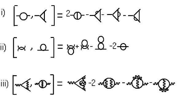
Figure 1: Assorted Lie brackets as examples: i) $\phi^{3}_{6}$ graphs, ii) $\phi^{4}_{4}$ graphs, iii) QED graphs.

Similarly, if form-factor decompositions are needed this can be incorporated using the notion of external structures or simply colorings of (sub-) graphs [5, 10].

1.2 The principle of multiplicative subtraction

Having defined Lie algebra structures on graphs, it is now easy to harvest them to derive the renormalization process. As announced, we just have to dualize the universal enveloping algebra ${\cal U(L)}$ of ${\cal L}$ and obtain a commutative, but not cocommutative Hopf algebra ${\cal H}$ [5]. To find this dual, one uses a Kronecker pairing and constructs it in accordance with the Milnor-Moore theorem [5, 7, 20].

We want to distinguish carefully now between the Hopf and Lie algebras of Feynman graphs, so we write $\delta_{\Gamma}$ for the multiplicative generators of the Hopf algebra and write $Z_{\Gamma}$ for the dual basis of the universal enveloping algebra of the Lie algebra ${\cal L}$ with pairing

$$\langle Z_{\Gamma},\delta_{\Gamma^{\prime}}\rangle=\delta^{K}_{\Gamma,\Gamma^{\prime}},$$ (5)

where on the rhs we have the Kronecker $\delta^{K}$, and extend the pairing by means of the coproduct

$$\langle Z_{\Gamma_{1}}Z_{\Gamma_{2}},X\rangle=\langle Z_{\Gamma_{1}}\otimes Z_{\Gamma_{2}},\Delta(X)\rangle.$$ (6)

First of all, we start by considering one-particle irreducible graphs as the linear generators of the Hopf algebra, with their disjoint union as product. We then identify the Hopf algebra as described above by a coproduct $\Delta:{\cal H}\to{\cal H}\otimes{\cal H}$:

$$\Delta(\Gamma)=\Gamma\otimes 1+1\otimes\Gamma+\sum_{\gamma{\subset}\Gamma}\gamma\otimes\Gamma/\gamma,$$ (7)

where the sum is over all unions of one-particle irreducible (1PI) superficially divergent proper subgraphs and we extend this definition to products of graphs so that we get a bialgebra. The above sum should, when needed, also run over appropriate projections to formfactors, to specify the appropriate type of local insertion [5] which appear in local counterterms, which we omitted in the above sum for simplicity. Fig.(2) gives examples of coproducts for various theories.

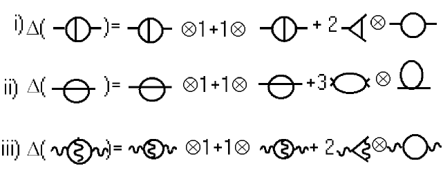
Figure 2: Assorted coproducts $\Delta(\Gamma)$: i) $\phi^{3}_{6}$, ii) $\phi^{4}_{4}$, iii) QED.

A short remark on notation: for any Hopf algebra element $X$ we often write a shorthand for its coproduct

$$\Delta(X)=\widetilde{\Delta}(X)+X\otimes 1+1\otimes X=X\otimes 1+1\otimes X+X^{\prime}\otimes X^{\prime\prime}.$$

Let now $X$ be a 1PI graph. For each term in the sum $\widetilde{\Delta}(X)=\sum_{i}X_{(i)}^{\prime}\otimes X_{(i)}^{\prime\prime}$ we have unique gluing data $G_{i}$ such that

$$X=X_{(i)}^{\prime\prime}\ast_{G_{i}}X_{(i)}^{\prime},\;\forall i.$$ (8)

These gluing date describe the necessary bijections to glue the components $X_{(i)}^{\prime}$ back into $X_{(i)}^{\prime\prime}$ so as to obtain $X$: given the right gluing data, we can reassemble the whole from its parts.

Having a coproduct, we still need a counit and antipode (coinverse): the counit $\bar{e}$ vanishes on any non-trivial Hopf algebra element, $\bar{e}(1)=1,\,\bar{e}(X)=0$. At this stage we have a commutative, but typically not cocommutative bialgebra [21]. It actually is a Hopf algebra as the antipode in such circumstances comes for free as

$$S(\Gamma)=-\Gamma-\sum_{\gamma{\subset}\Gamma}S(\gamma)\Gamma/\gamma.$$ (9)

The next thing we need are Feynman rules, maps $\phi:{\cal H}\to V$ from the Hopf algebra of graphs ${\cal H}$ into an appropriate space $V$.

Over the years, we have invented many calculational schemes in perturbative quantum field theory, and hence it is of no surprise that there are many choices for this space. In any case, we will have for disjoint 1PI graphs $\phi(\Gamma_{1}\Gamma_{2})\equiv\phi(\Gamma_{2}\Gamma_{1})=\phi(\Gamma_{1})\phi(\Gamma_{2})$, $\forall\phi:{\cal H}\to V$, where $V$ is an appropriate target space for the evaluation of the graphs. Then, with the Feynman rules providing a canonical character $\phi$, we will have to make one further choice: a renormalization scheme. This is is a map $R:V\to V$, and we demand that is does not modify the UV-singular structure, and furthermore should obey

$$R(xy)+R(x)R(y)=R(R(x)y)+R(xR(y)),$$ (10)

an equation which guarantees the multiplicativity of renormalization and is at the heart of the Birkhoff decomposition to be discussed below: it tells us that elements in $V$ split into two parallel subalgebras given by the image and kernel of $R$ [9]. Algebras for which such a map exists are known as Rota–Baxter algebras, a subject of increasing importance recently [22, 23].

Finally, the principle of multiplicative subtraction emerges: we define a further character $S_{R}^{\phi}$ which deforms $\phi\circ S$ slightly and delivers the counterterm for $\Gamma$ in the renormalization scheme $R$:

$$S_{R}^{\phi}(\Gamma)=-R[\phi(\Gamma)]-R\left[\sum_{\gamma{\subset}\Gamma}S_{R}^{\phi}(\gamma)\phi(\Gamma/\gamma)\right]$$ (11)

which should be compared with the undeformed

$$\phi\circ S=-\phi(\Gamma)-\sum_{\gamma{\subset}\Gamma}\phi\circ S(\gamma)\phi(\Gamma/\gamma).$$ (12)

Then, the classical results of renormalization theory follow immediately [8, 20, 24]. We obtain the renormalization of $\Gamma$ by the application of a renormalized character

$$\Gamma\to S_{R}^{\phi}\star\phi(\Gamma)$$

and Bogoliubov’s $\bar{R}$ operation as

$$\bar{R}(\Gamma)=\phi(\Gamma)+\sum_{\gamma{\subset}\Gamma}S_{R}^{\phi}(\gamma)\phi(\Gamma/\gamma),$$ (13)

so that we have

$$S_{R}^{\phi}\star\phi(\Gamma)=\bar{R}(\Gamma)+S_{R}^{\phi}(\Gamma).$$ (14)

Here, $S_{R}^{\phi}\star\phi$ is an element in the group of characters of the Hopf algebra, with the group law given by

$$\phi_{1}\star\phi_{2}=m_{V}\circ(\phi_{1}\otimes\phi_{2})\circ\Delta,$$

so that the coproduct, counit and coinverse (the antipode) give the product, unit and inverse of this group, as befits a Hopf algebra. This Lie group has the previous Lie algebra ${\cal L}$ of graph insertions as its Lie algebra [5].

In the above, we have given all formulas in their recursive form. Zimmermann’s original forest formula solving this recursion is obtained when we trace our considerations back to the fact that the coproduct of rooted trees can be written in non-recursive form, and similarly the antipode [24]. We also note that the principle of multiplicative subtraction can be formulated in much greater generality, as it is a basic combinatorial principle; see for example [25] for another appearance of this principle.

1.3 The Bidegree

A fundamental notion is the bidegree of a 1PI graph. Usually, induction in perturbative QFT, aiming to prove a desired result, is carried out using induction over the loop number, an obvious grading for 1PI graphs. On quite general grounds, for our Hopf algebras there exists another grading, which is actually much more useful. We call it the bidegree, ${\rm bid}(\Gamma)$ [10, 26]. To motivate it, consider a superficially divergent $n$-loop graph $\Gamma$ which has no divergent subgraph. It is evident that its short-distance singularities can be treated by a single subtraction, for any $n$. It is not the loop number, but the number of divergent subgraphs, which is the most crucial notion here. Fortunately, this notion has a precise meaning in the Hopf algebra of superficially divergent graphs using the projection into the augmentation ideal, a projection which has the scalars $q1\equiv qe$ as its kernel. This indeed counts the degree in renormalization parts of a graph: an overall superficially convergent graph has bidegree zero by definition, a primitive Hopf algebra element has bidegree one, and so on.

So we have ${\cal H}=\bigoplus_{i=0}^{\infty}{\cal H}^{(i)}$, with ${\rm bid}({\cal H}^{(i)})=i$. To define this decomposition, let ${\cal H}_{\rm Aug}$ be the augmentation ideal of the Hopf algebra, and let $P:{\cal H}\to{\cal H}_{\rm Aug}$ be the corresponding projection $P={\rm id}-E\circ\bar{e}$, with $E(q)=q1\in{\cal H}$. Let $\widetilde{\Delta}(X)=\Delta(X)-1\otimes X-X\otimes 1$, as before. $\widetilde{\Delta}$ is still coassociative, and for any $X\in{\cal H}_{\rm Aug}$ there exists a unique maximal $k$ such that $\widetilde{\Delta}^{k-1}(X)\in[{\cal H}^{(1)}]^{\otimes k}.$ Here, ${\cal H}^{(1)}$ is the linear span of primitive elements $y$: $\Delta(y)=y\otimes 1+1\otimes y$. We call this maximal $k$ the bidegree of a graph $\Gamma$.

As an example, the reader might determine the bidegree of the graphs in Figs.(1,2) and can check that it is homogeneous under the Lie bracket as well as under the coproduct and under the product (disjoint union). Typically, all properties connected to questions of renormalization theory can be proven more efficiently using the grading by the bidegree instead of the loop number, a point which deserves some detailed comment.

1.4 Renormalization and Hochschild Cohomology

Each Feynman graph $\Gamma$ can be written in the form $\Gamma=B_{+}^{\gamma,G_{X}}(X)$, where $\gamma$ is a bidegree one graph, $X$ is a collection of subdivergences of $\Gamma$ such that, when we shrink them all to a point in $\Gamma$, $\gamma$ remains, and $G_{X}$ is some data which tells us where to insert these subdivergences. Any such map $B_{+}^{\gamma,G_{X}}$ extends to a map on the Hopf algebra which is a closed Hochschild one-cocycle [10, 20].

This suggests a particularly nice way to prove locality of counterterms and finiteness of renormalized Green functions, by using the Hochschild closedness of the operator $B_{+}^{\gamma,G_{X}}$. Indeed it raises the bidegree by one unit and is therefore a natural candidate to obtain such bounty. Underlying this approach is the kinship between the Hopf algebras of Feynman graphs with the universal Hopf algebra of non-planar rooted trees, which has a very simple Hochschild cohomology [20, 27].

We will proceed by an induction over the bidegree, which is much more natural than the usual induction over the number of loops. So assume that $S_{R}\star\phi(\Gamma)$ is finite and $S_{R}(\Gamma)$ a local counterterm for all $\Gamma$ with ${\rm bid}(\Gamma)\leq k$. Show these properties for all $\Gamma$ with ${\rm bid}(\Gamma)=k+1$.

The start of the induction is easy: at unit bidegree, $\phi(\Gamma)-R[\phi(\Gamma)]$ is finite and $S_{R}(\Gamma)$ is local by assumption on $R$.

Let us assume we have established the desired properties of $S_{R}$ and $S_{R}\star\phi$ acting on all Hopf algebra elements up to bidegree $k$. Assume ${\rm bid}(\Gamma)=k+1$. We have

$$\Gamma=B_{+}^{\gamma,G}(X),$$ (15)

where ${\rm bid}(\gamma)=1$, ${\rm bid}(X)=k$, $X$ some monomial in the Hopf algebra.

Next,

$$\Delta(\Gamma)=B_{+}^{\gamma,G}(X)\otimes 1+\left[1\otimes B_{+}^{\gamma,G}\right]\Delta(X),$$ (16)

which expresses the crucial fact that $B_{+}^{\gamma,G}$ is a closed Hochschild one-cocycle.

Using the Hochschild closedness of $B_{+}^{\gamma,G}$ one immediately gets

$$S_{R}\star\phi(\Gamma)=S_{R}(\Gamma)+{\bf B}_{+}(\phi;S_{R}\star\phi;\gamma,G;X)$$ (17)

and

$$S_{R}(\Gamma)=-R[{\bf B}_{+}(\phi;S_{R}\star\phi;\gamma,G;X)].$$ (18)

Here we use a map ${\bf B}_{+}(\phi;S_{R}\star\phi;\gamma,G;X)$ which inserts the renormalized results $S_{R}\star\phi$ into the integral $\phi(\gamma)$ in accordance with the gluing data [9, 10].

From here, the induction step boils down to a simple estimate using the fact that the powercounting for asymptotically large internal loop momenta in $\phi(\gamma)$ is modified by the insertion of $S_{R}\star\phi(X)$ (which is finite by assumption, having bidegree $k$) only by powers of logarithms of internal momenta of $\gamma$, and that delivers the result easily, using the standard integral representation by the Feynman rules

$$\phi(\Gamma)=\int\prod_{e\in\Gamma^{[1]}_{\rm int}}d^{D}k_{e}\;P^{-1}(k_{e})\prod_{v\in\Gamma^{[0]}}\delta^{(D)}\left(\sum_{j\in f_{v}}k_{j}\right)g(v),$$ (19)

with a suitable ordering of propagators and vertices understood. A finite renormalization to achieve not only finiteness, but for example to resurrect the gauge invariance of the theory, can be incorporated in this approach via a further convolution with a character of the Hopf algebra. Details of such an approach will be the subject of future work.

This ends the review of the basic notions of renormalization theory. It remains to comment on progress which was initiated by this algebraic viewpoint along two lines: a connection to the Riemann–Hilbert problem [5, 6] and strong hints towards connections with number theory, coming from the values of residues of bidegree one graphs [11], as well as from the structure of the Dyson–Schwinger equations, but also arising from number theory itself [28]. But first, let us review the connection to the Riemann–Hilbert problem.

1.5 The Birkhoff decomposition and the renormalization group

Where do we stand now? We have recognized the iterative subtraction mechanism of perturbative quantum field theory as a Hopf algebra structure. The Bogoliubov recursion designed to guarantee local counterterms originates in very natural Lie and Hopf algebra structures of graphs, and thus forest formulas have been given their mathematical identification. The Lie group of characters on this Hopf algebra is based on a rather huge Lie algebra of antisymmetrized graph insertions. It has as many generators as there are 1PI graphs, and even if we restrict ourselves to the primitive (bidegree one) graphs into which any graph decomposes, we still are confronted with an infinite number of those, if our theory is renormalizable. Still, the algebraic structures reported so far allow for surprising new insight into the structure of QFT. A first such step is the recognition of the algebraic constraint on the renormalization map $R$. It leads to a Birkhoff decomposition which relates QFT to the Riemann–Hilbert problem [5, 6]. This certainly gives hope for a better understanding of the analytic structure of Green functions, as they now start looking like a generalization of other solutions to a Riemann–Hilbert problem, with KZ equations and hypergeometric functions coming to mind.

Further progress was made upon recognition of the role diffeomorphisms of physical parameters play in this context: group homomorphisms from the group of characters of Feynman graphs to diffeomorphisms of physical parameters are provided galore by QFT, and the Birkhoff decomposition is compatible with these homomorphisms: an unrenormalized physical observable has a decomposition into a bare and a renormalized part, a result which summarizes in one line the wisdom of locality and the renormalization group [6]. Still, the link towards the Riemann–Hilbert problem reveals the deficiencies of perturbative quantum field theory quite pointedly: the decomposition makes sense only in an infinitesimal disk, the order of the pole is unbounded and the diffeomorphism is anyhow only a formal one. The latter point cries for resummation, and the former points, as we will argue, demand some renormalization group improvement of perturbation theory, based on a factorization of graphs to be discussed below, to restore the credibility of perturbation theory as an input in any means to come to conclusions on the non-perturbative theory.

The Feynman rules in dimensional or analytic regularization determine a character $\phi$ on the Hopf algebra which evaluates as a Laurent series in a complex regularization parameter $\varepsilon$, with poles of finite order, this order being bounded by and hence dependent on the bidegree of the Hopf algebra element to which $\phi$ is applied. In minimal subtraction, $\phi_{-}:=S^{\phi}_{R=MS}$ has similar properties: it is a character on the Hopf algebra which evaluates as a Laurent series in a complex regularization parameter $\varepsilon$, with poles of finite order, this order being bounded by the bidegree of the Hopf algebra element to which $S^{\phi}_{R=MS}$ is applied, only that there will be no powers of $\varepsilon$ which are $\geq 0$. Then, $\phi_{+}:=S^{\phi}_{R=MS}\star\phi$ is a character which evaluates in a Taylor series in $\varepsilon$; all poles are eliminated. We have the Birkhoff decomposition

$$\phi=\phi_{-}^{-1}\star\phi_{+}.$$ (20)

This establishes an amazing connection between the Riemann–Hilbert problem and renormalization [5, 6]. It uses in a crucial manner once more that the multiplicativity constraints Eq.(10),

$$R[xy]+R[x]R[y]=R[R[x]y]+R[xR[y]],$$

ensure that the corresponding counterterm map $S_{R}$ is a character as well,

$$S_{R}[xy]=S_{R}[x]S_{R}[y],\;\forall x,y\in H,$$ (21)

by making the target space of the Feynman rules into a Rota–Baxter algebra, characterized by this multiplicativity constraint. The connection between Rota–Baxter algebras and the Riemann–Hilbert problem, which lurks in the background here, remains largely unexplored as of today.

As announced, renormalization in the MS scheme can now be summarized in a single phrase: with the character $\phi$ given by the Feynman rules in a suitable regularization scheme and well-defined on any small curve around $\varepsilon=0$, find the Birkhoff decomposition $\phi_{+}(\varepsilon)=\phi_{-}\star\phi$.

The unrenormalized analytic expression for a graph $\Gamma$ is then $\phi[\Gamma](\varepsilon)$, the MS-counterterm is $S_{{MS}}(\Gamma)\equiv\phi_{-}[\Gamma](\varepsilon)$ and the renormalized expression is the evaluation $\phi_{+}[\Gamma](0)$. Once more, note that the whole Hopf algebra structure of Feynman graphs is present in this group: the group law demands the application of the coproduct, $\phi_{+}=\phi_{-}\star\phi\equiv S_{MS}^{\phi}\star\phi$.

But still, one might wonder what a huge group this group of characters really is. What one confronts in QFT is the group of diffeomorphisms of physical parameters: lo and behold, changes of scales and renormalization schemes are just such (formal) diffeomorphisms. So, for the case of a massless theory with one coupling constant $g$, for example, this just boils down to formal diffeomorphisms of the form

$$g\to\psi(g)=g+c_{2}g^{2}+\ldots.$$

The group of one-dimensional diffeomorphisms of this form looks much more manageable than the group of characters of the Hopf algebras of Feynman graphs of such a theory.

1.6 Diffeomorphisms of physical parameters

Thus, it would be very nice if the whole Birkhoff decomposition could be obtained at the level of diffeomorphisms of the coupling constants. This is certainly most desirable from a physicists’ viewpoint: after all, we would like to have the theory parametrized by physical observables, and changes we can make in our way of formulating the theory should correspond to changes we can make in those observables.

The crucial step toward that goal is to realize the role of a standard QFT formula of the form (in the context of $\phi^{3}_{6}$ theory, say)

$$g_{\rm new}=g_{\rm old}\;Z_{1}Z_{2}^{-3/2},$$ (22)

which expresses how to obtain the new coupling in terms of a diffeomorphism of the old. This was achieved in [6], recognizing this formula as a Hopf algebra homomorphism from the Hopf algebra of diffeomorphisms to the Hopf algebra of Feynman graphs, regarding $Z_{g}=Z_{1}/\;Z_{2}^{3/2}$, a series over counterterms for all 1PI graphs with the external leg structure corresponding to the coupling $g$, in two different ways. It is at the same time a formal diffeomorphism in the coupling constant $g_{\rm old}$ and a formal series in Feynman graphs. As a consequence, there are two competing coproducts acting on $Z_{g}$. That both give the same result defines the required homomorphism, which transposes to a homomorphism from the largely unknown group of characters of ${\cal H}$ to the one-dimensional diffeomorphisms of this coupling.

The crucial fact in this is the recognition of the Hopf algebra structure of diffeomorphisms by Connes and Moscovici [29]: Assume you have formal diffeomorphisms $\phi,\psi$ in a single variable

$$x\to\phi(x)=x+\sum_{k>1}c_{k}^{\phi}x^{k},$$ (23)

and similarly for $\psi$. How do you compute the Taylor coefficients $c^{\phi\circ\psi}_{k}$ for the composition $\phi\circ\psi$ from the knowledge of the Taylor coefficients $c_{k}^{\phi},c_{k}^{\psi}$? It turns out that it is best to consider the Taylor coefficients

$$\delta_{k}^{\phi}=\log(\phi^{\prime}(x))^{(k)}(0)$$ (24)

instead, which are as good to recover $\phi$ as the usual Taylor coefficients. The answer lies then in a Hopf algebra structure:

$$\delta^{\phi\circ\psi}_{k}=m\circ(\tilde{\psi}\otimes\tilde{\phi})\circ\Delta_{CM}(\delta_{k}),$$ (25)

where $\tilde{\phi},\tilde{\psi}$ are characters on a certain Hopf algebra ${\cal H}_{CM}$ (with coproduct $\Delta_{CM}$) so that $\tilde{\phi}(\delta_{i})$ $=$ $\delta_{i}^{\phi}$, and similarly for $\tilde{\psi}$. Thus one finds a Hopf algebra with abstract generators $\delta_{n}$ such that it introduces a convolution product on characters evaluating to the Taylor coefficients $\delta_{n}^{\phi},\delta_{n}^{\psi}$, such that the natural group structure of these characters agrees with the diffeomorphism group. This is a very small piece of the work in [29], which was very crucial though in understanding the connection between the group of diffeomorphisms of physical parameters and the group of characters on our Hopf algebra ${\cal H}$: it turns out that this Hopf algebra of Connes and Moscovici is intimately related to rooted trees in its own right [20], signalled by the fact that it is linear in generators on the rhs, as are the coproducts of rooted trees and graphs [7, 20].

There are a couple of basic facts which enable one to make in general the transition from this rather foreign territory of the abstract group of characters of a Hopf algebra of Feynman graphs (which, by the way, equals the Lie group assigned to the Lie algebra with universal enveloping algebra the dual of this Hopf algebra) to the rather concrete group of diffeomorphisms of physical observables. These steps are:

• Recognize that $Z$ factors are given as counterterms over formal series of graphs starting with 1, graded by powers of the coupling, hence invertible.

• Recognize the series $Z_{g}$ as a formal diffeomorphism, with Hopf algebra coefficients.

• Establish that the two competing Hopf algebra structures of diffeomorphisms and graphs are consistent in the sense of a Hopf algebra homomorphism.

• Show that this homomorphism transposes to a Lie algebra and hence Lie group homomorphism.

This works out extremely well, with details given in [6]. In particular, the effective coupling $g_{\rm eff}(\varepsilon)$ now allows for a Birkhoff decomposition in the space of formal diffeomorphisms:

Theorem 2

[6]

$$g_{\rm eff}(\varepsilon)=g_{\rm eff-}(\varepsilon)^{-1}\circ g_{\rm eff+}(\varepsilon)$$ (26)

where $g_{\rm eff-}(\varepsilon)$ is the bare coupling and $g_{\rm eff+}(0)$ the renormalized effective coupling.

The above results hold as they stand for any massless theory which provides a single coupling constant, with the relevant Hopf algebra homomorphism for example in the QED case given by $e_{\rm new}=Z_{3}^{-1/2}e_{\rm old}$ (and $Z_{3}$ regarded as a sum over all 1PI vacuum polarization diagrams). If there are multiple interaction terms in the Lagrangian, one finds similar results relating the group of characters of the corresponding Hopf algebra to the group of formal diffeomorphisms in the multidimensional space of coupling constants.

Finally, the Birkhoff decomposition of a loop, $\delta(\varepsilon)\in{\rm Diff}\,(X),$ admits a beautiful geometric interpretation [6], described in Fig.(3).

Figure 3: A geometric picture for the Birkhoff decomposition [6]. Here, $\delta$ is the character obtained from $\phi$ by evaluating it as a complex number on an infinitesimal loop around the point of interest $\epsilon=0$, and $\delta_{\pm}$ are the components of its Birkhoff decomposition which induce transitions (formal diffeomorphisms) in the fiber $X$.

So what stops us from using this connection to the Riemann–Hilbert problem and establishing quantum field theory as a solution to this problem? There are two topics here: first of all, we are up to now talking about formal series, and a resummation is certainly needed to turn our formal diffeomorphisms into actual ones. Here, recent progress by Ramis [30] with formal series in connection with the Riemann–Hilbert problem, even in the case of zero radius of convergence, hopefully proves very relevant. It is in particular encouraging to see the emergence of ”ambiguity groups” [28, 30] appearing in this context: a proper identification of the renormalization group in terms of a Galois symmetry is one of the ideas which has slowly emerged in recent years.

But even before resummation, for each term in the perturbation series, the finite value is not necessarily the right input parameter for such a resummation. There are well-known deficiencies of perturbation theory [31, 32]:

• the subtraction of a counterterm in perturbation theory renders ambiguous dependencies on logarithms of scales in the renormalized amplitudes which are not to be trusted as such, and in conflict with the requirements from the renormalization group. A multiscale expansion seems to capture the essence of scaling in QFT more faithfully. Nevertheless, the exactness of perturbation theory is striking, and overcoming this obstacle without the sacrifice of the achievements of momentum space Feynman diagram perturbation theory would be most desirable.

• Iterating chains of one-loop graphs can produce renormalons in perturbation theory. On occasion, they can be used to parametrize the unknown regime of the non-perturbative, but are in the end just a suspicious infinite sum of the previous obstacle.

• $S_{R}^{\phi}(\Gamma)$, for ${\rm bid}(\Gamma)>1$, is a Laurent series which has poles of higher order, though all subdivergences have been eliminated in that local counterterm. It would be more natural, and desirable for our Riemann–Hilbert decomposition, if the pole term would be only of first order, say, after absorbing the subdivergences: a uniform bound, independent of the bidegree of $\Gamma$, on the order of the pole term would make our Riemann–Hilbert problem much more regular, even if the coefficients of that finite order pole still form a series in the coupling with vanishing radius of convergence. The appearance of higher order poles is again related to the first obstacle, as they arise from an iteration of scaling degrees coming from subdivergences calculated in perturbation theory. These poles are indeed completely determined by the residues in the theory [6], and can be obtained from the scattering-type formula of [6], with combinatorial coefficients which turn out to be generalized factorials [9, 33], by that formula. These poles are thus highly redundant and again reflect our inefficient handling of scaling properties in perturbation theory.

• at higher loop orders, poles appear which are arbitrarily close to the region of interest (a little disk around $\epsilon=0$), which typically come from the expansion of $\Gamma(1\pm n\epsilon)$ in perturbation theory, with $n$ being the loop number. Again, the appearance of these poles at $\pm\;1/n$ can be traced back to the same origin as the previous obstacles. These poles force us (for large loop number) to consider an infinitesimal disk around $\epsilon=0$ in the Birkhoff decomposition.

Alas, the logarithmic scaling properties of perturbation theory are not in accordance with the exact renormalization group and to overcome this difficulty, and to understand better the relation between perturbative and non-perturbative approaches, again the Lie algebra of Feynman graphs offers assistance. This is a very new development, and we will in the next section just outline some recent work in progress, partially mentioned already in [10]. We start by motivating factorizations in quantum field theory.

2 Perspective: Euler products in QFT

In this section we want to comment on a connection between Dyson–Schwinger equations and Euler products. Ultimately, I believe that there is a deep connection between the two subjects, and to motivate this connection let us start with a subject from number theory, the Riemann $\zeta$ function, and obtain it as a solution to a Dyson–Schwinger equation. For now, this is only meant as a sufficient stimulus to invert the reasoning and look for Euler products in quantum field theory.

2.1 The Riemann $\zeta$ function from a Dyson–Schwinger equation

The Riemann $\zeta$-function is the analytic continuation of the sum $\sum_{n}1/n^{s}$, and can be written in the form of an Euler product

$$\zeta(s)=\sum_{n}\frac{1}{n^{s}}=\prod_{p}\frac{1}{1-p^{-s}},\;\Re(s)>1,$$ (27)

where the product is over all primes $p$ of the (rational) integers.

Let us now define a Hopf algebra of sequences $(p_{1},\ldots,p_{k})$, where the $p_{i}$ are primes, and introduce $B_{+}^{p}[J]$ as the sequence which is obtained by adding a new prime $p$ as the first element to the sequence $J$, for example $B_{+}^{3}[(5,3,2)]=(3,5,3,2)$. The Hopf algebra structure emerges when we require that $B_{+}^{p}$ is Hochschild closed for all $p$:

$$\Delta(B_{+}^{p}[J])=B_{+}^{p}[J]\otimes 1+[{\rm id}\otimes B_{+}^{p}]\Delta[J],$$ (28)

with $\Delta(1)=1\otimes 1$ and where we identify $1$ with the empty sequence. Define the value $w(J)$ to be the product of the entries of $J$, and let the symmetry factor $S(J)$ be $k!$ if the sequence has length $l(J)=k$, which avoids overcounting below. Note that for a one element sequence $(p)$,

$$\Delta[(p)]=(p)\otimes 1+1\otimes(p),$$ (29)

primitive elements have prime value, $w((p))=p$.

Consider the ”Dyson–Schwinger equation”

$$\overline{\zeta}(\rho)=1+\rho\sum_{p}B_{+}^{p}[\overline{\zeta}(\rho)],$$ (30)

so that we obtain a formal series (in ”the coupling” $\rho$)

$$\overline{\zeta}(\rho)=1+\rho\sum_{p}(p)+\rho^{2}\sum_{p_{1},p_{2}}(p_{1},p_{2})+\cdots.$$ (31)

Define ”Feynman rules” by $\phi_{s}(J)=\frac{1}{l(J)!}w(J)^{-s}$, and set

$$\zeta(s,\rho)=\phi_{s}[\overline{\zeta}(\rho)].$$ (32)

Then, we recover Riemann’s $\zeta$ function as

$$\zeta(s)=\lim_{\rho\to 1}\zeta(s,\rho).$$ (33)

Note the general structure of the formal “Dyson–Schwinger equation” above: it determines an unknown $\zeta(\rho)$ in terms of itself, as ”1 plus a sum over the image of the unknown $\zeta(\rho)$ under all closed Hochschild one cocycles $B_{+}^{p}$, weighted by appropriate symmetry factors”.

Next, we remind ourselves that $\zeta(s)$ has an Euler product. Is there an Euler product for $\overline{\zeta}$?

The answer is yes, and the simplest way is to get it from the well-known shuffle product on sequences. We introduce this associative and commutative product via

$$B_{+}^{p_{1}}(J_{1})\sqcup B_{+}^{p_{2}}(J_{2})=B_{+}^{p_{1}}(J_{1}\sqcup B_{+}^{p_{2}}(J_{2}))+B_{+}^{p_{2}}(B_{+}^{p_{1}}(J_{1})\sqcup J_{2}).$$ (34)

Then,

$$\overline{\zeta}(\rho)=\Pi_{p}^{\sqcup}\frac{1}{1-\rho\;(p)},\;{\mbox{where}}\;\frac{1}{1-\rho\;(p)}=1+\rho\;(p)+\rho^{2}\;(p)\sqcup(p)+\cdots,$$ (35)

and where the shuffle product is used in the Euler product throughout. We then have

$$\zeta(s)={\phi_{s}}_{\mid_{\rho=1}}\left(\Pi_{p}^{\sqcup}\frac{1}{1-\rho\;(p)}\right)=\Pi_{p}\frac{1}{1-p^{-s}},$$ (36)

the evaluation of the product is the product of the evaluations.

The reason we dared calling the above equation a Dyson–Schwinger equation is a simple fact - the true Dyson–Schwinger equations of QFT have a similar structure: they express an unknown Green function as a sum over all possible insertions of itself in all possible skeleton diagrams. This allows us to write the unknown Green function as a sum over all possible images over all closed Hochschild one-cocycles in the theory (the $B_{+}^{\gamma}$ obtained by summing over all possible gluing data $G_{i}$ in the $B_{+}^{\gamma,G_{i}}$ considered earlier), precisely provided by the primitive (bidegree one) graphs $\gamma$, which play the role of primes. Let us review quickly their fascinating properties first.

2.2 Residues in QFT

Consider a Feynman graph in some renormalizable quantum field theory and assume the graph is free of superficially divergent subgraphs. We can always restrict ourselves to logarithmically divergent graphs by factorizing out suitable polynomials in masses and external momenta. Then, such a logarithmic divergent quantity has a residue which is independent of all these parameters. It is a well-defined number and the only chance we have of changing this number is to change the topology of the graph under consideration. So that should be a rather interesting number, and indeed, nature rewards us for posing a good question by revealing an intimate connection between the topology of the graph and the number-theoretic residues one obtains upon evaluating such a graph. The residue here is the coefficient of the short-distance singularity in such a graph, calculated as the coefficient of the first order pole in dimensional regularization, or even as a residue in the operator-theoretic sense. As our graph has bidegree one, it provides a residue which is a universal number independent of the choice of a regularization. Topologically, the simplest graphs are ladder graphs. Their residues are rational numbers [11].

Then, the next class of graphs are graphs which have a less trivial topology, reflected by a non-trivial Gauss code, $(1,2,1,2)$ being the first such topology given in Fig.(4), see [11]. By all computational experience, graphs which have such a Gauss code deliver a residue $\sim\zeta(3)$. From there, a whole universe unfolds, revealing deep connections between the symmetries in a QFT, and its transcendental richness [11].

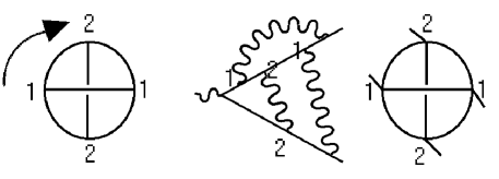
Figure 4: Non-exhaustive list of examples of QFT graphs realizing the Gauss code diagram $\{1,2,1,2\}$ (on the left), related to the appearance of $\zeta(3)$ in their evaluation. The two Feynman graphs are from $\phi^{4}_{4}$ and QED. Only internal vertices matter.

One remarkable fact is that the decomposition into two-line reducible parts corresponds to a factorization of graphs which is compatible with their evaluation: the evaluation of the full graph delivers the product of the evaluation of the parts, as in the product of prime knots [11, 12, 13].

There is no space here to comment on the weird and wonderful data with which renormalizable QFT provide us in such circumstances, with fascinating new phenomena appearing at higher loop orders [34], and we refer the reader to [11] for an exhaustive census of such phenomena. But still, one fact is worth mentioning: the relation between the presence or absence of transcendental numbers depending on the internal symmetries in the theory, a connection which started with Rosner’s observation [35] of the absence of $\zeta(3)$ in the residues of QED at three loops, and which has found even more striking confirmation ever since, but still deserves much further exploration [11, 36].

Also, there are two basic structures in Feynman graphs: the convolution of renormalization schemes

$$S_{R_{1}}^{\phi}\star\phi=[S_{R_{1}}^{\phi}\star S_{R_{2}}^{\phi}\circ S]\star[S_{R_{2}}^{\phi}\star\phi],$$ (37)

which generalizes Chen’s lemma [9], and the generalized shuffle identity

$$\phi(\Gamma_{1}\vee\Gamma_{2})\sim\phi(\Gamma_{1})\phi(\Gamma_{2}),$$ (38)

the factorization to be introduced below. In structure, they are very similar to the relations which appear amongst generalized polylogarithms [18] and Euler–Zagier sums, the number class most obviously related to Feynman diagrams, even if they might not yet exhaust them. For now, radiative correction calculations have stimulated many a development in that area of number theory. Number theory in return hopefully is able to further our understanding of QFT, in particular with respect to an identification of a QFT by its transcendental nature, eventually.

2.3 Factorizing graphs

Let us now ask the question wether a factorization into Euler products can be found in quantum field theory? And then, if this can be found on the combinatorial level, will the evaluation, by the Feynman rules, equal the product of the evaluations, and, if not, by how much will it deviate?

After all, a typical Dyson–Schwinger equation is of the form

$$X=1+\sum_{\gamma}B_{+}^{\gamma}(g^{k}[\cup_{k}X]),$$ (39)

where the infinite sum in the Hopf algebra is over primitive graphs $\gamma$, $k=k(\gamma)$ is the degree of $\gamma$, and as the notation indicates, the maps $B_{+}^{\gamma}$ are closed Hochschild one-cocycles, and the sum is over all of those. $X$ is here to be regarded as an infinite sum of graphs contributing to a chosen Green function, and evaluation by the Feynman rules delivers the usual Dyson–Schwinger equations given as an integral equation over the kernels provided by the primitive graphs $\gamma$. Note that, as insertion into a primitive graph commutes with the coproduct in the desired way, we can directly read off the renormalized Dyson–Schwinger equation as

$$X_{R}=Z_{X}+\sum_{\gamma}B_{+}^{\gamma}(g^{k}[\cup_{k}X_{R}]),$$ (40)

where $Z_{X}$ is the negative part in the Birkhoff decomposition with respect to a renormalization scheme $R$. Here, $[\cup_{k}X]$ indicates a $k$-fold disjoint union of $X$, regarded as the product in the Hopf algebra of graphs.

Actually, we typically have a coupled set of such equations with several unknowns (Green functions) but we here simply discuss the structure of such equations, suitable generalizations being straightforward.

So the natural question to ask is: is there an Euler product for the formal sum generated by such an equation? The answer is indeed affirmative.

The crucial step lies in the definition of the product $\vee$ which generalizes the shuffle product $\sqcup$, appropriate for totally ordered sequences, to the partial order given by being a subgraph.

Let us briefly describe this product: let a sequence of primitive graphs $J=(\gamma_{1},\ldots,\gamma_{k})$ be given. We say that a graph $\Gamma$ is compatible with that sequence, $\Gamma\sim J$, iff its bidegree equals the length $k$ of the sequence and

$$\langle Z_{\gamma_{k}}\otimes\ldots\otimes Z_{\gamma_{1}},\tilde{\Delta}^{k-1}(\Gamma)\rangle\not=0,$$

where we use the previous pairing between the Lie algebra elements $Z_{\gamma}$ and the Hopf algebra. Let $n_{\Gamma}$ be the number of sequences compatible with $\Gamma$. Define

$$\Gamma_{1}\vee\Gamma_{2}=\sum_{{I_{1}\sim\Gamma_{1}\atop I_{2}\sim\Gamma_{2}}}\sum_{\Gamma\sim I_{1}\sqcup I_{2}}\frac{1}{n_{\Gamma}}\Gamma,$$ (41)

where the first sum is over all sequences compatible with the two graphs $\Gamma_{1},\Gamma_{2}$ and the second sum is over all sequences appearing in the shuffle of $I_{1},I_{2}$, and over all compatible graphs $\Gamma$. This is a commutative associative product on 1PI graphs. It has a relation to the pre-Lie product introduced earlier, to be described elsewhere. Then, we have

Theorem 3

$X=\prod^{\vee}_{\gamma}\frac{1}{1-g^{k(\gamma)}\gamma},$

the proof of which is elementary given the definition of the product $\vee$, which maps 1PI graphs to 1PI graphs.

Most urgently needed is an understanding to what extent this is compatible with the evaluation by Feynman rules $\phi$: how much can we say about

$$\phi\left(\Pi^{\vee}_{\gamma}\frac{1}{1-\gamma}\right)\;\mbox{vs}\;\Pi_{\gamma}\frac{1}{1-\phi(\gamma)}=\zeta_{G}(\phi)\;?$$

Here, $\zeta_{G}(\phi)$ shall be regarded as a “$\zeta$ function” (in quotes, as we do not give here any non-trivial results concerning functional relations or such) which, for a fixed Green function $G$ has an Euler product over the primitive (bidegree one) graphs $\gamma$ (which all have a graphical residue ${\rm\bf res}(\gamma)$ which agrees with the tree level contribution to $G$) and where the variable $\phi$ is the chosen character on the Hopf algebra of graphs underlying the QFT in which the Green function appears.

To phrase it otherwise, what stops us from actually considering an Euler product over all primitive graphs to get a formal solution to the Dyson–Schwinger equations in general? Can we just construct $\zeta$-functions associated to a chosen Green function, defined via an Euler product over primitive elements?

A few comments are immediate: no, perturbation theory does not factorize straightforwardly into its primitives. But there are many encouraging signs. First of all, the scattering type formulas of [6] show that in dimensional regularization the leading coefficient of the singularity respects the desired factorization. This is useful. Indeed, for arbitrary superficially divergent graphs $\Gamma_{1},\Gamma_{2}$ one immediately shows

$$\frac{\phi(\Gamma_{1}\ast_{v}\Gamma_{2}))}{\phi(\Gamma_{1})\phi(\Gamma_{2})}=\frac{n_{1}+n_{2}}{n_{2}}(1+{\cal O}(\epsilon)),$$ (42)

where $n_{1},n_{2}$ are the numbers of loops in $\Gamma_{1},\Gamma_{2}$ and $\epsilon$ is the dimensional regularization parameter (similarly in other regularizations).

The combinatorial pre-factor $(n_{1}+n_{2})/n_{2}$ is easy to understand and to deal with. It is in the non-leading terms where progress had to be made. But let us muse a bit about what the consequences of such a factorization would be. Using the definition of $S_{R}^{\phi}$, one immediately has, for products of primitives,

$$\phi(\gamma_{1}\ast_{v}\gamma_{2})=\phi(\gamma_{1})\phi(\gamma_{2}) \Leftrightarrow S_{R}^{\phi}(\gamma_{1}\ast_{v}\gamma_{2})$$

$$=-R\left[\phi(\gamma_{1})\phi(\gamma_{2})-R[\phi(\gamma_{2})]\phi(\gamma_{1})\right] = -R[\phi(\gamma_{1})(\phi(\gamma_{2})-R[\phi(\gamma_{2})])],$$ (43)

which evidently has only a first order pole, and that property remains true for arbitrary products of primitives, and hence for the whole Hopf algebra, if and only if $\phi$ is multiplicative. Actually, most of the deficiencies of perturbation theory vanish if we can evaluate with a $\phi$ which is a character with respect to the product $\ast$, or $\vee$, for that matter.

The two crucial steps towards such a factorization, which amounts to a partial resummation of graphs, are
- a requirement to absorb vertex subdivergences in Green functions which depend only on a single scale, so that the beneficial properties of one-parameter groups of scaling come to bear, a requirement which sits very comfortably with the fact that gauge theories relate vertex subdivergences to self-energies [37],
- an appropriate use of the renormalization group in the Dyson–Schwinger equations, which allows us to describe the presence or absence of factorization in a controlled way in relation to the fixpoint behaviour of the $\beta$-function of the theory.

That the renormalization group enters is quite obvious: the structure of the Euler product as a product over geometric series over residues of primitive graphs excludes any proliferation as associated with a renormalon, a fact which by itself suggests that if we are to achieve such a factorization, the renormalization group should play a role. So these type of questions are certainly of interest, and results along these lines will be pointed out in upcoming work.

Finally, let us mention a first simple example as to how basic algebraic structures of our graph insertions relate to physical properties of a theory.

Proposition 4

i) The product $\Gamma_{1}\vee\Gamma_{2}$ is integral for 1PI graphs in $\phi^{3}_{6}$ and $\phi^{4}_{4}$.
ii) It is non integral for QED: $\Gamma_{1}\vee\Gamma_{2}=0\Rightarrow$ $\Gamma_{1}=0$ or $\Gamma_{2}=0$ or $\Gamma_{1}=\Gamma_{2}=\;\raisebox{-2.84526pt}{\epsfbox{vvp.eps}}\;$.

But now, the Hopf algebra of QED graphs can be divided by an appropriate ideal of graphs $\Gamma$ containing    (the ideal of graphs $\Gamma$ such that  $\Delta^{bid(\Gamma)-1}(\Gamma)$ has    as an element) and in the quotient -in which our product is integral- it turns out that the Ward identities hold automatically. The proposition has a generalization to non-abelian gauge theories which is under scrutiny at the moment.

The final aspect in our outlook on QFT is about symmetries in the Dyson–Schwinger equations which can relate them to differential Galois groups. The equations are integral equations of a complicated kind. But they still offer a lot of the symmetries also known from differential equations. So a few short comments along the lines of [10] shall finish this section.

2.4 Galois Groups and Feynman Graphs

There are many symmetries in a Dyson–Schwinger equation, which reveal themselves as invariants under the permutation of places where to insert subgraphs, so they are reflected by identities between pole terms of graphs. We have an obvious ring structure we are dealing with, using products $\Gamma_{1}\vee\Gamma_{2}$ of 1PI graphs. We start drifting towards a treatment of Feynman graphs as a ring, with associated field of fractions say, where the role of primes is played by primitive graphs, and an Euler product combined with an appropriate shuffle identity for Feynman rules should guide us towards an appropriate notion of a $\zeta$-function for a given Green function. To get an idea what these symmetries are related to, we remind ourselves that in the skeleton expansion of a Dyson–Schwinger equation we sum over all possible insertion places (gluing data). Indeed, the resulting series over graphs can be written using elementary symmetric polynomials in the insertion places, $\gamma^{[0]}$ say, of the skeleton $\gamma$.

So consider the combination $\Gamma_{1}(\ast_{i}-\ast_{j})\Gamma_{2}$, the difference of the insertion of a subgraph $\Gamma_{2}$ into $\Gamma_{1}$ at two different places $i,j$.

Following [7, 10] we can consider the ”differential equation” (here, $Z_{[{\bf res}(\Gamma_{2}),\Gamma_{2}]}$ $(X)$ is a derivation which replaces $\Gamma_{2}$ by its tree-level counterpart ${\bf res}(\Gamma_{2})$ in $X$)

$$Z_{[{\bf res}(\Gamma_{2}),\Gamma_{2}]}(X)=\Gamma_{1},$$ (44)

which is solved by the bidegree two Hopf algebra element $X=\Gamma_{1}\ast_{i}\Gamma_{2}$ as well as by the bidegree two $X=\Gamma_{1}\ast_{j}\Gamma_{2}$. Furthermore, the bidegree one primitive $X=\Gamma_{1}(\ast_{i}-\ast_{j})\Gamma_{2}$ solves the homogeneous equation

$$Z_{[{\bf res}(\Gamma_{2}),\Gamma_{2}]}(X)=0,$$ (45)

where we assume throughout that $\Gamma_{1}$ and $\Gamma_{2}$ are of bidegree one. If one linearizes a Dyson–Schwinger equation and restricts it to a finite number of underlying skeletons, the equation, rewritten as a differential equation, has many structural similarities with differential equations which have regular singularities, as also the above argument exemplifies. This suggests to connect the insertion of subgraphs at various different places with Galois symmetries, and is the motivation to indeed look at invariants under such symmetries in Feynman graphs, with a beautiful first result reported in [38]: the coefficient of the highest weight transcendental in the residues of two graphs connected by such a symmetry is invariant. While this is obvious, thanks to the scattering type formula, for the coefficient of the highest pole in the regularization parameter, it is indeed a very subtle result for the residue in a graph of large bidegree.

2.5 Summary

The interplay between number theory, noncommutative geometry and perturbative quantum field theory reveals, to my mind, strong hints towards the structure of quantum field theory. Many of the ideas featured here are not to be brought to fruition quickly, but to my mind it is a fascinating task for a theorist to unravel the structures of the theories which have been most successful so far in our description of nature, and which have been carefully extracted from experimental evidence by the high energy and condensed matter theoretical physics communities. The combinatorial structures of renormalization with the relation to the Riemann–Hilbert problem, the appearance of Euler–Zagier sums as residues of diagrams, and the factorization properties of the Dyson–Schwinger equations all point towards fundamental mathematical structures. Recent ideas and progress in pure mathematics [28, 30] point towards quantum field theory. We finally might get the message.

CNRS-IHES, 35 Route de Chartres, F91440 Bures-sur-Yvette, France;
Center for Math.-Phys., Boston Univ., Boston MA02215, USA.

References

- [1] J. Zinn-Justin, Quantum Field Theory and Critical Phenomena, Oxford Univ. Press (2002, 4th Ed.).
- [2] D. Espriu, J. Manzano and P. Talavera, Flavor mixing, gauge invariance and wave-function renormalisation, Phys. Rev. D 66, 076002 (2002) [arXiv:hep-ph/0204085].
- [3] M. Marino, Chern-Simons theory, matrix integrals, and perturbative three-manifold invariants, [arXiv:hep-th/0207096].
- [4] G. ’t Hooft, M. Veltman, DIAGRAMMAR, Cern report 73/9 (1973), reprinted in ”Particle interactions at very high energies”. NATO Adv. Study Inst. Series, Sect. B, vol. 4B, 177.
- [5] A. Connes, D. Kreimer, Renormalization in quantum field theory and the Riemann-Hilbert problem. I: The Hopf algebra structure of graphs and the main theorem, Commun. Math. Phys. 210 249 (2000) [hep-th/9912092].
- [6] A. Connes, D. Kreimer, Renormalization in quantum field theory and the Riemann-Hilbert problem. II: The beta-function, diffeomorphisms and the renormalization group, Commun. Math. Phys. 216 215 (2001)[hep-th/0003188].
- [7] A. Connes and D. Kreimer, Insertion and elimination: The doubly infinite Lie algebra of Feynman graphs, Annales Henri Poincare 3, 411 (2002) [arXiv:hep-th/0201157].
- [8] D. Kreimer, On the Hopf algebra structure of perturbative quantum field theories, Adv. Theor. Math. Phys. 2 303 (1998)[q-alg/9707029].
- [9] D. Kreimer, Chen’s iterated integral represents the operator product expansion, Adv. Theor. Math. Phys. 3 627 (2000) [hep-th/9901099].
- [10] D. Kreimer, Structures in Feynman graphs - Hopf algebras and Symmetries, talk given at the Dennisfest, Stony Brook June 14-21, 2001 [hep-th/0202110], to appear.
- [11] D. Kreimer, Knots and Feynman Diagrams, Cambridge Univ. Press 2000.
- [12] D. J. Broadhurst, D. Kreimer, Knots and numbers in Phi**4 theory to 7 loops and beyond, Int. J. Mod. Phys. C6 519 (1995)[hep-ph/9504352].
- [13] D. J. Broadhurst, D. Kreimer, Association of multiple zeta values with positive knots via Feynman diagrams up to 9 loops, Phys. Lett. B393 403 (1997) [hep-th/9609128].
- [14] D. J. Broadhurst, J. A. Gracey and D. Kreimer, Beyond the triangle and uniqueness relations: Non-zeta counterterms at large N from positive knots, Z. Phys. C 75 559 (1997) [arXiv:hep-th/9607174].
- [15] D. J. Broadhurst, D. Kreimer, Renormalization automated by Hopf algebra, J. Symb. Comput. 27 581 (1999) [hep-th/9810087].
- [16] D. J. Broadhurst, D. Kreimer, Combinatoric explosion of renormalization tamed by Hopf algebra: 30-loop Pade-Borel resummation, Phys. Lett. B475 63 (2000) [hep-th/9912093].
- [17] D. J. Broadhurst, D. Kreimer, Exact solutions of Dyson-Schwinger equations for iterated one-loop integrals and propagator-coupling duality, Nucl. Phys. B 600 403 (2001) [hep-th/0012146].
- [18] A.B. Goncharov, Galois symmetries of fundamental groupoids and noncommutative geometry, math-ag/0208144.
- [19] D. Kreimer, Combinatorics of (perturbative) quantum field theory, Phys. Reports 363 387 (2002) [hep-th/0010059].
- [20] A. Connes, D. Kreimer, Hopf algebras, renormalization and noncommutative geometry, Commun. Math. Phys. 199 203 (1998) [hep-th/9808042].
- [21] C. Kassel, Quantum Groups, Springer 1995.
- [22] J.-L. Loday, M.O. Ronco, Trialgebras and families of polytopes, math-at/0205043, and references there.
- [23] K. Ebrahimi-Fard, Loday-type algebras and the Rota-Baxter relation, Lett. Math. Phys. 61 139 (2002) [math-ph/0207043].
- [24] D. Kreimer, On overlapping divergences, Commun. Math. Phys. 204 669 (1999) [hep-th/9810022].
- [25] F. Markopoulou, An algebraic approach to coarse graining, hep-th/0006199.
- [26] D. J. Broadhurst, D. Kreimer, Towards cohomology of renormalization: Bigrading the combinatorial Hopf algebra of rooted trees, Commun. Math. Phys. 215 217 (2000) [hep-th/0001202].
- [27] L. Foissy, Les algèbres des Hopf des arbres enracinés décorées, Thesis, Univ. Reims, Dept. of Math., available from the author: loic.foissy@univ-reims.fr (2001).
- [28] A. Connes, Symétries Galoisiennes et Renormalisation, Sém. Poincaré 2 75 (2002) [math.qa/0211199].
- [29] A. Connes, H. Moscovici, Hopf algebras, cyclic cohomology and the transverse index theorem, Commun. Math. Phys. 198 199 (1998) [math. dg/9806109].
- [30] J.-P. Ramis, Très anciennes et très nouvelles méthodes de sommation de séries divergentes, talk given at Colloque: Renormalization - Theory and Perspectives, IHES, Oct.14-18 2002.
- [31] V. Rivasseau, An Introduction to Renormalization, Sém. Poincaré 2 1 (2001).
- [32] A.S. Wightman, Some Lessons of Renormalization Theory, in ”The Lessons of Quantum Theory”, J. de Boer et.al. Eds., Elsevier 1986.
- [33] D. Kreimer, R. Delbourgo, Using the Hopf algebra structure of QFT in calculations, Phys. Rev. D60 105025 (1999) [hep-th/9903249].
- [34] P. Belkale, P. Brosnan, Matroids, motives and a conjecture of Kontsevich, math.ag/0012198.
- [35] J.L. Rosner, Phys. Rev. Lett. 17 1190 (1966); Ann. Phys. 44 11 (1967).
- [36] D.J. Broadhurst, R. Delbourgo, D. Kreimer, Unknotting the polarized vacuum of quenched QED, Phys. Lett. B366 421 (1996) [hep-ph/9509296].
- [37] A.A. Slavnov, Regularization-Independent Gauge-Invariant Renormalization of the Yang–Mills Theory, Theor. Math. Phys. 130(1) 1 (2002).
- [38] I. Bierenbaum, R. Kreckel, D. Kreimer, On the invariance of residues of Feynman graphs,, J. Math. Phys. 43 4721 (2002) [hep-th/0111192].