CU-TP-1072

hep-th/0211124

Brane gas cosmology in M-theory:
late time behavior

Richard Easther^a, Brian R. Greene^ab, Mark G. Jackson^c

and Daniel Kabat^c

^aInstitute for Strings, Cosmology and Astroparticle Physics

Columbia University, New York NY 10027

^bDepartment of Mathematics

Columbia University, New York, NY 10027

^cDepartment of Physics

Columbia University, New York, NY 10027

We investigate the late-time behavior of a universe containing a supergravity gas and wrapped 2-branes in the context of M-theory compactified on $T^{10}$. The supergravity gas tends to drive uniform expansion, while the branes impede the expansion of the directions about which they are wrapped. Assuming spatial homogeneity, we study the dynamics both numerically and analytically. At late times the radii obey power laws which are determined by the brane wrapping numbers, leading to interesting hierarchies of scale between the wrapped and unwrapped dimensions. The biggest hierarchy that could evolve from an initial thermal fluctuation produces three large unwrapped dimensions. We also study configurations corresponding to string winding, in which the M2-branes are all wrapped around the (small) 11th dimension, and show that this recovers the scenario discussed by Brandenberger and Vafa.

1 Introduction

The dual realizations that D-branes are an intrinsic component of string theory [1] and that the five distinct vacua of string theory are actually different limits of eleven-dimensional M-theory [2] have had dramatic implications for cosmology. Both developments widen the range of options open to model-builders, but they also increase the number of constraints that a successful “string” cosmological model must satisfy. In particular, branes have given rise to a huge number of new models, which typically postulate that our apparently three dimensional universe is actually a 3-brane embedded in a higher dimensional background [3]. Even in “standard” cosmological models, however, branes are expected to be in thermal equilibrium with other matter in the early universe, and must therefore be incorporated into any complete cosmological scenario.

Brane gas cosmology is devoted to understanding the cosmological role of the “gas” of branes that inhabited the early universe. A particular focus of this program has been whether brane gas cosmologies single out a special number of “large” dimensions. In 1989, Brandenberger and Vafa argued that cosmological models containing a gas of winding strings can produce, at most, three macroscopic dimensions [4]. This work has been tested and extended in a number of ways since then [5, 6, 7, 8, 9, 10, 11, 12]. The key observation underlying this work is that extended, $p$ dimensional objects have $p+1$ dimensional worldvolumes, and from a purely topological perspective these worldvolumes will only intersect in $2(p+1)$ spacetime dimensions or less. Thus, strings can only interact in three spatial dimensions (or less), whereas 2-branes can find each other in up to five spatial dimensions. One obviously hopes that Brandenberger and Vafa’s conclusion that strings naturally lead to a three dimensional universe is not undermined when branes are added to the picture. Indeed Alexander, Brandenberger and Easson [8] have argued that when branes are included, strings will still dominate the evolution of the universe at late times, so the basic Brandenberger-Vafa mechanism survives.

This paper extends brane gas cosmology in two important ways. First, rather than work with ten dimensional string theory, we take eleven-dimensional M-theory as our starting point. This is a natural basis for any theory that hopes to understand the origin of the three large dimensions, since string theory is itself a compactification of M-theory, with the compact direction providing the string dilaton [2]. Consequently, string theory implicitly assumes that one direction is already on a different footing from the rest, and in the long run we would hope to explain this rather than inject it as a hypothesis. Second, rather than using solely thermodynamic arguments, we study the dynamical evolution of an M-theoretic universe containing M2-branes and a gas of supergravity particles. We ignore the M5-branes that are present in the M-theory spectrum, since they can annihilate in the full 11 dimensional M-theory spacetime. We are particularly interested in cases where the different directions (assumed to be toroidally compactified) are anisotropically wrapped by M2-branes. We develop the equations of motion for the general case in which each of the 10 spatial dimensions is distinguishable from the others, and describe the configuration of wrapped branes and anti-branes with a “wrapping matrix”. Although we assume a toroidal topology, numerical and analytical results [11] indicate that wrapping dynamics should be insensitive to topology, and hence we believe our conclusions extend to more realistic compactifications.

Strings are obtained when one dimension of the M2-branes gets wrapped on the 11th dimension, which is taken to be much smaller than the Planck scale. Similarly, D-branes in string theories can be obtained as various configurations of M2- and M5-branes. Thus we no longer need to consider five separate brane gas cosmology scenarios, one for each string theory: our goal is to see if we can use M-theoretic models to make generic predictions about the overall form of the universe.

Motivated by the original Brandenberger-Vafa scenario, we focus on the late time asymptotics of universes with a subspace that has no wrapping modes, presenting both an analytic discussion and specific numerical solutions. Here we are primarily concerned with what is possible, rather than what is probable, and focus on the most interesting initial states that are permitted by general topological arguments. In a subsequent paper we will discuss the thermodynamics of a brane dominated universe in more detail, in order to establish the relative likelihood of different initial states. Consequently, we pay most attention to the following scenario. We imagine that thermal fluctuations drive subspaces of various dimensions to momentarily expand to a larger than average size. If the fluctuation involves a five dimensional subspace, interesting nontrivial dynamics can ensue. Fully wrapped 2-brane/anti-2-brane pairs will generically annihilate in five space dimensions, thereby removing their restoring force. This leaves partially wrapped 2-branes that have one dimension wrapped along the expanding five-space and one dimension wrapped along one of the other, smaller dimensions. From an effective five-dimensional perspective, such branes appear to be wrapped one-dimensional objects – strings – and naively appear to impede further expansion. Yet, we imagine that subsequent thermal fluctuations within this five-dimensional environment will, once again, drive various subspaces to expand further, and if such a subspace should happen to have three (or fewer) dimensions, the effective wrapped strings will be able to annihilate, thus allowing the subspace to expand without further constraint. We therefore see the possibility of generating an interesting hierarchy with a large three dimensional subspace emerging from an intermediate five dimensional subspace, with all remaining dimensions small [8]. One of our goals is to study this scenario in detail to determine if the dynamics leverages the topological reasoning we have used and drives a hierarchy between the dimensions.

In Section 2 we derive the equations of motion and discuss some of their general properties. In section 3 we present numerical solutions to the equations of motion, and in section 4 we study the behavior at late times analytically. In section 5 we consider string winding, to make contact with the original scenario of Brandenberger and Vafa. In section 6 we discuss the implications of our results, and outline possibilities for future work.

2 Homogeneous brane gas dynamics

Our models are governed by M-theory which is well-described by eleven-dimensional supergravity when the radii and curvature scales are larger than the eleven-dimensional Planck length. This assumption will be justified in hindsight, as the cosmologically relevant solutions we obtain contain growing radii. We consider two types of matter. The first is the massless supergravity spectrum consisting of 128 bosonic and 128 fermionic degrees of freedom – we ignore massive modes since we expect that these will quickly decay. The second ingredient is wrapped M2-branes. Although M-theory also contains M5-branes, these will annihilate quickly in 10+1 dimensions and thus should not be significant to the late-time behavior. We assume that the M2-branes are at rest and ignore fluctuations on the brane volume, as these effects are subleading in our large radii assumption. Finally, to make the analysis tractable, we assume that the particle and brane gases are homogeneous.

Using the metric ansatz

$$ds^{2}=-dt^{2}+\sum_{i=1}^{d}\bigl{(}R_{i}(t)\bigr{)}^{2}d\theta_{i}^{2}\qquad 0\leq\theta_{i}\leq 2\pi$$ (1)

the non-vanishing Christoffel symbols are

$$\Gamma^{t}_{ij}=\delta_{ij}R_{i}\dot{R}_{i},\qquad\Gamma^{i}_{tj}=\Gamma^{i}_{jt}=\delta^{i}{}_{j}{\dot{R}_{i}\over R_{i}},$$ (2)

while the non-vanishing components of the Einstein tensor are

$$G^{t}{}_{t} = {1\over 2}\sum_{k\not=l}{\dot{R}_{k}\dot{R}_{l}\over R_{k}R_{l}},$$ (3)

$$G^{i}{}_{i} = \sum_{k\not=i}{\ddot{R}_{k}\over R_{k}}+{1\over 2}\sum_{k\not=l}{\dot{R}_{k}\dot{R}_{l}\over R_{k}R_{l}}-\sum_{k\not=i}{\dot{R}_{k}\dot{R}_{i}\over R_{k}R_{i}},$$ (4)

where there is no implied summation on $i$ in the second line.

We first introduce a gas of massless supergravity particles, with energy density $\rho_{\rm S}$ and pressure $p_{\rm S}$. For simplicity we take the gas to be homogeneous and isotropic, with a perfect fluid stress tensor

$$T^{\mu}{}_{\nu}={\rm diag}(-\rho_{\rm S},p_{\rm S},\ldots,p_{\rm S})\,.$$ (5)

The equation of state appropriate for $d$ spatial dimensions fixes $p_{\rm S}={1\over d}\rho_{\rm S}$, while covariant conservation of the stress tensor requires

$$\rho_{\rm S}={{\rm const.}\over V^{(d+1)/d}}\,,$$ (6)

where the volume of the $d$ dimensional torus is simply

$$V=\prod_{i}{2\pi R_{i}}\,.$$ (7)

The second source of stress-energy in our model universe is a gas of 2-branes, wrapped on the various cycles of the torus. These are characterized by a matrix of wrapping numbers $N_{ij}$, where we take $N_{i<j}$ to represent the number of branes wrapped on the $(ij)$ cycle, while $N_{i>j}$ represents the number of antibranes. A single M2-brane is described by the Nambu-Goto action

$$S = -T_{2}\int d^{3}\xi\sqrt{-\det g_{\alpha\beta}}$$ (8)

$$g_{\alpha\beta} = \partial_{\alpha}X^{\mu}\partial_{\beta}X^{\nu}g_{\mu\nu}$$ (9)

where the brane tension $T_{2}={1\over(2\pi)^{2}\ell_{11}^{3}}$. This leads to the stress tensor

$$T^{\mu\nu}=-T_{2}\int d^{3}\xi\delta^{11}(X-X(\xi))\sqrt{-\det g}\,g^{\alpha\beta}\partial_{\alpha}X^{\mu}\partial_{\beta}X^{\nu}\,.$$ (10)

For simplicity we assume that the branes are at rest, and ignore any possible excitations on the brane worldvolumes. Then, for a single brane wrapped on the $(12)$ cycle and uniformly smeared over the transverse $T^{d-2}$, the stress tensor is

$$T^{\mu}{}_{\nu}=-{T_{2}\over 2\pi R_{3}\cdots 2\pi R_{d}}{\rm diag}(1,1,1,0,\ldots,0)\,.$$ (11)

With a matrix of wrapping numbers, the non-zero components of the brane gas stress tensor are

$$T^{t}{}_{t} = -{T_{2}\over V}(2\pi)^{2}\sum_{k\not=l}R_{k}R_{l}N_{kl}$$ (12)

$$T^{i}{}_{i} = -{T_{2}\over V}(2\pi)^{2}\sum_{k\not=i}R_{k}R_{i}\left(N_{ki}+N_{ik}\right)$$ (13)

with no sum on $i$ in the second line.

We now insert these two sources of energy-momentum into the right hand side of the $d$-dimensional Einstein equations,

$$G^{\mu}{}_{\nu}=-8\pi GT^{\mu}{}_{\nu}$$ (14)

where the gravitational coupling is

$$16\pi G=(2\pi)^{8}\ell_{11}^{9}\,.$$ (15)

The time-time equation can be solved for the energy density and hence pressure of the supergravity gas,

$$8\pi G\rho_{\rm S}={1\over 2}\sum_{k\not=l}{\dot{R}_{k}\dot{R}_{l}\over R_{k}R_{l}}-{8\pi GT_{2}\over V}(2\pi)^{2}\sum_{k\not=l}R_{k}R_{l}N_{kl}\,.$$ (16)

After a little re-arrangement, the space-space equations yield the following set of second-order differential equations for the radii.

$${\ddot{R}_{i}\over R_{i}} = {8\pi GT_{2}\over V}\left[{2d+1\over d(d-1)}\,(2\pi)^{2}\sum_{k\not=l}R_{k}R_{l}N_{kl}-(2\pi)^{2}\sum_{k\not=i}R_{k}R_{i}\left(N_{ki}+N_{ik}\right)\right]$$ (17)

$$+{1\over 2d}\sum_{k\not=l}{\dot{R}_{k}\dot{R}_{l}\over R_{k}R_{l}}-\sum_{k\not=i}{\dot{R}_{k}\dot{R}_{i}\over R_{k}R_{i}}\,.$$

2.1 Some exact solutions

With no wrapped branes ($N_{ij}=0$) the model reduces to an 11 dimensional radiation dominated universe, and it is easy to find a number of exact solutions. In particular, with the ansatz

$$R_{i}(t)=c_{i}\left(t-t_{0}\right)^{\alpha_{i}}$$ (18)

we find the following solutions to (17):

• Flat spacetime, with $\alpha_{1}=\cdots=\alpha_{d}=0$, in which case $\rho_{\rm S}$ will vanish.

• Kasner solutions, with $\sum_{i}\alpha_{i}=\sum_{i}(\alpha_{i})^{2}=1$. The energy density $\rho_{\rm S}$ vanishes, so these are vacuum solutions. Note that the exponents $\alpha_{i}$ must lie in the interval $[-1,1]$, and that at least one of the $\alpha_{i}$’s must be negative.

• Radiation dominated, with $\alpha_{1}=\cdots=\alpha_{d}={2\over d+1}$. The energy density of the radiation is non-zero, fixed by the constraint (16).

One can also find a solution with brane wrapping but no gravitons, in which we set $N_{ij}=n$ for all $i\not=j$ but take $\rho_{\rm S}=0$. Using the same ansatz (18), but setting all the $R_{i}$ equal (so that $c_{i}=c$ and $\alpha_{i}=\alpha$), demanding that $\rho_{\rm S}=0$ implies

$${\alpha^{2}\over 2(t-t_{0})^{2}}={8\pi GT_{2}n\over(2\pi R)^{d-2}}\,.$$ (19)

This equation is solved for all times by setting $\alpha={2\over d-2}$, and choosing the value of $c$ appropriately. Given these values, one can check that the $\ddot{R}_{i}$ equations (17) are also satisfied.

The ansatz (18) doesn’t give the most general solution to the equations of motion, since we ought to be able to specify $2d$ independent initial radii and velocities.

2.2 General features

To study the solutions of the field equations (17), it is convenient to work in terms of new variables $\lambda_{i}(t)\equiv\log{(2\pi R_{i}(t))}$ introduced in [5]. The field equations become

$$\ddot{\lambda_{i}}+{\dot{\rm V}\over{\rm V}}\dot{\lambda}_{i}=8\pi G\left({1\over d}\rho_{\rm S}+{3\over d-1}\rho_{\rm B}\right)-{8\pi GT_{2}\over V}e^{\lambda_{i}}\sum_{j\not=i}(N_{ij}+N_{ji})e^{\lambda_{j}}\,.$$ (20)

The volume of the spatial torus is

$$V=e^{\sum_{i}\lambda_{i}}\,,$$ (21)

the energy density from brane tension is

$$\rho_{\rm B}={T_{2}\over V}\sum_{i\not=j}e^{\lambda_{i}}e^{\lambda_{j}}N_{ij}$$ (22)

and the energy density from supergravity excitations is fixed by the constraint (16)

$$8\pi G\rho_{\rm S}={1\over 2}\sum_{i\not=j}\dot{\lambda_{i}}\dot{\lambda_{j}}-8\pi G\rho_{\rm B}.$$ (23)

As noted in [5], this system of equations can be regarded as describing a non-relativistic particle moving in $d$ dimensions. The particle has a coefficient of friction, given by $\dot{V}/V$, due to the expansion of the universe. A position-dependent force acts on the particle, given by the right hand side of (20). This force consists of two terms. The first term,

$$F_{i}^{(1)}=8\pi G\left({1\over d}\rho_{\rm S}+{3\over d-1}\rho_{\rm B}\right)\,,$$ (24)

is positive definite and is the same for every value of $i$. It drives a uniform expansion of the universe. The second term,

$$F_{i}^{(2)}=-{8\pi GT_{2}\over V}e^{\lambda_{i}}\sum_{j\not=i}(N_{ij}+N_{ji})e^{\lambda_{j}}\,,$$ (25)

is either zero or negative and it suppresses the growth of dimensions with large wrapping numbers. In the M-theory context, this is the mechanism by which anisotropic wrapping numbers lead to an anisotropic expansion of the universe. Another way of stating this is to note that the equations of motion (20) imply that

$$\ddot{\lambda}_{i}-\ddot{\lambda}_{j}+{\dot{V}\over V}(\dot{\lambda}_{i}-\dot{\lambda}_{j})=8\pi G(p_{i}-p_{j})$$ (26)

where $p_{i}$ is the pressure exerted on the $i{}^{\hbox{\em th}}$ dimension. Thus differential pressures, of the sort exerted by an anisotropic brane gas, lead to differential expansion rates.

Let us comment on some general properties of these equations. First note that the volume of the torus increases monotonically with time. This follows from rewriting the constraint (23) in the form

$$\left({\dot{V}\over V}\right)^{2}=\left(\sum_{i}\dot{\lambda}_{i}\right)^{2}=\sum_{i}(\dot{\lambda}_{i})^{2}+16\pi G\left(\rho_{\rm S}+\rho_{\rm B}\right)\,.$$ (27)

The right hand side is positive definite for all nontrivial models, vanishing only for the trivial case of periodically identified Minkowski space. We can choose the direction of time to make $\dot{V}>0$.

The rest of this paper is primarily concerned with models where the wrapping matrix $N_{ij}$ is anisotropic. Motivated by our discussion in section 1, we assume that the spatial dimensions fall into three classes. We refer to a direction $i$ such that $N_{ij}=N_{ji}=0$ for all $j$ as unwrapped. Directions $i$ for which $N_{ij}$ and $N_{ji}$ are nonzero except for those $j$ corresponding to an unwrapped direction are referred to as fully wrapped. Directions $i$ where some of the $N_{ij}$ or $N_{ji}$ are zero for values of $j$ which are not unwrapped are referred to as partially wrapped. That is, listing dimensions in the order unwrapped, partially wrapped, fully wrapped, the wrapping matricies we will consider look like

$$\left(\begin{array}[]{cccccccccc}\cdot&0&0&0&0&0&0&0&0&0\\ 0&\cdot&&0&0&0&0&0&0&0\\ 0&0&\cdot&0&0&0&0&0&0&0\\ 0&0&0&\cdot&0&N_{4,6}&N_{4,7}&N_{4,8}&N_{4,8}&N_{4,10}\\ 0&0&0&0&\cdot&N_{5,6}&N_{5,7}&N_{5,8}&N_{5,9}&N_{5,10}\\ 0&0&0&N_{6,4}&N_{6,5}&\cdot&N_{6,7}&N_{6,8}&N_{6,9}&N_{6,10}\\ 0&0&0&N_{7,4}&N_{7,5}&N_{7,6}&\cdot&N_{7,8}&N_{7,9}&N_{7,10}\\ 0&0&0&N_{8,4}&N_{8,5}&N_{8,6}&N_{8,7}&\cdot&N_{8,9}&N_{8,10}\\ 0&0&0&N_{9,4}&N_{9,5}&N_{9,6}&N_{9,7}&N_{9,8}&\cdot&N_{9,10}\\ 0&0&0&N_{10,4}&N_{10,5}&N_{10,6}&N_{10,7}&N_{10,8}&N_{10,9}&\cdot\end{array}\right)$$ (28)

The diagonal entries in the matrix are irrelevant. In this example the directions 1 through 3 are unwrapped, 4 and 5 partially wrapped, and 6 through 10 fully wrapped (assuming all the $N_{ij}$ written out explicitly in the above matrix are non-zero).

Now consider what happens when $m$ dimensions are unwrapped and $d-m$ dimensions are either partially or fully wrapped. We introduce

$$\mu = \sum_{i=1}^{m}\lambda_{i}=\log\,\,(\hbox{\rm volume of unwrapped torus}),$$ (29)

$$\Lambda = \sum_{i=m+1}^{d}\lambda_{i}=\log\,\,(\hbox{\rm volume of wrapped torus})\,.$$ (30)

Summing over the appropriate values of $i$, and using the definition of $\rho_{\rm B}$, we find the following differential equations for $\mu$ and $\Lambda$:

$$\ddot{\mu}+(\dot{\mu}+\dot{\Lambda})\dot{\mu} = 8\pi G\left({m\over d}\rho_{\rm S}+{3m\over d-1}\rho_{\rm B}\right)$$ (31)

$$\ddot{\Lambda}+(\dot{\mu}+\dot{\Lambda})\dot{\Lambda} = 8\pi G\left({d-m\over d}\rho_{\rm S}+{d-3m+2\over d-1}\rho_{\rm B}\right)$$ (32)

The overall character of the dynamics depends on $m$. For small $m$, both terms in the right hand side for $\ddot{\Lambda}$ are positive, and if $\dot{\Lambda}$ is zero, then the second derivative must be positive, leading to a local minimum. Conversely, with a larger value of $m$, the right hand side of this equation has both a positive and a negative term, and both local maxima and minima are allowed. For $\mu$ there can never be a negative term on the right hand side, so if these directions are initially expanding they will then expand forever.

When $d-3m+2$ vanishes the brane tension does not contribute to the growth of the internal dimensions. This picks out a special dimensionality of the unwrapped subspace, for which the internal dimensions have nearly constant radii. When $d=10$ this occurs for $m=4$.

Perhaps the most important feature of these equations, which we analyze in more detail in section 4, is that an attractor mechanism governs the behavior at late times. That is, the radii at late times are determined solely by the wrapping matrix, and are (up to some scaling symmetries discussed in section 4) independent of the initial radii and velocities. This is intuitively clear from examining the second term in the “force”, (25). Suppose one of the radii, say $R_{1}$, starts out with an unusually small (or large) value. This does not affect the force on $R_{1}$ itself, since $R_{1}$ appears in both the numerator and denominator of $F_{1}^{(2)}$. But the force on the other radii will become larger (or smaller), in such a way as to restore a balance between the different radii. This suggests that the behavior at late times is solely determined by the wrapping matrix.

3 Numerical results

We now present numerical solutions to the equations of motion (17). The technique is to start with a set of initial radii and velocities, then evolve the system both forwards and backwards in time using a Runge-Kutta routine. Motivated by our discussion in section 1, we assume a wrapping matrix with $m_{1}$ unwrapped dimensions, $m_{2}$ partially wrapped directions, and $m_{3}=d-m_{1}-m_{2}$ fully wrapped dimensions. For the specific case $m_{1}=3$ and $m_{2}=2$ in a ten dimensional universe we have the wrapping matrix given by (28). The wrapping numbers should be chosen based on an understanding of thermal fluctuations in the early universe. Pending this, for our numerical calculations we simply take the non-zero wrapping numbers to be randomly chosen integers $N_{ij}\in\{1,2,3\}$. We take the initial radii $R_{i}$ to be randomly chosen between 1 and 5 Planck lengths, and we take the initial velocities $\dot{R}_{i}$ to be randomly chosen between -0.5 and +0.5. A typical numerical solution for 3 unwrapped dimensions, 2 partially wrapped dimensions and 5 fully wrapped dimensions, is shown in Fig. 1. A solution for $m_{1}=3$, $m_{2}=4$ and $m_{3}=3$ is shown in Fig. 2.

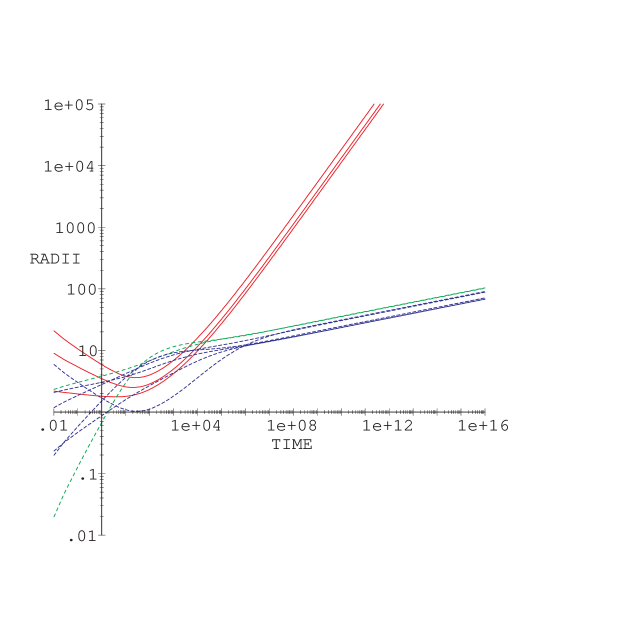
Figure 1: Radii vs. time for three unwrapped dimensions (solid red curves), two partially wrapped dimensions (dotted green curves) and five fully wrapped dimensions (dashed blue curves). Distances and and times measured in Planck units.

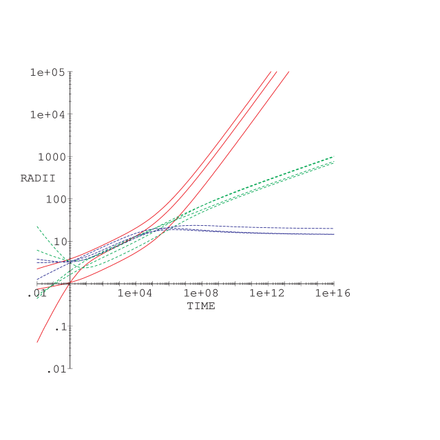
Figure 2: A plot with three unwrapped dimensions (solid red curves), four partially wrapped dimensions (dotted green curves) and three fully wrapped dimensions (dashed blue curves).

The equations predict that the early universe is radiation-dominated, with the volume of the spatial torus being ${\rm V}\sim t^{2d/(d+1)}$. Thus the universe originates in a big bang, which we have taken to be at $t=0$. The big bang is apparently highly anisotropic, with some radii increasing while others go to zero, but we do not trust our equations of motion at early times: the temperature diverges while many of the radii are sub-Planckian, so we do not expect supergravity to be valid. It would be interesting to understand what, if anything, resolves the initial singularity in M-theory. Presumably U-duality plays a role, perhaps along the lines that have been argued in string theory [4].

We do expect supergravity to hold at late times, due to the growing radii and falling temperature. The growing radii allow us to neglect brane–antibrane annihilation, which turns off as the universe expands, and excitations on the branes will get red-shifted away faster than the brane tension. We therefore trust our solutions to provide an accurate description of the system at late times, presumably until low-energy dynamics eventually stabilize the moduli.

Thus the most significant feature of these solutions is that, after a rather long transition period, the unwrapped radii begin to grow as a universal power of $t$. The partially and fully wrapped radii also grow as universal powers of $t$, but with different (smaller) exponents. This leads to the dynamical formation of a hierarchy between the wrapped and unwrapped directions. We will determine the power laws analytically in the next section.

To conclude, let us comment on a less generic feature of these solutions. As we will see in the next section, the exponents appearing in the late-time power laws depend only on the values of $m_{1}$, $m_{2}$, $m_{3}$. However the coefficients in front of the power laws depend have complicated dependence on the wrapping numbers. A wrapping matrix of the form (28) tends to make the partially wrapped dimensions bigger than the fully wrapped dimensions at late times. This effect can be seen in the figures, and suggests that brane gas cosmology also leads to a sub-hierarchy in the sizes of the internal dimensions. In the case of most interest, this suggests that one may end up with five small dimensions, two intermediate-sized dimensions, and three decompactified dimensions. Such a hierarchy has also been argued to emerge from weakly-coupled string theory [8].

The intriguing possibility of the dynamical hierarchy comes with a number of qualifications, however. We need a better understanding of thermal fluctuations at early times, to determine what sort of wrapping numbers are reasonable. In addition, in this scenario some low-energy mechanism must eventually stabilize the moduli, and it is quite possible that this mechanism will erase any hierarchy that forms.

4 Late time behavior

To complement our numerical results, we proceed to study the behavior of the radii at late times analytically. Rather remarkably, there is an attractor mechanism at work, giving late-time behavior that is independent of the initial radii and velocities.

We study the late-time behavior with $m_{1}$ unwrapped dimensions, $m_{2}$ partially wrapped dimensions and $m_{3}$ fully wrapped dimensions. That is, we consider wrapping matrices of the form of (28).

The late-time behavior of solutions to the equations of motion (17) is captured by the ansatz

$$2\pi R_{i}=e^{\lambda_{i}}=\left\{\begin{array}[]{ll}a_{i}t^{\alpha}&i=1,\ldots,m_{1}\quad\hbox{\rm(unwrapped)}\\ b_{i}t^{\beta}&i=m_{1}+1,\ldots,m_{1}+m_{2}\quad\hbox{\rm(partially wrapped)}\\ c_{i}t^{\gamma}&i=m_{1}+m_{2}+1,\ldots,d\quad\hbox{\rm(fully wrapped)}\,.\end{array}\right.$$ (33)

With this ansatz, the energy densities due to supergravity particles and brane tension are given by

$$\rho_{\rm S}=\left({{\rm const.}\over V}\right)^{(d+1)/d}=\left({{\rm const.}\over\prod a_{i}\prod b_{i}\prod c_{i}t^{m_{1}\alpha+m_{2}\beta+m_{3}\gamma}}\right)^{(d+1)/d}$$ (34)

$$\rho_{\rm B}={T_{2}\over\prod a_{i}\prod b_{i}\prod c_{i}t^{m_{1}\alpha+m_{2}\beta+m_{3}\gamma}}\times$$

$$\mbox{}\qquad\left(\sum_{i\not=j}(N_{ij}+N_{ji})b_{i}c_{j}t^{\beta+\gamma}+\sum_{i\not=j}N_{ij}c_{i}c_{j}t^{2\gamma}\right)\,.$$ (35)

There are several distinct classes of behavior at late times since, depending on the values of $m_{1}$, $m_{2}$, $m_{3}$, certain contributions to the energy density become negligible at late times. The following four subsections exhaust the possibilities.

4.1 Neglect $\rho_{\rm S}$

If the universe expands rapidly enough then it is brane-dominated at late times, with $\rho_{\rm B}\gg\rho_{\rm S}$. We begin by analyzing this case, which turns out to be the one of greatest physical interest.

Let us assume that every term in $\rho_{\rm B}$ makes a comparable contribution to the energy density. This amounts to assuming that $\beta=\gamma$. Substituting the ansatz (33) into the equations of motion (20), and neglecting $\rho_{\rm S}$, the time dependence cancels out of the equations of motion as long as

$$m_{1}\alpha+(m_{2}+m_{3}-2)\beta=2\,.$$ (36)

The equation of motion for each unwrapped dimension becomes

$$\alpha(m_{1}\alpha+(m_{2}+m_{3})\beta-1)={3\over d-1}8\pi Gt^{2}\rho_{\rm B}\,.$$ (37)

On the other hand, summing the equations of motion over all partially and fully wrapped dimensions (that is, from $i=m_{1}+1$ to $d$) gives

$$\beta(m2+m3)(m_{1}\alpha+(m_{2}+m_{3})\beta-1)=\left({3(m_{2}+m_{3})\over d-1}-2\right)8\pi Gt^{2}\rho_{\rm B}\,.$$ (38)

Comparing (37) and (38), one must have

$${\alpha\over(m_{2}+m_{3})\beta}={3\over d-3m_{1}+2}\,.$$ (39)

The solution to (36) and (39) is

$$\alpha = {6(d-m_{1})\over d(d-m_{1})+4m_{1}-4}$$ (40)

$$\beta=\gamma = {2d-6m_{1}+4\over d(d-m_{1})+4m_{1}-4}\,.$$

Note that the exponents depend on the spatial dimension $d$ and the number of unwrapped dimensions $m_{1}$, but not on $m_{2}$ or $m_{3}$ separately.

The late-time power law exponents are therefore fixed by $d$ and $m_{1}$. We now show that the coefficients in front of the power laws are also depend on the wrapping matrix. The ansatz (33) reduces the equations of motion to a set of algebraic equations. The equations of motion for the unwrapped dimensions are all identical, and give a single nontrivial equation. The equations of motion for the partially and fully wrapped dimensions give another $m_{2}+m_{3}$ equations. In addition equation (36) must be imposed. Thus we have a total of $m_{2}+m_{3}+2$ equations. Now let’s count the unknowns. Since $a_{i}$ appears only in the combination $\prod_{i}a_{i}$, there are a total of $m_{2}+m_{3}+3$ unknowns $\alpha$, $\beta=\gamma$, $\prod a_{i}$, $b_{i}$, $c_{i}$. Thus for generic wrapping numbers the equations are sufficient to determine all of the unknowns in terms of the wrapping matrix, up to a freedom to make rescalings

$$a_{i}\rightarrow\Omega a_{i}\qquad b_{i}\rightarrow\Omega^{-m_{1}/(m_{2}+m_{3}-2)}b_{i}\qquad c_{i}\rightarrow\Omega^{-m_{1}/(m_{2}+m_{3}-2)}c_{i}$$ (41)

which leave the equations invariant (for example, note that $\rho_{\rm B}$ is invariant under this rescaling).

This shows that there is an attractor mechanism at work. Modulo the scale symmetry (41), the late time behavior is determined solely by the wrapping matrix. That is, the system forgets about the initial values of the radii $R_{i}$ and velocities $\dot{R}_{i}$.

Of course, this analysis assumes that we can ignore $\rho_{\rm S}$. This is only consistent if

$$(m_{1}\alpha+m_{2}\beta+m_{3}\gamma)(d+1)/d>2$$ (42)

or equivalently

$$m_{1}<3d(d+2)/(7d+2)\,.$$ (43)

This analysis also assumes that all terms in $\rho_{\rm B}$ are comparable. By comparing to section 4.2, this requires $m_{3}>m_{2}$.

4.2 Neglect $\rho_{\rm S}$ and full-full wrapping

For a highly anisotropic wrapping, the partially and fully wrapped dimensions will behave differently at late times. To analyze this possibility, assume that $\gamma<\beta$. This makes the full–full wrapping terms in the brane energy density negligible at late times. Let’s also assume that $\rho_{\rm S}$ is negligible.

We get one equation by requiring that $\rho_{\rm B}\sim 1/t^{2}$, namely

$$m_{1}\alpha+(m_{2}-1)\beta+(m_{3}-1)\gamma=2\,.$$ (44)

The equation of motion for the unwrapped dimensions reads

$$\alpha(m_{1}\alpha+m_{2}\beta+m_{3}\gamma-1)={3\over d-1}8\pi Gt^{2}\rho_{\rm B}$$ (45)

while the sum of the equations of motion for the partially wrapped dimensions gives

$$m_{2}\beta(m_{1}\alpha+m_{2}\beta+m_{3}\gamma-1)=\left({3m_{2}\over d-1}-1\right)8\pi Gt^{2}\rho_{\rm B}$$ (46)

and for the fully wrapped

$$m_{3}\gamma(m_{1}\alpha+m_{2}\beta+m_{3}\gamma-1)=\left({3m_{3}\over d-1}-1\right)8\pi Gt^{2}\rho_{\rm B}\,.$$ (47)

This is sufficient to fix the exponents

$$\alpha = {6m_{2}m_{3}\over(d-4)m_{2}m_{3}+(d-1)(m_{2}+m_{3})}$$

$$\beta = {2m_{3}(3m_{2}-d+1)\over(d-4)m_{2}m_{3}+(d-1)(m_{2}+m_{3})}$$

$$\gamma = {2m_{2}(3m_{3}-d+1)\over(d-4)m_{2}m_{3}+(d-1)(m_{2}+m_{3})}$$

A little equation counting shows that the coefficients of the power laws are determined by the wrapping matrix, up to the freedom to make rescalings by

$$a_{i}\rightarrow\Omega a_{i}\qquad b_{i}\rightarrow\Omega^{-m_{1}/(m_{2}+m_{3}-2)}b_{i}\qquad c_{i}\rightarrow\Omega^{-m_{1}/(m_{2}+m_{3}-2)}c_{i}$$ (48)

and by

$$a_{i}\rightarrow a_{i}\qquad b_{i}\rightarrow\Omega^{1/(m_{2}-1)}b_{i}\qquad c_{i}\rightarrow\Omega^{-1/(m_{3}-1)}c_{i}\,.$$ (49)

This analysis assumes that $\gamma<\beta$, or equivalently that $m_{2}>m_{3}$. It also assumes that $\rho_{\rm S}$ is negligible, which is consistent if

$$(m_{1}\alpha+m_{2}\beta+m_{3}\gamma)(d+1)/d>2$$ (50)

or equivalently

$${m_{2}m_{3}\over m_{2}+m_{3}}>{d(d-1)\over 7d+2}\,.$$ (51)

4.3 Neglect full-full wrapping

Next assume that $\rho_{\rm S}$ makes an important contribution at late times, but that $\gamma<\beta$ so that the full–full wrapping terms in the brane energy density are negligible.

Requiring that $\rho_{\rm S}$ and $\rho_{\rm B}$ scale like $1/t^{2}$ gives two conditions on the exponents. Together with the equations of motion, this is sufficient to fix

$$\alpha = {2\over d+1}{d(m_{2}+m_{3})+2m_{2}m_{3}\over d(m_{2}+m_{3})-4m_{2}m_{3}}$$

$$\beta = {2\over d+1}{d(m_{2}-2m_{3})+2m_{2}m_{3}\over d(m_{2}+m_{3})-4m_{2}m_{3}}$$

$$\gamma = {2\over d+1}{d(m_{3}-2m_{2})+2m_{2}m_{3}\over d(m_{2}+m_{3})-4m_{2}m_{3}}$$

The coefficients in front of the power laws are fixed up to the rescaling freedom

$$a_{i}\rightarrow\Omega^{m_{2}-m_{3}}a_{i}\qquad b_{i}\rightarrow\Omega^{-m_{1}}b_{i}\qquad c_{i}\rightarrow\Omega^{m_{1}}c_{i}$$ (52)

which leaves $\rho_{\rm S}$ and the relevant terms in $\rho_{\rm B}$ invariant.

Neglecting the full–full wrapping is consistent if $\gamma<\beta$, or equivalently if $m_{2}>m_{3}$. By comparison with section 4.2, we need $m_{2}m_{3}/(m_{2}+m_{3})<d(d-1)/(7d+2)$ in order for $\rho_{\rm S}$ to make an important contribution.

4.4 All terms important

Finally, consider the possibility that all terms in the energy density are important. Plugging the ansatz (33) into the equations of motion the time dependence cancels provided that both $\rho_{\rm S}$ and $\rho_{\rm B}$ scale like $1/t^{2}$. If we assume that all contributions to $\rho_{\rm B}$ are equally important this fixes the exponents

$$\alpha = {3d-m_{1}\over m_{1}(d+1)}$$ (53)

$$\beta=\gamma = -{1\over d+1}\,.$$

Note that, just as in section 4.1, the exponents depend on $d$ and $m_{1}$, but not on $m_{2}$ or $m_{3}$ separately.

The equations of motion become a system of $m_{2}+m_{3}+1$ algebraic equations for the $m_{2}+m_{3}+1$ unknowns $\prod a_{i}$, $b_{i}$, $c_{i}$. In this case there is a true attractor mechanism at work: the unknowns are uniquely determined since the scale symmetry (41) is broken. This analysis assumes that all contributions to the energy density are equally important at late times. By comparing to the other cases we analyzed, this requires $m_{3}>m_{2}$ and $m_{1}>3d(d+2)/(7d+2)$.

$m_{1}$	0	1	2	3	4	5	6	7	8	9	10
$\alpha$	–	$3\over 5$	$4\over 7$	$7\over 13$	$1\over 2$	$5\over 11$	$4\over 11$	$23\over 77$	$1\over 4$	$7\over 33$	$2\over 11$
$\beta,\gamma$	$1\over 4$	$1\over 5$	$1\over 7$	$1\over 13$	$0$	$-{1\over 11}$	$-{1\over 11}$	$-{1\over 11}$	$-{1\over 11}$	$-{1\over 11}$	–

Table 1: Exponents for $d=10$ spatial dimensions as a function of the number of unwrapped dimensions $m_{1}$, for universes with more fully wrapped than partially wrapped dimensions ($m_{3}>m_{2}$).

To summarize, the late time behavior falls into four classes, depending on the values of $m_{1}$, $m_{2}$, $m_{3}$. The various classes are characterized by whether $\rho_{\rm S}$, certain terms in $\rho_{\rm B}$, or both can be neglected at late times. The exponents for each of these cases are worked out above; the results for $d=10$ and $m_{3}>m_{2}$ are given in Table 1. Moreover, we have shown that the coefficients in front of the power laws are (modulo possible scale symmetries) uniquely determined by the wrapping matrix. This means, for example, that the ratios of the sizes of the fully wrapped dimensions stay constant as the universe evolves.

One important issue remains to be addressed – whether we expect our equations of motion to provide an accurate description of the dynamics at late times. Classical supergravity is only valid if all radii are larger than the 11-dimensional Planck length, so we should only trust solutions in which the radii are either constant or grow with time. For such solutions we are also justified in neglecting massless excitations on the branes, which redshift away faster than the brane tension. We can also neglect brane–antibrane annihilation (which will turn off as the transverse dimensions expand). The condition for growing radii is $\beta,\gamma>0$. This restricts us to considering one of two cases: either the universes discussed in section 4.1 but with

$$m_{1}<{d+2\over 3}$$ (54)

or the universes discussed in section 4.2 but with

$$m_{3}>{d-1\over 3}\,.$$ (55)

5 String gas cosmology

Aside from the cases (54) and (55) some of the wrapped dimensions will shrink with time, and the supergravity approximation to M-theory eventually breaks down. To follow the evolution of the universe, one must take the U-duality group of M-theory on $T^{10}$ into account[15]. As an example of this analysis, we study the following rather special set-up, which will allow us to make contact with the original string gas scenario of [4, 5]. Consider a wrapping matrix in which the only non-zero matrix elements are $N_{i,10}$ and $N_{10,i}$ for $i=1,\ldots,9$. Regarding $x^{10}$ as the dilaton direction, this corresponds to type IIA string theory on $T^{9}$, with a gas of fundamental strings wound around all directions of the torus. One can solve the equations of motion (17) at late times with the following power-law ansatz for the radii.

$$R_{i}(t)\sim t^{\beta}\qquad i=1,\ldots,9$$

$$R_{10}(t)\sim t^{\gamma}$$ (56)

This analysis was performed in detail in section 4.3. One finds that $\rho_{\rm S}$ and $\rho_{\rm B}$ make comparable contributions to the energy density at late times. Moreover, one finds that $R_{10}$ shrinks with time. This invalidates the use of an eleven-dimensional equation of state for the supergravity gas, which is implicitly encoded in the constraint (16), and which would have

$$\rho_{\rm S}\sim\left({1\over t^{9\beta+\gamma}}\right)^{11/10}\,.$$ (57)

Instead the gas is effectively ten dimensional, and we should take the energy density to scale as

$$\rho_{\rm S}\sim{1\over t^{\gamma}t^{10\beta}}\,.$$ (58)

The energy from brane tension scales as

$$\rho_{\rm B}\sim{1\over t^{(d-2)\beta}}\,.$$ (59)

The equations of motion (20) require that both $\rho_{\rm S}$ and $\rho_{\rm B}$ scale like $1/t^{2}$, which fixes the exponents

$$\beta=1/4,\qquad\gamma=-1/2\,.$$ (60)

This determines the late-time behavior of the M-theory metric. But since $R_{10}$ is shrinking, we should really reinterpret this as a IIA string solution, using [2]

$$ds^{2}_{\rm M-theory}=e^{-2\phi/3}ds^{2}_{\rm string}+e^{4\phi/3}(dx^{10})^{2}$$ (61)

where $\phi$ is the dilaton and $ds^{2}_{\rm string}$ is the string-frame metric. Thus

$$e^{\phi}\sim t^{-3/4},$$ (62)

$$ds^{2}_{\rm string}\sim{\rm const.}$$ (63)

This makes contact with the scenario of [4, 5], where a gas of string winding modes leads to dimensions whose size (as measured in the string frame) is stabilized at around the string scale. Note that this scenario, which proposed string winding as a way to stabilize radii, in fact has a growing volume with respect to the M-theory frame.

6 Conclusions

We have presented solutions to the equations of motion of M-theory in which a hierarchy arises between the wrapped and unwrapped dimensions. Moreover, these solutions can potentially differentiate between the wrapped dimensions themselves, depending on the specific form of the wrapping matrix, producing a “sub-hierarchy” of compact dimensions. While these results are very suggestive, we have left a number of open issues.

First, while the wrapped directions grow far more slowly than the unwrapped directions, they are not actually stabilized in the most interesting case with three unwrapped (and therefore macroscopic) directions. However, the fluctuations envisioned by the Brandenberger-Vafa mechanism in a string dominated universe are actually more likely to generate one or two macroscopic directions, since these fluctuations are smaller and thus favored over those that remove the winding strings from a three dimensional subspace. Brandenberger and Vafa resolve this problem by pointing out that anthropic arguments make it very unlikely that a universe with only one or two large dimensions could actually be “observed”. In the case discussed here, though, taking three completely unwrapped dimensions results in a set of compact directions that expands more slowly than the one or two dimensional cases. Consequently, it is presumably easier for the three dimensional models to be stabilized by non-perturbative effects not accounted for by the supergravity action we are working with. Thus it is at least possible that a three dimensional universe could eventually be picked out as a special case where one had both a permitted number of “large” dimensions, and a stabilized set of compact directions, which is vital if we are to avoid constraints on the time dependence of Newton’s constant in the “effective” three dimensional universe. However, it is not clear whether one can eliminate the anthropic argument entirely from this scenario.

To conclude, let us mention some important directions for future work. In this paper we have focussed on particular wrapping configurations, which lead to cosmologically interesting evolution. The simple topological argument introduced by Brandenberger and Vafa suffices to show that our wrapping configurations are possible: they could arise from thermal fluctuations in the early universe. However we have not attempted to analyze the likelihood of such a fluctuation. We are currently studying the thermodynamics of the early universe in this scenario, including the thermal creation and annihilation of branes [16]. An important ingredient in this is calculating the growth of the cross-section with wrapped radii and temperature; this is analogous to the growth of transverse fluctuations of a string with oscillation number and resolution time [17]. This will allow us to estimate the probability of obtaining the brane wrapping configurations we have investigated.

In the present paper we have only considered spatially homogeneous universes. The assumption of spatial homogeneity greatly simplifies the analysis, but to truly understand the robustness of this scenario, it is important to relax this assumption. Several new effects must be included in spatially inhomogeneous universes. In particular the long-range forces between between branes, mediated by the exchange of supergravity particles, must be taken into account.

Acknowledgements

BG and DK are supported in part by DOE grant DE-FG02-92ER40699. MGJ is supported by a Pfister Fellowship and is grateful to J. Selvaggi for financial support. ISCAP gratefully acknowledges the generous support of the Ohrstrom Foundation. RE and BG thank the Aspen Center for Physics for its hospitality, where part of this work was carried out. We are extremely grateful to Don Marolf for several very valuable conversations, and for sharing his unpublished calculations analyzing a scenario very similar to the one described in this paper.

References

- [1] J. Polchinski, Dirichlet-branes and Ramond-Ramond charges, Phys. Rev. Lett. 75, 4724 (1995) [arXiv:hep-th/9510017].
- [2] E. Witten, String theory dynamics in various dimensions, Nucl. Phys. B 443, 85 (1995) [arXiv:hep-th/9503124].
- [3] I. Antoniadis, N. Arkani-Hamed, S. Dimopoulos and G. R. Dvali, New dimensions at a millimeter to a Fermi and superstrings at a TeV, Phys. Lett. B 436, 257 (1998) [arXiv:hep-ph/9804398].
- [4] R. H. Brandenberger and C. Vafa, Superstrings in the early universe, Nucl. Phys. B 316, 391 (1989).
- [5] A. A. Tseytlin and C. Vafa, Elements of string cosmology, Nucl. Phys. B 372, 443 (1992) [arXiv:hep-th/9109048].
- [6] A. A. Tseytlin, Dilaton, winding modes and cosmological solutions, Class. Quant. Grav. 9, 979 (1992) [arXiv:hep-th/9112004].
- [7] M. Sakellariadou, Numerical experiments in string cosmology, Nucl. Phys. B 468, 319 (1996) [arXiv:hep-th/9511075].
- [8] S. Alexander, R. H. Brandenberger and D. Easson, Brane gases in the early universe, Phys. Rev. D 62, 103509 (2000) [arXiv:hep-th/0005212].
- [9] R. Brandenberger, D. A. Easson and D. Kimberly, Loitering phase in brane gas cosmology, Nucl. Phys. B 623, 421 (2002) [arXiv:hep-th/0109165].
- [10] D. A. Easson, Brane gases on K3 and Calabi-Yau manifolds, arXiv:hep-th/0110225.
- [11] R. Easther, B. R. Greene and M. G. Jackson, Cosmological string gas on orbifolds, Phys. Rev. D 66, 023502 (2002) [arXiv:hep-th/0204099].
- [12] S. Watson and R. H. Brandenberger, Isotropization in brane gas cosmology, arXiv:hep-th/0207168.
- [13] T. Boehm and R. Brandenberger, On T-duality in brane gas cosmology, arXiv:hep-th/0208188.
- [14] Don Marolf, unpublished.
- [15] A. Lukas, B. A. Ovrut, U-duality covariant M-theory cosmology, Phys. Lett. B 437, 291 (1998) arXiv:hep-th/9709030.
- [16] R. Easther, B. R. Greene, M. G. Jackson and D. Kabat, work in progress.
- [17] M. Karliner, I. R. Klebanov and L. Susskind, Size And Shape Of Strings, Int. J. Mod. Phys. A 3, 1981 (1988).