hep-th/020****
FIT HE - 02-06

Scalar field localization on a brane with cosmological constant

Kazuo Ghoroku
Fukuoka Institute of Technology, Wajiro, Higashi-ku
Fukuoka 811-0295, Japan

Masanobu Yahiro
Department of Physics and Earth Sciences, University of the Ryukyus, Nishihara-chou, Okinawa 903-0213, Japan

We address the localization of a scalar field, whose bulk-mass M is considered in a wide range including the tachyonic region, on a three-brane. The brane with non-zero cosmological constant $\lambda$ is embedded in five dimensional bulk space. We find in this case that the trapped scalar could have mass $m$ which has an upper bound and expressed as $m^{2}=m_{0}^{2}+\alpha M^{2}\leq\beta|\lambda|$ with the calculable numbers $m_{0}^{2},\alpha,\beta$. We point out that this result would be important to study the stability of the brane and also the cosmological problems based on the brane-world.

1 Introduction

The idea of brane-world  [1, 2] gives an alternative to the standard Kaluza-Klein (KK) compactification via the localization of the 4d graviton on the brane of Minkowski metric [2] and also of de Sitter space [3]. It also opened a new way to the construction of the hierarchy between four-dimensional Planck mass and the electro-weak scale, and also for realization of the small observable cosmological constant ($\lambda$) with lesser fine-tuning [4, 5, 6].

In order to develop this idea, it would be necessary to study the localization of other fields which are the ingredient of our world. There have been many approaches in the case of $\lambda=0$, i.e. the Randall-Sundrum (RS) brane. For finite $\lambda$, the analyses have been concentrated on the massless mode, especially the graviton, localization up to now.

Other than the graviton, there would be many kinds of fields in the bulk since the five dimensional bulk theory would be obtained by the reduction of the ten dimensional IIB theory or eleven dimensional M theory. In any case, we would obtain many number of scalar fields in the reduced five dimensional theory [8, 9]. Many people have tried to understand the dynamical situation and stable bulk configuration for a suitable brane world. In these approaches, the scalar fields play an important role, so it would be meaningful to know their behaviour in constructing the brane in the five dimensional space. Further we notice in AdS₅ that negative mass squared ($M^{2}$) is in general allowed. The value is bounded from below $M^{2}\geq-4/L^{2}$, where $L$ is the radius of AdS space, for the case of $\lambda>0$ [13]. The same bound of the tachyon mass is also obtained from our analysis given here for non zero $\lambda$.

From the above viewpoint, we have previously examined the localization of the tachyonic scalar on the RS brane to discuss its stability [7]. Here we extend this analysis to the brane with finite $\lambda$. In this case, the warp factor is deformed compared to the case of RS brane due to the cosmological constant and we find a mass gap for the KK mode. Then it would be interesting to see how these points affect the localization of the bulk massive fields. We can consider various other kinds of bulk fields which have mass including the tachyonic field.

For negative $\lambda$, it is known that the trapped graviton is massive on the brane (AdS₄ brane) [11], and it would be interesting to see the situation for other trapped bulk field, especially for the massive fields, on AdS₄ brane. From this viewpoint, we study also the case of AdS₄ brane.

As a simple case to cover the problems stated above, we consider in this paper the localization of massive scalar fields by extending its bulk-mass to the tachyonic region. We could find a simple mass relation between the mass for the trapped and the bulk-scalar, and many implications would be obtained from it.

In Section 2, we give a brief review of brane solutions with non-zero cosmological constant. They are obtained previously on the basis of a simple ansatz imposed on the bulk metric [3]. In Section 3, the localization of massive scalars on those brane solutions are examined for both dS₄ and AdS₅ branes. Concluding remarks and discussions are given in the final section.

2 Brane solution with cosmological constan

We start from the following five-dimensional gravitational action,

$$S={1\over 2\kappa^{2}}\Bigg{\{}\int d^{5}X\sqrt{-G}(R-2\Lambda+L_{m})+2\int d^{4}x\sqrt{-g}K\Bigg{\}}+S_{\rm b},$$ (1)

where $L_{m}$ denotes the contribution from matter, $K$ being the extrinsic curvature on the boundary. The fields included in $L_{m}$ are not needed to construct the background of the brane. And the last term is the brane action,

$$S_{\rm b}=-{\tau}\int d^{4}x\sqrt{-g},$$ (2)

Then the Einstein equation is solved in the following metric,

$$ds^{2}=A^{2}(y)\left\{-dt^{2}+a^{2}(t)\gamma_{ij}(x^{i})dx^{i}dx^{j}\right\}+dy^{2}\,,$$ (3)

where the coordinates parallel to the brane are denoted by $x^{\mu}=(t,x^{i})$, $y$ being the coordinate transverse to the brane. The position of the brane is taken at $y=0$. We restrict our interest here to the case of a Friedmann-Robertson-Walker type (FRW) universe. Then, the three-dimensional metric $\gamma_{ij}$ is described in Cartesian coordinates as

$$\gamma_{ij}=(1+k\delta_{mn}x^{m}x^{n}/4)^{-2}\delta_{ij},$$ (4)

where the parameter values $k=0,1,-1$ correspond to a flat, closed, or open universe respectively.

When considering the metric (3), we obtain the following reduced equations [3]:

$$({\dot{a_{0}}\over a_{0}})^{2}+{k\over a_{0}^{2}}=A^{\prime 2}+{\Lambda\over 6}A^{2}=D,$$ (5)

where $D$ is a constant being independent of $t$ and $y$. In view of the boundary condition at the brane position,

$${A^{\prime}(0+)-A^{\prime}(0-)}=-{\kappa^{2}\tau\over 3}A(0),$$ (6)

one gets

$$D\equiv\lambda=\kappa^{4}\tau^{2}/36+\Lambda/6,$$ (7)

if $A(0)=1$. The normalization condition $A(0)=1$ does not affect the generality of our discussion.

When $\lambda>0$, we obtain the solution for $a_{0}(t)$ which represents inflation of three space. Here we give the simple one, which is used hereafter, for the case of $k=0$,

$$a_{0}(t)=e^{H_{0}t},$$ (8)

where the Hubble constant is represented as $H_{0}=\sqrt{\lambda}$.

As for $A(y)$, for any value of $k=0,\pm 1$, we obtain the same solution. We notice that $a_{0}(t)$ has nothing to do with the problem of localization and it depends only on the form of $A(y)$, as we will see below. For $\Lambda<0$, $A(y)$ is solved as

$$A(y)={\sqrt{\lambda}\over\mu}\sinh[\mu(y_{H}-|y|)]\,$$ (9)

$$\mu=\sqrt{-\Lambda/6},\qquad\sinh(\mu y_{H})=\mu/\sqrt{\lambda}.$$ (10)

where $y_{H}$ represents the position of the horizon in the bulk. This solution represents a brane at $y=0$. The configuration is taken to be $Z_{2}$ symmetric with respect to the reflection, $y\to-y$.

When $\Lambda$ is positive, the solution for $a_{0}(t)$ is the same as above, but $A(y)$ becomes different. One has

$$A(y)={\sqrt{\lambda}\over\mu_{d}}\sin[\mu_{d}(y_{H}-|y|)],$$ (11)

$$\mu_{d}=\sqrt{\Lambda/6},\qquad\sin(\mu_{d}y_{H})=\mu_{d}/\sqrt{\lambda}.$$ (12)

Here $y_{H}$ represents the position of the horizon in the bulk dS₅, where there is no spatial boundary as in AdS₅. This configuration represents a brane with dS₄ embedded in the bulk dS₅ at $y=0$. The $Z_{2}$ symmetry is also imposed.

As for $\lambda<0$, we obtain a real solution

$$a_{0}(t)={1\over H}\sin(Ht),\quad H=\sqrt{-\lambda}$$ (13)

for $k=-1$, but imaginary ones for others. The scale factor $a_{0}$ should be positive, and only the real solution can satisfy this condition, when $0<t<\pi/H$. Thus, the real solution works only for the finite period. If all the evolution of our universe is governed by the solution, the period $\pi/H$ should be larger than the present cosmic age. In this case, $H$ is smaller $10^{-3}$ eV. The AdS₄ brane is obviously prohibited for $\Lambda>0$, because of (7). For $\Lambda<0$, $A(y)$ is obtained as

$$A(y)={H\over\mu}\cosh[\mu(y_{H}-|y|)]\,$$ (14)

$$\mu=\sqrt{-\Lambda/6},\qquad\cosh(\mu y_{H})=\mu/H.$$ (15)

Note that the bulk has no horizon in this case. The configuration is $Z_{2}$ symmetric again.

3 Localization of massive scalars

The case of $\lambda=0$ is studied widely, and it is known that there is no localization of massive-mode except for the resonances which would decay into the bulk. While there is a possibility of trapping the massive mode of $m^{2}<9\lambda/4$ for the case of $\lambda>0$. So we discuss here the case of $\lambda>0$, where we consider both solutions for $\Lambda>0$ and $\Lambda<0$.

For the sake of the simplicity, consider a scalar, $\Phi$, in the bulk with mass $M$. Its equation of motion is represented by

$$({{\vbox{\hrule height=0.6pt\hbox{\vrule width=0.6pt\hskip 3.0pt\vbox{\vskip 6.0pt}\hskip 3.0pt\vrule width=0.6pt}\hrule height=0.6pt}}}_{5}-M^{2})\Phi=0\,,$$ (16)

where ${\vbox{\hrule height=0.6pt\hbox{\vrule width=0.6pt\hskip 3.0pt\vbox{\vskip 6.0pt}\hskip 3.0pt\vrule width=0.6pt}\hrule height=0.6pt}}_{5}$ denotes the bulk laplacian. For the background metric of $k=0$,

$$ds^{2}=A(y)^{2}(-dt^{2}+a_{0}(t)^{2}\delta_{ij}dx^{i}dx^{j})+dy^{2},$$ (17)

this operator can be decomposed as

$${\vbox{\hrule height=0.6pt\hbox{\vrule width=0.6pt\hskip 3.0pt\vbox{\vskip 6.0pt}\hskip 3.0pt\vrule width=0.6pt}\hrule height=0.6pt}}_{5}\equiv{1\over\sqrt{-G}}\partial_{N}\sqrt{-G}G^{NL}\partial_{L}={1\over A^{2}(y)}{\vbox{\hrule height=0.6pt\hbox{\vrule width=0.6pt\hskip 3.0pt\vbox{\vskip 6.0pt}\hskip 3.0pt\vrule width=0.6pt}\hrule height=0.6pt}}_{4}+(\partial_{y}^{2}+{4\over A}\partial_{y}A\partial_{y})\,,$$ (18)

and ${\vbox{\hrule height=0.6pt\hbox{\vrule width=0.6pt\hskip 3.0pt\vbox{\vskip 6.0pt}\hskip 3.0pt\vrule width=0.6pt}\hrule height=0.6pt}}_{4}$ denotes the laplacian on the (1+3) dimensional brane.

In this case, Eq. (16) is written by expanding $\Phi$ in terms of the four-dimensional continuous mass eigenstates:

$$\Phi=\int dm\varphi_{m}(t,x^{i})\phi(m,y)\,,$$ (19)

where the mass $m$ is defined by

$$-{\vbox{\hrule height=0.6pt\hbox{\vrule width=0.6pt\hskip 3.0pt\vbox{\vskip 6.0pt}\hskip 3.0pt\vrule width=0.6pt}\hrule height=0.6pt}}_{4}\varphi=\ddot{\varphi}_{m}+3{\dot{a}_{0}\over a_{0}}\dot{\varphi}_{m}+{-\partial_{i}^{2}\over a_{0}^{2}}\varphi_{m}=-m^{2}\varphi_{m},$$ (20)

and $\dot{}=d{}/dt$. When $a_{0}=1$, we get the usual relation, $-k^{2}=-\eta^{\mu\nu}k_{\mu}k_{\nu}=m^{2}$, by taking as $\varphi_{m}=e^{ik_{\mu}x^{\mu}}$, $m$ representing the four-dimensional mass. The explicit form of the solution of Eq. (20) is given as

$$\varphi_{m}(t)=e^{-3H_{0}t/2}\left\{c_{1}J_{\nu}(q)+c_{2}J_{-\nu}(q)\right\},$$ (21)

$$\nu=\sqrt{{9\over 4}-m^{2}/H_{0}^{2}}\,,\qquad q=e^{-Ht}\sqrt{{k^{2}\over H_{0}^{2}}},$$ (22)

where $H_{0}=\sqrt{\lambda}$ as given in the previous section. However we do not need to use this exact form hereafter. Here we need only the explicit form of $\phi(m,y)$, and its equation is obtained as

$${\phi}^{\prime\prime}+4{A^{\prime}\over A}{\phi}^{\prime}+{m^{2}\over A^{2}}\phi=M^{2}\phi,$$ (23)

where ${}^{\prime}=d{}/dy$.

The localization is studied by solving Eq.(23). It is rewritten into the form of one-dimensional Schrödinger-like equation with the eigenvalue $m^{2}$,

$$[-\partial_{z}^{2}+V(z)]u(z)=m^{2}u(z),\$$ (24)

where the potential $V(z)$ is given as

$$V(z)={9\over 4}(A^{\prime})^{2}+{3\over 2}AA^{\prime\prime}+A^{2}M^{2},$$ (25)

and we introduced $u(z)$ and $z$ defined as $\phi=A^{-3/2}u(z)$ and $\partial z/\partial y=\pm A^{-1}$. The potential $V(z)$ in this equation is determined by $A(y)$, and it contains a $\delta$-function attractive force at the brane position to trap the lowest mode of the fields.

Before solving Eq. (24), we comment on some point on the lowest eigenvalue of $m^{2}$ by giving it as follows,

$$m^{2}=\int dzu^{*}(z)[-\partial_{z}^{2}+V(z)]u(z)\equiv<u|[-\partial_{z}^{2}+V(z)]|u>,$$ (26)

where $u(z)$ denotes the normalized eigenfunction, $<u|u>=1$. Using the estimations given before in the cases of $\lambda=0$ and $M^{2}\neq 0$ [7, 10], $\lambda\neq 0$ and $M^{2}=0$ [3, 11, 12], we can expand $m^{2}$ near $M^{2}=0$ as

$$m^{2}=m_{0}^{2}+\alpha M^{2}.$$ (27)

Here $m_{0}^{2}=0$ for $\lambda\geq 0$ [7, 3] and $m_{0}^{2}=\beta|\lambda|$ for $\lambda<0$, where $\beta$ is a calculable positive number [11, 12]. The coefficient $\alpha$ is positive since $dm^{2}/dM^{2}=<u|A^{2}|u>$ is positive at any $M^{2}$, and it can be estimated as

$$\alpha=<u|A^{2}|u>|_{M^{2}=0}~{}~{}>0.$$ (28)

From these comments, we can imagine the $M^{2}$-dependence of $m^{2}$ which should be given as the solution of (24). In the following subsections, we can assure these points by examining the spectrum of $u(z)$ for both positive and negative $\lambda$. We also investigate how massive particles are localized on the brane. One more point to be noticed is that $m^{2}$ of the bound state must be less than the minimum of the potential $V(z)$ in the sense of one dimensional quantum mechanics. Then there is an upper bound for the bound state mass.

3.1 de Sitter Brane

For $\lambda>0$, there is a possibility of trapping the massive mode of $m^{2}<9\lambda/4$, since $V(z)$ tends to the value at $z=\infty$. The positive $\lambda$ is allowed for both $\Lambda>0$ and $\Lambda<0$.

For this case, the potentials are given by using the solutions given in the previous section as follows,

For $\Lambda>0$ : $z=\rm{sgn}(y)(\lambda)^{-1/2}\ln(\cot[\mu_{d}(y_{H}-|y|)/2])$ and

$$V(z)={15\over 4}\lambda[{a_{1}-1\over\rm{cosh}^{2}(\sqrt{\lambda}z)}+{3\over 5}]-{\kappa^{2}\tau\over 2}\delta(|z|-z_{0}),$$ (29)

$$a_{1}={4M^{2}\over 15\mu_{d}^{2}}={8M^{2}\over 5\Lambda}\,,\qquad z_{0}={1\over\sqrt{\lambda}}\rm{arccosh}({\sqrt{\lambda}\over\mu_{d}}).$$ (30)

For $\Lambda<0$ : In this case, $z=\rm{sgn}(y)(\lambda)^{-1/2}\ln(\rm{coth}[\mu(y_{H}-|y|)/2])$ and

$$V(z)={15\over 4}\lambda[{1+a_{2}\over\rm{sinh}^{2}(\sqrt{\lambda}z)}+{3\over 5}]-{\kappa^{2}\tau\over 2}\delta(|z|-z_{0}).$$ (31)

$$a_{2}=4M^{2}/(15\mu^{2}),\qquad z_{0}={1\over\sqrt{\lambda}}\rm{arcsinh}({\sqrt{\lambda}\over\mu}).$$ (32)

Here $z=z_{0}$ corresponds to $y=0$, the position of the brane. (Note that $\sqrt{\lambda}/\mu_{d}\geq 1$, because of Eq. (5).) We notice several points with respect to these potentials.

(i) We should take as $\tau>0$ to realize attractive $\delta$-function force at the brane since this is a necessary condition for the graviton localization. (ii) The analytic part of the potential depends on the value of $M$, and it determines the value of $V(z_{0})$ as,

$$V(z_{0})=V(a_{i}=0,z_{0})+M^{2}\,,\qquad V(a_{i}=0,z_{0})={9\over 4}\lambda-{5\over 8}\Lambda.$$ (33)

When $V(a_{i}=0,z_{0})<0$, the graviton could not be trapped on the brane [3], then we consider the case of $V(a_{i}=0,z_{0})>0$. (iii) Typical shapes of $V(z)$ are shown in the Fig.1. The shape of (A) is therefore abandoned here. So, we consider the forms of (B) and (C) hereafter. It should be noticed that the type (C) is similar to the volcano-shape as seen in the case of $\Lambda<0$ and $\lambda=0$, RS solution.

In any case, the potentials monotonically approach to the asymptotic value

$$V_{\infty}={9\over 4}\lambda$$ (34)

at $z=\infty$ or at the horizon $y=y_{H}$. Then the mass confined on the brane would be expected in the region

$$m^{2}<V(z_{0}).$$ (35)

And continuum KK modes appear for $m^{2}>V_{\infty}$.

Fig. 1: The curves A, B and C show the three typical finite part of $V(z)$ for the case of $\lambda>0$. The scale is arbitrary. The left hand end-points of each curve represents $V(z_{0})$, where $\delta$-function attractive potential appears, but it is suppressed here.

The bound states for the case of potentials given above are examined in terms of the explicit solution of Eq. (24).

Firstly, it is given for $\Lambda>0$ as

$$u(z)=c_{1}X^{-id}{}_{2}F_{1}(b_{1},b_{2};c;X)+c_{2}X^{id}{}_{2}F_{1}(b_{1}^{\prime},b_{2}^{\prime};c^{\prime};X),$$ (36)

where $c_{1,2}$ are constants of integration and

$$X={1\over\rm{cosh}^{2}(\sqrt{\lambda}z)},\quad d={\sqrt{-9+4m^{2}/\lambda}\over 4},$$ (37)

$$b_{1}={1\over 4}-\sqrt{1-{15\over 16}a_{1}}-id,\quad b_{2}={1\over 4}+\sqrt{1-{15\over 16}a_{1}}-id,\quad c=1-2id,$$ (38)

$$b_{1}^{\prime}={1\over 4}-\sqrt{1-{15\over 16}a_{1}}+id,\quad b_{2}^{\prime}={1\over 4}+\sqrt{1-{15\over 16}a_{1}}+id,\quad c^{\prime}=1+2id.$$ (39)

Here ${}_{2}F_{1}(b_{1},b_{2};c;X)$ denotes the Gauss’s hypergeometric function. It follows from this solution that $u(z)$ oscillates with $z$ when $m>3\sqrt{\lambda}/2$, where the continuum KK modes appear. The coefficients $b_{i}$ and $b_{i}^{\prime}$ are complex for $a<16/15$, but this complexity is not essential for the oscillatory behaviour of $u(z)$. While for $m<3\sqrt{\lambda}/2$, $u(z)$ should decrease rapidly for large $z$ since the mode given in this region should be a bound state. Then one must take $c_{2}=0$.

Nextly, the solution for $\Lambda<0$ is obtained as

$$u(z)=\bar{c}_{1}Y^{-id}{}_{2}F_{1}(\bar{b}_{1},\bar{b}_{2};c;-Y)+\bar{c}_{2}Y^{id}{}_{2}F_{1}(\bar{b}_{1}^{\prime},\bar{b}_{2}^{\prime};c^{\prime};-Y),$$ (40)

where $\bar{c}_{1,2}$ are integration constants and

$$Y={1\over\rm{sinh}^{2}(\sqrt{\lambda}z)}.$$ (41)

Here $(\bar{b}_{1},\bar{b}_{2})$ and $(\bar{b}_{1}^{\prime},\bar{b}_{2}^{\prime})$ are obtained from $(b_{1},b_{2})$ and $(b_{1}^{\prime},b_{2}^{\prime})$ given in (38) and (39) by replacing $a_{1}\to-a_{2}$. Other parameters, $c,c^{\prime}$ and $d$ are the same with those given in (37) $\sim$ (39). Here we comment on the lower bound of mass-aquared of the tachyon which is given by the energy positivity in AdS [13]. The same bound is seen from our solution (40), where two terms are complex conjugate each other when the mass is within the mass bound, $M^{2}\geq-4\mu^{2}$. However this relation is broken for $M^{2}<-4\mu^{2}$, then we can not find any well-defined energy operator for this solution (40) out of the mass bound. This mass bound is in general given as $M^{2}<-(d-1)^{2}\mu^{2}/4$ for AdS_d. Similar analysis would be performed for dS₅, but energy is not well-defined in this space-time. So we don’t extend this discussion for dS case.

The bound state is expected in the region, $m<3\sqrt{\lambda}/2$, where $u(z)$ must decrease rapidly at large $z$. Then we take $\bar{c}_{2}=0$ as above case.

In any case, these solutions must satisfy the boundary condition at $z=z_{0}$,

$$u^{\prime}(z_{0})=-{\kappa^{2}\tau\over 4}u(z_{0}),$$ (42)

because of the existence of $\delta$-function in the potential. And the eigenvalue $m^{2}$ of the bound state is given as the solution of this equation (42).

The results are shown in the Fig.2. As expected, we find the solution of positive $m^{2}$ in the region, $m^{2}<V_{\infty}={9\over 4}\lambda$, for $M^{2}>0$. Furthermore, the tachyonic bound states ($m^{2}<0$) are found for negative $M^{2}$.

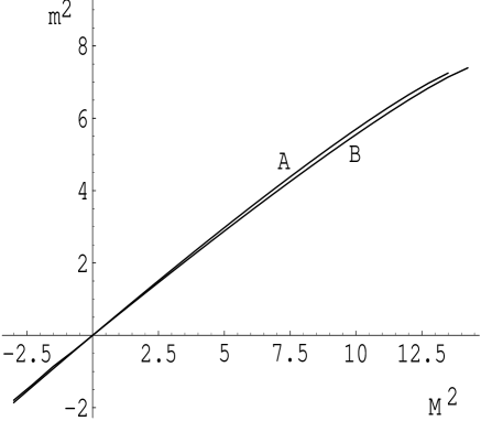
Fig. 2: The solutions $m^{2}$ of $u(z_{0})+4u^{\prime}(z_{0})/(\kappa^{2}\tau)=0$ at chosen values of $M^{2}$ are shown for ($\Lambda>0$, $\mu_{d}=1$) and ($\Lambda<0$, $\mu=1$) by the curves A and B respectively. Here we take $\lambda=10/3$.

For the bound state given above, we should show the normalizability for the localization in the following sense

$$\int_{0}^{y_{H}}dyA^{2}(y)\Phi^{2}(m,y)=\int_{z_{0}}^{\infty}dz~{}u^{2}(m,z)<\infty,$$ (43)

for the bounded-mode solution $u(m,z)$ given above. It is easy to see that this condition is satisfied if $m^{2}<9\lambda/4$, then the solutions are normalizable.

The results for the case of $\lambda>0$ are summarized as follows; For both cases of $\Lambda>0$ and $\Lambda<0$, (i) we can find the bound state in the expected region, $0\leq m<3\sqrt{\lambda}/2$, for positive $M^{2}$. (ii) In the case of $M^{2}<0$, the tachyonic bound state of $m^{2}<0$ appears as presented as in the case of $\lambda=0$ [7]. This point will be important in considering the stability-problem of brane-world.

3.2 Anti de Sitter Brane

In this subsection, we consider the case of AdS brane ($\lambda<0$). Such brane is obviously allowed only for AdS bulk ($\Lambda<0$), because of (7). For the Randall-Sundrum brane ($\lambda=0$), it is known that tachyons can live in AdS₅ bulk with keeping the bulk stable [13]. This property persists also for the AdS brane, as shown later. Thus, three types of particles, massive and massless particles and tachyons, can reside in AdS₅ bulk with AdS₄ brane. We then investigate their localization systematically.

Using $\partial z/\partial y=A^{-1}$ for $A(y)$ of Eq. (14), we obtain a new coordinate $z$ as $z={\rm sgn}(y)\arctan{\{\sinh{\mu(|y|-y_{H})}\}}/H$. Discussions made below are parallel for both cases of positive and negative $y$. We then consider the case of positive $y$ only. As for positive $y$, the potential $V$ in Eq. (24) is

$$V(z)={15\over 4}H^{2}[\frac{\hat{a}}{\cos{{}^{2}(Hz)}}-{3\over 5}]-{\kappa^{2}\tau\over 2}\delta(z-z_{0}),$$ (44)

$$\hat{a}=1+a\,,\qquad a={4M^{2}\over 15\mu^{2}}=-{8M^{2}\over 5\Lambda}\,,\qquad H=\sqrt{-\lambda}\,,\qquad z_{0}=-{1\over H}\arccos({H\over\mu}).$$ (45)

Here $z$ varies in a range $z_{0}\leq z\leq\pi/2H$, and $z_{0}$ is a value of $z$ at $y=0$, indicating the brane resides in $z=z_{0}$. Note that $0\leq\beta\equiv H/\mu\leq 1$ because of Eq. (7). The potential contains a $\delta$-function force with the same form as in the case of dS brane ($\lambda>0$). Hence, the solution of Eq. (24) satisfies the same boundary condition at $z=z_{0}$ as Eq.(42). Again, an attractive $\delta$-function force ($\tau>0$) guarantees that particles are trapped on the brane.

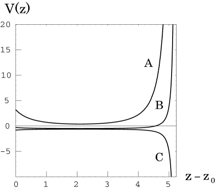
Fig. 3: The $z$ dependence of $V(z)$ in a case of $H=0.5$ and $\mu=1$. Here $z$ varies from $z_{0}=-2.09$ to $z_{1}=\pi$. Three lines A, B, C show the result for $\hat{a}=1,1/15,-1/15$ ($M^{2}=0,-7/2,-4$), respectively.

The analytic part of $V(z)$ depends on $M$ through $\hat{a}$. Three typical cases are shown in Fig. 3. Types (A) and (B) show the part for $\hat{a}=1$ and 1/15, respectively. As for $\hat{a}\geq 0$, thus, the analytic part is divergent at $z=z_{1}$, where $z_{1}=\pi/2H$. All the eigenstates $u(z)$ of Eq.(24) are then bound states satisfying

$$u(z_{1})=0.$$ (46)

On the other hand, Type (C) is the potential for $\hat{a}=-1/15$ corresponding to $M^{2}=-4$. For $\hat{a}<0$, the potential is strongly attractive near $z=z_{1}$. This means that in general the resultant bound state is localized not only near $z=z_{0}$ but also near $z=z_{1}$. Thus, particles can not be trapped only at the brane in this case. We then consider only the case of $\hat{a}\geq 0$, corresponding to $M^{2}\geq-15\mu^{2}/4$.

The analytic part of $V$ has a minimum at $z=0$. It behaves as $V(0)=3H^{2}/2+H^{2}M^{2}/\mu^{2}$. When the eigenvalue $m^{2}$ of Eq.(24) is smaller than the minimum $V(0)$, the corresponding bound state is localized on the brane. When $m^{2}\geq V(0)$, on the other hand, the bound state spreads in the bulk. The mass confined on the brane is then expected in the region

$$m^{2}<V(0).$$ (47)

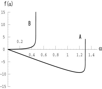
Fig. 4: The $\alpha$ dependence of $f$. Two lines A, B show the result for $\beta=0.5$ and 0.95, respectively.

First, we consider the limit of small $\hat{a}$ and analyze analytically the localization of particles there. This analysis gives a good insight to the localization mechanism for finite $\hat{a}$, as shown later. In the limit, only tachyon can live in the bulk, because $M^{2}<0$ there. Comparing two curves (A) and (B) in Fig. 3, we find that the analytic part of $V$ tends to a well potential: $V(z)=-9H^{2}/4$ for $z_{0}<z<z_{1}$ and $V(z)=\infty$ for $z=z_{1}$. The solution of Eq. (24) then takes the form $u(z)=c_{1}\exp(-\alpha\mu z)+c_{2}\exp(\alpha\mu z)$, where $\alpha^{2}=-(m/\mu)^{2}-9\beta^{2}/4$ and $\beta=H/\mu$. The relation between $\alpha^{2}$ and $m^{2}$ indicates that $\alpha$ is real for the solution to satisfy the trapping condition (47). Imposing two boundary conditions, Eqs. (42) and (46), on the solution, we can determine eigenvalues from Eq. (24). The lowest eigenvalue $m^{2}$, relevant to the localization, satisfies

$$f(\alpha)\equiv\log[{{3\over 2}\sqrt{1-\beta^{2}}+\alpha\over{3\over 2}\sqrt{1-\beta^{2}}-\alpha}]-2\alpha[{\pi\over 2\beta}+{\arccos{(\beta)}\over\beta}]=0.$$ (48)

The equation has a solution $\alpha=0$, but it leads to a trivial solution $u(z)=0$. We then define the left hand side of Eq.(48) as $f(\alpha)$ and investigate the $\alpha$ dependence in order to find out a nontrivial solution. Figure 4 shows the $\alpha$ dependence for two typical cases of $\beta=0.5$ and 0.95. It is found from the figure that there exists a nontrivial solution for $\beta=0.5$, but not for $\beta=0.95$. This is understood, as follows. For any $\beta$, $f(\alpha)$ is zero at $\alpha=0$ and infinity at $\alpha=3\sqrt{1-\beta^{2}}/2$, and the second derivative of $f(\alpha)$ with respect to $\alpha$ is positive in the range $0<\alpha<3\sqrt{1-\beta^{2}}/2$. So, Eq.(48) has a nontrivial solution when $df(\alpha)/d\alpha<0$ at $\alpha=0$, but no solution when $df(\alpha)/d\alpha\geq 0$ at $\alpha=0$. The first derivative of $f$ has a simple form $4/(3\sqrt{1-\beta^{2}})-2\{\pi/(2\beta)+\arccos{(\beta)}/\beta\}$ at $\alpha=0$, and it is negative at $0<\beta<0.9440$ and positive at $0.9440<\beta<1$. Hence, there is a solution satisfying the trapping condition (47) for $0<\beta<0.9440$, but not for $0.9440<\beta<1$. The solution thus found has a negative $m^{2}$ at $M^{2}=-15\mu^{2}/4$. In the limit of small $\hat{a}$, therefore, the tachyon living in the bulk is trapped on the brane as a tachyon, only when $0<\beta<0.9440$.

Next, we analytically investigate the $M^{2}$ dependence of the lowest eigenvalue $m^{2}$. The lowest eigenvalue and the corresponding normalized eigenstate, $u$, satisfy Eq. (20). Differentiating both the sides of the equation with respect to $M^{2}$ leads to

$${dm^{2}\over dM^{2}}=<u|{dV(z)\over dM^{2}}|u>,$$ (49)

since $<du/dM^{2}|u>+<u|du/dM^{2}>=0$ because of $<u|u>=1$. The right hand side of Eq. (49) is easily calculated into $<u(M,z)|{\rm sec}^{2}(Hz)|u(M,z)>H^{2}/\mu^{2}$, and found to be larger than $H^{2}/\mu^{2}$ because of $\cos{(Hz)}\leq 1$ at any $z$ between $z_{0}$ and $z_{1}$. This leads to an relation

$${dm^{2}\over dM^{2}}>{dV(0)\over dM^{2}}={H^{2}\over\mu^{2}}.$$ (50)

As for $0.9440<\beta<1$, the lowest eigenvalue $m^{2}$ is above $V(0)$ at the limit of small $\hat{a}$, as mentioned above. The relation (50) guarantees that $m^{2}>V(0)$ at any positive $\hat{a}$, or at any $M^{2}$ larger than the lower bound $-15\mu^{2}/4$, indicating no localization of particles on the brane at any $M^{2}$. For $0<\beta<0.9440$, on the other hand, $m^{2}$ is below $V(0)$ in the limit of small $\hat{a}$, as mentioned above. As $M^{2}$ increases from the lower bound, $m^{2}$ overtakes $V(0)$ because of the relation (50). Thus, particles are trapped on the brane at least for $M^{2}$ near the lower bound.

For the case of positive $\hat{a}$, the Schrödinger-like equation (24) has a general solution $u(z)=\bar{c}_{1}F(z)+\bar{c}_{2}G(z)$ for

$$F(z)=W^{-id}{}_{2}F_{1}(\bar{b}_{1},\bar{b}_{2};c;W),\quad G(z)=W^{id}{}_{2}F_{1}(\bar{b}_{1}^{\prime},\bar{b}_{2}^{\prime};c^{\prime};W),$$ (51)

where $\bar{c}_{1,2}$ are integration constants and

$$W={1\over{\rm cos}^{2}(Hz)},\quad d={\sqrt{-9-4m^{2}/H^{2}}\over 4}.$$ (52)

Here $(\bar{b}_{1},\bar{b}_{2},c)$ and $(\bar{b}_{1}^{\prime},\bar{b}_{2}^{\prime},c^{\prime})$ are obtainable from $(b_{1},b_{2},c)$ and $(b_{1}^{\prime},b_{2}^{\prime},c^{\prime})$, defined in (38) and (39), by replacing $a_{1}\to-a$. After the replacement, Eqs. (38) and (39) show that $G(z)$ and $F(z)$ are complex conjugate to each other for $M^{2}\geq-4\mu^{2}$, but not for $M^{2}<-4\mu^{2}$. As stated above, it indicates that the ground state of AdS$-5$ bulk is stable only at $M^{2}\geq-4\mu^{2}$. A similar discussion is also possible for AdS brane. The corresponding stability condition for the brane is $m^{2}<9H^{4}/4$.

The eigenmode of Eq.(24) has to satisfy the two boundary conditions, (42) and (46):

$${G^{\prime}(z_{0})+{3\over 2}\sqrt{\mu^{2}-H^{2}}G(z_{0})\over F^{\prime}(z_{0})+{3\over 2}\sqrt{\mu^{2}-H^{2}}F(z_{0})}=\lim_{z\to z_{1}}{G(z)\over F(z)}.$$ (53)

Both $F(z)$ and $G(z)$ are divergent at $z=z_{1}$, although the ratio is finite. As a result of the dangerous behavior of $F(z)$ and $G(z)$ near $z=z_{1}$, it is hard to obtain any eigenmode numerically with Eq. (53). So we solve the Schrödinger-like equation (24) numerically with the Runge-Kutta method which propagates solutions satisfying the initial condition (46) from $z_{1}$ to $z_{0}$. Among numerical solutions, each with different $m^{2}$, eigenmodes are chosen so that the solution can satisfy the boundary condition (42) at $z=z_{0}$.

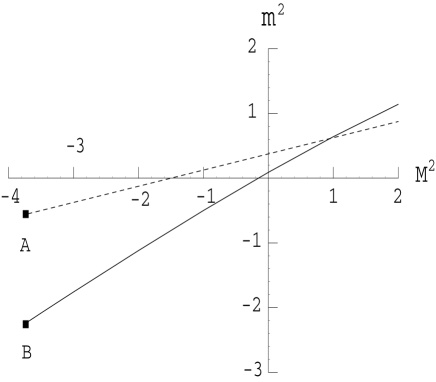
Fig. 5: The lowest eigenvalue $m^{2}$ and the potential minimum $V(0)$ as a function of $M^{2}$. The former is shown by a solid line and the latter is by a dashed one. Points A and B are $V(0)$ and $m^{2}$ in the limit of $\hat{a}\to 0$. Parameters taken are $\mu=1$ and $\beta=H/\mu=0.5$.

Figure 5 shows the resulting lowest eigenvalue $m^{2}$ as a function of $M^{2}$. Here we take $\mu=1$ and $\beta=H/\mu=0.5$, as an example of $\beta$ belonging to the region $0<\beta<0.9440$. Points A and B stand for $V(0)$ and $m^{2}$, respectively, at $M^{2}=-3.75$ corresponding to the limit of $\hat{a}\to 0$. As expected, $m^{2}$ is below $V(0)$ there. As $M^{2}$ is increased from the lower bound, $m^{2}$ catches up with $V(0)$ at $M^{2}=0.95$. Thus, tachyons and massless and massive particles are confined in the brane when $-3.75<M^{2}<0.95$. At $-0.15<M^{2}<0$, especially, a tachyon is trapped on the brane as either a massless or massive particle. The resultant $M^{2}$ dependence of $m^{2}$ is a simple form $m^{2}=c_{1}+c_{2}M^{2}$, where $c_{i}$ are positive. A graviton with $M^{2}=0$ is confined as a massive particle with small $m^{2}=c_{1}$. This is consistent with the previous analyses on graviton [11]. As for $0.9440<\beta<1$, on the other hand, numerical calculations shows no localization of particles at any $M^{2}$, as expected.

4 Concluding remarks

We have examined the localization of massive scalar on both dS and AdS branes, where mass $M$ of scalar particle is varied from the massless- and massive-particle region $M^{2}\geq 0$ to the tachyonic region $M^{2}<0$. As a bulk space, we consider both cases, AdS₅ and dS₅. The dS₅ bulk, with positive 5d cosmological constant ($\Lambda>0$), has recently attracted interest in connection with the proposed dS/QFT correspondence [14]. The AdS₅ bulk is not only interested in the context of AdS/CFT correspondence, but also important in the sense that the bulk is derivable from superstring through the dimensional reduction. As a characteristic of AdS₅ bulk, it is found that the ground state of the bulk is stable only when $M^{2}\geq-4|\Lambda|/6$, independently of brane, for both dS and AdS branes. Thus, even tachyons can reside in AdS bulk, with keeping the vacuum stable, when $M^{2}\geq-4|\Lambda|/6$.

As for dS brane, with positive 4d cosmological constant ($\lambda>0$), the continuous KK modes of scalar fluctuation are found in the mass range $m^{2}>9\lambda/4$, for both AdS₅ and dS₅ bulks. The mass gap for the KK modes is a characteristic of dS brane.

For such dS brane, massive scalar is localized on the brane as a massive mode. A mass $m$ of the mode is related to $M$ as $m^{2}=cM^{2}$ for a calculable positive constant $c$, when $m^{2}\ll|\Lambda|$. The localized mode has to be found in the mass gap, so massive scalar can be localized on dS brane only when $M^{2}<9\lambda/4c$. In the case of the Randall-Sundrum brane with $\lambda=0$, on the other hand, there is no mass gap for the continuous KK modes, so that any massive scalar can not be localized on the brane.

As for AdS brane, which is allowed only for AdS₅ bulk, massive scalar with $M^{2}>0$ is also localized on the brane as a massive mode, and the localized mode is related to $M^{2}$ as $m^{2}=c_{1}M^{2}+c_{2}$ for positive constants $c_{i}$. In the limit of small $M^{2}$, the formula shows that graviton is trapped on AdS brane as a massive particle [11].

Extending the analyses mentioned above to negative $M^{2}$, we can find tachyonic ($m^{2}<0$) localized modes, for both cases of dS and AdS branes. The relation of the mode to $M^{2}$ is the same as in the case of massive mode: $m^{2}=cM^{2}$ for dS brane and $m^{2}=c_{1}M^{2}+c_{2}$ for AdS brane. Furthermore, it is found that the ground state of brane is stable at $m^{2}>0$ for the case of dS brane and at $m^{2}>-9|\lambda|/4$ for the case of AdS brane.

As for dS brane embedded in AdS₅ bulk, the formula on $m^{2}$ shows that once tachyons exist in the bulk, the tachyonic mode also appears on the brane and makes the brane unstable. In this sense, tachyons can not exist in AdS₅ bulk. For AdS brane embedded in AdS₅ bulk, on the other hand, the formula on $m^{2}$ shows a possibility that tachyons are trapped on the brane as either a massless or massive mode, but graviton is not localized on the AdS brane as a massless mode. Therefore, we can conclude that tachyons should be prohibited in AdS₅ bulk for both cases of AdS and dS branes. It is quite an interesting issue why and how tachyons are prohibited when the five-dimensional theory is reduced from superstring.

As a natural statement, we can say that the observed acceleration of the present universe is induced by small positive $\lambda$. At the same time, it is expected from the recent observations that some amount of cold dark matter coexists with the cosmological constant. The coexistence would be explainable from the brane-world viewpoint. If a small but finite $\lambda$ exists, massive scalar living in the bulk can be trapped on the present universe as a massive mode, when $m<3\sqrt{\lambda}/2\sim 10^{-3}$ eV. The trapped particles are so called ‘dark’ in the sense that they interact with ordinary matters on the brane only through gravitation. As a result of the weak interaction, it is likely that the trapped particles are also ‘cold’ in the sense that they are hardly thermalized. Thus, this scalar could be a candidate for the cold dark matter. As an important fact, it should be stressed that the coexistence occurs only when the positive cosmological constant exists.

References

- [1] L. Randall and R. Sundrum, Phys. Rev. Lett. 83 (1999) 3370, (hep-ph/9905221).
- [2] L. Randall and R. Sundrum, Phys. Rev. Lett. 83 (1999) 4690, (hep-th/9906064).
- [3] I. Brevik, K. Ghoroku, S. D. Odintsov and M. Yahiro, Phys. Rev. 66 (2002) 064016, (hep-th/0204066). B. Bajc and G. Gabadadze, Phys. Lett. B474 (2000) 282, (hep-th/9912232). M. Ito, (hep-th/0204113). P. Singh and N. Dadhich, (hep-th/0208080).
- [4] N. Arkani-Hamed, S. Dimopoulos, N. Kaloper and R. Sundrum, Phys. Lett. B480 (2000) 193, (hep-th/0001197).
- [5] S. Kachru, M. Schulz and E. Silverstein, Phys. Rev. D62 (2000) 045021, (hep-th/0001206).
- [6] K. Ghoroku, and M. Yahiro, to be published in Phys. Rev. D (hep-th/0206128).
- [7] K. Ghoroku, and A. Nakamura, Phys. Rev. D64 (2001) 084028, (hep-th/0103071).
- [8] M. Pernici, K. Pilch and P. van Nuiuwenhuizen, Nucl. Phys. B259 (1985) 460.
- [9] K. Behrndt and M. Cvetic, Phys. Rev. D61 (2000) 101901, (hep-th/0001159).
- [10] S.L. Dubovski, V.A. Rubakov and P.G. Tinyakov, Phys. Rev. D62 (2000) 105011, (hep-th/0006046).
- [11] A. Karch and L. Randall, JHEP 0105 (2001) 008, (hep-th/0011156).
- [12] A. Miemiec, hep-th/0011160.
- [13] P. Breitenlohner and D.Z. Freedman, Ann. Phys. 144 (1982) 249; Phys. Lett. B115 (1982) 197.
- [14] S. Nojiri and S. D. Odintov, hep-th/0107134.