Duke-CGTP-02-09

hep-th/0211110

Blocking up D-branes :
Matrix Renormalization ?

K. Narayan

Center for Geometry and Theoretical Physics,
Duke University,
Durham, NC 27708.
Email : narayan@cgtp.duke.edu

Drawing analogies with block spin techniques used to study continuum limits in critical phenomena, we attempt to block up D-branes by averaging over near neighbour elements of their (in general noncommuting) matrix coordinates, i.e. in a low energy description. We show that various D-brane (noncommutative) geometries arising in string theory appear to behave sensibly under blocking up, given certain key assumptions in particular involving gauge invariance. In particular, the (gauge-fixed) noncommutative plane, fuzzy sphere and torus exhibit a self-similar structure under blocking up, if some “counterterm” matrices are added to the resulting block-algebras. Applying these techniques to matrix representations of more general D-brane configurations, we find that blocking up averages over far-off-diagonal matrix elements and brings them in towards the diagonal, so that the matrices become “less off-diagonal” under this process. We describe heuristic scaling relations for the matrix elements under this process. Further, we show that blocking up does not appear to exhibit any “chaotic” behaviour, suggesting that there is sensible physics underlying such a matrix coarse-graining. We also discuss briefly interrelations of these ideas with B-fields and noncommutativity.

1 The basic ideas and motivations

Noncommutative geometry arises in various situations in string theory [1]. In particular, the low energy dynamics of D-branes stems from the low lying fluctuations of open strings stretched between them. This gives rise to nonabelian gauge theories with charged scalar fields that describe transverse fluctuations of the D-brane worldvolumes as well as other matter fields. Various D-brane configurations are then described in terms of a set of commutation relations among the scalars (regarded here as matrices)

$$[X^{i},X^{j}]=i\theta^{ij}(X)$$ (1)

$\theta^{ij}(X)$ is an antisymmetric 2-form that in general depends on the coordinate variables $X^{i}$ (we restrict attention here to spatial noncommutativity, i.e. $\theta^{0i}=0$). When the $X^{i}$ commute with each other, i.e. $\theta^{ij}=0$, the eigenvalues of the matrices $X^{i}$ can be interpreted as spacetime coordinates describing the positions of the D-branes. However, in general, the coordinate variables $X^{i}$ do not commute so that “points” on the space (1) cannot be specified with arbitrary accuracy. This gives rise to a geometry defined by noncommuting matrices [2]. In e.g., the construction [3] of BPS states in Matrix theory [4] (see also [5]), or the Myers dielectric effect [6], the space (1) can be interpreted as a higher dimensional brane.

Whenever the coordinate variables $X^{i}$ do not commute, there are operator ordering ambiguities in defining observables as functions of these noncommuting coordinates. On the other hand, there are no such ambiguities in defining the corresponding function in the commutative limiting geometry. In general, several classes of functions on the noncommutative geometry collapse onto the same function in the commutative limit. Thus various noncommuting observables on a given noncommutative geometry reduce to the same commutative observable. In this sense, the commutative description is a smooth coarse-grained approximation to the underlying microscopic D-brane description – the noncommutative description contains more information than the commutative approximation.

Thinking thus of the commutative limit as a coarse-grained or averaged approximation to the underlying noncommutative background is reminiscent of, e.g. thinking of a continuum field theory as a coarse-grained smooth approximation to a spin system near a critical point, or a lattice gauge theory – the underlying lattice structure is the microscopic description but near the critical point, there are long range correlations and one can block up spins to define effective lattice descriptions iteratively and thereby move towards the continuum limit [14]. Thus it is tempting to ask if one can apply similar ideas and “block up D-branes” by averaging over nearest neighbour open string modes at the level of matrix variables, thereby moving towards the commutative limit. In what follows, we show that these ideas do indeed lead to interesting physics.

It is important to note that since gauge transformations cannot undo the noncommutativity, this means that off-diagonal open string modes necessarily have nonzero vevs in such a configuration. A specific solution to (1) can be expressed in terms of a set of representation matrices with necessarily nonzero off-diagonal matrix elements. Since the off-diagonal modes in general have nonzero vevs, it is plausible to think of the resulting noncommutative geometry as a condensate of the underlying D-brane (and therefore open string) degrees of freedom that build up the geometry, as outlined previously. Thinking of the noncommutative geometry as akin to a condensed matter system near a critical point, it is tempting to think of the open string modes as developing “long range correlations”, leading to a condensation of some of the modes. For example, as a lattice spin system approaches its critical point, long range correlations develop and patches of correlated spins emerge. One can then block up the underlying microscopic spin degrees of freedom to construct effective block spin degrees of freedom, as in the Kadanoff scaling picture [14]. Holding the block spins fixed and averaging over the microscopic spins yields a new theory describing the interactions of these block spins, with new parameters that have been scaled appropriately to reflect the block transformation.

We would like to take these ideas almost literally over to D-brane matrix variables, where we then proceed to average over “nearest neighbour” open string modes to generate effective D-brane geometries. We define block D-branes at the level of the effective low energy description by averaging over nearest neighbour matrix elements to define new matrix representations of (1) and thus a blocked-up or averaged background. The new matrix representations generated under blocking up have “renormalized” matrix elements. For the noncommutative 2-plane, we hold the distances between points in the commutative limiting 2-plane fixed as we block up – this preserves the translation isometries of the 2-plane. Iterating the matrix blocking procedure moves towards progressively more coarse-grained descriptions. Blocking up in this fashion turns out to shrink the off-diagonal modes thus reducing the noncommutativity. In general, blocking up brings far-off-diagonal modes in, towards the diagonal. The matrices become “less off-diagonal” in the sense that if initially they satisfy the scaling relation $\ X_{ab}\sim X_{aa}\ q^{|b-a|}\$ for some $q<1$, then the resulting block-matrices satisfy a similar relation with ${\tilde{q}}\sim q^{2}((1+q)/2q)^{1/(b-a)}$, showing that far-off-diagonal modes scale away fast relative to the near-off-diagonal ones. We find nontrivial conditions on the scalar matrix elements for blocking up to move towards a commutative limit. Furthermore, we find that blocking up does not seem to exhibit any “chaotic” behaviour, thus indicating that there is sensible physics underlying such a matrix coarse-graining.

In this work, we make the nontrivial assumption that gauge invariance has been fixed to yield a set of matrices that are best suited to recovering a commutative limit. This turns out to be equivalent to assuming that the matrix elements are ordered in specific ways. Physically this essentially picks a convenient gauge in which D-brane locations at the level of matrix variables are in some sense identified with D-brane locations in physical space. The interesting (and more difficult) question of what the gauge-invariant physical matrix coarse-graining is, that this work is a gauge-fixed version of, will be left for the future.

Roughly speaking, one expects a smooth space only if one pixellates the space using small enough pixels, in other words, a large number of “points” or D-branes. Thus in general, one expects that any such block brane techniques would only make sense in a large $N$ limit (see for e.g. [15] for a worldsheet description of D-branes on a fuzzy sphere). It is also useful to recall the ideas of deconstruction [16] where certain quiver theories (in some regions of the moduli space) can be thought of as developing extra dimensions which are the quiver space, so that in some sense D-brane positions are identified with lattice sites in the deconstructed dimensions. At low energies, the effective theory does not see the fact that the extra dimensions are really lattice-like and a continuum description emerges.

Some words on the organization of this work : Sec. 2 lays out the basic definitions while Sec. 3 analyzes the noncommutative plane detailing the consequences of blocking up and the commutative limit, outlining possible interrelations with noncommutative field theories and finally the role of gauge invariance. Sec. 4 studies other nonabelian geometries under blocking up. Sec. 5 studies some general properties of matrices and noncommutative algebras under blocking up. Sec. 6 describes some conclusions and speculations. Finally, appendix A describes the commutative case and appendix B describes an alternative way to block up D-branes and matrices.

Figure 1: Blocking up elements of the original matrix to get a new matrix ($2\times 2$ blocks shown).

2 Blocking up D-branes and matrices : definitions

The scalars $X^{i}$ are hermitian matrices in the adjoint representation of the gauge group, which we take for concreteness to be $U(N)$ for the present. $N$ is assumed to be essentially infinite. Thus the $X^{i}$ satisfy

$$X^{i}_{a,b}={X^{i}}^{{\dagger}}_{a,b}={X^{i}}^{*}_{b,a},\qquad\qquad\qquad a,b=1\ldots N$$ (2)

Define a blocked up matrix as

$${\tilde{X}}^{i}_{a,b}=\alpha(X^{i}_{2a-1,2b-1}+X^{i}_{2a,2b-1}+X^{i}_{2a-1,2b}+X^{i}_{2a,2b}),\qquad\qquad a,b=1\ldots{N\over 2}$$ (3)

In other words, define a matrix entry in the blocked up matrix by averaging over the nearest neighbour matrix entries in $2\times 2$ blocks of the original matrix. This is easier to see pictorially (see figure 1).

The overall factor $\alpha$ has been put in as the normalization constant for uniform averaging. We expect that a uniform normalization constant means that we have averaged uniformly all over the matrix. If we demand that the identity matrix is preserved under blocking up, i.e. ${\bf 1}\rightarrow{\bf 1}$, it is clear that for $2\times 2$ blocks, we must fix $\ \alpha={1\over 2}$. In general, we note that the averaging constant can be different for different matrices, i.e. $\alpha=\alpha^{i}$.

It is clear from the definition of blocking (3) that this preserves hermiticity – the ${\tilde{X}}^{i}$s are also hermitian, so that they are also interpretable as scalars in the adjoint representation of a gauge group. Further, it is also clear that blocking up is (pictorially) symmetric about the diagonal. One would further guess that blocking up in this fashion would average far-off-diagonal modes and bring them in, towards the diagonal. This turns out to be almost (but not quite) true, as we shall see in section 4.

Finally note the following analogy with spin systems near a critical point : defining block spins by averaging over $k\times k$ blocks instead of $2\times 2$ blocks does not change the physics, yielding the same Wilson renormalization group equations. This independence of the block size reflects long range correlations in the system. We expect that if the noncommutative geometry at hand is truly a “condensate” exhibiting long range correlations, defining block D-branes by averaging over blocks of varying sizes should not change the physics. In the examples that follow, we shall see that this is indeed the case. Note that to preserve the identity matrix under $k\times k$ blocks, i.e. ${\bf 1}\rightarrow{\bf 1}$, we must fix $\ \alpha={1\over k}$.

A priori, it is not at all obvious that blocking up matrices in this fashion is a sensible thing to do and if it will lead to any tractable physics. We will see in what follows that it in fact does, if certain key assumptions are made – in particular, we fix gauge invariance and identify D-brane locations at the level of matrix variables with D-brane locations in physical space. This gauge fixing enables remarkable simplifications and leads to recognizable structures which can then be interpreted in a relatively straighforward fashion. This nearest neighbour matrix element averaging is analogous to real space renormalization group methods in critical phenomena and so is perhaps expected to have all the weaknesses of those techniques. A more elegant renormalization group formulation of such a decimation analogous to integrating out thin momentum shells is lacking at this time.

3 $\theta^{ij}=constant$ : the noncommutative plane

The algebra representing the noncommutative or quantum plane is

$$[X^{1},X^{2}]=i\theta^{12}{\bf 1}$$ (4)

Such algebras arise in the construction [3] of infinite BPS branes in Matrix theory [4] where the brane worldvolume coordinates $X^{1},X^{2}$ are noncommutative while the rest commute. It is also the algebra of open string vertex operators on a D-brane boundary, in the presence of a constant $B_{NSNS}$-field [1]. $\theta^{12}$ is inversely proportional to $B_{NSNS}$ in the Seiberg-Witten limit [10]. This algebra is preserved under translations by two independent matrices proportional to the identity matrix

$$(X^{1}_{0},X^{2}_{0})\rightarrow(X^{1}_{0},X^{2}_{0})+(x^{1}{\bf 1},x^{2}{\bf 1}),$$ (5)

where $(X^{1},X^{2})$ is really a “matrix point” defined with a resolution size – thus the algebra defines a two-plane. Using a representation in terms of harmonic oscillator creation/annihilation operators satisfying $\ [a,a^{{\dagger}}]={\bf 1},\$ we can write the $X^{i}$ as

$$X^{1}=x^{1}{\bf 1}+\sqrt{\theta^{12}}{1\over\sqrt{2}}(a+a^{{\dagger}}),\qquad X^{2}=x^{2}{\bf 1}+\sqrt{\theta^{12}}{i\over\sqrt{2}}(-a+a^{{\dagger}})$$ (6)

where $(x^{1},x^{2})$ label a commutative point on the 2-plane. This is thus a decomposition into a “center-of-mass” piece and an off-diagonal piece independent of the location. Thus, in this representation, it seems reasonable to interpret the noncommutative plane as a fuzzy resolution of the commutative plane – at each point $(x^{1},x^{2})$ of the commutative limit, we have a “fuzzy blowup” in terms of noncommuting matrices defining a characteristic pixellation size $\theta^{12}$.

3.1 Blocking up

We would like to preserve the translation isometries (5) of the 2-plane under blocking up. These translations are generated by the identity matrix ${\bf 1}$. Further the commutative “point” is $(x^{1}{\bf 1},x^{2}{\bf 1})$ which we hold fixed under blocking up. This requires that we set the averaging constant $\alpha={1\over 2}$.
Using the convenient basis of energy eigenstates of the harmonic oscillator, we have for the representation matrices of $a,a^{{\dagger}}$,

$$\qquad\qquad\qquad N|n\rangle=a^{{\dagger}}a|n\rangle=n|n\rangle,$$

$$\langle n^{\prime}|a|n\rangle=\sqrt{n}\ \langle n^{\prime}|n-1\rangle=\sqrt{n}\ \delta_{n^{\prime},n-1},\qquad\qquad\langle n^{\prime}|a^{{\dagger}}|n\rangle=\sqrt{n+1}\ \delta_{n^{\prime},n+1}$$ (7)

Let us order the states as

$$|0\rangle=(1,0,0,\ldots)^{T},\ \qquad|1\rangle=(0,1,0,\ldots)^{T},\ \qquad|2\rangle=(0,0,1,0,\ldots)^{T},\ \ldots\\$$

With this basis, we get for the representation matrices of $X^{1}$

$$X^{1}=x^{1}{\bf 1}+\sqrt{\theta^{12}\over 2}\left(\begin{array}[]{cccccccc}0&1&0&0&&&&\ldots\\ 1&0&\sqrt{2}&0&&&&\ldots\\ 0&\sqrt{2}&0&\sqrt{3}&0&&&\ldots\\ 0&0&\sqrt{3}&0&\sqrt{4}&0&&\ldots\\ &&0&\sqrt{4}&0&\sqrt{5}&0&\\ &&&&\sqrt{5}&0&\sqrt{6}&\\ &&&&.&&&\\ &&&&.&&&\\ \end{array}\right)$$ (16)

the representation matrix for $X^{2}$ being easily constructed. Blocking up this matrix in the way defined in the previous section gives

$$X^{1} \rightarrow x^{1}{\bf 1}+{1\over 2}\sqrt{\theta^{12}\over 2}\left(\begin{array}[]{cccccc}2&\sqrt{2}&0&0&&\ldots\\ \sqrt{2}&2\sqrt{3}&\sqrt{4}&0&&\ldots\\ 0&\sqrt{4}&2\sqrt{5}&\sqrt{6}&0&\ldots\\ 0&0&\sqrt{6}&2\sqrt{7}&\sqrt{8}&\ldots\\ &&0&\sqrt{8}&2\sqrt{9}&\ldots\\ &&&&0&\\ &&&.&&\\ &&&.&&\\ \end{array}\right)$$ (25)

$$= x^{1}{\bf 1}+\sqrt{\theta^{12}\over 2}\left(\begin{array}[]{cccccc}1&0&0&0&&\ldots\\ 0&\sqrt{3}&0&0&&\ldots\\ 0&0&\sqrt{5}&0&&\ldots\\ 0&0&0&\sqrt{7}&&\ldots\\ &&&.&&\\ &&&.&&\\ &&&.&&\\ &&&.&&\\ \end{array}\right)+{\sqrt{2}\over 2}\sqrt{\theta^{12}\over 2}\left(\begin{array}[]{cccccc}0&1&0&0&&\ldots\\ 1&0&\sqrt{2}&0&&\ldots\\ 0&\sqrt{2}&0&\sqrt{3}&&\ldots\\ 0&0&\sqrt{3}&0&&\ldots\\ &&0&\sqrt{4}&&\\ &&&.&&\\ &&&.&&\\ &&&.&&\\ \end{array}\right)$$ (42)

In the last line, we have separated the diagonal matrix from the off-diagonal one. Blocking up works in a very similar fashion for $X^{2}$, with the diagonal matrix generated having zero entries. Thus under blocking up,

$${\tilde{X}}^{1} = x^{1}{\bf 1}+\sqrt{\theta^{12}\over 2}D^{1}+{1\over\sqrt{2}}\sqrt{\theta_{12}\over 2}\ (a+a^{{\dagger}}),$$

$${\tilde{X}}^{2} = x^{2}{\bf 1}+\sqrt{\theta^{12}\over 2}D^{2}+{1\over\sqrt{2}}\sqrt{\theta^{12}\over 2}\ i(-a+a^{{\dagger}}),$$ (45)

where the $D^{i}$ are the diagonal matrices that were generated ($D^{2}=0$). Recall that we have held the commutative coordinates $(x^{1}{\bf 1},x^{2}{\bf 1})$ and the translation isometries fixed (by setting $\alpha={1\over 2}$) – thus distances between points $(x^{1}{\bf 1},x^{2}{\bf 1})$ are also held fixed as we block up. The algebra of the new coordinates is

$$[{\tilde{X}}^{1},{\tilde{X}}^{2}]=i{\theta^{12}\over 2}{\bf 1}+\Delta\theta^{12}$$ (46)

where

$$\Delta\theta^{12}={\sqrt{2}\over 2}\theta^{12}\biggl{(}[D^{1},{1\over\sqrt{2}}(-a+a^{{\dagger}})]\biggr{)}$$ (47)

are nonzero since the diagonal matrices $D^{i}$ do not in general commute with an arbitrary matrix (the terms involving $D^{2}=0$ vanish). We will suggestively call the $D^{i}$ “counterterm” matrices. Thus the algebra of the new noncommutative coordinates is “self-similar” in form under blocking up, modulo counterterms involving the diagonal matrices generated under blocking up. Notice further that the new $\theta^{12}$ is scaled down by a factor of $2$. Continuing this blocking up procedure, after $n$ iterations, we have

$$X^{1{(n)}} = x^{1}{\bf 1}+\sqrt{\theta^{12}\over 2}D^{1{(n)}}+{1\over 2^{n/2}}\sqrt{\theta^{12}\over 2}\ (a+a^{{\dagger}})\equiv x^{1}{\bf 1}+\sqrt{\theta^{12}\over 2}D^{1{(n)}}+\lambda(a+a^{{\dagger}})$$

$$X^{2{(n)}} = x^{2}{\bf 1}+\sqrt{\theta^{12}\over 2}D^{2{(n)}}+{1\over 2^{n/2}}\sqrt{\theta^{12}\over 2}\ i(-a+a^{{\dagger}})\equiv x^{2}{\bf 1}+i\lambda(-a+a^{{\dagger}})$$ (48)

where $\ \lambda\sim{1\over 2^{n/2}}\$ is the scaling-down factor and the $kk$th-diagonal element of the $D^{1{(n)}}$ is

$${D^{1{(n)}}}_{kk}={1\over 2^{n-1}}\biggl{(}\sqrt{2^{n}.(k-1)+1}+\sqrt{2^{n}.(k-1)+2}+\ldots+\sqrt{2^{n}.(k)-1}\biggr{)}$$ (49)

There are $2^{n}.(k)-2^{n}.(k-1)-1=2^{n}-1$ terms inside the bracket, so that the diagonal elements ${D^{1{(n)}}}_{kk}$ do not shrink to zero along with the off-diagonal elements. Indeed

$$lim_{n\rightarrow\infty}\ {D^{1{(n)}}}_{kk}\sim 2^{(n+2)/2}\sqrt{k}\neq 0$$ (50)

so that blocking up does not scale down the diagonal elements of $D^{1}$, while scaling down the off-diagonal ones ($D^{2}=0$). The algebra of the new coordinates after $n$ iterations is

$$[{\tilde{X}}^{1},{\tilde{X}}^{2}]=i{\theta^{12}\over 2^{n}}{\bf 1}+\Delta\theta^{12}$$ (51)

where the counterterms are

$$\Delta\theta^{12}={1\over 2^{n/2}}\theta^{12}\biggl{(}[D^{1{(n)}},{1\over\sqrt{2}}(-a+a^{{\dagger}})]\biggr{)}$$ (52)

We see from (51) that $\theta^{12}$ shrinks exponentially with each iteration while the commutative coordinates are held fixed. Thus the limit of the blocking up transformation is $\theta^{12}=0$.

Averaging over $3\times 3$ blocks, say, or larger blocks turns out to be equivalent to averaging over $2\times 2$ blocks. Indeed, averaging uniformly over $k\times k$ blocks, we see a periodic repetition of off-diagonal blocks involving factors of $\sqrt{k}$ which thus exhibits a self-similar structure like the one above with $2\times 2$ blocks. Thus we find that the new noncommutative pieces of the coordinates scale after $n$ iterations as $a\rightarrow\biggl{(}{\sqrt{k}\over k}\biggr{)}^{n}a,\ \ a^{{\dagger}}\rightarrow\biggl{(}{\sqrt{k}\over k}\biggr{)}^{n}a^{{\dagger}}$ after subtracting the diagonal matrices, so that $\theta^{12}$ shrinks as

$$\theta^{12}\rightarrow\theta^{12}\ {1\over k^{n}}$$ (53)

thus shrinking noncommutativity. This is again reassuring, since if indeed such a D-brane configuration is a “condensate” with long-range correlations, blocking up the constituents into blocks of different sizes should not change the essential physics. In what follows, we stick to $2\times 2$ blocks.

3.2 The commutative limit : matrix renormalization ?

Consider now an arbitrary function of the noncommutative plane coordinates (3.1), (3.1) that has a matrix Taylor expansion

$$f({\tilde{X}}^{1},{\tilde{X}}^{2})=\sum_{a_{m}}f_{a_{1}a_{2}\ldots a_{m}}\ {\tilde{X}}^{a_{1}}{\tilde{X}}^{a_{2}}\ldots{\tilde{X}}^{a_{m}},\qquad\qquad a_{i}=1,2$$ (54)

There are operator ordering ambiguities in such an expansion for any nonzero $\lambda\sim\alpha^{n/2}={1\over 2^{n/2}}$, $\alpha$ being the averaging constant, since ${\tilde{X}}^{1}$ and ${\tilde{X}}^{2}$ do not commute. With successive blocking up iterations, $\lambda$ shrinks. Thus the above expansion collapses as $\lambda\rightarrow 0$ to

$$f = \sum_{a_{m}}f_{a_{1}a_{2}\ldots a_{m}}\ ({x^{a_{1}}{\bf 1}+D^{a_{1}}})\ ({x^{a_{2}}{\bf 1}+D^{a_{2}}})\ \ldots\ ({x^{a_{m}}{\bf 1}+D^{a_{m}}})$$

$$\rightarrow \sum_{m,n}F_{mn}(x^{1}{\bf 1}+D^{1})^{m}(x^{2}{\bf 1}+D^{2})^{n}=f\biggl{(}(x^{1}{\bf 1}+D^{1}),(x^{2}{\bf 1}+D^{2})\biggr{)}$$

$$= f(X^{1},X^{2})|_{\rm commutative}$$ (56)

since the diagonal matrices $(x^{i}{\bf 1}+D^{i})$ commute with each other. Thus any well-behaved function asymptotes to the commutative restriction of the function in the limit of blocking up ad infinitum.
Further the distance between points $P^{k}=(x^{k1}{\bf 1}+D^{1},x^{k2}{\bf 1}+D^{2})$ is

$$d_{P^{a},P^{b}}=|(x^{a1}{\bf 1}+D^{1}-x^{b1}{\bf 1}-D^{1})^{2}+(x^{a2}{\bf 1}+D^{2}-x^{b2}{\bf 1}-D^{2})^{2}|^{1/2}\equiv|{\vec{x}}^{a}-{\vec{x}}^{b}|,$$ (57)

i.e. the $D^{i}$ do not show up in the distances between points in the commutative limiting space.
Thus it appears that we cannot really tell the difference between $(x^{1})$, $(x^{1}{\bf 1})$ and $(x^{1}{\bf 1}+D^{1})$ in the commutative limit, insofar as functions with a matrix-Taylor expansion are concerned since they all collapse down to expressions involving purely commuting quantities. In other words, if we replace $(x^{i}{\bf 1}+D^{i})$ by $(x^{i}{\bf 1})$, the functional expression (54), (3.2) does not appear to change in the limit of an infinite number of iterations, i.e. from the point of view of the limiting commuting matrices. It is thus interesting to ask if the $D^{i}$ are observable at all and if one can formally define new commuting coordinates by shifting away the diagonal matrices $D^{i}$. This is essentially equivalent to formally subtracting off the diagonal matrices $D^{i}$ and thus the counterterms $\Delta\theta^{12}$ as well. This is a $\theta$-dependent “renormalization” of the commutative matrix coordinates. Recall that the $D^{i}$ are diagonal matrices with diverging entries in the limit of infinite blocking up iterations. If this shift by an infinite diagonal matrix is not observable, this redefinition in terms of new commuting coordinates $(x^{i}{\bf 1})$ would be legal. The diagonal matrices $D^{i}$ generated reflect the fact that we have lost information in averaging. The above matrix “renormalization” then means that we have added new counterterms that simulate the effects of averaging over short distance open string modes to cancel the generated counterterms, in much the same way as counterterms in field theory generated on changes of an ultraviolet cutoff reflect short distance physics that has been integrated out.
The key physical question is to understand what physical observables are represented by these classes of matrix functions where shifting away the $D^{i}$ is legitimate after blocking up. In other words, when shifting away the $D^{i}$ is observable. For instance, it is not clear if shifting by the $D^{i}$ is legal at each iteration order. At any finite iteration order, we have not averaged over all the constituent D0-branes at any point of the 2-brane condensate so there is a physical difference between the $(x^{i}{\bf 1}+D^{i})$ since for example,

$$(x^{i}{\bf 1}+D^{i})_{nn}-(x^{i}{\bf 1}+D^{i})_{n^{\prime}n^{\prime}}=(D^{i})_{nn}-(D^{i})_{n^{\prime}n^{\prime}}\neq 0$$ (58)

corresponds, in some sense, to the difference in locations of the $n$ and $n^{\prime}$ 0-branes at the point $(x^{1}{\bf 1},x^{2}{\bf 1})$. Thus differences in the $D^{i}$ elements are visible at a finite iteration order. This is reminiscent of divergent sums of zero point energies in free field theory – they are unobservable in empty space but do have observable consequences in the presence of boundaries as in the Casimir effect for instance. It is interesting to look for Casimir-effect-like thought experiments where differences (58) in the $D^{i}$s might be observable.
To summarize, we have found that the off-diagonal parts of the algebra after blocking up are self-similar with reduced noncommutativity parameter if we subtract off certain “counterterm” matrices which cancel the $D^{i}$ matrices. [31] describes a block-spin-like transformation on some classes of orbifold quiver gauge theories obtained by sequentially Higgsing the gauge symmetry in them, thereby performing a sequence of partial blowups of the orbifolds. It is interesting to note that subtracting a similar set of diagonal matrices after coarse-graining the “upstairs” matrices of the “image” branes in the $C^{2}/Z_{N}$ quiver reproduces the worldvolume Higgsing that partially blow-up the geometry into a $C^{2}/Z_{N/2}$ quiver [31]. More generally in the other $C^{3}/Z_{N}$ quivers considered there, the “counterterm” matrices required to be subtracted correspond to fields that become massive under the Higgsing. Thus perhaps such “counterterm” matrices are expected in general to make sense of this matrix coarse-graining.
Let us now consider multiplication of two (noncommuting) operators ${\cal O}_{f}$ and ${\cal O}_{g}$ on the noncommutative plane corresponding to (commuting) functions $f(x)$ and $g(x)$ in the commutative limit. The operators can be defined as

$${\cal O}_{f}(X)={1\over(2\pi)^{2}}\int d^{2}k\ {\tilde{f}}(k)e^{-ik\cdot X}$$ (59)

where the $X$ are noncommuting coordinates satisfying (4) and $\ {\tilde{f}}(k)=\int d^{2}x\ f(x)e^{ik\cdot x}\$ is the Fourier transform of the (commutative) function $f(x)$. Then we have ${\cal O}_{f}\cdot{\cal O}_{g}={\cal O}_{f*g}$, where $*$ is the usual associative Moyal product that gives

$$f*g(x) \equiv e^{{i\over 2}\theta^{\mu\nu}\partial_{\mu}^{y}\partial_{\nu}^{z}}f(y)g(z)\bigg{|}_{y=z=x}=f(x)g(x)+{i\over 4}\theta^{\mu\nu}(\partial_{\mu}f\partial_{\nu}g-\partial_{\nu}f\partial_{\mu}g)+{\cal O}(\theta^{2})$$ (60)

$$= \int d^{2}k\ d^{2}k^{\prime}\ {\tilde{f}}(k){\tilde{g}}(k^{\prime}-k)\ e^{-ik^{\prime}\cdot x}\ e^{-{i\over 2}\theta^{\mu\nu}k_{\mu}k^{\prime}_{\nu}}$$

Under blocking up, we generate new noncommuting coordinates (3.1), (3.1) so that the new operators become

$${\cal O}_{f}=\int d^{2}k\ {\tilde{f}}(k)e^{-ik\cdot{\tilde{X}}}=\int d^{2}k\ {\tilde{f}}(k)e^{-ik\cdot(x{\bf 1}+D+\lambda X)}$$ (61)

where we recall that $\lambda\sim{1\over 2^{n/2}}$. In the limit of an infinite number of iterations, $\lambda\rightarrow 0$ and we recover ${\cal O}\rightarrow f$, the commutative function. Now the operator product becomes

$${\cal O}_{f}\cdot{\cal O}_{g} = \int d^{2}k\ d^{2}k^{\prime}\ {\tilde{f}}(k){\tilde{g}}(k^{\prime})\ e^{-ik\cdot(x{\bf 1}+D+\lambda X)}e^{-ik^{\prime}\cdot(x{\bf 1}+D+\lambda X)}$$ (62)

$$\sim \int d^{2}k\ d^{2}k^{\prime}\ {\tilde{f}}(k){\tilde{g}}(k^{\prime})\ e^{-i(k+k^{\prime})\cdot(x{\bf 1}+\lambda X)}\cdot e^{-{i\over 2}\lambda^{2}\theta^{\mu\nu}k_{\mu}k^{\prime}_{\nu}}$$

where $\sim$ means equality modulo shifting away the $D^{i}$. Then (62) is operator multiplication with a scaled down $*$-product, i.e. reduced noncommutativity. In the limit, $\theta^{12}\rightarrow 0$ and we recover commutative multiplication of functions.
Thus, modulo shifting away the $D^{i}$, the limit of the blocking up tranformation is commuting matrices – in some sense, blocking up seems to uncondense the underlying branes, undoing the noncommutativity, thus moving towards the classical commutative limit in a nontrivial way. Note however that it was imperative that the normalization constant $\alpha$ was fixed relative to the commutative limit, specifically demanding that the identity matrix be preserved – an arbitrary $\alpha$ can rescale $\theta^{12}$ to equally well increase or decrease it.
The “points” (5) satisfy the algebra (4) and can thus only be defined upto a certain accuracy

$$\Delta X^{1}\ \Delta X^{2}\geq\theta^{12},$$ (63)

where the uncertainty in a given state $|\psi\rangle=\sum_{n}c_{n}|n\rangle$ is defined as usual as the variance $(\Delta X^{i})^{2}=\langle\psi|{X^{i}}^{2}|\psi\rangle-(\langle\psi|X^{i}|\psi\rangle)^{2}$. After $n$ blocking up iterations (with $2\times 2$ blocks), $\theta^{12}\rightarrow{\theta^{12}\over 2^{n}}$. Thus the uncertainty shrinks under repeated block transformations, if we hold the distances between the commutative coordinates fixed. In the limit with commuting matrices, the uncertainty vanishes and we have “points” effectively defined with arbitrary resolution. It would be very interesting to study if the change in this resolution can be understood along the lines of Wilsonian effective actions – for example, in terms of lowering an ultraviolet cutoff in momenta and lowering the sensitivity of a field theory to high energy processes.
It is noteworthy that since several noncommuting matrices give rise to the same diagonal commuting matrices, the set of commuting matrices is a coarser description – blocking up is irreversible and we have lost information in blocking up.

3.3 Fluctuations : noncommutative field theory under blocking up

We have been working with $\alpha^{\prime}\rightarrow 0$ to decouple the higher massive string modes, enabling the restriction to field theory. We keep $g_{s}$ finite so as to retain interactions in the field theory [10], [17]. Consider a single infinite flat D2-brane made up of an infinite number of D0-branes as a noncommutative plane (4). Small fluctuations about the background (4) are obtained by expanding the leading terms in the Born-Infeld action in terms of background independent variables $Y^{i}=X^{i}+\theta^{ij}A_{j}$, thereby defining noncommutative gauge field strengths and other quantities [10], [17]. This can be rewritten, using $*$-products, as an abelian gauge theory action with an infinite series of higher derivative terms arising from the $*$-product. Recall that loop corrections to the effective action yield new IR poles from the nonplanar contributions to the effective action [18]. These IR poles a priori wreck any Wilsonian interpretation of noncommutative field theories since integrating out short distance fluctuations gives rise to long distance effects (UV/IR mixing [18], [19]).
Let us assume that the matrices $D^{i}$ have been formally dropped. Then under blocking up, (62) gives precisely a scaled down $*$-product – the terms involving $D^{i}$ have been formally dropped. Since the $*$-product scales down exponentially under blocking up as $\theta^{12}\rightarrow{1\over 2^{n}}\theta^{12}$, the scale of noncommutativity in each of the higher derivative terms shrinks down, although there still is an infinite series of these terms. In the limit of an infinite number of blocking up iterations, we recover an abelian commutative gauge theory. Note that since $\ \theta\sim{1\over B}\rightarrow 0,\$ this is an abelian commutative gauge theory with $B^{12}\rightarrow\infty$, i.e. an infinite background magnetic field. Thus this is not the same commutative theory as the one with no background gauge fields — once we turn on a magnetic field and take the decoupling limit $\alpha^{\prime}\rightarrow 0$ to restrict to noncommutative field theory, it does not appear possible to analytically take the limit $B^{12}\rightarrow 0$ and recover a commutative field theory, essentially due to the order of limits taken.
Now in this $\theta^{12}\rightarrow 0$ commutative limit, the IR poles are absent. Thus it appears that under blocking up, we have somehow integrated out the IR poles. Note however that even in the commutative limit, there exist quantum fluctuations yielding loop corrections to the abelian commutative gauge theory. Thus it appears that blocking up has somehow integrated out precisely the noncommutative fluctuations about the noncommutative plane background, in other words the nonplanar contributions to the effective action. The IR poles arose from the nonplanar contributions alone so that this interpretation seems consistent. It would be interesting to understand what precisely the physics is here and if this interpretation of integrating out the IR poles is correct. For example, formally dropping the counterterm contributions may have thrown out precisely the pieces required to bring back in the IR poles, akin to an “anomaly” under the process of blocking up branes. If such an “anomaly” exists, our interpretation above is simply wrong. Clearly a more careful analysis is required here.
It is not clear if a prescription precisely analogous to a Wilsonian one of integrating out can be formulated here, since the infinite series of higher derivative terms after each iteration still yield nontrivial nonplanar contributions to processes thus retaining UV/IR mixing at any finite iteration order. However, given that the blocking process shrinks noncommutativity, it appears that blocking up generates a flow between noncommutative field theories with different $\theta^{ij}$. Thus, perhaps the analogs of Callan-Symanzik equations do exist for the way couplings and parameters in a noncommutative field theory transform under blocking up. It would be very interesting to understand these issues better.

3.4 On the role of gauge invariance

Firstly it is imperative to note that (6) is a particular solution to the algebra (4). It is a priori not obvious that blocking up will give any self-similar structure, if this solution is modified.

Since $X^{1},X^{2}$ do not commute, we could not have simultaneously diagonalized these matrices by any gauge transformation. However it is important to note that the basis states can in principle be ordered differently – there exist $U(\infty)$ gauge transformations that can be used to map new basis states by simply rotating the basis of energy eigenstates $|n\rangle$. This is simply a change of basis and therefore does not change the physics.
For simplicity, consider the new basis obtained by interchanging two states alone while leaving the other states unchanged

$$|0\rangle=(1,0,0,\ldots)^{T}\ \leftrightarrow\ |2\rangle=(0,0,1,\ldots)^{T},\ \qquad|n^{\prime}\rangle\equiv|n\rangle,\ \ n\neq 0,2$$ (64)

This is implemented by the $U(\infty)$ gauge transformation

$$U=\left(\begin{array}[]{cccccc}0&0&1&0&&\ldots\\ 0&1&0&0&&\ldots\\ 1&0&0&0&&\ldots\\ 0&0&0&1&0&\ldots\\ &&&0&1&\\ &&&.&&\\ &&&.&&\\ \end{array}\right)$$ (72)

Then, for example, the new $X^{1}$ matrix becomes

$${X^{1}}^{\prime}=UX^{1}U^{{\dagger}}=x^{1}{\bf 1}+\sqrt{\theta^{12}\over 2}\left(\begin{array}[]{ccccccc}0&\sqrt{2}&0&\sqrt{3}&&&\ldots\\ \sqrt{2}&0&1&0&&&\ldots\\ 0&1&0&0&&&\ldots\\ \sqrt{3}&0&0&0&\sqrt{4}&&\ldots\\ &&&\sqrt{4}&0&\sqrt{5}&\\ &&&&\sqrt{5}&0&\\ &&&.&&&\\ &&&.&&&\\ \end{array}\right)$$ (81)

This shows that a gauge transformation for basis change has transformed the $X^{1}$ matrix from having nonzero entries only in the one-off-diagonal slot to one with far-off-diagonal nonzero matrix elements. Blocking up (81) does not appear to give any self-similar or otherwise recognizable structure, although it does move towards a near-off-diagonal form and shrink the off-diagonal modes over many iterations.

Reversing the logic above, it is plausible to expect that, in general, basis-changing gauge transformations will transform a matrix representation such as (81) with far-off-diagonal nonzero matrix elements into one with as near-off-diagonal a form as possible. Such gauge transformations could then be used to transform a general matrix representation of a noncommutative algebra into one which is as near-off-diagonal as possible. It is far from obvious however that such gauge transformations exist for a general noncommutative algebra. Further it is very possible that there exist other kinds of gauge transformations that might make it hard to sensibly apply such block-brane techniques.
Note that the order (3.1) in which we have chosen to write the basis has automatically ordered the states so that nearest neighbour elements increase in numerical value so that the block-averaged elements also have their values ordered – this has ensured that averaging is physically sensible and indeed seems to correspond in some sense to averaging over open string modes stretched between nearest neighbour D-branes in physical space. Overall, it appears that blocking up is sensitive to the gauge choice in general. However this is perhaps not terribly outlandish – indeed, consider the following analogy with a 1D Ising-like spin-chain with Hamiltonian

$$H=J\sum_{i}s_{i}s_{i+1}=J\ {\vec{s}}^{T}\cdot M\cdot{\vec{s}}$$ (82)

where $J$ is the spin-spin coupling. We have written the Hamiltonian in terms of a “spin vector” ${\vec{s}}=(\ldots,s_{1},s_{2},s_{3},\ldots)$, $M$ being the matrix of spin-interactions. With nearest neighbour couplings alone, M is of the form of the $X^{i}$ matrices, but with equal one-off-the-diagonal nonzero entries. Consider now a basis changing transformation on the spin vector, ${\vec{s}}\rightarrow{\vec{s}}^{\prime}=U{\vec{s}}$. This does not change the physical system – just what we chose to call spin labels $s_{i}$ appearing in the Hamiltonian. For concreteness, interchanging, say, $s_{1}\leftrightarrow s_{3}$ is given by a gauge transformation matrix $U$ of the same form as (72) (insofar as $s_{1},s_{3}$ are concerned, the rest being unchanged). But this now transforms the Hamiltonian in the old spin basis to one with third-nearest neighbour interactions involving the interchanged spins in this new basis

$$H=J(\ldots+s_{0}s_{1}+s_{1}s_{2}+s_{2}s_{3}+s_{3}s_{4}+\ldots)\rightarrow J(\ldots+s_{0}^{\prime}s_{3}^{\prime}+s_{3}^{\prime}s_{2}^{\prime}+s_{2}^{\prime}s_{1}^{\prime}+s_{1}^{\prime}s_{4}^{\prime}+\ldots)$$ (83)

The point here is that an implicit gauge choice seems to be made in general in studies of such condensed matter systems, that, e.g., spins in physical space are identified with spin labels in the Hamiltonian. This is a gauge choice that facilitates treatments of blocking up nearest-neighbour spins in physical space by allowing us to block up nearest-neighbour spin labels in the Hamiltonian. It thus appears that a similar gauge-fixing is at play in our story with D-branes, suggesting that there exists a “physical” gauge, where D-brane locations in physical space are identified with D-brane locations in the elements of their matrix representations. It would be interesting to understand what the corresponding gauge-invariant way of blocking up D-branes and matrices is.

4 Coarse-graining other nonabelian geometries

4.1 Membranes : the fuzzy torus and the fuzzy sphere

Consider a D2-brane described as a fuzzy torus $T^{2}_{q}$ given by the matrix algebra

$$UV=qVU,\qquad\qquad q=e^{2\pi i/N}$$ (84)

with a representation in terms of the $N\times N$ clock-shift matrices

$$U_{q}=\left(\begin{array}[]{ccccc}1&0&&\ldots&\\ 0&q&0&\ldots&\\ &0&q^{2}&\ldots&\\ &&.&&\\ &&.&&\\ &&&0&q^{N-1}\\ \end{array}\right),\qquad\qquad V_{q}=\left(\begin{array}[]{ccccc}0&1&&\ldots&\\ &0&1&\ldots&\\ &&0&1\ldots&\\ &&.&&\\ &&.&&\\ 1&&&&0\\ \end{array}\right)$$ (97)

Under $(2\times 2)$ blocking up with a uniform averaging constant $\alpha$, these matrices transform into ${N\over 2}\times{N\over 2}$ matrices

$$N\rightarrow{N\over 2},\qquad q\rightarrow q^{2}=e^{2\pi i/(N/2)}\qquad U_{q}\rightarrow\alpha(1+q)U_{q^{2}},\qquad V_{q}\rightarrow\alpha({\bf 1}+V_{q^{2}})$$ (98)

which clearly satisfy a similar fuzzy torus algebra of lower rank, as before upto expressions involving diagonal “counterterm” matrices. Thus $T^{2}_{q}$ coarse-grains to $T^{2}_{q^{2}}$.

Now consider a fuzzy sphere formed from $N$ D0-branes stabilized by the presence of a 4-form field strength $f$ [6]. This can be described as a spherical membrane [24] using the familiar angular momentum $SU(2)$ Lie algebra

$$X_{i}=fJ_{i},\qquad\qquad[J_{i},J_{j}]=i\epsilon_{ijk}J_{k},\qquad i,j,k=1,2,3$$ (99)

This has finite dimensional representations with the $X^{i}$ satisfying

$$X_{1}^{2}+X_{2}^{2}+X_{3}^{2}=f^{2}J^{2}=R^{2}{\bf 1}$$ (100)

so that the sphere has radius $R=fN$, upto $O(1/N)$ corrections.
Defining the usual raising and lowering operators from $J_{1},J_{2}$ as $J_{\pm}={1\over\sqrt{2}}(J_{1}\pm iJ_{2})$, the algebra can be put in the form $\ [J_{3},J_{\pm}]=\pm J_{\pm},\ [J_{+},J_{-}]=J_{3}\$ so that the representation matrices of $J_{1},J_{2}$ will only have nonzero next-to-diagonal matrix entries while $J_{3}$ is diagonal. Thus we can expect that blocking up will be somewhat similar to that for the noncommutative plane. Specifically, states of the algebra can be labelled by eigenstates of $J^{2}$ and $J_{3}$ as $\ J^{2}|j,m>=j(j+1)|j,m>,\ J_{3}|j,m>=m|j,m>$. In this basis, we can write the matrix elements of $J_{1},J_{2}$ as

$$<m|J_{1}|m-1> = \ \ <m-1|J_{1}|m>={1\over 2}\sqrt{(j+m)(j-m+1)},$$

$$<m|J_{2}|m-1> = -<m-1|J_{2}|m>=-{1\over 2}i\sqrt{(j+m)(j-m+1)},$$ (101)

Let us focus for convenience on the $2j+1=2N$ representation. $m$ takes values from $-(N-{1\over 2})$ to $(N-{1\over 2})$. Then $J_{1}$ has the representation matrix

$$\left(\begin{array}[]{cccccccc}0&{\sqrt{2N-1}\over 2}&0&&&&&\ldots\\ {\sqrt{2N-1}\over 2}&0&{\sqrt{2(2N-2)}\over 2}&0&&&&\ldots\\ 0&{\sqrt{2(2N-1)}\over 2}&0&{\sqrt{3(2N-3)}\over 2}&0&&&\ldots\\ &0&{\sqrt{3(2N-3)}\over 2}&0&{\sqrt{4(2N-4)}\over 2}&0&&\ldots\\ &&0&{\sqrt{4(2N-4)}\over 2}&0&{\sqrt{5(2N-5)}\over 2}&0&\\ &&&&{\sqrt{5(2N-5)}\over 2}&0&{\sqrt{6(2N-6)}\over 2}&\\ &&&&.&&&\\ &&&&.&&&\\ \end{array}\right)$$ (110)

while that for $J_{2}$ can be written in a similar fashion and $J_{3}$ has the representation matrix

$$J_{3}={\rm diag}\ [-(2N-1)/2,-(2N-3)/2,\ldots,(2N-3)/2,(2N-1)/2]$$ (111)

Then it is easy to see that the matrices coarse-grain under ($2\times 2$) blocking as

$$J_{1}^{(N)}\rightarrow 2\alpha J_{1}^{(N/2)},\qquad J_{2}^{(N)}\rightarrow 2\alpha J_{2}^{(N/2)},\qquad J_{3}^{(N)}\rightarrow 2\alpha_{3}J_{3}^{(N/2)}$$ (112)

We see that demanding a self-similar structure (upto diagonal “counterterm” matrices) in this case requires the averaging constants to be non-uniform $\alpha_{3}={\alpha\over 2}$, somewhat similar to the coarse-graining for the quiver examples in [31]. Note that if we hold the sphere radius $R=fN$ fixed, then as $N\rightarrow{N\over 2}$ the 4-form field strength rescales as $f\rightarrow 2f$ under this coarse-graining (recall that reduced noncommutativity in the noncommutative plane implied that the B-field rescaled). In general, since closed string backgrounds appear as parameters in the effective D-brane configuration, we expect that the closed string backgrounds also rescale under such a coarse-graining of the D-brane configuration. It would be interesting to understand the structure of the flows that are obtained in general under this coarse-graining.
We have assumed here that $N$ is even, which is reasonable for large $N$. We expect that membranes with other topologies will exhibit similar structures upto $O(1/N)$ corrections. It is also easy to see that the block size does not matter in these examples as well, just as in the noncommutative plane. Since the longitudinal momentum in Matrix theory is proportional to $N$, shrinking $N$ would appear to suggest that we are in some sense carrying out a large $N$ light-front renormalization. It would be interesting to understand this in detail.

4.2 Four-branes

D4-branes with nonzero membrane charge can be constructed as in [3] in terms of multiple noncommutative 2-planes, as e.g.

$$[X^{1},X^{2}]=i\theta^{12}{\bf 1},\qquad[X^{3},X^{4}]=i\theta^{34}{\bf 1}$$ (113)

with the other commutators vanishing. Then in addition to nonzero 2-brane charges along the $12$ and $34$ planes, we also have nonzero 4-brane charge

$${\rm Tr}\ \epsilon_{abcd}X^{a}X^{b}X^{c}X^{d}\sim\theta^{12}\theta^{34}$$ (114)

It is clear then that taking a representation in terms of a 4-dimensional phase space spanned by two sets of creation-annihilation operators $a_{1},a_{1}^{{\dagger}},a_{2},a_{2}^{{\dagger}}$, the methods of coarse-graining apply in the two independent 2-planes. It would be interesting to study other brane configurations along these lines.

5 Blocking up in general

More generally, let us ask what happens to a general matrix configuration representing a given D-brane background, with far-off-diagonal matrix entries turned on. Gauge transformations can of course modify a matrix element from being far-off diagonal to near-off-diagonal. For instance, there exist gauge transformations that change the ordering of the energy eigenstates in the noncommutative plane. As we have seen, the representation matrices then contain far-off-diagonal elements. We therefore assume that there exist, as in the noncommutative plane, gauge transformations that transform a generic representation of (1) into one that has as near-off-diagonal a form as possible. It is far from obvious what physics underlies, in common, those D-brane configurations which can be put in as near-off-diagonal a form as possible using such gauge transformations. In what follows, we simply make this nontrivial assumption without justification and work out the consequences.

Assuming that the matrix can be put in as near-off-diagonal a form as possible is equivalent to assuming that matrix entries beyond a certain off-diagonal slot vanish uniformly along the matrix, so that the matrix “truncates” a finite (albeit perhaps large) distance from the diagonal (see figure 2). Such a finite matrix truncation is analogous to a finite (albeit perhaps large) correlation length in critical phenomena. Blocking up the constituent spin degrees of freedom then yields a system with a small correlation length which then has a more tractable Hamiltonian. This translates by analogy to saying that matrix truncation is expected to move inwards, towards smaller “matrix correlation lengths” under blocking up. In what follows, we shall see that this is indeed the case.
It is noteworthy that this does not however give insight into the case of strictly infinite correlation lengths. Naively since matrices that do not have a finite truncation after any gauge transformation continue to retain an infinite number of off-diagonal matrix entries, strictly infinite matrix correlation lengths appear to be best interpreted as nontrivial fixed points of matrix renormalization.

5.1 Some pictorial observations

We recall that the scalar matrices are hermitian matrices in the adjoint of some gauge group (which we take for concreteness to be $U(\infty)$). Thus the matrices are (pictorially) symmetric about the diagonal. Consider, as in figure 2, a general matrix under blocking up. $\{{\rm D}\}$ schematically represents a possibly nonzero diagonal matrix entry while $\{O\nu\}$ schematically represents a possibly nonzero entry in the slot that is $\nu$ off the diagonal. As described above, we assume that after appropriate gauge transformations, the matrix “truncates” a finite distance from the diagonal. For purposes of illustration, we have assumed in figure 2 that matrix entries beyond $\{O5\}$ vanish. It is clear that starting with $\{O5\}$ as the furthest nonzero entry, blocking up has brought the furthest nonzero entry inwards, towards the diagonal – $\{O3\}$ is the furthest nonzero off-diagonal entry after one iteration. Iterating once more gives the furthest off-diagonal entry as $\{O2\}$. Yet another iteration finally gives a matrix whose furthest off-diagonal entry is $\{O1\}$. We have seen in the analysis of the noncommutative plane example that such an $\{O1\}$ is a “fixed point” of the blocking up transformation (at this pictorial level).

Indeed consider $k\times k$ blocks with the furthest nonzero off-diagonal entry being in the $n$-th column. Then after blocking up, the furthest nonzero off-diagonal entry lives in the $n^{\prime}=[{n+k-1\over k}]$-th block, where we understand this expression to be the nearest greater integer. Then the fixed points of this iterative equation are given by $n^{\prime}=n$ which reduces to

$$n-1=\biggl{[}{n-1\over k}\biggr{]}\ \rightarrow_{k\ {\rm large}}\ 1$$ (115)

are $n-1=1$, since by taking large enough $k$, the right hand side is a fraction which truncates to unity. In other words, $n=2$, i.e. $\{O1\}$, is a fixed point. $n=1$, i.e. $\theta=0$, is of course a fixed point.

Figure 2: Blocking up an $\{O5\}$ original matrix flows successively towards a near-off-diagonal blocked-up matrix, specifically through $\{O3\}$, $\{O2\}$ and finally $\{O1\}$, which remains $\{O1\}$.

It thus appears pictorially that blocking up tends to average over far-off-diagonal modes and bring them in towards the diagonal and stop at order $\{O1\}$. Let us refer to $\{O\nu\}$ as the degree of noncommutativity exhibited by the background matrices $X^{i}$, after appropriate gauge fixing. Then a matrix with far-off-diagonal entries turned on can be referred to as strongly noncommutative while a background of degree, say $\{O1\}$, is weakly noncommutative. Then from above, we see that under blocking up, backgrounds seem to “flow” towards weak noncommutativity. Indeed, in general, besides purely diagonal matrices, i.e. of type $\{O0\}$, we see pictorially that $\{O1\}$ and $\{O\infty\}$ matrices are also possible “fixed points” of the blocking up transformation.

It is interesting that the set of $\{O1\}$ structures is rather large and allows ample opportunity for interesting physics. Indeed, one expects that all Lie algebras can be subsumed into this set by writing the Lie algebra as a Cartan subalgebra with additional raising-lowering generators (these would only connect nearest neighbour states of the representation, hence $\{O1\}$). In general, one expects that nonlinear $\theta^{ij}$ would give rise to strongly noncommutative geometries, i.e. $\{O\nu\},\ \nu>1$ structures : $\theta^{ij}$ with linear dependence on the $X^{i}$s are in general expected to give rise to $\{O1\}$ algebraic structures such as Lie algebras.

In the above pictorial analysis, we have not studied the detailed values of the matrix elements, just how matrix truncation scales overall. In general, the matrix entries themselves are expected to get “renormalized” and may or may not reflect any detailed self-similarity under blocking up – the detailed evolution of the matrix under blocking up depends on the specific algebra in question and at a deeper level, the underlying geometric structure. In the next subsection, we study in more detail some algebraic aspects of blocking up. We describe some heuristic scaling relations for the matrix elements and study the counterterms generated under this coarse-graining.

It is amusing to note in passing that the observations of this pictorial subsection are, on the face of it, applicable as approximation schemes to matrix-like structures anywhere.

5.2 Some algebraic properties

5.2.1 Scaling relations for shrinking “off-diagonality”

Consider the blocked matrix elements (3) for $2\times 2$ blocks

$${\tilde{X}}^{i}_{a,b}=\alpha(X^{i}_{2a-1,2b-1}+X^{i}_{2a,2b-1}+X^{i}_{2a-1,2b}+X^{i}_{2a,2b}),\qquad\qquad a,b=1\ldots{N\over 2}$$

We are assuming that $N$ is essentially infinite here, as mentioned previously. From the previous subsection, we have seen that successive block transformations flow towards $\{O1\}$ matrices. Let us therefore restrict attention to the special case where $\{O1\}$ is the furthest nonzero off-diagonal element, i.e. at most $X^{i}_{nn},X^{i}_{n,n\pm 1}\neq 0$. Then at most ${\tilde{X}}^{i}_{nn},{\tilde{X}}^{i}_{n,n\pm 1}\neq 0$ under blocking up. Indeed we have as nonzero elements,

$${\tilde{X}}^{i}_{a,a} = \alpha(X^{i}_{2a-1,2a-1}+X^{i}_{2a,2a-1}+X^{i}_{2a-1,2a}+X^{i}_{2a,2a}),$$

$${\tilde{X}}^{i}_{a,a+1} = \alpha(X^{i}_{2a-1,2a+1}+X^{i}_{2a-1,2a+2}+X^{i}_{2a,2a+1}+X^{i}_{2a,2a+2})=\alpha X^{i}_{2a,2a+1},$$

$${\tilde{X}}^{i}_{a,a-1} = \alpha(X^{i}_{2a-1,2a-3}+X^{i}_{2a,2a-3}+X^{i}_{2a-1,2a-2}+X^{i}_{2a,2a-2})=\alpha X^{i}_{2a-1,2a-2},$$ (116)

and their hermitian conjugates — the remaining vanish. For a general geometry, there is no physical reason to demand that the identity matrix be preserved, so that in general $\alpha\neq{1\over 2}$ – we will therefore keep $\alpha$ as a floating variable here. Recall that we demand $\alpha<1$, in accordance with what we intuitively expect of averaging. It is interesting to look for the conditions under which the blocked off-diagonal modes are smaller than the corresponding modes of the original matrix

$$\biggl{|}{{\tilde{X}}^{i}_{a,a+1}\over X^{i}_{a,a+1}}\biggr{|}=\biggl{|}{\alpha X^{i}_{2a,2a+1}\over X^{i}_{a,a+1}}\biggr{|}<1$$ (117)

After $n$ iterations, the analog of this equation gives

$$|{\tilde{X}^{i(n)}}_{a,a+1}|=|\alpha^{n}\ X^{i(0)}_{2^{n}.a,2^{n}.a+1}|<|X^{i(0)}_{a,a+1}|$$ (118)

Thus the condition that blocking up shrinks the off-diagonal modes thereby reducing noncommutativity is that there exists some $\alpha$ such that this inequality holds for all $a$ labelling the off-diagonal modes, after $n$ iterations, for all $n$, in whichever basis we choose to write the matrices (it is easy to generalize this to $k\times k$ blocks). Roughly speaking, this condition says that the elements of the original “seed” matrix $X^{i(0)}$ must not grow too fast down the matrix if blocking up is to move towards a commutative limit. For the geometries where there is a physical reason for the identity to be preserved under blocking up, we have $\alpha=1/2$ in the expressions here. In general, (118) suggests the existence of a “critical” value of $\alpha$ that is required for a given noncommutative geometry to move towards the commutative limit under blocking up.
In the case of the noncommutative plane, we see that this condition was satisfied in the ordered energy eigenstate basis (3.1) that we expressed the matrices in. This suggests that that basis was, in a sense, a “physical” basis amenable to blocking up. The condition (118) thus appears to be a nontrivial requirement on the expectation values of the scalar matrices allowed for blocking up to shrink noncommutativity. It is important to note that this analysis is restricted in some sense to local properties of the geometry. Global issues might well wreck this framework since there could be nontrivial topological obstructions to recovering smooth limits. We will return to this point in Sec. 6.
Similarly, the conditions under which the blocked-up off-diagonal modes are smaller than the corresponding diagonal modes (we give only the conditions after the first iteration, the later iterations can be written easily enough) can be written as

$$\biggl{|}{{\tilde{X}}^{i}_{a,a+1}\over{\tilde{X}}^{i}_{a,a}}\biggr{|}=\biggl{|}{X^{i}_{2a,2a+1}\over(X^{i}_{2a-1,2a-1}+X^{i}_{2a,2a}+X^{i}_{2a-1,2a}+X^{i}_{2a,2a-1})}\biggr{|}<1$$ (119)

Assuming this condition to be true is self-consistent – if we assume that diagonal elements are dominant relative to the off-diagonal ones, then blocking up preserves this assumption. Indeed, consider the heuristic scaling relation

$$X^{i}_{a,b}\sim X^{i}_{a,a}\ q^{|b-a|},\qquad\qquad{\rm for\ some}\ |q|<1$$ (120)

Then assuming $X^{i}_{c-1,c-1}\sim X^{i}_{c,c}$, (119) gives

$$\biggl{|}{{\tilde{X}}^{i}_{a,a+1}\over{\tilde{X}}^{i}_{a,a}}\biggr{|}\sim\biggl{|}{q\over 2(1+q)}\biggr{|}\equiv|{\tilde{q}}|<|q|$$ (121)

giving rise to a similar scaling relation as (120) . More generally, using (3), the scaling relation (120) gives for the block-matrix elements

$${\tilde{X}}^{i}_{a,a} \sim \alpha\ X_{2a,2a}\ (1+q+1+q)\sim\alpha\ 2(1+q)\ X_{2a,2a},$$

$${\tilde{X}}^{i}_{a,b} \sim \alpha\ X_{2a,2a}\ (q^{2(b-a)}+q.q^{2(b-a)}+q^{-1}.q^{2(b-a)}+q^{2(b-a)})\sim\alpha\ X_{2a,2a}\ q^{2(b-a)}\ {(1+q)^{2}\over q}\ \ \qquad$$ (122)

so that the new scaling relation is

$${\tilde{X}}^{i}_{a,b}\sim{\tilde{X}}^{i}_{a,a}\ {\tilde{q}}^{|b-a|}$$ (123)

where

$${\tilde{q}}\sim q^{2}\ \biggl{(}{1+q\over 2q}\biggr{)}^{1\over|b-a|}$$ (124)

It is interesting to note that $\ {\tilde{q}}\sim q^{2}$ for $b\gg a$, i.e. far-off-diagonal modes, which thus scale down fast. On the other hand, ${\tilde{q}}\sim q/2$ for, e.g. $b=a+1$, i.e. the one-off-diagonal modes. Thus the heuristic scaling relation (120) shows that under this coarse-graining, the matrices in general become “less off-diagonal”. It is noteworthy that ${\tilde{q}}\sim q$ if $q\sim O(1)$ in this scaling relation, thus suggesting the potential emergence of a fixed point if the off-diagonal modes are as dominant as the near-diagonal ones.

5.2.2 Matrix invariants as possible c-functions

It is interesting to ask if there is any quantity that monotonically decreases under this coarse-graining, thus behaving like a possible c-function. It is hard to address this question in the context of several noncommuting matrices but focussing on commuting matrix representations gives some insight.
Consider one Hermitian $N\times N$ matrix $M$, which thus can always be diagonalized to the form $\ M={\rm diag}\ [\lambda_{1},\lambda_{2},\ldots,\lambda_{N}]$, where the $\lambda_{i}$ are the $N$ eigenvalues. One can construct the $N$ gauge-invariant observables

$${\rm Tr}M^{k}=\sum_{i=1}^{N}\lambda_{i}^{k}$$ (125)

Under $(2\times 2)$-block coarse-graining, we have $\ M\rightarrow{\tilde{M}}=\alpha\ {\rm diag}\ [\lambda_{1}+\lambda_{2},\lambda_{3}+\lambda_{4},\ldots,\lambda_{N-1}+\lambda_{N}]$. Then the new observables are

$${\rm Tr}{\tilde{M}}^{k}=\alpha^{k}\sum_{i=1}^{N/2}(\lambda_{2i-1}+\lambda_{2i})^{k}$$ (126)

It is easy to see that the $k=2$ observable can be reorganized and compared with its expression before coarse-graining as

$${\rm Tr}{\tilde{M}}^{2}-{\rm Tr}M^{2} = \alpha^{2}(\lambda_{1}^{2}+\lambda_{2}^{2}+2\lambda_{1}\lambda_{2})-(\lambda_{1}^{2}+\lambda_{2}^{2})+\ldots$$ (127)

$$= -(1-\alpha^{2})\biggl{[}\biggl{(}\lambda_{1}-{\alpha^{2}\over 1-\alpha^{2}}\lambda_{2}\biggr{)}^{2}+(1-{\alpha^{4}\over(1-\alpha^{2})^{2}})\lambda_{2}^{2}\biggr{]}+\ldots$$

This expression for $\alpha<1$ is nonpositive if $\alpha^{2}\leq{1\over 2}$. Thus for $\alpha$ within this critical value, $\ {\rm Tr}M^{2}$ is monotonically non-increasing, akin to a c-function for this coarse-graining. It would be interesting to understand generalizations of this calculation.

5.2.3 Counterterms

With an $\{O1\}$ structure, keeping only the nonzero terms in expanding $\theta^{ij}_{ab}$ gives

$$\theta^{ij}_{a,b}=X^{i}_{a,a-1}X^{j}_{a-1,b}+X^{i}_{a,a}X^{j}_{a,b}+X^{i}_{a,a+1}X^{j}_{a+1,b}-(i\leftrightarrow j)$$ (128)

so that $\theta^{ij}_{ab}$ is nonzero only for $b=a,(a\pm 1),(a\pm 2)$. For e.g.,

$$\theta^{ij}_{a,a+1} = X^{i}_{a,a}X^{j}_{a,a+1}+X^{i}_{a,a+1}X^{j}_{a+1,a+1}-(i\leftrightarrow j)$$ (129)

$$= X^{i}_{a,a+1}(X^{j}_{a+1,a+1}-X^{j}_{a,a})-(i\leftrightarrow j)\sim\ {\cal O}(\{O1\})[{\rm mass\ term}]$$

where “mass term” is essentially the difference in vevs (akin to a Higgs mass arising from separated D-branes). There are also corresponding antihermitian conjugate elements (by definition, $\theta^{ij}_{b,a}=-{\theta^{ij}}^{*}_{a,b}$).
Let us now calculate the commutator of the ${\tilde{X}}^{i}$s using the definition (3)

$$\biggl{[}{\tilde{X}}^{i},{\tilde{X}}^{j}\biggr{]}_{a,b} = \alpha^{2}\sum_{c=1}^{N/2}\biggl{[}\biggl{(}X^{i}_{2a-1,2c-1}+X^{i}_{2a-1,2c}+X^{i}_{2a,2c-1}+X^{i}_{2a,2c}\biggr{)}\cdot\qquad$$ (130)

$${}\qquad\qquad\biggl{(}X^{j}_{2c-1,2b-1}+X^{j}_{2c-1,2b}+X^{j}_{2c,2b-1}+X^{j}_{2c,2b}\biggr{)}-(j\leftrightarrow i)\biggr{]}$$

On expanding the brackets and grouping the terms, one finds after a little algebra

$$\biggl{[}{\tilde{X}}^{i},{\tilde{X}}^{j}\biggr{]}_{a,b}=i\ \alpha\biggl{(}\theta^{ij}(X)\biggr{)}^{\rm blocked-up}_{a,b}+\Delta\theta^{ij}_{a,b}(X)$$ (131)

The $\Delta\theta$ are counterterms, as in the noncommutative plane. It is clear that if these counterterms vanish, the algebra (1) of the $X^{i}$s is self-similar under blocking up. Now if $\alpha$ is chosen appropriately, blocking up preserves the structure of the algebra but shrinks the scale of noncommutativity. Written out completely, the counterterms are

$$\Delta\theta^{ij}(X)_{a,b} = \alpha^{2}\sum_{c=1}^{N/2}\biggl{[}\biggl{(}X^{i}_{2a-1,2c}-X^{i}_{2a-1,2c-1}\biggr{)}\cdot\biggl{(}X^{j}_{2c-1,2b-1}-X^{j}_{2c,2b-1}\biggr{)}-(i\leftrightarrow j)$$ (132)

$${}\qquad+\biggl{(}X^{i}_{2a-1,2c}-X^{i}_{2a-1,2c-1}\biggr{)}\cdot\biggl{(}X^{j}_{2c-1,2b}-X^{j}_{2c,2b}\biggr{)}-(i\leftrightarrow j)$$

$${}\qquad+\biggl{(}X^{i}_{2a,2c}-X^{i}_{2a,2c-1}\biggr{)}\cdot\biggl{(}X^{j}_{2c-1,2b-1}-X^{j}_{2c,2b-1}\biggr{)}-(i\leftrightarrow j)$$

$${}\qquad+\biggl{(}X^{i}_{2a,2c}-X^{i}_{2a,2c-1}\biggr{)}\cdot\biggl{(}X^{j}_{2c-1,2b}-X^{j}_{2c,2b}\biggr{)}-(i\leftrightarrow j)\biggr{]}$$

comprising difference terms in rows within blocks multiplying those in columns within blocks. This again gives rise to only nearest neighbour interaction terms.

It is straightforward to check that the counterterms vanish for the case of diagonal $X^{i}$, i.e. $\theta^{ij}=0$. Thus for the commutative case (see appendix A), we do not need to perform any matrix “renormalization” – the commutative case is akin to a superrenormalizable field theory. For the noncommutative plane on the other hand, shifting away the diagonal matrices makes these counterterms vanish.
With the above restrictions to $\{O1\}$ matrices, the $\Delta\theta$ counterterms simplify. For an $\{O1\}$ algebraic structure, nonzero terms arise only for $\Delta\theta^{ij}_{a,b}$ where $b=a,a\pm 1,a\pm 2$. Assuming (118) and (119) to hold, we can order the matrix elements so that the diagonal elements are leading ($\{O0\}$) and the off-diagonal elements are subleading ($\{O1\}$). We can evaluate the above expression for the counterterms, rearranging and simplifying a bit. This gives, e.g.,

$$\Delta\theta^{ij}_{a,a+1} = \alpha^{2}(X^{i}_{2a,2a+1})\cdot\biggl{[}(X^{j}_{2a,2a}-X^{j}_{2a-1,2a-1})+(X^{j}_{2a+2,2a+2}-X^{j}_{2a+1,2a+1})$$ (133)

$$\qquad\qquad\ \ \ +(X^{j}_{2a-1,2a}-X^{j}_{2a,2a-1})-(X^{j}_{2a+1,2a+2}-X^{j}_{2a+2,2a+1})\biggr{]}-(i\leftrightarrow j)$$

$$\sim\ {\cal O}(\{O1\})[{\rm mass\ terms}]+{\cal O}(\{O1\}^{2})$$

Define the change in noncommutativity under blocking up arising from such an infinitesimal noncommutative deformation as

$${\delta\theta^{ij}_{ab}\over\delta X^{k}_{c,c+1}}\equiv{\biggl{(}{\tilde{\theta}}^{ij}_{ab}-\theta^{ij}_{ab}\biggr{)}\over\delta X^{k}_{c,c+1}}=\ {\biggl{(}\alpha[\theta^{ij}]^{\rm blocked-up}_{ab}+\Delta\theta^{ij}_{ab}\biggr{)}-\theta^{ij}_{ab}\over\delta X^{k}_{c,c+1}}$$ (134)

Let us now focus for simplicity on purely diagonal $X^{i}$, i.e. $\theta^{ij}=0$ (see appendix A for the commutative case). Now turn on a small amount of off-diagonal component to the matrices $X^{i}$ so that $\theta^{ij}\neq 0$. Then

$${\delta\theta^{ij}_{ab}\over\delta X^{k}_{c,c+1}}={\Delta\theta^{ij}_{ab}\over\delta X^{k}_{c,c+1}}$$ (135)

Focussing only on the leading order ${\cal O}(\{O1\})$ terms in equations (133), one can deduce that under blocking up

$${\delta\theta^{ij}_{a,a+1}\over\delta X^{k}_{2c,2c+1}}=\alpha^{2}\biggl{(}[(X^{j}_{2c,2c}-X^{j}_{2c-1,2c-1})+(X^{j}_{2c+2,2c+2}-X^{j}_{2c+1,2c+1})]\delta^{i}_{k}-(i\leftrightarrow j)\biggr{)}\ \delta_{c,a},$$ (136)

Thus under blocking up, $\theta^{ij}$ is sensitive to differences in vevs in nearest neighbour blocks as well (compare the changes in (129) after turning on small bits of off-diagonal modes).

The important lesson to learn from this technical subsection is that blocking up does not exhibit any “chaotic” behaviour. The change in noncommutativity under blocking up behaves in a seemingly controlled fashion – only nearest neighbour blocks contribute to the way $\theta^{ij}$ changes. Thus assuming we have fixed gauge invariance and assuming conditions (118) and (119) on the matrix elements (vevs) to hold, we see that blocking up appears to change $\theta^{ij}$ in a not-too-jagged manner.

Focus now on the commutative limit. Assume that blocking up nearest-neighbour matrix elements is physically equivalent to averaging over nearest neighbour D-branes, i.e. nearest neighbour vevs are ordered appropriately as in the previous subsection (see Appendix A for some elaboration on this ordering in the commutative case and quasi-linear brane-chains). Then since the presence of a sufficiently small averaging constant $\alpha<1$ scales down the change in noncommutativity (136) under blocking up, $\theta^{ij}$ appears to flow back to the commutative limit. In this case, $\theta^{ij}=0$ appears to be a $stable$ “fixed point” of this matrix coarse-graining. This suggests that perhaps we can attribute meaning to notions such as renormalization group flows, relevance and irrelevance of operators, c-theorems, universality classes, fixed points and other paraphernalia of Wilsonian renormalization in the framework of D-brane geometries (1) as well. Indeed, it would appear that D-brane configurations violating conditions (118) and (119) would generically exist, giving whole families of nontrivial algebras that might never exhibit shrinking off-diagonality under blocking up. Such algebras, in addition to those with infinite matrix correlation lengths, could be thought of as akin to exotic nontrivial fixed points. It would be very interesting to understand such nontrivial fixed points and indeed the structure of possible flows under this matrix coarse-graining.

6 Conclusions and speculations

In this work, we have studied D-brane configurations of the form (1), where $\theta^{ij}(X)$ is in general spatially varying. We have restricted attention to $\theta^{0i}=0$, i.e. no timelike noncommutativity. Further we have made certain key assumptions involving gauge invariance. Given these assumptions, we have seen that blocking up D-brane configurations at the level of matrix variables shrinks off-diagonality in various classes of geometries, provided certain conditions are satisfied by the matrices. Since the worldvolume scalars describe the motion of the branes in the transverse space, this matrix coarse-graining would appear in a sense to be a coarse-graining of the background spacetime in which the branes move. Further, blocking up seems to not do anything sporadic in such geometries. This suggests that there is sensible physics underlying such a matrix coarse-graining.

Besides the above, we have also implicitly assumed certain stability properties obeyed by (1). The following example serves to illustrate this point. Consider $N$ D0-branes in the presence of a constant 4-form Ramond-Ramond field strength, as in the Myers effect [6]. The leading potential terms for the transverse scalars $X^{i}$ from the nonabelian Born-Infeld Lagrangian are of the form $\ {\cal L}\sim{\rm Tr}\biggl{(}-[X^{i},X^{j}]^{2}+C\epsilon^{ijk}X^{i}X^{j}X^{k}\biggr{)},\ i,j,k=1,2,3,\$ where $W(X)=C\epsilon_{ijk}X^{i}X^{j}X^{k}$ arises from the Chern-Simons terms coupling the D0-branes to the 4-form background field strength ($C$ is a dimensionful constant). This gives an equation of motion schematically of the form $\ \sum_{m}[X^{m},[X^{i},X^{m}]]-{\partial W\over\partial X^{i}}=0,\$ which on substituting (1) can be solved by $\ \theta^{ij}(X)=[X^{i},X^{j}]\sim C\epsilon^{ijk}X^{k}$. This solution, representing a fuzzy 2-sphere noncommutative geometry, turns out to have lower energy than the commutative solution with $X^{i}=0$ and is thus stable energetically. In principle, more general $W(X)$ can be used to solve for nontrivial field configurations, i.e. nontrivial $\theta^{ij}(X)$. In general, different background fields in string theory would give rise to different noncommutative backgrounds. We have assumed that D-brane configurations such as (1) minimize energy given the background fields that have been turned on. Thus we have restricted attention to static or quasi-static backgrounds which can be treated as stable over some timescale characteristic to the system – small fluctuations have been assumed to not cause runaways from the background in question, at least on timescales long relative to some characteristic timescales intrinsic to the system. This assumption of stability or meta-stability is a nontrivial one and corresponds to the assumptions of thermodynamic equilibrium or quasi-equilibrium in critical systems. Stability in D-brane systems might possibly (but not necessarily) be enforced by supersymmetry.

If we restrict attention to geometries that admit a Riemannian limit, one can make a few general arguments drawing intuition from the Riemannian limit. One can make a normal coordinate expansion about any point on a smooth manifold, expanding the metric as a flat piece with quadratic corrections involving the curvature. One can then define notions such as parallel transport to translate the tangent space at a given point to neighbouring points. By analogy, consider schematically expanding (1) as

$$[X^{i},X^{j}]=i\theta^{ij}(X)=i\theta^{ij}(x_{0})+\ldots$$ (137)

$x_{0}$ is a “point” on the space. Then the leading constant term on the right hand side looks like flat noncommutative planes tiled together, with the $\ldots$ representing curvature corrections to this noncommutative tangent space approximation. Such an expansion can of course only be sensible in some sort of large $N$ limit, where there exists a smooth Riemannian approximation. Even then, one needs to define a precise notion of a “point” in a noncommutative space to define the leading constant term and tangent space approximation (see figure 3).

Figure 3: $CARTOON$ : Pixellating spacetime with a fuzzy D-brane lattice : the dark dots are the locations of the microscopic D-branes in transverse space while the lighter dots represent block D-branes (the worldvolume coordinates have been suppressed). The curvy lines are condensed open strings between the D-brane pixels.

More physically, defining a “point” precisely would necessarily be intertwined with formulating a precise definition of locality in a general noncommutative geometry.

Note that the tangent space approximation itself suggests that we have a constant $B$-field $B\sim{1\over\theta_{0}}$ turned on (as in the Seiberg-Witten limit [10]). The curvature corrections would then suggest that if $H=dB=0$, i.e. we have vanishing field strengths, the limiting Riemannian manifold is flat. If on the other hand, $H=dB\neq 0$, it is curved. This is further corroborated by realizing that vanishing string sigma model $\beta$-functions at leading order in $\alpha^{\prime}$ and $g_{s}$ give $\ R+H^{2}+\ldots\sim 0\$. This suggests that at least in some class of geometries, one can realize a Riemannian limit expanding about weak $H$-field strengths. $dB\neq 0$, i.e. nonzero curvature then suggests that there are sources for strings to end on, i.e. D-branes, which serve to define pixellated approximations to the smooth geometry. Blocking up the D-brane pixellations in the large $N$ limit then means coarse-graining over the resolution of the pixellation. If one does not probe too closely, one cannot resolve the individual pixels and a smooth description emerges. In particular, since the tangent space approximation consists of noncommutative planes where blocking up does seem to give a smooth limit, one would think blocking up would lead to sensible physics for noncommutative planes patched together. However, this chain of thoughts is rife with caveats. As in various lattice discretizations of smooth objects, it appears hard to define notions of topology here, for example the notion of topological proximity of points. In fact, the noncommutative plane is itself only an ultralocal approximation and one needs to define even the notion of an open neighbourhood for a noncommutative geometry. It would be interesting to understand how far block-brane techniques can be pushed towards the recovery of smooth manifold invariants along these lines. Thinking optimistically, maybe matrix scaling relations are all that are required to organize D-brane configurations, without really having to recover metrics.

At a worldsheet level, at each level of pixellation or block iteration order, one expects that the string sigma model is sensitive to the fact that one has decimated some open string modes. In particular, the $B_{NSNS}$ term in the sigma model should reflect this decimation. It would be interesting to understand if this term and the way it flows under blocking up can be organized in a sensible way, perhaps along the lines of [26]. To obtain an associative $*$-product for nonconstant $\theta^{ij}$, one requires [25] that $\theta_{ij}^{-1}$ be closed, i.e. $dB\equiv d(\theta^{-1})=0$ (see also [15]). For the more general case where the algebra is not associative, it is tempting to guess that the open string sector still retains some remnant closed string (background) modes. In this case, one expects a noncommutative and nonassociative algebra of vertex operators in general. Intuitively, blocking up and averaging over near neighbour open string modes would give a remnant closed string piece that is now to be treated as part of the smooth background (no closed string fluctuations). This new background now has new near neighbour open string fluctuations which we then average over again, and so on ad infinitum. The new background is not necessarily described by an associative algebraic structure since we have absorbed some average closed string modes in its construction by blocking up. Since multiplication of $N\times N$ matrices is associative, one cannot hope to represent such a nonassociative structure using them. It would be interesting to conjure up possible matrix-like structures that possess nonassociative multiplication, perhaps involving nonassociative $*$-products as in [25], where blocking up techniques as in this work may be applied to gain insight into string algebras and spacetime geometry.

Acknowledgments: Many of these ideas germinated and partially fructified towards the end of my stay at Cornell – I have benefitted greatly from discussions with Philip Argyres, Swapneel Mahajan, Marco Moriconi, Vatche Sahakian and Henry Tye on aspects of noncommutativity, as well as various condensed matter folk there. Discussions pertinent to this paper with Philip Argyres, Dave Morrison, Mukund Rangamani and Ashoke Sen have been very useful. I have also benefitted from conversations with Paul Aspinwall, Frederik Denef, Sergei Gukov, Tom Mehen, Ilarion Melnikov, Djordje Minic, Horatiu Nastase, Gary Shiu and Mark Stern. Finally, it is a great pleasure to thank Ronen Plesser for innumerable discussions, suggestions and advice, without which this work would not have reached this shape. I am grateful to the members of the Theory Group at Newman Lab, Cornell, where this work commenced, for the warm hospitality and congenial atmosphere there. This work is partially supported by NSF grant DMS-0074072.

Appendix A $\theta^{ij}=0$ : the commutative case

The commutative case seems harder in some ways. In fact overall blocking up branes seems a priori artificial and ad hoc here, essentially because points in the moduli space of a field theory define inequivalent vacua of the system – averaging over disjoint vacua does not seem a natural thing to do drawing analogies with usual renormalization in field theory. However, we shall formally block away and see where this takes us. It turns out that there are parallels between what follows and usual renormalization in field theory.
Consider $N$ D-branes with $[X^{i},X^{j}]=\theta^{ij}=0$. The $X^{i}$ are scalars in the adjoint of $U(N)$. We further assume for now that there is no additional matter so that we have sixteen supercharges. Then the $X^{i}$ can all be diagonalized and put in the form

$$X^{i}={\rm diag}[\ldots,\ x^{i}_{k},\ x^{i}_{k+1},\ x^{i}_{k+2},\ x^{i}_{k+3},\ \ldots]$$ (138)

The matrix element $X^{i}_{k,k}=x^{i}_{k}$ gives the position of the $k$-th D-brane in the $i$-direction. Blocking up clearly preserves the diagonality of the matrix, giving after the first iteration

$${\tilde{X}}^{i}={\rm diag}[\ldots,\ \alpha(x^{i}_{k}+x^{i}_{k+1}),\ \alpha(x^{i}_{k+2}+x^{i}_{k+3}),\ \alpha(x^{i}_{k+4}+x^{i}_{k+5}),\ \ldots]$$ (139)

This clearly preserves $\theta^{ij}=0$, so that the algebra is preserved in form. Thus there are no counterterms.
However, it clearly reduces the rank of the matrix, going from $N$ branes to $N/2$ branes. In the large $N$ limit though, this of course preserves rank. Indeed, for infinite $N$, the limit of the blocking up iterations yields washed out D-branes, whose positions are averaged over those of the microscopic D-branes. Note that in carrying out this averaging, we have implicitly assumed that the matrix entries are ordered so that the nearest neighbour matrix entries indeed correspond to D-branes that are physically close by – this is necessary if blocking up is to sensibly represent physical averaging of the degrees of freedom. This ordering of the matrix elements can of course be achieved for commuting matrices by appropriate gauge transformations acting on the $X^{i}$, in all cases where the configuration picks out one spatial dimension as dominant. For example, if the D-branes are arranged in an approximately linear chain (see e.g. figure 4), blocking up will make physical sense as a spatial averaging of D-branes.
Now, assuming such a spatial ordering of the matrix entries, it is reasonable to demand that blocking up should yield a D-brane whose position is averaged over the positions of the constituent D-branes in the block. Then it is clear that we must fix $\alpha={1\over 2}$ as the uniform averaging constant. This then means that the new block D-brane is located at the center of mass of the original D-branes.
Instead of averaging over $2\times 2$ blocks, let us average over $3\times 3$ blocks. Then this clearly still preserves the form of the algebra and yields washed out D-branes with each iteration, as before. Averaging over $k\times k$ blocks is equivalent to averaging over the spatial locations of $k$ D-branes so that we must fix $\alpha={1\over k}$. Note that this is identical to the noncommutative plane, where the existence of the translation isometries fixed $\alpha={1\over k}$ for $k\times k$ block averaging.

Consider again the D-brane configuration before blocking (138) and the corresponding configuration after blocking up (139), with $\alpha=1/2$. For the moment, let us restrict attention to the case with $16$ supercharges and further to the generic point in the moduli space where the gauge group is completely broken to $U(1)^{\infty}$, i.e. $x_{i}\neq x_{j}$. Then the masses of the lightest half-BPS states represented by strings stretched between, for e.g., branes $1,2,3,4$ before blocking up are proportional to $|x_{i}-x_{j}|,\ i\neq j$. The corresponding mass of the lightest half-BPS state between branes $\{12\}$ and $\{34\}$ after blocking up is

$$m_{(12),(34)}=\biggl{|}{{\vec{x}}_{1}+{\vec{x}}_{2}\over 2}-{{\vec{x}}_{3}+{\vec{x}}_{4}\over 2}\biggr{|} = \biggl{|}{1\over 4}({\vec{x}}_{1}-{\vec{x}}_{3}+{\vec{x}}_{1}-{\vec{x}}_{4}+{\vec{x}}_{2}-{\vec{x}}_{3}+{\vec{x}}_{2}-{\vec{x}}_{4})\biggr{|}$$ (140)

$$\leq {1\over 4}\biggl{(}|{\vec{x}}_{1}-{\vec{x}}_{3}|+|{\vec{x}}_{1}-{\vec{x}}_{4}|+|{\vec{x}}_{2}-{\vec{x}}_{3}|+|{\vec{x}}_{2}-{\vec{x}}_{4}|\biggr{)}$$

Thus the mass of the lightest (half-BPS) open string modes stretched between the block branes is less than the average of the masses of the open string modes stretched between the original branes. After blocking up, one cannot distinguish between the $\{13\},\{14\},\{23\},\{24\}$ strings – they all get mapped to the single string stretched between the block branes $\{12\}$ and $\{34\}$. String web states that stretch between, for example, branes $\{123\}$ and other combinations of branes outside the appropriate curves of marginal stability, also get mapped under blocking up to the single string state stretched between the block branes.
Let us now construct a low energy effective field theory keeping all massless modes and the lightest massive modes – this is to be treated in a Wilsonian sense as an effective theory good for studying processes only upto energy scales less than the masses of the open string states that we have averaged over. Such a low energy effective theory (including the lightest massive modes) about the blocked configuration is thus less sensitive, on the average, to high energy processes than the original configuration (at a generic vacuum). This holds only on the average – the inequality only holds for the average of the short distance open string states, not individually. We can continue this process of averaging over short distance open string modes, defining block D-branes iteratively, focussing only on the nearest neighbour open string modes in each iteration. With each such iteration, the nearest neighbour modes will be most dominant in determining the effective interactions in the theory. Blocking up thus appears in some sense to induce a “flow” in moduli space towards lower energies.

The above inequality (140) assumes a generic vacuum – collinear branes give an equality in the above equation. This suggests that thinking of D-branes as lattice points might only make sense in some regions of moduli space. To give more perspective on this, let us return to the ordering of D-brane arrangements at the level of matrix variables. For a quasi-linear brane-chain, blocking up would retain quasi-linearity. Thus for such locations in moduli space, blocking up matrix elements would faithfully represent blocking up D-branes in physical space. This assumes spatial ordering of the ${\vec{x}}_{k}$s (see figure 4)

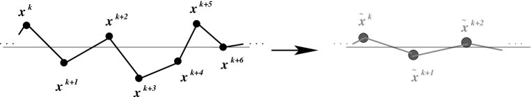
Figure 4: A quasi-linear brane-chain. The dots are locations of D-branes in transverse space, labelled before and after blocking up by $x^{k}$ and ${\tilde{x}}^{k}$ respectively (the worldvolume coordinates have been suppressed).

where ${\vec{x}}_{k}=(x_{k}^{1},x_{k}^{2},\ldots)\$ is the vector representing the location of the $k$-th D-brane in the transverse space. However, there are hoards of gauge transformations that correspond to this same brane-chain in physical space. A gauge-invariant way to block up would be to perform a weighted blocking up of each set of matrices in a given gauge orbit. A schematic example of such a weight is $\Pi_{i,j}\ e^{-|{\vec{x}}_{i}-{\vec{x}}_{j}|^{2}}$. This ensures that gauge equivalent configurations with large differences in the eigenvalues $x_{i}$ are suppressed while matrices whose eigenvalue entries are near each other dominate, while still retaining manifest gauge invariance.
In general, mapping a general spatial lattice-like structure to an ordering of D-brane matrix eigenvalues that is faithful physically under blocking up appears contrived. Indeed such mappings are perhaps only possible in some regions of moduli space. It would be interesting to study specific brane configurations, quivers and deconstructions to examine whether blocking up branes gives any new insights into the commutative case.

Appendix B Other ways to block up branes

It is important to note that one can cook up other ways to block up D-branes. For example, consider blocking up as

$$X^{i} = {\rm diag}\biggl{(}x^{i}_{1},x^{i}_{2},x^{i}_{3},x^{i}_{4},x^{i}_{5},x^{i}_{6},\ldots\biggr{)}\ \rightarrow\ {\tilde{X}}^{i}={\rm diag}\biggl{(}{x^{i}_{1}+x^{i}_{2}\over 2}{\bf 1_{2}},{x^{i}_{3}+x^{i}_{4}\over 2}{\bf 1_{2}},{x^{i}_{5}+x^{i}_{6}\over 2}{\bf 1_{2}},\ldots\biggr{)}$$ (141)

$$\ \rightarrow\ {\tilde{\tilde{X}}}^{i}={\rm diag}\biggl{(}{x^{i}_{1}+x^{i}_{2}+x^{i}_{3}+x^{i}_{4}\over 2}{\bf 1_{4}},{x^{i}_{5}+x^{i}_{6}+x^{i}_{7}+x^{i}_{8}\over 2}{\bf 1_{4}},\ldots\biggr{)}\ \rightarrow\ \ldots$$

This clearly does not reduce the rank of the gauge group even for finite $N$. What we have done is to in fact enhance gauge symmetry, from a $U(k)\times U(k)$ in each block to a $U(2k)$. Indeed the limit of this kind of blocking up for $N$ branes is a $U(N)$ gauge theory. Thus we have integrated $in$ the massive open string modes that were stretched between noncoincident branes within a block. This kind of blocking up therefore moves towards the ultraviolet of the field theory, as opposed to the infrared as before.
Indeed, consider the supergravity solution dual to this (${\cal N}{=}4$) field theory configuration on the Coulomb branch – this is a multicenter D3-brane supergravity solution [28]. Then the centers in the corresponding block go from two separated $N$ brane centers to a single $2N$ brane center. Physically what this means is that we have approximated a multicenter background by an averaged single center background with the same mass – to leading order, one does not resolve the separation between the centers. Thus this is blocking up in $spacetime$, while the previously discussed blocking up is in field theory space.

The basic point we are trying to make here is that since D-branes admit two dual descriptions, via gauge theory and via gravity, we can can approximate D-brane systems by blocking them up in two manifestly different ways. What we have illustrated in the bulk of this work is blocking up in field theory. This section gives a brief glimpse of what blocking up in spacetime is like, as an approximation scheme. Perhaps there are yet other physically relevant ways to block up branes with new physics.

References

-
[1]
See e.g.,
C. V. Johnson,
“D-brane Primer”, [hep-th/0007170] (on http://arxiv.org/);
W. Taylor, “Lectures on D-branes, gauge theories and M(atrices)”, [hep-th/9801182],
“M(atrix) theory : Matrix Quantum mechanics as a fundamental theory”, Rev. Mod. Phys. 73, 419 (2001), [hep-th/0101126];
M. R. Douglas, N. Nekrasov, “Noncommutative field theory”, Rev. Mod. Phys. 73, 977 (2001), [hep-th/0106048];
J. Harvey, “Komaba lectures on noncommutative solitons and D-branes”, [hep-th/0102076];
R. Szabo, “Quantum field theory on noncommutative spaces”, [hep-th/0109162]. - [2] E. Witten, “Bound states of strings and p-branes”, Nucl. Phys. B460, 335 (1996), [hep-th/9510135].
- [3] T. Banks, N. Seiberg, S. Shenker, “Branes from Matrices”, Nucl. Phys. B490, 91 (1997), [hep-th/9612157].
- [4] T. Banks, W. Fischler, S. Shenker, L. Susskind, “M-theory as a Matrix model : a conjecture”, Phys. Rev. D55, 5112 (1997), [hep-th/9610043].
- [5] N. Ishibashi, H. Kawai, Y. Kitazawa, A. Tsuchiya, “A large N reduced model as superstring”, Nucl. Phys. B498, 467 (1997), [hep-th/9612115].
- [6] R. C. Myers, “Dielectric branes”, JHEP 9912, 022 (1999), [hep-th/9910053]; see also R. C. Myers, “Non-abelian D-branes and noncommutative geometry”, Int. J. Mod. Phys. A16, 956 (2001), [hep-th/0106178].
- [7] E. Witten, “Noncommutative geometry and string field theory”, Nucl. Phys. B268, 253 (1986).
- [8] A. Connes, M. Douglas, A. Schwarz, “Noncommutative geometry and Matrix theory : Compactification on tori”, JHEP 9802, 003 (1998), [hep-th/9711162].
- [9] V. Schomerus, “D-branes and deformation quantization”, JHEP 9906, 030 (1999), [hep-th/9903205].
- [10] N. Seiberg, E. Witten, “String theory and noncommutative geometry”, JHEP 9909, 032 (1999), [hep-th/9908142].
- [11] D. Berenstein, V. Jejjala, R. Leigh, “Marginal and relevant deformations of field theories and noncommutative moduli spaces of vacua”, JHEP 0005 (2000), [hep-th/0005087].
- [12] See, e.g., the review, O. Aharony, S. .Gubser, J. Maldacena, H. Ooguri, Y. Oz, “Large N field theories, string theory and gravity”, Phys. Rept. 323, 183 (2000), [hep-th/9905111].
- [13] See, e.g., L. Rastelli, A. Sen, B. Zwiebach, “Vacuum string field theory”, [hep-th/0106010], and references therein.
-
[14]
Besides various textbooks, the following papers/reviews give a good
description of block spins, Kadanoff scaling and critical phenomena :
K. G. Wilson, “Renormalization group and critical phenomena 1 : renormalization group and the Kadanoff scaling picture”, Phys. Rev. B4 3174 (1971);
“Renormalization group and critical phenomena 2 : Phase space cell analysis of critical behaviour”, Phys. Rev. B4 3184 (1971);
“The renormalization group : critical phenomena and the Kondo problem”, Rev. Mod. Phys. 47 773 (1975);
“The renormalization group and block spins”, Cornell U. preprint CLNS-319, Oct 1975;
K. G. Wilson, J. Kogut, “The renormalization group and the -expansion”, Phys. Rep. 12 75 (1974);
S. Shenker, Les Houches 1982 lectures on field theory and phase transitions;
J. Kogut, “Introduction to lattice gauge theory and spin systems”, Rev. Mod. Phys. 51, 659 (1979). - [15] A. Alekseev, A. Recknagel, V. Schomerus, “Noncommutative worldvolume geometries : branes on and fuzzy spheres”, JHEP 9909, 023 (1999), [hep-th/9908040], “Brane dynamics in background fluxes and noncommutative geometry”, JHEP 0005, 010 (2000), [hep-th/0003187].
- [16] N. Arkani-Hamed, A. Cohen, H. Georgi, “(De)constructing dimensions”, Phys. Rev. Lett. 86 4757 (2001), [hep-th/0104005]; C. Hill, S. Pokorski, J. Wang, “Gauge-invariant effective lagrangian for Kaluza-Klein modes”, Phys. Rev. D64, 105005 (2001), [hep-th/0104035].
- [17] N. Seiberg, “A note on background independence in noncommutative gauge theories, matrix model and tachyon condensation”, JHEP 0009, 003 (2000), [hep-th/0008013].
- [18] S. Minwalla, M. van Raamsdonk, N. Seiberg, “Noncommutative perturbative dynamics”, JHEP 0002, 020 (2000), [hep-th/9912072]; see also M. van Raamsdonk, “The meaning of infrared singularities in noncommutative gauge theories”, JHEP 0111, 006 (2001), [hep-th/0110093].
- [19] A. Matusis, L. Susskind, N. Toumbas, “The IR/UV connection in noncommutative gauge theories”, JHEP 0012, 002 (2000), [hep-th/0002075].
- [20] D. Gross, A. Hashimoto, N. Itzhaki, “Observables of noncommutative gauge theories”, Adv. Theor. Math. Phys. 4, 893 (2000), [hep-th/0008075].
- [21] V. Sahakian, “Transcribing space-time data into matrices”, JHEP 0106 037 (2001), [hep-th/0010237].
- [22] S. Shenker, “Another length scale in string theory ?”, [hep-th/9509132].
- [23] M. Douglas, D. Kabat, P. Pouliot, S. Shenker, “D-branes and short distances in string theory”, Nucl. Phys. B485, 85 (1997), [hep-th/9608024].
- [24] D. Kabat, W. Taylor, “Spherical membranes in Matrix theory”, Adv. Theor. Math. Phys. 2, 181 (1998), [hep-th/9711078].
- [25] L. Cornalba, R. Schiappa, “Nonassociative star product deformations for D-brane worldvolumes in curved backgrounds”, Comm. Math. Phys. 225 33 (2002), [hep-th/0101219];
- [26] L. Alvarez-Gaume, D. Freedman, S. Mukhi, “The background field method and the ultraviolet structure of the supersymmetric nonlinear sigma model”, Annals. Phys. 134, 85 (1981) ; S. Mukhi, “The geometric background field method, renormalization and the Wess-Zumino term in nonlinear sigma models”, Nucl. Phys. B264, 640 (1986).
- [27] N. Arkani-Hamed, A. Cohen, H. Georgi, “Twisted supersymmetry and the topology of theory space”, JHEP 0207, 020 (2002), [hep-th/0109082].
- [28] P. Kraus, F. Larsen, S. Trivedi, “The Coulomb branch of gauge theories from rotating branes”, JHEP 9903 003 (1999), [hep-th/9811120]; see also I. Klebanov, E. Witten, “AdS/CFT correspondence and symmetry breaking”, Nucl. Phys. B556, 89 (1999), [hep-th/9905104].
- [29] S. Vaidya, “Perturbative dynamics on the fuzzy and ”, Phys. Lett. B512, 403 (2001), [hep-th/0102212].
- [30] E. Brezin, J. Zinn-Justin, “Renormalization group approach to matrix models”, Phys. Lett. B288, 54 (1992), [hep-th/9206035].
- [31] K. Narayan, M. Ronen Plesser, “Coarse-graining quivers”, [hep-th/0309171].