Quantum Gravitational Corrections to the Nonrelativistic Scattering Potential of Two Masses

Abstract

We treat general relativity as an effective field theory, obtaining the full nonanalytic component of the scattering matrix potential to one-loop order. The lowest order vertex rules for the resulting effective field theory are presented and the one-loop diagrams which yield the leading nonrelativistic post-Newtonian and quantum corrections to the gravitational scattering amplitude to second order in $G$ are calculated in detail. The Fourier transformed amplitudes yield a nonrelativistic potential and our result is discussed in relation to previous calculations. The definition of a potential is discussed as well and we show how the ambiguity of the potential under coordinate changes is resolved.

1 Introduction

The idea that a field theory need not be strictly renormalizable in the traditional sense yet can still yield useful quantum predictions when treated as an effective field theory [1] has been clearly demonstrated in chiral perturbation theory and in other applications[2]. Quantum loop calculations lead to well defined results in the low energy limit. Interestingly, such methods can also be applied to general relativity. As an effective field theory, the quantization of general relativity can be carried out in a consistent way, since the troublesome singularities which occur for various types of matter sources in traditional renormalization schemes [3, 4, 5, 6, 7] can be absorbed into phenomenological constants which characterize the effective action of the theory. This effective field theory approach offers then a possible way around the familiar renormalization difficulties of general relativity in the low energy regime and, using this approach with background field quantization [8] of general relativity, one of us [9, 10] some years ago derived the leading quantum and classical corrections to the Newtonian potential of two large non-relativistic masses. This calculation has since been the focus of a number of publications [11, 12, 13, 14], and this work continues, most recently in the paper [15]. Unfortunately, due to difficulty of the calculation and its myriad of tensor indices there has been little agreement among these various authors. The classical component of the correction has previously been discussed in the papers by[16, 17, 18, 19, 20], and here there is general agreement although, as we shall discuss, there exists an unavoidable ambiguity in defining the potential. The basic disagreements lie rather in the quantum corrections and in the present paper we shall present what we believe to be the definitive result for the leading classical and quantum corrections of order $G^{2}$, using the full scattering amplitude as the definition of the non-relativistic potential.

We note that, as a prelude to this effort, in a recent paper [24] two of us have dealt with the the quantum and classical corrections to the Reissner-Nordström and Kerr-Newman metrics of charged scalars and fermions. Such quantum and classical corrections have also been considered from the viewpoint of a scattering potential in a paper [25] by one of us. Recently we have also calculated the full classical and quantum corrections to the Schwarzshild and Kerr metrics of scalars and fermions [26] and have shown in detail how the higher order gravitational contributions to these metrics emerge from loop calculations. In the present paper then we consider the corresponding calculation of the full scattering amplitude.

Of course, treating general relativity as an effective field theory is carried out at the cost of introducing a never ending set of additional higher derivative couplings into the theory. In this sense Einstein’s general relativity is still a perfectly valid theory for gravitational interactions—although now it represents only the the minimal theory. At some stage additional derivative couplings must be appended to the Einstein action, signifying manifestations of the higher energy component of the effective field theory. However, the low energy scattering potential is free from these new couplings and represents a model-independent result for quantum gravity.

This calculation is possible because the post-Newtonian and quantum corrections which we consider are determined fully by the non-analytic pieces of the one loop amplitude generated by the lowest order Einstein action. Of course, in order to deal with the ultraviolet divergences which arise at one loop, one must renormalize the parameters of higher derivative terms in the action. However, such pieces will only affect the analytic parts of the one-loop amplitude, and will not contribute to our potential.

We will employ the same conventions as in our previous papers, namely ($\hbar=c=1$) as well as the Minkowski metric convention $(+1,-1,-1,-1)$. We will begin in section 2 with a very short introduction to the effective field theory quantization of general relativity and focus here especially on the distinction between non-analytic and analytic contributions to the scattering amplitude. We also include a discussion of the definition of the non-relativistic potential.

Next in section 3 we evaluate the diagrams which contribute to the scattering and examine in detail the results for the various components. The resulting nonanalytic piece of the scattering amplitude is then used in order to construct the leading corrections to the nonrelativistic gravitational potential. We also discuss our result in relation to previous calculations and attempt to sort out the various inconsistencies in the published numbers. Finally in a concluding section we summarize our findings.

2 Review of general relativity as an effective field theory

We begin with a brief review of general relativity, the Lagrangian of which (not including a cosmological term) is

$${\cal L}=\sqrt{-g}\left[\frac{2R}{\kappa^{2}}+{\cal L}_{\text{matter}}\right]$$ (1)

where $\kappa^{2}=32\pi G$ is the gravitational coupling, $R^{\mu}_{\ \nu\alpha\beta}\equiv\partial_{\alpha}\Gamma_{\nu\beta}^{\mu}-\partial_{\beta}\Gamma_{\nu\alpha}^{\mu}+\Gamma^{\mu}_{\sigma\alpha}\Gamma_{\nu\beta}^{\sigma}-\Gamma_{\sigma\beta}^{\mu}\Gamma_{\nu\alpha}^{\sigma}$ is the curvature tensor, and $g$ denotes the determinant of the metric field $g_{\mu\nu}$. Here $\sqrt{-g}{\cal L}_{\rm matter}$ is a covariant Lagrangian for the matter fields, and in principle any type of matter field could be included. This action defines the classical theory of general relativity.

In order to treat Eq. 1 as an effective field theory one must include all possible higher derivative couplings of the fields in the gravitational Lagrangian. In this way any field singularities generated by loop diagrams can be associated with some component of the action and hence can be absorbed via a simple redefinition of the coupling constants of the theory. Treating all such coupling coefficients as experimentally determined quantities, the effective field theory is then finite and contains no singularities at any finite order of the loop expansion.

We can consequently write an effective action for pure general relativity as

$${\cal L}=\sqrt{-g}\left\{\frac{2R}{\kappa^{2}}+c_{1}R^{2}+c_{2}R^{\mu\nu}R_{\mu\nu}+\ldots\right\}$$ (2)

where the ellipses denote that the effective action is in fact an infinite series—at each new loop order additional higher derivative terms must be taken into account. This Lagrangian includes all possible higher derivative couplings, and every coupling constant in the Lagrangian is considered to be determined empirically. Similarly one must include higher derivative contributions to the matter Lagrangian in order to treat this piece of the Lagrangian as an effective field theory. Details of such considerations can be found in the papers [9, 10].

In our calculations we will consider only the non-analytic contributions, which are generated by the propagation of two or more massless particles in the Feynman diagrams. Such nonanalytic effects are long-ranged and, in the low energy limit of the effective field theory, they dominate over the analytic contributions which arise from the propagation of massive modes. The typical non-analytic terms we will consider are of the type: $1/\sqrt{-q^{2}}$ and $\ln q^{2}$—while the typical analytic contribution is a power series in $q$. The feature that the analytic contributions originate from the propagation of massive particles while the non-analytic effect comes from massless propagation can be seen directly by Taylor expanding the two types of propagators. Indeed the massless propagator $1/q^{2}$ cannot be expanded in a series, while we have the obvious representation for the massive propagator: $1/(q^{2}-m^{2})=-1/m^{2}(1-q^{2}/m^{2}+\ldots)$. Thus the massive parts of the diagrams will always be expandable and hence analytic—while the massless contributions have the possibility of generating nonanalytic components. It should be noted that such nonanalytic pieces of the scattering amplitude are essential to the unitarity of the S-matrix.

2.1 Definition of the potential

Before proceeding to the actual calculations, it is important to note that the precise definition of a potential in a relativistic quantum field theory such as general relativity is not obvious. In the original papers, the one-particle-irreducible potential was calculated [9, 10]. However, additional diagrams are required in order to relate this quantity to physical observables. Subsequent work has considered alternative definitions. Clearly a gravitational potential should be gauge invariant in order to make physical sense, but one can choose between various definitions of the potential depending on the physical situation, how the total energy is defined, etc. In QCD one can always turn to the venerable Wilson loop description but there exists no standard Wilson loop description for the gravitational potential, although some work has been done in this direction [21] using the Arnowitt-Deser-Misner formula for the total energy of the gravitational system. Such an approach to the gravitational potential has been taken in the paper [11]. For yet another approach to the Newtonian potential, see [22]. An alternative path is to use the scattering amplitude itself to define the potential. This description of the potential seems to us the simplest and most intuitive picture and has been employed by a number of authors [17, 18, 16, 12, 23, 15]. Herein then we shall also use the full scattering amplitude in order to represent the potential, defining

$$\langle f|T|i\rangle \equiv (2\pi)^{4}\delta^{(4)}(p-p^{\prime})({\cal M}(q))$$ (3)

$$= -(2\pi)\delta(E-E^{\prime})\langle f|\tilde{V}({\bf q})|i\rangle$$

where $p,p^{\prime}$ is the incoming, outgoing four-momentum. The corresponding coordinate space representation can be found by taking the nonrelativistic limit and Fourier-transforming, yielding the result

$$V({\bf x})=\frac{1}{2m_{1}}\frac{1}{2m_{2}}\int\frac{d^{3}q}{(2\pi)^{3}}e^{i{\bf q}\cdot{\bf x}}{\cal M}(\vec{q})$$ (4)

and will serve as our definition of the nonrelativistic potential.

It should be noted, however, that this is not the only way in which to define the potential $V({\bf q})$ in terms of the scattering amplitude. One could, for example, subtract off the second order Born contributions, which would lead to the nonrelativistic potential used in bound state quantum mechanics and would be equivalent to using the prescription

$$i\langle f|T|i\rangle = -2\pi i\delta(E-E^{\prime})$$ (5)

$$\times \bigg{[}\langle f|\tilde{V}_{bs}({\bf q})|i\rangle+\sum_{n}\frac{\langle f|\tilde{V}_{bs}({\bf q})|n\rangle\langle n|\tilde{V}_{bs}({\bf q})|i\rangle}{E-E_{n}+i\epsilon}+\ldots\bigg{]}$$

The definition of the bound state potential is discussed in detail in  [17]. In particular, in a Hamiltonian treatment there are also terms in the Hamiltonian involving $Gp^{2}/r$ that contribute at the same order. The relation of the bound state potential $\tilde{V}_{bs}({\bf q})$, in Einstein-Infeld-Hoffmann coordinates, to the lowest order scattering potential is

$$\tilde{V}_{bs}(r)=V(r)+{7Gm_{1}m_{2}(m_{1}+m_{2})\over 2c^{2}r^{2}}$$ (6)

2.2 The diagrams contributing to the nonanalytic component of the scattering matrix

We will consider here only the nonanalytic contributions from the one-loop diagrams. Since many diagrams yield purely analytic contributions to the S-matrix, such diagrams need not be considered and will be omitted from the beginning. The diagrams which do yield nonanalytic contributions to the $S$ matrix amplitude are those containing two or more massless propagating particles. A typical such amplitude will be of the form

$${\cal M}\sim\Big{(}A+Bq^{2}+\ldots+\alpha\kappa^{4}\frac{1}{q^{2}}+\beta_{1}\kappa^{4}\ln(-q^{2})+\beta_{2}\kappa^{4}\frac{m}{\sqrt{-q^{2}}}+\ldots\Big{)}$$ (7)

Here the coefficients $A,B,\ldots$ correspond to analytic pieces which are of no interest to us, as these terms will only dominate in the high energy regime of the effective theory. Rather, the $\alpha,\beta_{1},\beta_{2},\ldots$ coefficients correspond to the nonlocal, nonanalytic contributions to the amplitude and are the ones which we seek. In particular, the $\beta_{1},\beta_{2}$ terms will yield the leading post-Newtonian and quantum corrections to the potential.

3 Results for the Feynman diagrams

In this section we will present our results. All diagrams have been performed both by hand and by computer. In order to evaluate the diagrams by computer, an algorithm for Maple 7 (TM) was developed. This program contracts the various indices and perform the loop integrations. All results obtained this way were confirmed results obtained by hand. The resulting amplitudes were then Fourier transformed to produce the scattering potential, and only the nonanalytic pieces of the amplitude were retained. For this part of the calculation, the following Fourier integrals are useful:

$$\begin{split}\int\frac{d^{3}q}{(2\pi)^{3}}~{}e^{i{\bf q}\cdot{\bf r}}\frac{1}{|{\bf q}|^{2}}&=\frac{1}{4\pi r}\\ \int\frac{d^{3}q}{(2\pi)^{3}}~{}e^{i{\bf q}\cdot{\bf r}}\frac{1}{|{\bf q}|}&=\frac{1}{2\pi^{2}r^{2}}\\ \int\frac{d^{3}q}{(2\pi)^{3}}~{}e^{i{\bf q}\cdot{\bf r}}\ln({\bf q}^{2})&=\frac{-1}{2\pi r^{3}}\\ \end{split}$$ (8)

After this brief introduction, we proceed to give the results for each diagram in turn. Note that the basic vertices needed for our calculation are given in Appendix A.

3.1 The tree diagram

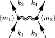
1(a)

Figure 1: The tree diagram giving Newtons law.

The result for this diagram in the nonrelativistic limit is the well-known lowest order tree-level result which yields the Newtonian potential. We define the diagram using the Feynman rules as:

$$iM_{1(a)}(\vec{q})=\tau^{\mu\nu}_{1}(k_{1},k_{2},m_{1})\Big{[}\frac{i{\cal P}_{\mu\nu\alpha\beta}}{q^{2}}\Big{]}\tau_{1}^{\alpha\beta}(k_{3},k_{4},m_{2})$$ (9)

where $q=k_{1}-k_{2}=k_{4}-k_{3}$. Contracting all indices and taking the nonrelativistic limit, we find

$$M_{1(a)}(\vec{q})=-{4\pi Gm_{1}m_{2}\over\vec{q}^{2}}$$ (10)

whose Fourier transform produces the scattering potential

$$V_{1(a)}(r)=-\frac{G{m_{1}}{m_{2}}}{r}$$ (11)

which is indeed the familiar Newtonian form.

3.2 The box and crossed box diagrams

2(a)

2(b)

Figure 2: The box and crossed box diagrams which contribute to the non-analytic component of the potential.

We can write the contributions of these two diagrams as

$$M_{2a} =\int\frac{d^{4}l}{(2\pi)^{4}}\tau_{1}^{\mu\nu}(k_{1},k_{1}+l,m_{1})\tau_{1}^{\rho\sigma}(k_{1}+l,k_{2},m_{1})$$ (12)

$$\times\tau_{1}^{\alpha\beta}(k_{3},k_{3}-l,m_{2})\tau_{1}^{\gamma\delta}(k_{3}-l,k_{4},m_{2})$$

$$\times\Big{[}\frac{i}{(k_{1}+l)^{2}-m_{1}^{2}}\Big{]}\Big{[}\frac{i}{(k_{3}-l)^{2}-m_{2}^{2}}\Big{]}\Big{[}\frac{i{\cal P}_{\mu\nu\alpha\beta}}{l^{2}}\Big{]}\Big{[}\frac{i{\cal P}_{\rho\sigma\gamma\delta}}{(l+q)^{2}}\Big{]}$$

for the box and

$$M_{2b} =\int\frac{d^{4}l}{(2\pi)^{4}}\tau_{1}^{\mu\nu}(k_{1},k_{1}+l,m_{1})\tau_{1}^{\rho\sigma}(k_{1}+l,k_{2},m_{1})$$ (13)

$$\times\tau_{1}^{\gamma\delta}(k_{3},l+k_{4},m_{2})\tau_{1}^{\alpha\beta}(l+k_{4},k_{4},m_{2})$$

$$\times\Big{[}\frac{i}{(k_{1}+l)^{2}-m_{1}^{2}}\Big{]}\cdot\Big{[}\frac{i}{(l+k_{4})^{2}-m_{2}^{2}}\Big{]}\cdot\Big{[}\frac{i{\cal P}_{\mu\nu\alpha\beta}}{l^{2}}\Big{]}\Big{[}\frac{i{\cal P}_{\rho\sigma\gamma\delta}}{(l+q)^{2}}\Big{]}$$

for the cross box. These diagrams are among the most challenging that we will encounter, due to the rather complicated integrals—containing four propagators—which must be evaluated. However, those pieces of the amplitude which are loop momentum-dependent simplify, due to the feature that the external particles are on shell and by the fact that we are only seeking the nonanalytic pieces of the scattering amplitude. This allows reduction of parts of the amplitude initially having four propagators to pieces where effectively only three or two propagators remain. An example of this simplification can be seen by the replacement of the integral

$$\int \frac{d^{4}l}{(2\pi)^{2}}\frac{l\cdot k_{1}}{l^{2}(l+q)^{2}((l+k_{1})^{2}-m_{1}^{2})((l-k_{3})^{2}-m_{2}^{2})}$$ (14)

$$=\frac{1}{2}\int\frac{d^{4}l}{(2\pi)^{2}}\frac{((l+k_{1})^{2})-l^{2}-m_{1}^{2}}{l^{2}(l+q)^{2}((l+k_{1})^{2}-m_{1}^{2})((l-k_{3})^{2}-m_{2}^{2})}$$

by

$$\frac{1}{2}\int\frac{d^{4}l}{(2\pi)^{2}}\frac{1}{l^{2}(l+q)^{2}((l-k_{3})^{2}-m_{2}^{2})}$$ (15)

because the $l^{2}$ part will not contribute to the nonanalytic component. The integrals with three or two propagator terms are explicitly given in Appendix B. Another simplification arises when the momentum $q^{\mu}$ contracts with a loop momentum $l^{\mu}$ in the numerator. An example is

$$\int \frac{d^{4}l}{(2\pi)^{2}}\frac{l\cdot q}{l^{2}(l+q)^{2}((l+k_{1})^{2}-m_{1}^{2})((l-k_{3})^{2}-m_{2}^{2})}$$ (16)

$$=\frac{1}{2}\int\frac{d^{4}l}{(2\pi)^{2}}\frac{((l+q)^{2})-l^{2}-q_{1}^{2}}{l^{2}(l+q)^{2}((l+k_{1})^{2}-m_{1}^{2})((l-k_{3})^{2}-m_{2}^{2})}$$

which simplifies to

$$-\frac{1}{2}\int\frac{d^{4}l}{(2\pi)^{2}}\frac{q^{2}}{l^{2}(l+q)^{2}((l-k_{3})^{2}-m_{2}^{2})}$$ (17)

Via these simplifications one can reduce the box and cross box amplitudes to a reduced piece consisting only of integrals with two or three propagators and a component with the basic form of the box and crossed box integrals, i.e., with no loop momentum terms in the numerator. Then, using the integrals presented in Appendix B, performing the above-described contractions in the two diagrams, and taking the nonrelativistic limit we end up with the result

$$M_{2(a)+2(b)}^{\rm red}(\vec{q})={46\over 3}G^{2}m_{1}m_{2}\log\vec{q}^{2}$$ (18)

for the momentum-reduced component of the box plus cross box and

$$M_{2(a)+2(b)}^{\rm irred}(\vec{q})=16G^{2}m_{1}m_{2}\log\vec{q}^{2}$$ (19)

for the irreducible piece. Fourier transforming, we find then the scattering potential contributions

$$V_{2(a)+2(b)}^{\rm red}(r)=-\frac{23}{3}\frac{m_{1}m_{2}G^{2}}{\pi r^{3}}$$ (20)

for the reducible component and

$$V_{2(a)+2(b)}^{\rm irred}(r)=-8\frac{m_{1}m_{2}G^{2}}{\pi r^{3}}$$ (21)

for the irreducible piece so that the total result for the box and cross box contribution to the potential is

$$V_{2(a)+2(b)}^{\rm tot}(r)=-\frac{47}{3}\frac{m_{1}m_{2}G^{2}}{\pi r^{3}}$$ (22)

These results are in agreement with those of  [15].

3.3 The triangle diagrams

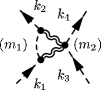
3(a)

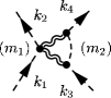
3(b)

Figure 3: The set of triangule diagrams contributing to the scattering potential.

The next pieces we will consider are the set of triangle diagrams, for which we find

$$M_{3(a)}(q) =\int{d^{4}l\over(2\pi)^{4}}\tau_{1}^{\mu\nu}(k_{1},l+k_{1},m_{1})\tau_{1}^{\alpha\beta}(l+k_{1},k_{2},m_{1})\tau_{2}^{\sigma\rho\gamma\delta}(k_{3},k_{4},m_{2})$$ (23)

$$\times\Big{[}\frac{i{\cal P}_{\alpha\beta\gamma\delta}}{(l+q)^{2}}\Big{]}\Big{[}\frac{i{\cal P}_{\mu\nu\sigma\rho}}{l^{2}}\Big{]}\Big{[}\frac{i}{(l+k_{1})^{2}-m_{1}^{2}}\Big{]}$$

and

$$M_{3(b)}(q) =\int{d^{4}l\over(2\pi)^{4}}\tau_{1}^{\sigma\rho}(k_{3},k_{3}-l,m_{2})\tau_{1}^{\gamma\delta}(k_{3}-l,k_{4},m_{2})\tau_{2}^{\mu\nu\alpha\beta}(k_{1},k_{2},m_{1})$$ (24)

$$\times\Big{[}\frac{i{\cal P}_{\mu\nu\sigma\rho}}{l^{2}}\Big{]}\Big{[}\frac{i{\cal P}_{\alpha\beta\gamma\delta}}{(l+q)^{2}}\Big{]}\Big{[}\frac{i}{(l-k_{3})^{2}-m_{2}^{2}}\Big{]}$$

The calculation of such diagrams yields no real complications— the integrals needed are quite straightforward and are presented in Appendix B. However, a significant simplification results from the use of the identity

$${\cal P}_{\gamma\delta\sigma\rho}{\cal P}_{\alpha\beta\mu\nu}\tau^{\sigma\rho\mu\nu}(k_{1},k_{2},m_{1})=\tau_{\gamma\delta\alpha\beta}(k_{1},k_{2},m_{1})$$ (25)

and, taking the nonrelativistic limit, we find for these two pieces

$$M_{3(a)}(\vec{q}) = -8G^{2}m_{1}m_{2}\left({7\over 2}\log\vec{q}^{2}+{\pi^{2}m_{1}\over|\vec{q}|}\right)$$

$$M_{3(b)}(\vec{q}) = -8G^{2}m_{1}m_{2}\left({7\over 2}\log\vec{q}^{2}+{\pi^{2}m_{2}\over|\vec{q}|}\right)$$ (26)

Our results for these diagrams agree with those of  [15], and the Fourier transformed result is

$$V_{3(a)+3(b)}(r)=-4\frac{G^{2}m_{1}m_{2}(m_{1}+m_{2})}{r^{2}}+28\frac{m_{1}m_{2}G^{2}}{\pi r^{3}}$$ (27)

3.4 The double-seagull diagram

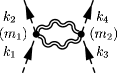
4(a)

Figure 4: The double-seagull diagram contribution to the scattering potential.

We have for the double-seagull term

$$M_{4(a)}(q) ={1\over 2!}\int{d^{4}l\over(2\pi)^{4}}\tau_{2}^{\alpha\beta\gamma\delta}(k_{1},k_{2},m_{1})\tau_{2}^{\sigma\rho\mu\nu}(k_{3},k_{4},m_{2})\times\Big{[}\frac{i{\cal P}_{\alpha\beta\mu\nu}}{(l+q)^{2}}\Big{]}\Big{[}\frac{i{\cal P}_{\gamma\delta\sigma\rho}}{l^{2}}\Big{]}$$ (28)

The double-seagull loop diagram is quite straightforward, and is simplified by use of the identity Eq. 25. Note, however, that there exists a symmetry factor of $1/2!$. The resulting amplitude is found to be

$$M_{4(a)}(\vec{q})=44G^{2}m_{1}m_{2}\log\vec{q}^{2}$$ (29)

whose Fourier transform yields the double-seagull contribution to the potential

$$V_{4(a)}(r)=-22\frac{m_{1}m_{2}G^{2}}{\pi r^{3}}$$ (30)

3.5 The vertex correction diagrams

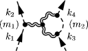
5(a)

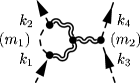
5(b)

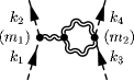
5(c)

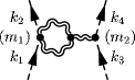
5(d)

Figure 5: The class of the graviton vertex corrections which yield nonanalytic corrections to the potential.

There exist two classes of vertex correction diagrams: For the massive loop diagrams, shown in Figures 5(a) and 5(b) we have

$$M_{5(a)}(q) ={d^{4}l\over(2\pi)^{4}}\tau_{1}^{\alpha\beta}(k_{1},k_{2},m_{1})\tau_{1}^{\mu\nu}(k_{3},k_{3}-l,m_{2})\tau_{1}^{\rho\sigma}(k_{3}-l,k_{4},m_{2})\tau_{3}^{\lambda\kappa\phi\epsilon(\gamma\delta)}(l,-q)$$ (31)

$$\times\Big{[}\frac{i{\cal P}_{\lambda\kappa\mu\nu}}{l^{2}}\Big{]}\Big{[}\frac{i{\cal P}_{\phi\epsilon\rho\sigma}}{(l+q)^{2}}\Big{]}\Big{[}\frac{i{\cal P}_{\alpha\beta\gamma\delta}}{q^{2}}\Big{]}\Big{[}\frac{i}{(l-k_{3})^{2}-m_{2}^{2}}\Big{]}$$

and

$$M_{5(b)}(q) =\int{d^{4}l\over(2\pi)^{4}}\tau_{1}^{\alpha\beta}(k_{1},l+k_{1},m_{1})\tau_{1}^{\mu\nu}(l+k_{1},k_{2},m_{1})\tau_{1}^{\lambda\kappa}(k_{3},k_{4},m_{2})\tau_{3}^{\gamma\delta\rho\sigma(\phi\epsilon)}(-l,q)$$ (32)

$$\times\Big{[}\frac{i{\cal P}_{\alpha\beta\gamma\delta}}{l^{2}}\Big{]}\Big{[}\frac{i{\cal P}_{\mu\nu\rho\sigma}}{(l+q)^{2}}\Big{]}\Big{[}\frac{i{\cal P}_{\phi\epsilon\lambda\kappa}}{q^{2}}\Big{]}\Big{[}\frac{i}{(l+k_{1})^{2}-m_{1}^{2}}\Big{]}$$

while for the pure graviton loop diagrams shown in Figures 5(c) and 5(d)we have

$$M_{5(c)}(q) ={1\over 2!}\int{d^{4}l\over(2\pi)^{4}}\tau_{2}^{\lambda\kappa\epsilon\phi}(k_{3},k_{4},m_{2})\tau_{1}^{\alpha\beta}(k_{1},k_{2},m_{1})\tau_{3}^{\mu\nu\rho\sigma(\gamma\delta)}(l,-q)$$ (33)

$$\times\Big{[}\frac{i{\cal P}_{\mu\nu\lambda\kappa}}{l^{2}}\Big{]}\Big{[}\frac{i{\cal P}_{\rho\sigma\epsilon\phi}}{(l+q)^{2}}\Big{]}\Big{[}\frac{i{\cal P}_{\alpha\beta\gamma\delta}}{q^{2}}\Big{]}$$

and

$$M_{5(d)}(q) ={1\over 2!}\int{d^{4}l\over(2\pi)^{4}}\tau_{2}^{\rho\sigma\mu\nu}(k_{1},k_{2},m_{1})\tau_{1}^{\lambda\kappa}(k_{3},k_{4},m_{2})\tau_{3}^{\alpha\beta\gamma\delta(\epsilon\phi)}(-l,q)$$ (34)

$$\times\Big{[}\frac{i{\cal P}_{\mu\nu\gamma\delta}}{l^{2}}\Big{]}\Big{[}\frac{i{\cal P}_{\rho\sigma\alpha\beta}}{(l+q)^{2}}\Big{]}\Big{[}\frac{i{\cal P}_{\lambda\kappa\epsilon\phi}}{q^{2}}\Big{]}$$

The vertex correction diagrams are certainly the most challenging to perform, disregarding the box and crossed box diagrams, and the results go back to the original calculation of [9, 10]—however, due to an algebraic error, the original result quoted for the such diagrams was in error. Since that time, the results for the gravitational vertex corrections have been checked at length in various publications [13, 15]; however, until [26] the correct forms have not been given. Using the results of [26] and taking the nonrelativistic limit, we find the amplitudes,

$$M_{5(a)+5(b)}(\vec{q}) = 2G^{2}m_{1}m_{2}\left({\pi^{2}(m_{1}+m_{2})\over|\vec{q}|}+{5\over 3}\log\vec{q}^{2}\right)$$

$$M_{5(c)+5(d)}(\vec{q}) = -{52\over 3}G^{2}m_{1}m_{2}\log\vec{q}^{2}$$ (35)

whose Fourier transform yields the corrected results for the vertex modifications to the scattering potential:

$$V_{5(a)+5(b)}(r)=\frac{G^{2}m_{1}m_{2}(m_{1}+m_{2})}{r^{2}}-\frac{5}{3}\frac{m_{1}m_{2}G^{2}}{\pi r^{3}}$$ (36)

and

$$V_{5(c)+5(d)}(r)=\frac{26}{3}\frac{m_{1}m_{2}G^{2}}{\pi r^{3}}$$ (37)

where again we note the presence of a symmetry factor $1/2!$ in the case of the pure graviton loop diagram. Our results for these diagrams are not in agreement with previous calculations. For the vertex correction diagrams $5(a)$ and $5(b)$, there is total disagreement with our result. However, we have performed a very detailed analysis of the vertex diagrams in our companion paper [26], showing how the classical ingredients match in detail those required by the classical Schwartzschild metric. The quantum vertex result of [15] is the same as that of [13] and the latter yields an incorrect classical metric (Ref. [15] does not display their classical vertex correction). On the other hand, our detailed evaluation of the metric correction in [26] gives us confidence in the correctness of our result.

3.6 The vacuum polarization diagram

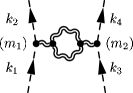
6(a)

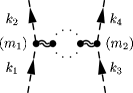
6(b)

Figure 6: The vacuum polarization diagrams which contribute to the potential. Note that there exists a ghost diagram along with the graviton loop.

The result for the vacuum polarization contribution can be found from the amplitude

$$M_{6(a)+6(b)}(q)=\tau_{\rho\sigma}(k_{1},k_{2},m_{1}){i{\cal P}^{\rho\sigma\lambda\xi}\over q^{2}}\Pi_{\lambda\xi\mu\nu}(q){i{\cal P}^{\mu\nu\gamma\delta}\over q^{2}}\tau_{\gamma\delta}(k_{3},k_{4},m_{2})$$ (38)

where the vacuum polarization tensor is found from the effective Lagrangian obtained by ’t Hooft and Veltman [3, 4, 5]—

$${\cal L}=-{1\over 16\pi^{2}}\log\vec{q^{2}}\left({1\over 120}R^{2}+{7\over 20}R_{\mu\nu}R^{\mu\nu}\right)$$ (39)

and is given by

$$\hat{\Pi}_{\alpha\beta,\gamma\delta} = -{2G\over\pi}\log(-q^{2})\left[{21\over 120}q^{4}I_{\alpha\beta,\gamma\delta}+{23\over 120}q^{4}\eta_{\alpha\beta}\eta_{\gamma\delta}\right.$$

$$- \left.{23\over 120}q^{2}(\eta_{\alpha\beta}q_{\gamma}q_{\delta}+\eta_{\gamma\delta}q_{\alpha}q_{\beta})\right.$$

$$- \left.{21\over 240}q^{2}(q_{\alpha}q_{\delta}\eta_{\beta\gamma}+q_{\beta}q_{\delta}\eta_{\alpha\gamma}+q_{\alpha}q_{\gamma}\eta_{\beta\delta}+q_{\beta}q_{\gamma}\eta_{\alpha\delta})+{11\over 30}q_{\alpha}q_{\beta}q_{\gamma}q_{\delta}\right]$$

(41)

Contracting the various indices, we find a result

$$M_{6(a)+6(b)}(\vec{q})={43\over 15}G^{2}m_{1}m_{2}\log\vec{q}^{2}$$ (42)

which is equivalent to that originally derived in [9, 10]. After Fourier transforming we find a contribution to the scattering potential

$$V_{6(a)+6(b)}(r)=-\frac{43}{30}\frac{m_{1}m_{2}G^{2}}{\pi r^{3}}$$ (43)

which is in agreement with that given by [15].

4 The result for the gravitational potential

Adding up all the corrections to the non-relativistic potential we have our final result

$$V(r)=-{Gm_{1}m_{2}\over r}\left[1+3\frac{G(m_{1}+m_{2})}{r}+\frac{41}{10\pi}\frac{G\hbar}{r^{2}}\right]$$ (44)

The classical term in this potential agrees with Eq. 2.5 of Iwasaki[17].

However, we note that the quantum component of the potential is not equivalent to any previous published result [9, 10, 11, 12, 13, 15]. As described above, we believe this result to be to definitive form of the nonrelativistic scattering matrix potential. Our results agree with [15] for all diagrams except the vertex corrections However we have multiple checks on the vertex correction, as we have seen that our version leads exactly to the required form of the classical Schwarzschild metric, for both fermions and bosons.

4.1 A Potential Ambiguity

There is an important issue concerning the potential that has not been thusfar much discussed in the literature—that both the classical and quantum corrections to the potential are in some sense ambiguous. For the classical correction, this realization goes back to the papers of [18, 19, 20], and these arguments generalize readily to the quantum component. In this section we discuss this ambiguity and argue that at one loop order our calculation of the quantum correction does have a well defined meaning.

As explored in [18] the classical post-Newtonian potential is not invariant under a coordinate transformation of the form

$$r\rightarrow r\Big{[}1+\alpha\frac{G(m_{1}+m_{2})}{r}\Big{]}~{}.$$ (45)

We are always free to make such a coordinate change, and that given in Eq. 45 modifies the classical correction to the potential via

$$\frac{Gm_{1}m_{2}}{r}\left[1+c\frac{G(m_{1}+m_{2})}{r}\right]\rightarrow\frac{Gm_{1}m_{2}}{r}\left[1+(c-\alpha)\frac{G(m_{1}+m_{2})}{r}\right]$$ (46)

Following [18, 20] the ambiguity can be seen to arise in a field theory calculation through a modification of the graviton propagator

$$\frac{1}{q^{2}}=\frac{1}{q_{0}^{2}-{\vec{q}}^{2}}$$ (47)

accomplished by using the energy conservation in the following identical way which holds true for general $x$.

$$\frac{1}{\frac{1}{2}(1-x)(({p_{2}}_{0}-{p_{1}}_{0})^{2}+({p_{4}}_{0}-{p_{3}}_{0})^{2}))-x({p_{2}}_{0}-{p_{1}}_{0})({p_{4}}_{0}-{p_{3}}_{0})-{\vec{q}}^{2}}$$ (48)

Using this propagator in order to derive the gravitational potential, the result will in general depend on $x$, with the relation to the coordinate change being $\alpha=-\frac{1}{4}(1-x)$. Not only will the terms of order $\frac{G^{2}}{r^{2}}$ depend on $x$, but so will the corrections of order $\Big{(}\frac{G}{r}\Big{)}\Big{(}\frac{v}{c}\Big{)}$. This indicates that the post-Newtonian part of the static gravitational potential is not well-defined in and of itself.

The coordinate ambiguity also generalizes to the quantum part of the potential. There exists a coordinate redefinition

$$r\to r\left[1+\beta{G\hbar\over r^{2}}\right]$$ (49)

which changes the coefficient of the quantum term in the potential

$$\frac{Gm_{1}m_{2}}{r}\left[1+d\frac{G\hbar}{r^{2}}\right]\rightarrow\frac{Gm_{1}m_{2}}{r}\left[1+(d-\beta)\frac{G\hbar}{r^{2}}\right]$$ (50)

Therefore, we need to address the uniqueness of the quantum correction to the potential.

Since general relativity is invariant under coordinate shifts, if the potentials are changed there must exist other modifications that compensate for these changes, leaving the resulting physics invariant. Within a Hamiltonian formulation, these modifications take the form of momentum-dependent pieces—in order to make the potential well defined, one must also specify the momentum terms in the Hamiltonian.

First we examine the classical ambiguity. Classically there are two dimensionless variables available for the expansion away from the Newtonian limit

$${p^{2}\over m^{2}}~{}~{},~{}~{}{Gm\over r}$$ (51)

In bound state problems these quantities appear at the same order, as can be seen by use of the virial theorem. In the Hamiltonian the leading terms are order

$$H_{1}\sim{p^{2}\over m},~{}~{}{Gm^{2}\over r}$$ (52)

and are unambiguous. At next order we have pieces of the form

$$H_{2}\sim{p^{4}\over m^{3}},~{}~{}{Gm^{2}\over r}{Gm\over r},~{}~{}({Gm\over r})({p^{2}\over m})$$ (53)

There exists an ambiguity between the last two of these terms arising from a coordinate change, but this effect cancels for physical observables, as shown explicitly in [18]. Writing the Hamiltonian in the center of mass frame to post-Newtonian order, we have

$$H = \left(\frac{{\bf p}^{2}}{2m_{1}}+\frac{{\bf p}^{2}}{2m_{2}}\right)-\left(\frac{{\bf p}^{4}}{8m_{1}^{3}}+\frac{{\bf p}^{4}}{8m_{2}^{3}}\right)$$ (54)

$$- \frac{Gm_{1}m_{2}}{r}\left[1+a\frac{\bf p^{2}}{m_{1}m_{2}}+b\frac{({\bf p\cdot\hat{r}})^{2}}{m_{1}m_{2}}+c{G(m_{1}+m_{2})\over r}\right]$$

In the standard Einstein-Infeld-Hoffmann coordinates, the coefficients $a,b,c$ have the values

$$a = \frac{1}{2}\left[1+3\frac{(m_{1}+m_{2})^{2}}{m_{1}m_{2}}\right]$$

$$b = {1\over 2}$$

$$c = -\frac{1}{2}$$ (55)

but under the coordinate transformation of Eq. 45, one finds the modifications

$$a \to \frac{1}{2}\left[1+(3+2\alpha)\frac{(m_{1}+m_{2})^{2}}{m_{1}m_{2}}\right]$$

$$b \to \frac{1}{2}-\alpha\frac{(m_{1}+m_{2})^{2}}{m_{1}m_{2}}$$

$$c \to -\frac{1}{2}-\alpha$$ (56)

Therefore, in order to specify the correction to the static potential, one needs also to identify the momentum coordinates. In particular, the classical potential calculated by Iwasaki is that appropriate for Einstein-Infeld-Hoffmann coordinates.

This classical ambiguity has not been worked out explicitly at the following order in the expansion, but the general pattern is apparent. Specifically, at the next order one has four types of terms

$$H_{3}\sim\frac{p^{6}}{m^{5}},~{}~{}\frac{p^{4}}{m^{3}}\left({Gm\over r}\right),~{}\frac{p^{2}}{m}\left({Gm\over r}\right)^{2},~{}~{}{Gm^{2}\over r}\left({Gm\over r}\right)^{2}.$$ (57)

The last term here is noteworthy because it goes like $1/r^{3}$—i.e. like the quantum correction in the potential—but it is distinguishable by its mass dependence plus the fact that it is order $G^{3}$. Such terms will also be ambiguous under a coordinate transformation, but the effects will cancel among the effects terms of this order. So the“classical” coordinate change above does change the $1/r^{3}$ term in the potential, but has a specific form and the effects cancels among other classical terms in the Hamiltonian.

Now let us examine the quantum effects, keeping only one power of the quantum expansion parameter

$${G\hbar\over r^{2}}$$ (58)

The quantum potential will enter the Hamiltonian at order

$$H_{q}={Gm^{2}\over r}{G\hbar\over r^{2}}$$ (59)

and the other term of this order is

$$H_{qp}\sim{p^{2}\over m}{G\hbar\over r^{2}}$$ (60)

If one makes the“quantum” coordinate change of Eq. 49 , this will generate such a term in the Hamiltonian, which for physical observables cancels the effect of the change in the potential. Therefore in order to make the quantum correction to the potential well defined, one must specify the value of the terms contained in $H_{qp}$. However, the important point is that, in any coordinates in which one calculates quantum corrections, one will not generate a term such as $H_{qp}$. This is because all quantum effects that involve the interparticle separation $r$ arise from loop diagrams of order $G^{2}$ while $H_{qp}$ has only a single power of $G$. Quantum effects on a single particle line are of order $G$ but do not involve $r$, while those involving two lines are of order $G^{2}$. Since all calculations yield no term of the form $H_{qp}$, they must give the same quantum potential. The fully specified quantum potential is that one in the coordinates where $H_{qp}$ vanishes. This, of course, is then the one that we have calculated. We conclude that, despite the expected general coordinate invariance, the calculated quantum potential is a well defined quantity to this order.

5 Discussion

The scattering amplitude has been used to provide a solid definition of the quantum corrections to the Newtonian potential. Our basic calculation is of certain nonanalytic terms in momentum space, the $\sqrt{-q^{2}}$ and $q^{2}\ln-q^{2}$ terms. A transformation of these terms to coordinate space allows us to interpret these as long distance corrections to the potential. Our result is displayed in Eq. 44.

The quantum corrections that we find for the scattering potential hold equally for the bound state potential. This is because the transformation between the two has no quantum component. The difference between the two is a classical correction that comes from iterating the lowest order potential. Dimensional analysis reveals that in the nonrelativistic limit this iteration has the ability to generate only a classical effect and not a quantum correction.

We have found a result for the nonrelativistic potential which we believe is the final and complete result for this quantity. The potential matches the expectations from dimensional analysis as discussed previously [9, 10] and the known ambiguity of the form of the classical correction has been seen to originate from the possibility of rewriting a potential energy term in the Hamiltonian in terms of kinetic energy and vice versa, as also discussed in [18, 20, 19]. Such rewritings are not possible to do for the quantum term at the order to which we work. Therefore the quantum correction to the potential is a definite exact quantity.

The quantum corrections are too small to be observed experimentally. However, the fact that these are reliably predicted is important for our understanding of quantum gravity. These effects are due to the low energy propagation of massless degrees of freedom and hence are uniquely predicted for any quantum theory of gravity that reduces to general relativity in the low energy limit. In this sense, these are low energy theorems of quantum gravity.

Acknowledgments

N.E.J. Bjerrum-Bohr would like to thank the Department of Physics and Astronomy at UCLA for its kind hospitality and P.H. Damgaard for discussions. The work of BRH an JFD is supported in part by the National Science Foundation under award PHY-98-01875.

Appendices

Appendix A Vertices and Propagators

We begin by listing the Feynman rules which are employed in our calculation. For a derivation of these forms, see [26].

A.1 Scalar propagator

The massive scalar propagator is:

$\displaystyle=\frac{i}{q^{2}-m^{2}+i\epsilon}$

A.2 Graviton propagator

The graviton propagator in harmonic gauge can be written in the form:

$\displaystyle=\frac{i{\cal P}^{\alpha\beta\gamma\delta}}{q^{2}+i\epsilon}$

where

$${\cal P}^{\alpha\beta\gamma\delta}=\frac{1}{2}\left[\eta^{\alpha\gamma}\eta^{\beta\delta}+\eta^{\beta\gamma}\eta^{\alpha\delta}-\eta^{\alpha\beta}\eta^{\gamma\delta}\right]$$

A.3 2-scalar-1-graviton vertex

The 2-scalar-1-graviton vertex is discussed in the literature. We write it as:

$\displaystyle=\tau_{1}^{\mu\nu}(p,p^{\prime},m)$

where

$$\tau_{1}^{\mu\nu}(p,p^{\prime},m)=-\frac{i\kappa}{2}\left[p^{\mu}p^{\prime\nu}+p^{\nu}p^{\prime\mu}-\eta^{\mu\nu}\left((p\cdot p^{\prime})-m^{2}\right)\right]$$

A.4 2-scalar-2-graviton vertex

The 2-scalar-2-graviton vertex is also discussed in the literature. We write it here with the full symmetry of the two gravitons:

$\displaystyle=\tau_{2}^{\eta\lambda\rho\sigma}(p,p^{\prime},m)$

where

$$\tau_{2}^{\eta\lambda\rho\sigma}(p,p^{\prime}) ={i\kappa^{2}}\bigg{[}\left\{I^{\eta\lambda\alpha\delta}{I}^{\rho\sigma\beta}_{\ \ \ \ \delta}-\frac{1}{4}\left\{\eta^{\eta\lambda}I^{\rho\sigma\alpha\beta}+\eta^{\rho\sigma}I^{\eta\lambda\alpha\beta}\right\}\right\}\left(p_{\alpha}p^{\prime}_{\beta}+p^{\prime}_{\alpha}p_{\beta}\right)$$ (61)

$$-\frac{1}{2}\left\{I^{\eta\lambda\rho\sigma}-\frac{1}{2}\eta^{\eta\lambda}\eta^{\rho\sigma}\right\}\left[(p\cdot p^{\prime})-m^{2}\right]\bigg{]}$$

with

$$I_{\alpha\beta\gamma\delta}={1\over 2}(\eta_{\alpha\gamma}\eta_{\beta\delta}+\eta_{\alpha\delta}\eta_{\beta\gamma}).$$

A.5 3-graviton vertex

The 3-graviton vertex can be derived via the background field method and has the form[9],[10]

$\displaystyle={\tau_{3}}_{\alpha\beta\gamma\delta}^{\mu\nu}(k,q)$

where

$${\tau_{3}}_{\alpha\beta\gamma\delta}^{\mu\nu}(k,q) =-\frac{i\kappa}{2}\times\bigg{(}{\cal P}_{\alpha\beta\gamma\delta}\bigg{[}k^{\mu}k^{\nu}+(k-q)^{\mu}(k-q)^{\nu}+q^{\mu}q^{\nu}-\frac{3}{2}\eta^{\mu\nu}q^{2}\bigg{]}$$ (62)

$$+2q_{\lambda}q_{\sigma}\bigg{[}I_{\alpha\beta}^{\ \ \ \sigma\lambda}I_{\gamma\delta}^{\ \ \ \mu\nu}+I_{\gamma\delta}^{\ \ \ \sigma\lambda}I_{\alpha\beta}^{\ \ \ \mu\nu}-I_{\alpha\beta}^{\ \ \ \mu\sigma}I_{\gamma\delta}^{\ \ \ \nu\lambda}-I_{\gamma\delta}^{\ \ \ \mu\sigma}I_{\alpha\beta}^{\ \ \ \nu\lambda}\bigg{]}$$

$$+\bigg{[}q_{\lambda}q^{\mu}\bigg{(}\eta_{\alpha\beta}I_{\gamma\delta}^{\ \ \ \nu\lambda}+\eta_{\gamma\delta}I_{\alpha\beta}^{\ \ \ \nu\lambda}\bigg{)}+q_{\lambda}q^{\nu}\left(\eta_{\alpha\beta}I_{\gamma\delta}^{\ \ \ \mu\lambda}+\eta_{\gamma\delta}I_{\alpha\beta}^{\ \ \ \mu\lambda}\right)$$

$$-q^{2}\left(\eta_{\alpha\beta}I_{\gamma\delta}^{\ \ \ \mu\nu}-\eta_{\gamma\delta}I_{\alpha\beta}^{\ \ \ \mu\nu}\right)-\eta^{\mu\nu}q_{\sigma}q_{\lambda}\left(\eta_{\alpha\beta}I_{\gamma\delta}^{\ \ \ \sigma\lambda}+\eta_{\gamma\delta}I_{\alpha\beta}^{\ \ \ \sigma\lambda}\right)\bigg{]}$$

$$+\bigg{[}2q_{\lambda}\big{(}I_{\alpha\beta}^{\ \ \ \lambda\sigma}I_{\gamma\delta\sigma}^{\ \ \ \ \nu}(k-q)^{\mu}+I_{\alpha\beta}^{\ \ \ \lambda\sigma}I_{\gamma\delta\sigma}^{\ \ \ \ \mu}(k-q)^{\nu}-I_{\gamma\delta}^{\ \ \ \lambda\sigma}I_{\alpha\beta\sigma}^{\ \ \ \ \nu}k^{\mu}-I_{\gamma\delta}^{\ \ \ \lambda\sigma}I_{\alpha\beta\sigma}^{\ \ \ \ \mu}k^{\nu}\big{)}$$

$$+q^{2}\left(I_{\alpha\beta\sigma}^{\ \ \ \ \mu}I_{\gamma\delta}^{\ \ \ \nu\sigma}+I_{\alpha\beta}^{\ \ \ \nu\sigma}I_{\gamma\delta\sigma}^{\ \ \ \ \mu}\right)+\eta^{\mu\nu}q_{\sigma}q_{\lambda}\left(I_{\alpha\beta}^{\ \ \ \lambda\rho}I_{\gamma\delta\rho}^{\ \ \ \ \sigma}+I_{\gamma\delta}^{\ \ \ \lambda\rho}I_{\alpha\beta\rho}^{\ \ \ \ \sigma}\right)\bigg{]}$$

$$+\bigg{\{}(k^{2}+(k-q)^{2})\big{[}I_{\alpha\beta}^{\ \ \ \mu\sigma}I_{\gamma\delta\sigma}^{\ \ \ \ \nu}+I_{\gamma\delta}^{\ \ \ \mu\sigma}I_{\alpha\beta\sigma}^{\ \ \ \ \nu}-\frac{1}{2}\eta^{\mu\nu}{\cal P}_{\alpha\beta\gamma\delta}\big{]}$$

$$-\left(I_{\gamma\delta}^{\ \ \ \mu\nu}\eta_{\alpha\beta}k^{2}+I_{\alpha\beta}^{\ \ \ \mu\nu}\eta_{\gamma\delta}(k-q)^{2}\right)\bigg{\}}\bigg{)}$$

Appendix B Useful Integrals

In the evaluation of the various diagrams we employ the following integrals

$$\displaystyle J= \displaystyle\int\frac{d^{4}l}{(2\pi)^{4}}\frac{1}{l^{2}(l+q)^{2}} =\frac{i}{32\pi^{2}}\big{[}-2L\big{]}+\ldots$$ (63)

$$J_{\mu}= \displaystyle\int\frac{d^{4}l}{(2\pi)^{4}}\frac{l_{\mu}}{l^{2}(l+q)^{2}} =\frac{i}{32\pi^{2}}\Big{[}q_{\mu}L\Big{]}+\ldots$$ (64)

$$J_{\mu\nu}= \displaystyle\int\frac{d^{4}l}{(2\pi)^{4}}\frac{l_{\mu}l_{\nu}}{l^{2}(l+q)^{2}} =\frac{i}{32\pi^{2}}\bigg{[}q_{\mu}q_{\nu}\Big{(}-\frac{2}{3}L\Big{)}-q^{2}\eta_{\mu\nu}\Big{(}-\frac{1}{6}L\Big{)}\bigg{]}+\ldots$$ (65)

as well as

$$\displaystyle I = \displaystyle\int\frac{d^{4}l}{(2\pi)^{4}}\frac{1}{l^{2}(l+q)^{2}((l+k)^{2}-m^{2})}$$ (66)

$$= \frac{i}{32\pi^{2}m^{2}}\big{[}-L-S\big{]}+\ldots$$

$$I_{\mu} = \displaystyle\int\frac{d^{4}l}{(2\pi)^{4}}\frac{l_{\mu}}{l^{2}(l+q)^{2}((l+k)^{2}-m^{2})}$$ (67)

$$= \frac{i}{32\pi^{2}m^{2}}\bigg{[}k_{\mu}\bigg{(}\Big{(}-1-\frac{1}{2}\frac{q^{2}}{m^{2}}\Big{)}L-\frac{1}{4}\frac{q^{2}}{m^{2}}S\bigg{)}+q_{\mu}\bigg{(}L+\frac{1}{2}S\bigg{)}\bigg{]}+\ldots$$

$$I_{\mu\nu} = \displaystyle\int\frac{d^{4}l}{(2\pi)^{4}}\frac{l_{\mu}l_{\nu}}{l^{2}(l+q)^{2}((l+k)^{2}-m^{2})}$$

$$= \frac{i}{32\pi^{2}m^{2}}\bigg{[}q_{\mu}q_{\nu}\bigg{(}-L-\frac{3}{8}S\bigg{)}+k_{\mu}k_{\nu}\bigg{(}-\frac{1}{2}\frac{q^{2}}{m^{2}}L-\frac{1}{8}\frac{q^{2}}{m^{2}}S\bigg{)}$$

$$+ \big{(}q_{\mu}k_{\nu}+q_{\nu}k_{\mu}\big{)}\bigg{(}\Big{(}\frac{1}{2}+\frac{1}{2}\frac{q^{2}}{m^{2}}\Big{)}L+\frac{3}{16}\frac{q^{2}}{m^{2}}S\bigg{)}+q^{2}\eta_{\mu\nu}\Big{(}\frac{1}{4}L+\frac{1}{8}S\Big{)}\bigg{]}+\ldots$$

(68)

$$\displaystyle I_{\mu\nu\alpha} = \displaystyle\int\frac{d^{4}l}{(2\pi)^{4}}\frac{l_{\mu}l_{\nu}l_{\alpha}}{l^{2}(l+q)^{2}((l+k)^{2}-m^{2})}$$

$$= \frac{i}{32\pi^{2}m^{2}}\bigg{[}q_{\mu}q_{\nu}q_{\alpha}\bigg{(}L+\frac{5}{16}S\bigg{)}+k_{\mu}k_{\nu}k_{\alpha}\bigg{(}-\frac{1}{6}\frac{q^{2}}{m^{2}}\bigg{)}$$

$$+ \big{(}q_{\mu}k_{\nu}k_{\alpha}+q_{\nu}k_{\mu}k_{\alpha}+q_{\alpha}k_{\mu}k_{\nu}\big{)}\bigg{(}\frac{1}{3}\frac{q^{2}}{m^{2}}L+\frac{1}{16}\frac{q^{2}}{m^{2}}S\bigg{)}$$

$$+ \big{(}q_{\mu}q_{\nu}k_{\alpha}+q_{\mu}q_{\alpha}k_{\nu}+q_{\nu}q_{\alpha}k_{\mu}\big{)}\bigg{(}\Big{(}-\frac{1}{3}-\frac{1}{2}\frac{q^{2}}{m^{2}}\Big{)}L-\frac{5}{32}\frac{q^{2}}{m^{2}}S\bigg{)}$$

$$+ \big{(}\eta_{\mu\nu}k_{\alpha}+\eta_{\mu\alpha}k_{\nu}+\eta_{\nu\alpha}k_{\mu}\big{)}\Big{(}\frac{1}{12}q^{2}L\Big{)}$$

$$+ \big{(}\eta_{\mu\nu}q_{\alpha}+\eta_{\mu\alpha}q_{\nu}+\eta_{\nu\alpha}q_{\mu}\big{)}\Big{(}-\frac{1}{6}q^{2}L-\frac{1}{16}q^{2}S\Big{)}\bigg{]}+\ldots$$

(69)

where we have defined $L=\ln(-q^{2})$ and $S=\frac{\pi^{2}m}{\sqrt{-q^{2}}}$. Only the lowest order nonanalytic terms are included in the above forms. Higher order nonanalytic contributions as well as the neglected analytic terms are denoted by the ellipses. The following identities can be verified on shell, $k\cdot q=\frac{q^{2}}{2}$, where $k-k^{\prime}=q$ and $k^{2}=m^{2}=k^{\prime 2}$. In some cases the integrals are used with $k$ replaced by $-k^{\prime}$, where $k^{\prime}\cdot q=-\frac{q^{2}}{2}$.

In order to do evaluate the box diagrams the following lowest order integrals are needed. The higher order contributions of non-analytic terms as well as neglected analytic terms are again denoted by ellipses.

$$\displaystyle K = \displaystyle\int\frac{d^{4}l}{(2\pi)^{4}}\frac{1}{l^{2}(l+q)^{2}((l+k_{1})^{2}-m_{1}^{2})((l-k_{3})^{2}-m_{2}^{2})}$$ (70)

$$= \frac{i}{16\pi^{2}m_{1}m_{2}q^{2}}\bigg{[}\Big{(}1-\frac{w}{3m_{1}m_{2}}\Big{)}L\bigg{]}+\ldots$$

$$K^{\prime} = \displaystyle\int\frac{d^{4}l}{(2\pi)^{4}}\frac{1}{l^{2}(l+q)^{2}((l+k_{1})^{2}-m_{1}^{2})((l+k_{4})^{2}-m_{2}^{2})}$$ (71)

$$= \frac{i}{16\pi^{2}m_{1}m_{2}q^{2}}\bigg{[}\Big{(}-1+\frac{W}{3m_{1}m_{2}}\Big{)}L\bigg{]}+\ldots$$

Here $k_{1}\cdot q=\frac{q^{2}}{2}$, $k_{2}\cdot q=-\frac{q^{2}}{2}$, $k_{3}\cdot q=-\frac{q^{2}}{2}$ and $k_{4}\cdot q=\frac{q^{2}}{2}$, where $k_{1}-k_{2}=k_{4}-k_{3}=q$ and $k_{1}^{2}=m_{1}^{2}=k_{2}^{2}$ together with $k_{3}^{2}=m_{2}^{2}=k_{4}^{2}$. Also, we have defined $w=(k_{1}\cdot k_{3})-m_{1}m_{2}$ and $W=(k_{1}\cdot k_{4})-m_{1}m_{2}$.

The following constraints for the nonanalytic terms of the above integrals hold true on shell:

$$I_{\mu\nu\alpha}\eta^{\alpha\beta}=I_{\mu\nu}\eta^{\mu\nu}=J_{\mu\nu}\eta^{\mu\nu}=0$$ (72)

$$\begin{split}I_{\mu\nu\alpha}q^{\alpha}=-\frac{q^{2}}{2}I_{\mu\nu},\ \ I_{\mu\nu}q^{\nu}=-\frac{q^{2}}{2}I_{\mu},\ \ I_{\mu}q^{\mu}=-\frac{q^{2}}{2}I\ \ \\ J_{\mu\nu}q^{\nu}=-\frac{q^{2}}{2}J_{\mu},\ \ J_{\mu}q^{\mu}=-\frac{q^{2}}{2}J\end{split}$$ (73)

$$I_{\mu\nu\alpha}k^{\alpha}=\frac{1}{2}J_{\mu\nu},\ \ \ \ I_{\mu\nu}k^{\nu}=\frac{1}{2}J_{\mu},\ \ \ \ I_{\mu}k^{\mu}=\frac{1}{2}J$$ (74)

References

- [1] S. Weinberg, “Phenomenological Lagrangians,” PhysicaA 96 (1979) 327.
- [2] See, e.g., J. Gasser and H. Leutwyler, Ann. Phys. (NY) 158, 142 (1984); Nucl. Phys. B250, 465 (1985).
- [3] G. ’t Hooft and M. Veltman, 69-94, Ann. Inst. Henri Poincaré, Sec. A20, 1974.
- [4] M. Veltman, Gravitation, 266-327, edited by R. Balian and J. Zinn-Justin, eds., Les Houches, Session XXVIII, 1975, North Holland Publishing Company, 1976.
- [5] M. H. Goroff and A. Sagnotti, “The Ultraviolet Behavior Of Einstein Gravity,” Nucl. Phys. B 266 (1986) 709.
- [6] S. Deser and P. van Nieuwenhuizen, “One Loop Divergences Of Quantized Einstein-Maxwell Fields,” Phys. Rev. D 10 (1974) 401.
- [7] S. Deser and P. van Nieuwenhuizen, “Nonrenormalizability Of The Quantized Dirac - Einstein System,” Phys. Rev. D 10 (1974) 411.
- [8] B. S. Dewitt, “Quantum Theory Of Gravity. 1. The Canonical Theory,” “Quantum Theory Of Gravity. Ii. The Manifestly Covariant Theory,” “Quantum Theory Of Gravity. Iii. Applications Of The Covariant Theory,” Phys. Rev. 160 (1967), 1113; 162 (1967) 1195; 162 (1967) 1239.
- [9] J. F. Donoghue, “Leading quantum correction to the Newtonian potential,” Phys. Rev. Lett. 72 (1994) 2996 [arXiv:gr-qc/9310024].
- [10] J. F. Donoghue, “General Relativity As An Effective Field Theory: The Leading Quantum Corrections,” Phys. Rev. D 50 (1994) 3874 [arXiv:gr-qc/9405057].
- [11] I. J. Muzinich and S. Vokos, “Long range forces in quantum gravity,” Phys. Rev. D 52, 3472 (1995) [arXiv:hep-th/9501083].
- [12] H. W. Hamber and S. Liu, “On the quantum corrections to the Newtonian potential,” Phys. Lett. B 357, 51 (1995) [arXiv:hep-th/9505182].
- [13] A. A. Akhundov, S. Bellucci and A. Shiekh, “Gravitational interaction to one loop in effective quantum gravity,” Phys. Lett. B 395, 16 (1997) [arXiv:gr-qc/9611018].
- [14] N. E. J. Bjerrum-Bohr, Cand. Scient. Thesis, Univ. of Copenhagen (2001).
- [15] I.B: Khriplovich and G.G. Kirilin, “Quantum power correction to the Newton law,” [arXiv:gr-qc/0207118]
- [16] S.N. Gupta,“Quantization of Einstein’s Gravitational Field: General Treatment,” Proc. Phys. Soc. London A65, 608, 1952; S.N. Gupta and S.F. Radford, “Quantum field-theoretical electromagnetic and gravitational two- particle potentials,” Phys. Rev. D, Vol 21, No. 8, 2213, 1980.
- [17] Y. Iwasaki, “Quantum Theory of Gravitation vs. Classical Theory,” Prog. Theor. Phys. 46, 1587 (1971).
- [18] K. Hiida and H. Okamura, “Gauge Transformation and Gravitational Potentials,” Prog. Theor. Phys. 47, 1743 (1972).
- [19] B. M. Barker and R. F. O’Connell, “Postnewtonian Two Body And N Body Problems With Electric Charge In General Relativity,” J. Math. Phys. 18, 1818 (1977) [Erratum-ibid. 19, 1231 (1978)].
- [20] B. M. Barker and R. F. O’Connell, “Gravitational Two Body Problem With Arbitrary Masses, Spins, And Quadrupole Moments,” Phys. Rev. D 12 (1975) 329.
- [21] G. Modanese, “Potential energy in quantum gravity,” Nucl. Phys. B 434 (1995) 697 [arXiv:hep-th/9408103].
- [22] Diego A.R. Dalvit and Francisco D. Mazzitelli, Phys.Rev.D50:1001-1009,1994 [arXiv:gr-qc/9402003].
- [23] K. A. Kazakov, “On the notion of potential in quantum gravity,” Phys. Rev. D 63, 044004 (2001) [arXiv:hep-th/0009220].
- [24] J. F. Donoghue, B. R. Holstein, B. Garbrecht and T. Konstandin, “Quantum corrections to the Reissner-Nordstroem and Kerr-Newman metrics,” Phys. Lett. B 529 (2002) 132 [arXiv:hep-th/0112237].
- [25] N. E. J. Bjerrum-Bohr, “Leading quantum gravitational corrections to scalar QED,” Phys. Rev. D 66, 084023 (2002) [arXiv:hep-th/0206236].
- [26] N. E. J. Bjerrum-Bohr, J. F. Donoghue, and B. R. Holstein, ”Quantum Corrections to the Schwartzschild and Kerr Metrics,” in preparation.
- [27] J. F. Donoghue and T. Torma, “On the power counting of loop diagrams in general relativity,” Phys. Rev. D 54, 4963 (1996) [arXiv:hep-th/9602121].
- [28] K. Becker and M. Becker, “Quantum gravity corrections for Schwarzschild black holes,” Phys. Rev. D 60, 026003 (1999) [arXiv:hep-th/9810050].