NEIP-02-008

LPTENS-02/49

hep-th/0211069

We study the physics of ${\cal N}=1$ super Yang-Mills theory with gauge group ${\rm U}(N)$ and one adjoint Higgs field, by using the recently derived exact effective superpotentials. Interesting phenomena occur for some special values of the Higgs potential couplings. We find critical points with massless glueballs and/or massless monopoles, confinement without a mass gap, and tensionless domain walls. We describe the transitions between regimes with different patterns of gauge symmetry breaking, or, in the matrix model language, between solutions with a different number of cuts. The standard large $N$ expansion is singular near the critical points, with domain walls tensions scaling as a fractional power of $N$. We argue that the critical points are four dimensional analogues of the Kazakov critical points that are commonly found in low dimensional matrix integrals. We define a double scaling limit that yields the exact tension of BPS two-branes in the resulting ${\cal N}=1$, four dimensional non-critical string theory. D-brane states can be deformed continuously into closed string solitonic states and vice-versa along paths that go over regions where the string coupling is strong.

1 The big picture

In a series of papers [1, 2, 3, 4, 5], that are reviewed in [6], an attempt to generalize the matrix model approach to non-critical strings [7] to the case of four dimensional theories has been made. The basic idea is to replace the simple low dimensional matrix integrals

$$\int\!{\rm d}^{N^{2}}\!M\,e^{-N\mathop{\rm tr}\nolimits V(M;g_{j})}$$ (1.1)

used in [7] by four dimensional gauge theory path integrals with adjoint Higgs fields,

$$\int\!\left[{\rm d}M(x)\right]\,\exp\left[-N\int\!{\rm d}^{4}x\,{\cal L}_{\rm YM}(M,\partial M)\right],$$ (1.2)

where $M$ represents a collection of $N\times N$ hermitian matrices including the four components of the vector potential as well as the Higgs fields. The parameters in the potential $V(M;g_{j})$ appearing in (1.1), which are adjusted in the classic approach to critical values for which the large $N$ expansion of the matrix integral (1.1) breaks down, are replaced in the four dimensional case by Higgs vacuum expectation values (which can be moduli), or more generally by the Higgs couplings appearing in the Higgs potential. It was argued in [1, 2, 3, 4, 5] that a non-trivial low energy physics generically develops for some special values of these couplings. The large $N$ expansion then suffers from IR divergences. Those IR divergences are very specific, and can be compensated for by taking $N\rightarrow\infty$ and approaching the critical points in a correlated way. The resulting double scaled theories are conjectured to be string theories, whose continuous world-sheets are constructed from the large ’t Hooft diagrams of the parent gauge theory. One of the highlight of this approach is that the double scaling limits provide full non-perturbative definitions of the corresponding string theories. This stems from the fact that the supersymmetric gauge theory path integrals are non-perturbatively defined for all values of the parameters, unlike the simple integrals (1.1) which suffer from instabilities when the potential $V$ is unbounded from below.

The above picture has been tested quantitatively on the moduli space of ${\cal N}=2$ supersymmetric gauge theories [2, 3]. Moreover, it was argued in [1] by studying two-dimensional toy models that the main features do not depend on supersymmetry, as long as one replaces the moduli space by the parameter space of Higgs couplings. In the present paper, we propose to test the validity of those general ideas in the context of ${\cal N}=1$ supersymmetric gauge theories. This was motivated by the recent progresses made in the calculation of the effective superpotentials [8, 9, 10]. We are going to compute the quantum corrections to the classical space of parameters, and we indeed find qualitative similarities with the quantum moduli space of ${\cal N}=2$ theories. This fits well with the ideas advocated in [1]. We will also discover interesting new aspects of ${\cal N}=1$ gauge theories.

We focus on the simplest possible examples, based on the ${\rm U}(N)$ theories with a single adjoint Higgs particle. The elementary fields of the model are the ${\cal N}=1$ vector multiplet $V$ or its associated field strenght $W_{\alpha}=-\bar{D}^{2}e^{-2V}D_{\alpha}e^{2V}/8$, that contains the gauge fields $A_{\mu}$ and the gluinos $\psi$, and a chiral multiplet $\Phi$ in the adjoint representation whose lowest component $\phi$ is the complex Higgs field. The lagrangian is

$${\cal L}={1\over 4\pi}\mathop{\rm Im}\nolimits\mathop{\rm tr}\nolimits\tau_{\rm YM}\left[\int\!{\rm d}^{2}\theta\,W^{\alpha}W_{\alpha}+2\int\!{\rm d}^{2}\theta{\rm d}^{2}\bar{\theta}\,\Phi^{\dagger}e^{2V}\Phi\right]+2N\mathop{\rm Re}\nolimits\mathop{\rm tr}\nolimits\!\int\!{\rm d}^{2}\theta\,W_{\rm tree}(\Phi)\,,$$ (1.3)

with a complexified bare gauge coupling constant $\tau_{\rm YM}=\theta/(2\pi)+4i\pi/g^{2}_{\rm YM}$ and a tree-level superpotential $W_{\rm tree}(\Phi)$. Quantum mechanically, the complexified gauge coupling is replaced by a complexified mass scale $\Lambda_{\rm u}$ such that

$$\tau_{\rm YM}={iN\over\pi}\ln{\Lambda_{0}\over\Lambda_{\rm u}}\,\raise 2.0pt\hbox{,}$$ (1.4)

where $\Lambda_{0}$ is the UV cut-off. For the most part of the paper we consider

$$W_{\rm tree}(\Phi)={m\over 2}\,\Phi^{2}+{g\over 3}\,\Phi^{3}$$ (1.5)

with a non-zero cubic coupling $g$. Classically, the gauge group either is unbroken when $\langle\phi\rangle_{\rm cl}=0$ or $\langle\phi\rangle_{\rm cl}=-m/g$, or can be broken down to ${\rm U}(N_{1})\times{\rm U}(N-N_{1})$ when $N_{1}$ eigenvalues of $\phi$ are chosen to be $0$ and $N-N_{1}=N_{2}$ are chosen to be $-m/g$. When $m=0$, the Higgs field becomes critical. This is a singularity on the classical space of parameters, through which regimes with different patterns of gauge symmetry breaking are connected. We will see that this simple picture is modified in an interesting and subtle way in the quantum theory.

In Section 2, we discuss the physics of the phases with unbroken gauge group, by using in particular the field theoretic exact superpotentials derived in [10]. The standard lore is that when $|m|\gg|\Lambda_{\rm u}|$, the Higgs field can be integrated out, and the low energy physics is governed by pure ${\rm U}(N)$ super Yang-Mills. This theory has a running gauge coupling characterized by a low energy mass scale $\Lambda$ which is related to $\Lambda_{\rm u}$ and $m$ by a standard matching relation,

$$\Lambda^{3}=m\Lambda_{\rm u}^{2}\,.$$ (1.6)

Pure super Yang-Mills confines and develops a mass gap of order $|\Lambda|$. The chiral symmetry ${\mathbb{Z}}_{2N}$ is spontaneously broken to ${\mathbb{Z}}_{2}$ by the gluino condensate $\langle\mathop{\rm tr}\nolimits\psi^{2}\rangle$ which in the $k^{\rm th}$ vacuum is proportional to $N\Lambda^{3}e^{2i\pi k/N}$. There are domain walls connecting the $N$ different vacua. The tensions of the lightest domain walls go like $N|\Lambda^{3}|$ at large $N$, consistently with a D-brane interpretation [11]. This simple picture is significantly changed by the Higgs field self-interactions. When the dimensionless combination of couplings

$$\lambda={8g^{2}\Lambda_{\rm u}^{2}\over m^{2}}={8g^{2}\Lambda^{3}\over m^{3}}$$ (1.7)

goes to any of the $N$ critical values

$$\lambda_{{\rm c},k}=e^{-2i\pi k/N},\quad 0\leq k\leq N-1\,,$$ (1.8)

we have a phase with a massless glueball and a tensionless domain wall. By calculating explicitly the monopole condensates, we show that we can have confinement without a mass gap. Moreover, the critical points are branching points on the space of parameters, modifying drastically the classical structure. It turns out that some components of the parameter space corresponding to the classical vacua $\langle\phi\rangle_{\rm cl}=0$ and $\langle\phi\rangle_{\rm cl}=-m/g$ are actually glued together along branch cuts.

In Section 3, we adopt a more geometrical point of view and provide a general discussion of the quantum space of parameters. By analysing the phases with a broken gauge group, which are described by the two-cut solution of the matrix model [9], we show that there is an extremely rich structure, with connections with the unbroken phases through massless monopole points. For example, if $N$ is even, the singular points (1.8) correspond to contact points between the ${\rm U}(N)$ and ${\rm U}(N/2)\times{\rm U}(N/2)$ phases. From the geometrical point of view, the transitions connect solutions with a different number of cuts. A technical analysis of the multi-cut matrix model, including the derivation of results used in the main text, is included in the Appendix.

Section 4 is devoted to the study of the large $N$ limit. A striking feature is that the large $N$ expansion breaks down at the singularities. This is proven explicitly for the critical points (1.8), by calculating for example the exact tension of the domain walls and expanding at large $N$. We can show that in the double scaling limit

$$\lambda\rightarrow\lambda_{\rm c}\,,\quad N\rightarrow\infty\,,\quad N(\lambda_{\rm c}-\lambda)={\rm constant}=1/\kappa\,,$$ (1.9)

the renormalized (in the world-sheet sense) tensions of the domain walls have well-defined limits that are interpreted as giving the exact tensions of two-branes in the resulting non-critical string theory. An interesting aspect is that it is possible to deform a D-brane continuously into a solitonic brane and vice-versa, by going over regions where the string coupling is strong. A similar result holds before scaling for the domain walls of the original gauge theory. We will also briefly mention multicritical points.

2 The phases with unbroken gauge group

2.1 Exact superpotentials

Our basic tool in the ${\rm U}(N)$ vacua is the exact quantum effective superpotential, discussed for example in [10],

$$W_{\rm q}=\sqrt{2}\sum_{m=1}^{N-1}\tilde{M}_{m}M_{m}A_{D,m}(u_{p},\Lambda_{\rm u})+mu_{2}+gu_{3}\,,$$ (2.1)

where $u_{p}=\mathop{\rm tr}\nolimits\Phi^{p}/p$, $M_{m}$ and $\tilde{M}_{m}$ are monopole fields coupling to $N-1$ magnetic ${\rm U}(1)$ gauge fields, and the $A_{D,m}$ are known functions of the $u_{p}$ [12]. We will mainly use the effective superpotential $W_{\rm eff}$ for the fields $z$ and $S$ defined by

$$z={u_{1}\over N}={\mathop{\rm tr}\nolimits\Phi\over N}\,\raise 2.0pt\hbox{,}\qquad S=-{\mathop{\rm tr}\nolimits W^{\alpha}W_{\alpha}\over 16N\pi^{2}}\,\cdotp$$ (2.2)

The normalizations are chosen such that the fields are of order one at large $N$. The operator $S$ is the glueball chiral superfield whose lowest component is proportional to the gluino bilinear $\mathop{\rm tr}\nolimits\psi^{2}$. It was explained in [10] how to derive $W_{\rm eff}(z,S)$ from (2.1), and the result is (see equation (24) of [10], with the slightly different convention that $\Lambda$ in [10] is $\Lambda_{\rm u}$ presently)

$$W_{\rm eff}(z,S)={Nmz^{2}\over 2}+{Ngz^{3}\over 3}+S\ln\left[{e\Lambda^{3}\left(1+2gz/m\right)\over S}\right]^{N}.$$ (2.3)

The fields $z$ and $S$ have generically masses of order $|\Lambda|$. The 1PI superpotential (2.3) can be used to calculate the exact expectation values $\langle z\rangle$ and $\langle S\rangle$ upon extremization. We will show that for some special values of the parameters, the fields $z$ or $S$ actually become critical. In that case, it can be useful to think of (2.3) as a low energy superpotential. The derivatives of $W_{\rm eff}$ take very simple forms,

$$\partial_{S}W_{\rm eff}=\ln\Biggl{[}{\Lambda^{3}\left(1+2gz/m\right)\over S}\Biggr{]}^{N}\,,$$ (2.4)

$$\partial_{z}W_{\rm eff}=N(mz+gz^{2})+{2gNS\over m+2gz}\,\cdotp$$ (2.5)

Equation (2.4) can be used to integrate out $S$, which yields the effective superpotential for $z$ in the $k^{\rm th}$ vacuum,

$${\cal W}^{(k)}(z)=N\Lambda^{3}e^{2i\pi k/N}+{2Ng\Lambda^{3}e^{2i\pi k/N}z\over m}+{Nmz^{2}\over 2}+{Ngz^{3}\over 3}\,\raise 2.0pt\hbox{,}\quad 0\leq k\leq N-1.$$ (2.6)

In a similar way, equation (2.5) can be used to integrate out $z$, which yields the effective superpotential for the glueball superfield $S$,

$$W(S)={NmZ(S)^{2}\over 2}+{NgZ(S)^{3}\over 3}+S\ln\left[{e\Lambda^{3}\left(1+2gZ(S)/m\right)\over S}\right]^{N}.$$ (2.7)

The function $Z(S)$ is determined by the equation

$$2gS=-Z(m+gZ)(m+2gZ)$$ (2.8)

and the classical limit $\lim_{S\rightarrow 0}Z=0$ or $\lim_{S\rightarrow 0}Z=-m/g$ depending on the vacua one considers. It is simpler to use the derivative of $W(S)$, which is expressed in terms of $\delta=S/\left(\Lambda^{3}(1+2gz/m)\right)$ as

$$W^{\prime}(S)=-\ln\delta^{N}\,.$$ (2.9)

Using the dimensionless variable defined in (1.7), $\delta$ is determined by the requirements

$$\delta^{2}(1-\lambda\delta)=S^{2}/\Lambda^{6}\,,\quad\delta=\pm S/\Lambda^{3}+{\cal O}(\lambda)\,,$$ (2.10)

the plus sign corresponding to the vacua with $\langle\phi\rangle_{\rm cl}=0$ and the minus sign to $\langle\phi\rangle_{\rm cl}=-m/g$. Interestingly, $W(S)$ given by (2.7) and (2.8) can be identified with the sum of planar diagrams in the one matrix model [9], as was explicitly checked in [10], and as is further discussed in the Appendix.

The expectation values for $S$ and $z$ in the vacuum $|k\rangle$ (associated with $\langle\phi\rangle_{\rm cl}=0$) or the vacuum $|k\rangle^{\prime}$ (associated with $\langle\phi\rangle_{\rm cl}=-m/g$), $0\leq k\leq N-1$, are straightforwardly deduced from the above equations,

$$\hskip-28.45274pt\langle S\rangle_{k}=\Lambda^{3}e^{2i\pi k/N}\sqrt{\displaystyle 1-\lambda e^{2i\pi k/N}}\,,\quad\langle z\rangle_{k}=-{m\over 2g}\Bigl{(}1-\sqrt{\displaystyle 1-\lambda e^{2i\pi k/N}}\Bigr{)}\,,$$

$$\hskip-28.45274pt\langle S\rangle^{{}^{\prime}}_{k}=-\Lambda^{3}e^{2i\pi k/N}\sqrt{\displaystyle 1-\lambda e^{2i\pi k/N}}\,,\quad\!\!\langle z\rangle^{{}^{\prime}}_{k}=-{m\over 2g}\Bigl{(}1+\sqrt{\displaystyle 1-\lambda e^{2i\pi k/N}}\Bigr{)}\,.$$ (2.11)

By replacing $z$ in (2.6) (or $S$ in (2.7)) by its vev, we obtain the superpotential in the vacua $|k\rangle$ or $|k\rangle^{\prime}$ for which all the fields have been integrated out,

$$W_{\rm low}^{|k\rangle}={Nm^{3}\over 12g^{2}}\Bigl{(}1-\left(1-\lambda e^{2i\pi k/N}\right)^{3/2}\Bigr{)}\,,\,\,W_{\rm low}^{|k\rangle^{\prime}}={Nm^{3}\over 12g^{2}}\Bigl{(}1+\left(1-\lambda e^{2i\pi k/N}\right)^{3/2}\Bigr{)}\,.$$ (2.12)

One can also calculate the expectation values of $\mathop{\rm tr}\nolimits\phi^{2}$ and $\mathop{\rm tr}\nolimits\phi^{3}$,

$$\langle\mathop{\rm tr}\nolimits\phi^{2}\rangle=2\,{\partial W_{\rm low}\over\partial m}\,\raise 2.0pt\hbox{,}\quad\langle\mathop{\rm tr}\nolimits\phi^{3}\rangle=3\,{\partial W_{\rm low}\over\partial g}\,\cdotp$$ (2.13)

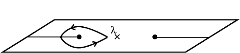
Figure 1: A closed path in the $\lambda$-plane for the ${\rm U}(2)$ theory. The bullets are at $\lambda=\pm 1$.

Formulas (2.11) and (2.12) are singular (non-analytic) for the special critical values (1.8) of $\lambda$. This has a very interesting consequence. Consider a closed path in the $\lambda$-plane, starting in the vicinity of the weakly coupled point $\lambda=0$, and going through one of the cut associated with the square roots in (2.11) or (2.12). We have depicted an example for ${\rm U}(2)$ in Figure 1. Because the square root picks a minus sign in this process, the vacua $|1\rangle$ and $|1\rangle^{\prime}$ are continuously deformed into one another when going along the path. More generally, the sheets of parameter space corresponding to the vacua $|k\rangle$ and $|k\rangle^{\prime}$ are connected through branch cuts originating at the singular points $\lambda=\lambda_{{\rm c},k}$. The structure of the parameter space is thus drastically changed by quantum effects. We will further discuss this kind of phenomenon in Section 3.

The model also has an interesting dependence in the bare $\theta$ angle. The transformation $\theta\rightarrow\theta+2\pi$, or equivalently $\Lambda_{\rm u}^{2}\rightarrow\Lambda_{\rm u}^{2}e^{2i\pi/N}$, amounts to a non-trivial monodromy among the vacua. Since the different vacua are physically inequivalent, this means that the physical correlation functions of the theory, which satisfy the cluster decomposition principle, are not $2\pi$ periodic in $\theta$. The same phenomenon was discussed in detail on a two dimensional model in [13].

2.2 Massless glueball

It is natural to guess that the non-analyticity at the critical values (1.8) is due to new degrees of freedom becoming massless. This is easily demonstrated in our case. If

$$\epsilon_{k}=1-\lambda/\lambda_{{\rm c},k}$$ (2.14)

denotes the deviation from the singular point, it is straightforward to show, by using (2.7), (2.9) and (2.10), that the glueball superpotential takes the following form for small $\epsilon_{k}$,

$$W(S)={2N\Lambda^{3}\over 3\lambda_{{\rm c},k}}-N\epsilon_{k}S+{N\lambda_{{\rm c},k}^{2}S^{3}\over 3\Lambda^{6}}+\cdots\,\raise 2.0pt\hbox{,}$$ (2.15)

where we have written only the most relevant terms. For $\epsilon_{k}=0$, $W(S)$ is critical. This implies, under a mild assumption of regularity for the Kähler potential, that we have a massless glueball. We could have used the superpotential (2.6) for $z$ as well. By introducing $\tilde{z}=z+m/(2g)$, we have

$${\cal W}^{(k)}={Nm^{3}\over 12g^{2}}-{Nm^{2}\epsilon_{k}\tilde{z}\over 4g}+{gN\tilde{z}^{3}\over 3}\,\cdotp$$ (2.16)

In the particular case we are considering, the superpotentials (2.15) and (2.16) give equally valid descriptions of the low energy physics. The variables $S$ and $z$ are on the same footing because the derivative $\partial_{z}\partial_{S}W_{\rm eff}$ of (2.3) is non-zero at the critical point, and thus both $S$ and $z$ mix with the massless degrees of freedom. As we will explain in Section 4.4, for more general critical points the fields $S$ and $z$ do not necessarily play symmetric rôles.

2.3 Confinement without a mass gap

The appearance of massless degrees of freedom in the confining regime of an ${\cal N}=1$ gauge theory is an interesting phenomenon. Note that the critical points found in the preceding subsection are such that the glueball condensate (2.11) vanishes,

$$\langle S\rangle_{\rm crit}=0\,.$$ (2.17)

If one considers, as was suggested in [14], that $\langle S\rangle$ is a good order parameter for confinement, equation (2.17) would imply that the theory no longer confines at the critical points. However, we are going to show that this interpretation is not correct in general. Indeed, we can calculate explicitly the monopole condensates at criticality, and we find

$$\langle M_{m}\tilde{M}_{m}\rangle_{k}=i\sqrt{2}g\Lambda_{\rm u}^{2}e^{2i\pi k/N}\sin{2\pi m\over N}\,\raise 2.0pt\hbox{,}\quad 1\leq m\leq N-1\,,\quad{\rm for}\ \lambda=\lambda_{{\rm c},k}\,.$$ (2.18)

This demonstrates that for $N$ odd we have a non zero string tension in all magnetic ${\rm U}(1)$ factors, and thus confinement without a mass gap. For $N$ even the condensate for $m=N/2$ vanishes, and thus the corresponding electric charges do not confine (in particular for ${\rm U}(2)$ we don’t have confinement at all). Those facts will be fully understood in Section 3.

To derive (2.18), we start from the equation obtained by extremizing the superpotential (2.1) with respect to the $u_{p}$s and the monopole fields. It is convenient to use the variables $x_{s}$ defined by

$$u_{p}={1\over p}\mathop{\rm tr}\nolimits\Phi^{p}={1\over p}\sum_{s=1}^{N}x_{s}^{p}\,.$$ (2.19)

We get

$$\sqrt{2}\sum_{m=1}^{N-1}{\partial A_{D,m}\over\partial x_{s}}\,\langle M_{m}\tilde{M}_{m}\rangle \!=\! -mx_{s}-gx_{s}^{2}\,,$$ (2.20)

$$A_{D,m} \!=\! 0\,.$$ (2.21)

As explained in [12], the variables $A_{D,m}$ are expressed in terms of period integrals

$$A_{D,m}=\oint_{\alpha_{m}}{x\,{\rm d}P\over 2i\pi y}$$ (2.22)

over the hyperelliptic curve

$$y^{2}=P(x)^{2}-4\Lambda_{\rm u}^{2N}=\prod_{s=1}^{N}(x-x_{s})^{2}-4\Lambda_{\rm u}^{2N}\,.$$ (2.23)

The contours $\alpha_{m}$ encircle the cuts that vanish when the condition (2.21) is satisfied. The calculation of $\partial A_{D,m}/\partial x_{s}$ was done in [15] in the ${\rm SU}(N)$ theory. The ${\rm U}(N)$ theory we are dealing with presently is only slightly more general. It is possible to use the ${\rm SU}(N)$ calculation by shifting the variables

$$x=\tilde{x}+z\,,\quad x_{s}=\tilde{x}_{s}+z\,,$$ (2.24)

where $z$ is defined in (2.2). The constraints (2.21) are solved in the $k^{\rm th}$ vacuum by adjusting

$$\tilde{x}_{s}=2\Lambda_{\rm u}e^{i\pi k/N}\cos{\pi(s-1/2)\over N}\,\raise 2.0pt\hbox{,}$$ (2.25)

which corresponds to $P=2(-1)^{k}\Lambda_{\rm u}^{N}\cos(Nt)$ for $\tilde{x}=2\Lambda_{\rm u}e^{i\pi k/N}\cos t$ [15]. It is then straightforward to show that

$${\partial A_{D,m}\over\partial z}=\oint_{\alpha_{m}}{{\rm d}P\over 2i\pi y}=\pm\oint_{\alpha_{m}}{N\,{\rm d}t\over 2\pi}=0\,.$$ (2.26)

The calculation of [15], Section 2, can then be repeated without change, yielding

$${\partial A_{D,m}\over\partial x_{s}}={i\sin\hat{t}_{m}\over N(\cos t_{s}-\cos\hat{t}_{m})}$$ (2.27)

for

$$t_{s}={\pi(s-1/2)\over N}\,\raise 2.0pt\hbox{,}\quad 1\leq s\leq N\,,\quad{\rm and}\quad\hat{t}_{m}={\pi m\over N}\,\raise 2.0pt\hbox{,}\quad 1\leq m\leq N-1\,.$$ (2.28)

The right hand side of (2.20) can be evaluated by using (2.24), (2.25) and (2.11),

$$-mx_{s}-gx_{s}^{2}=-2g\Lambda_{\rm u}^{2}e^{2i\pi k/N}\cos(2t_{s})\,.$$ (2.29)

The trigonometric identity derived in [15],

$$\sum_{m=1}^{N-1}{\sin\hat{t}_{m}\sin(q\hat{t}_{m})\over N(\cos t_{s}-\cos\hat{t}_{m})}=\cos(qt_{s})\,,\quad q\in{\mathbb{Z}}\,,$$ (2.30)

together with (2.20), (2.27) and (2.29), yields (2.18).

3 The quantum space of parameters

So far, we have adopted a purely field theoretical point of view. It is possible to gain further insights by studying the geometrical interpretation of our results, and in particular of the singular points on the space of parameters. A geometrical interpretation is possible because our model can be constructed in string theory by wrapping D5 branes on special two-cycles of a certain non-compact Calabi-Yau manifold [8]. At least as far as the calculation of F-terms is concerned, this geometry can be replaced by a dual geometry where the two-cycles go to three-cycles and Ramond-Ramond flux through those cycles takes the place of the D5 branes [8]. In theories with eight or more supercharges, the singularities are usually associated with the degeneration of some cycle in the geometry. Presently we are looking at a case with only four supercharges for which very little is known. For the theory (1.3), the non-trivial part of the CY geometry is a simple non-compact hyperelliptic complex curve given by an equation of the form

$$Y^{2}=W_{\rm tree}^{\prime}(x)^{2}-R(x)\,,$$ (3.1)

where $R(x)$ is a polynomial of degree $p-2$ if the tree-level superpotential $W_{\rm tree}$ is a polynomial of degree $p$. The three-cycles of the original CY space correspond to one-cycles encircling the branch cuts of the surface (3.1), and the non-zero RR fluxes are associated with non-zero period integrals of the differential form $Y{\rm d}x$. The $p-1$ free parameters in the polynomial $R(x)$ are then directly related to the fluxes through the $p-1$ cuts. A very useful way to look at the geometry (3.1) is to realize that it comes from the solution of the one matrix model with potential given by $W_{\rm tree}$ [9]. The distribution of flux through the cycles depends on the pattern of gauge symmetry breaking. The solution of the matrix model with $C$ non-trivial cuts is associated with an unbroken gauge group of the form ${\rm U}(N_{1})\times\cdots\times{\rm U}(N_{C})$. We have collected in the Appendix a set of useful results on the multi-cut matrix models that are relevant to this problem. In the main text we limit the discussion to the cubic $W_{\rm tree}$ (1.5).

3.1 One-cut solution

Let us start with the one-cut solution that corresponds to the vacua with unbroken gauge group that we have studied so far. The RR flux goes through one cycle only, and the other cycle is always degenerate. This means that the curve (3.1) takes the special form

$$Y^{2}=x^{2}(m+gx)^{2}-R(x)=M(x)^{2}(x-a)(x-b)\,.$$ (3.2)

The non-trivial period integral is (for conventions see the Appendix and in particular Figure 4; units are chosen such that $\Lambda_{\rm u}=1$)

$$\oint_{\gamma}Y\,{\rm d}x=-4i\pi S\,.$$ (3.3)

It is easy to show that

$$R(x)=4Sgx+{1\over 2}\delta(S/\delta+m)(3S/\delta+m)$$ (3.4)

where

$$\delta=(b-a)^{2}/16$$ (3.5)

is constrained by the condition (2.10). Unlike cases with ${\cal N}=2$ supersymmetry, the most general geometry consistent with the symmetries is not physical. The moduli are frozen by the condition that the effective superpotential is extremal. As derived in [10] (see also equations (A.29) and (A.30)), and consistently with the equation (2.9), this amounts to imposing an extremely simple condition,

$$\delta^{N}=1=\left({b-a\over 4}\right)^{2N}\,.$$ (3.6)

The fact that this condition depends on $W_{\rm tree}$ only through the position of the branch cuts $a$ and $b$ is a manifestation of the well-known universality of matrix models. As explained in the Appendix, this property remains true for any $W_{\rm tree}$ and an arbitrary number of cuts. Equation (3.6) shows that the non-trivial cycle of the physical curve can never vanish. This implies that the singular points (1.8), even though they are associated with a vanishing period integral (3.3) as stressed in (2.17), do not correspond to a vanishing cycle $\gamma$.

One may wonder whether the singular points correspond to the old Kazakov critical points of the matrix model [16, 7]. The Kazakov critical points occur when the root $x_{*}$ of the polynomial $M$ in (3.2) coincides with one of the branching points $a$ or $b$. By using (3.6), is it immediate to see that

$$x_{*}=-{m\over g}-{a+b\over 2}=-{m\over g}-\langle z\rangle\,,$$ (3.7)

where $\langle z\rangle=(a+b)/2$ is one of the $z$-field expectation values (2.11). The equation $x_{*}=a$ or $x_{*}=b$ is then solved when $\lambda$ goes to any of the $N$ values

$$\lambda_{{\rm Kazakov},k}={2\over 3}\,e^{-2i\pi k/N}\,,\quad 0\leq k\leq N-1\,.$$ (3.8)

Those are special values from the point of view of the matrix model, and thus also from the point of view of the superpotential $W(S)$, but are clearly different from the critical values (1.8). This comes from the fact that in gauge theory, only the solutions to $W^{\prime}(S)=0$ have a physical significance. This is very different from the ordinary matrix model where the condition $W^{\prime}=0$ has no meaning. In other words, the gauge theory critical points are obtained when the solutions to $W^{\prime}(S)=0$ are singular, and this condition is not related to the Kazakov condition of having $W$ singular.

It is not difficult to check that the genuine critical points (1.8) occur when the double point of (3.2) sits exactly in the middle of the cut,

$$x_{*}={a+b\over 2}\,\cdotp$$ (3.9)

This is a curious geometric condition that we will better understand in the next subsection.

3.2 Two-cut solution

3.2.1 General properties

The phases with broken gauge group ${\rm U}(N)\rightarrow{\rm U}(N_{1})\times{\rm U}(N_{2})$, $N_{1}\not=0$ and $N_{2}\not=0$, are described by the two-cut solution of the matrix model. A full discussion and the derivations of some technical results used in the following can be found in the Appendix. The curve (3.1) now takes the form

$$Y^{2}=g^{2}(x-a_{1})(x-b_{1})(x-a_{2})(x-b_{2})\,.$$ (3.10)

The branch cuts are chosen to run from $a_{1}$ to $b_{1}$ and from $a_{2}$ to $b_{2}$. The effective superpotential $W(S_{1},S_{2})$ can be calculated as a function of the fluxes through the two cuts. Upon extremization, we obtain two conditions (A.46) that the curve (3.10) must satisfy. Those conditions have $N_{1}N_{2}$ solutions corresponding to the vacua $|k_{1},k_{2};N_{1},N_{2}\rangle$, $0\leq k_{j}\leq N_{j}-1$, of the low energy ${\rm U}(N_{1})\times{\rm U}(N_{2})$ theory.

Interesting points on parameter space are those for which the curve (3.10) is singular. In the Appendix it is shown that the vanishing of an electric cycle (which occurs if one of the cuts shrinks to zero) is inconsistent with the conditions (A.46) except if $N_{1}$ or $N_{2}$ is zero, while the vanishing of the magnetic cycle (which occurs when the two cuts join) is possible if

$$k_{1}\equiv k_{2}\ {\rm mod}\ N_{1}\wedge N_{2}\,,$$ (3.11)

where $N_{1}\wedge N_{2}$ is the greatest common divisor of $N_{1}$ and $N_{2}$. In particular, if $N_{1}$ and $N_{2}$ are relatively prime, then all the vacua can have massless monopole points. The vanishing of the magnetic cycle implies that the electric coupling of the relative ${\rm U}(1)$ factor of the groups ${\rm U}(N_{1})$ and ${\rm U}(N_{2})$ blows up, or equivalently that the magnetic coupling vanishes. We then have a massless magnetically charged particle. Let us note that in both ${\cal N}=2$ and ${\cal N}=1$ gauge theories, a vanishing magnetic cycle is associated with a massless magnetically charged particle. However, when the cycle is non-vanishing, the mass of the monopole is exactly known only for ${\cal N}=2$ supersymmetry.

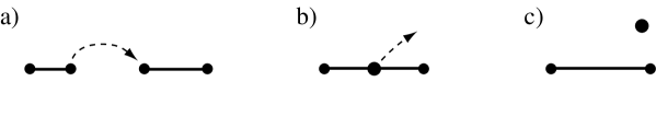
Figure 2: The transition from the two cut solution to the one cut solution (the inverse transition is of course possible as well). a) The endpoints of the two cuts get closer and eventually collide at the critical point, forming a double point. b) It is possible for the double point to move away from the cut. c) We are then left with the one-cut solution.

Another simple but important result proved in the Appendix is the following. Suppose that the parameters are adjusted in such a way that a curve extremizing the superpotential $W(S_{1},S_{2})$ has a vanishing magnetic cycle. This means that the two cuts have joined to form a single cut. Then the curve is also a solution of the extremization problem for the superpotential $W(S)$ relevant to the one-cut solution. Physically, this means that the ${\rm U}(N_{1})\times{\rm U}(N_{2})$ and ${\rm U}(N)$ branches touch at the massless monopole point. One can go from the broken to the unbroken phase by condensing the massless monopole and the mass gap is created by the usual magnetic Higgs mechanism. The geometry of the transition is depicted in Figure 2.

3.2.2 Examples

The above discussion implies that in addition to the massless glueball points discussed in Section 2, there will be many other singular points with massless monopoles on the branches of parameter space associated with the ${\rm U}(N)$ vacua $|k\rangle$ and $|k\rangle^{\prime}$. Those singularities are points of contact with the broken phases. The calculation of the monopole condensates in Section 2.3 actually suggests that for $N$ even the critical point (1.8) is such a point of contact, since we have found that the condensate $\langle M_{N/2}\tilde{M}_{N/2}\rangle_{k}$ vanishes. We would then have a massless monopole if $N$ is even in addition to the massless glueball that is present for any $N$.

It is actually not difficult to check this picture explicitly, and to discover that the relevant phase at $\lambda=\lambda_{\rm c}$ has ${\rm U}(N/2)\times{\rm U}(N/2)$ unbroken. To do so, let us note that there are $N^{2}/4$ vacua $|k_{1},k_{2};N/2,N/2\rangle$ for the ${\rm U}(N/2)\times{\rm U}(N/2)$ phase. The condition (3.11) is satisfied only in the vacua for which $k_{1}=k_{2}$. This implies that the curve (3.10) has a nice symmetry property that allows to solve the constraint (A.46) directly. The solution, derived in the Appendix, is

$$Y^{2}=x^{2}(m+gx)^{2}-4g^{2}e^{-4i\pi k/N}\Lambda_{\rm u}^{4}\,,\quad 0\leq k_{1}=k_{2}=k\leq N/2-1\,.$$ (3.12)

This solution can also be found by using the results of [8] and [17]. As stressed in [17], in the case $N=2$ the curve (3.12) exactly coincides with the Seiberg-Witten curve for ${\cal N}=2$ super Yang-Mills and gauge group ${\rm U}(2)$, with the moduli frozen to the classical values imposed by the tree-level superpotential. This means that there is an isomorphism in this particular case between the moduli space of ${\cal N}=2$ [12] and the parameter space of our ${\cal N}=1$ theory in the ${\rm U}(1)\times{\rm U}(1)$ phase. The monopole singularities are then nothing but the famous Seiberg-Witten singularities. For general even $N$, (3.12) degenerates precisely at the $N$ critical points (1.8), as we wished to prove. The branches for $|k\rangle$ and $|k\rangle^{\prime}$ touch the branch for $|k,k;N/2,N/2\rangle$ at $\lambda=\exp(-2i\pi k/N)$, and the branches for $|k+N/2\rangle$ and $|k+N/2\rangle^{\prime}$ touch the branch for $|k,k;N/2,N/2\rangle$ at $\lambda=-\exp(-2i\pi k/N)$.

It should be clear that the massless monopole singularities are not in general coinciding with (1.8). To illustrate this point, let us consider the ${\rm U}(3)$ theory. Since $N$ is odd we don’t expect to have a massless monopole for $\lambda=\lambda_{{\rm c},k}$, but on the other hand the condition (3.11) is satisfied for the broken ${\rm U}(2)\times{\rm U}(1)$ phase. It is easy to see what happens explicitly, because the solution can be found straightforwardly, for example by using the results of [8] and [17]. The curves for the vacua $|\eta,0;2,1\rangle$, $\eta=\pm 1$, where classically two eigenvalues are at zero and one is at $-m/g$, are given by

$$Y^{2}=(m+gx)(gx^{3}+mx^{2}+4\eta g\Lambda_{\rm u}^{3})\,.$$ (3.13)

A similar formula is valid for the vacua $|0,\eta;1,2\rangle$. The magnetic cycle of (3.13) vanishes when $\lambda$ goes to

$$\lambda_{{\rm U}(2)\times{\rm U}(1),k}={8\over 9}\,e^{-2i\pi k/3}\,,\quad 0\leq k\leq 2\,.$$ (3.14)

It is then straightforward to check that at criticality

$$\left({b_{2}-a_{1}\over 4}\right)^{2}=\delta=e^{2i\pi k/3}\,.$$ (3.15)

This is the correct condition for the one-cut phase. More precisely, we have a connection with the ${\rm U}(3)$ vacua $|k\rangle$ and $|k\rangle^{\prime}$ for $\lambda=\lambda_{{\rm U}(2)\times{\rm U}(1),k}$.

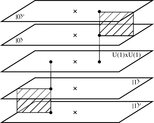
Figure 3: The five-sheeted structure of the parameter space for the ${\rm U}(2)$ gauge theory. The crosses denote the $\lambda=0$ point, and bullets represent singularities with massless glueball and monopole.

3.3 The quantum parameter space for ${\rm U}(2)$

As an illustration, we have depicted the full quantum space of parameters for the gauge group ${\rm U}(2)$ in Figure 3. The quantum parameter space is connected, whereas its classical counterpart would have three disconnected components by excluding the point $\lambda=\infty$. A similar picture would be valid for ${\rm U}(N)$ with $N$ even, the ${\rm U}(1)\times{\rm U(1)}$ phase being replaced by ${\rm U}(N/2)\times{\rm U}(N/2)$ in the $|k,k;N/2,N/2\rangle$ vacua, and $|0\rangle$, $|0\rangle^{\prime}$, $|1\rangle$, $|1\rangle^{\prime}$ being replaced by $|k\rangle$, $|k\rangle^{\prime}$, $|k+N/2\rangle$ and $|k+N/2\rangle^{\prime}$. There are also other components with various inter-connections in that case.

4 The large $N$ limit

4.1 Generalities

We can now tackle the problem that was the original motivation for this work. We have found non-trivial critical points for some particular values of the Higgs couplings. Following [1, 2], we would expect a non-trivial behaviour of the large $N$ expansion at the critical points. The only observables that we can calculate exactly are all related to the exact superpotentials discussed previously, or to the electric ${\rm U}(1)$ coupling $\tau$ in the broken phases. To be concrete, let us focus for the moment on the unbroken vacua and discuss the tensions of domain walls. The coupling $\tau$ will be discussed in section 4.3. The tension of a $(|p\rangle,|q\rangle)$ BPS domain wall interpolating between vacua $|p\rangle$ and $|q\rangle$ is simply given by [18]

$$T_{|p\rangle,|q\rangle}=|\tau_{|p\rangle,|q\rangle}|$$ (4.1)

where the complexified tension $\tau_{|p\rangle,|q\rangle}$ is defined by

$$\tau_{|p\rangle,|q\rangle}=N\left(\smash{W_{\rm low}^{|p\rangle}-W_{\rm low}^{|q\rangle}}\right)\,.$$ (4.2)

The factor of $N$ in (4.2) comes from the normalization of the $F$-term in (1.3). The standard lore about those domain walls is based on the analysis of the $g=0$ theory [11]. The tension is given in that case by

$$T_{|p\rangle,|q\rangle}=2N^{2}|\Lambda|^{3}\sin{\pi|p-q|\over N}\,\cdotp$$ (4.3)

The basic domain walls for which $|p-q|=1$, or more generally for which $|p-q|$ is of order one at large $N$, have a tension that scales as $N$ when $N\rightarrow\infty$,

$$T_{|p\rangle,|q\rangle}\mathrel{\mathop{\kern 0.0pt\sim}\limits_{N\rightarrow\infty}}2\pi N|p-q||\Lambda|^{3}\,.$$ (4.4)

This is consistent with a D-brane interpretation for the walls, with a closed string coupling constant of order $1/N$. It was indeed argued in [11] that the confining strings can end on the domain walls. More generally, with an arbitrary tree-level superpotential, the formula (4.4) is replaced by

$$\tau_{|p\rangle,|q\rangle}\mathrel{\mathop{\kern 0.0pt\sim}\limits_{N\rightarrow\infty}}2i\pi(p-q)\Lambda_{\rm u}^{2}\partial_{\Lambda_{\rm u}^{2}}W_{\rm low}=2i\pi N(p-q)\langle S\rangle\,,$$ (4.5)

where the expectation value is taken in any vacuum $|k\rangle$ for which $|k-p|$ is of order one (we will take $k=0$). The standard D-brane interpretation is thus valid as long as $\langle S\rangle\not=0$.

Points for which $\langle S\rangle=0$ are special from the point of view of large $N$, but are not necessarily associated with a breakdown of the $1/N$ expansion. For any even tree-level superpotential, it is actually very easy to adjust the parameters to get $\langle S\rangle=0$. For example, with

$$W_{\rm tree}(\Phi)={m\over 2}\,\Phi^{2}+{g_{4}\over 4}\,\Phi^{4}\,,$$ (4.6)

we have [10], in the vacua corresponding to $\langle\phi\rangle_{\rm cl}=0$,

$$\langle S\rangle=m\Lambda_{\rm u}^{2}e^{2i\pi k/N}+3g_{4}\Lambda_{\rm u}^{4}e^{4i\pi k/N}\,,$$ (4.7)

which is zero for

$$m=-3g_{4}\Lambda_{\rm u}^{2}e^{2i\pi k/N}\,.$$ (4.8)

The large $N$ expansion of the domain walls tensions is nevertheless perfectly well-behaved, starting at order $N^{0}$ for the special value (4.8). It is even very easy to get exactly tensionless $(|p\rangle,|q\rangle)$ domain walls, $W_{\rm low}^{|p\rangle}=W_{\rm low}^{|q\rangle}$, at finite $N$. By using the results of [10] it is straightforward to see that this happens for example for the theory (4.6) when

$$2m\sin{\pi(p-q)\over N}=-3g_{4}\Lambda_{\rm u}^{2}e^{i\pi(p+q)/N}\sin{2\pi(p-q)\over N}\,\cdotp$$ (4.9)

The condition (4.8) is recovered from the above equation in the large $N$ limit.

In our theory, in addition to the $(|p\rangle,|q\rangle)$ domain walls, we have $(|p\rangle^{\prime},|q\rangle^{\prime})$ domain walls with similar properties. More interestingly, there are also $(|p\rangle^{\prime},|q\rangle)$ domain walls. Those exist at the semi-classical level, unlike the $(|p\rangle,|q\rangle)$ walls that originate from chiral symmetry breaking. Their complexified tensions are simply given by

$$\tau_{|p\rangle^{\prime},|q\rangle}=N\left(\smash{W_{\rm low}^{|p\rangle^{\prime}}-W_{\rm low}^{|q\rangle}}\right).$$ (4.10)

In the semi-classical regime this is well approximated by

$$\tau_{|p\rangle^{\prime},|q\rangle}^{\rm cl}={N^{2}m^{3}\over 6g^{2}}\,\raise 2.0pt\hbox{,}$$ (4.11)

and scales as $N^{2}$ at large $N$. The $(|p\rangle^{\prime},|q\rangle)$ walls thus behave like closed string solitons (as opposed to D-branes). Remarkably, the results of Section 2 imply that the closed string solitons $(|p\rangle^{\prime},|q\rangle)$ and the D-branes $(|p\rangle,|q\rangle)$ or $(|p\rangle^{\prime},|q\rangle^{\prime})$ can be continuously deformed into one another by varying the parameters (see the discussion associated with Figure 1). This is reminiscent of the monodromy between magnetic monopoles and quarks in strongly coupled ${\cal N}=2$ gauge theories, as described explicitly for example in [19]. Moreover, the $(|k\rangle,|k\rangle^{\prime})$ domain wall is exactly tensionless at the critical value $\lambda=\lambda_{{\rm c},k}$ (1.8), as can be checked easily by using (2.12). The presence of a tensionless solitonic domain wall is an important feature of our critical point, and will be associated with a singular $1/N$ expansion.

4.2 Large $N$ and critical points

From (4.5) and (2.11), we have

$$\tau_{|p\rangle,|q\rangle}\mathrel{\mathop{\kern 0.0pt\sim}\limits_{N\rightarrow\infty}}2i\pi N(p-q)\Lambda^{3}\sqrt{1-\lambda}\,,$$ (4.12)

which generalizes (4.4) to arbitrary $\lambda$. The same formula up to a global minus sign is valid for $\tau_{|p\rangle^{\prime},|q\rangle^{\prime}}$, and from (2.12) we can also deduce

$$\tau_{|p\rangle^{\prime},|q\rangle}\mathrel{\mathop{\kern 0.0pt\sim}\limits_{N\rightarrow\infty}}{N^{2}m^{3}\over 6g^{2}}\,(1-\lambda)^{3/2}\,.$$ (4.13)

A well-behaved large $N$ expansion would then predict that $\tau_{|p\rangle,|q\rangle}$ and $\tau_{|p\rangle^{\prime},|q\rangle^{\prime}}$ are of order $N^{0}$ at $\lambda=\lambda_{\rm c}=1$, while $\tau_{|p\rangle^{\prime},|q\rangle}$ would be of order $N$, but this is not what happens. The exact formulas show that

$$\tau_{|p\rangle,|q\rangle}\mathrel{\mathop{\kern 0.0pt\sim}\limits_{N\rightarrow\infty}}{2^{5/2}\pi^{3/2}e^{i\pi/4}\over 3}\Lambda^{3}\sqrt{N}\left(q^{3/2}-p^{3/2}\right)\,,$$ (4.14)

$$\tau_{|p\rangle^{\prime},|q\rangle}\mathrel{\mathop{\kern 0.0pt\sim}\limits_{N\rightarrow\infty}}{2^{5/2}\pi^{3/2}e^{i\pi/4}\over 3}\Lambda^{3}\sqrt{N}\left(q^{3/2}+p^{3/2}\right)\,,$$ (4.15)

at criticality. The common $\sqrt{N}$ dependence for the “soliton” and the “D-brane” is remarkable and signals the breakdown of the $1/N$ expansion near $\lambda=\lambda_{\rm c}$. It is straightforward to compute the $1/N$ corrections to (4.12) or (4.13) for $\lambda\not=\lambda_{\rm c}$,

$$\hskip-48.36958pt\tau_{|p\rangle,|q\rangle}=2i\pi N(p-q)\Lambda^{3}\sqrt{1-\lambda}\Biggl{[}1+{i\pi(2-3\lambda)(p+q)\over 2(1-\lambda)N}+{\cal O}\left(1/(N(1-\lambda))^{2}\right)\Biggr{]},$$ (4.16)

$$\hskip-48.36958pt\tau_{|p\rangle,|q\rangle^{\prime}}={N^{2}m^{3}\over 6g^{2}}\,(1-\lambda)^{3/2}\Biggl{[}1-{3i\pi\lambda(p+q)\over 2(1-\lambda)N}+{\cal O}\left(1/(N(1-\lambda))^{2}\right)\Biggr{]}\,.$$ (4.17)

The expansions (4.16) and (4.17) are singular at $\lambda=1$ as expected.

4.3 The double scaling limit

The formulas (4.16) and (4.17) are extremely suggestive. The divergences at $\lambda=1$ are very specific, and can be compensated for by taking $N\rightarrow\infty$ and $\lambda\rightarrow\lambda_{\rm c}=1$ in a correlated way given in (1.9). The rescaled tensions

$$t_{|p\rangle,|q\rangle}=\sqrt{1-\lambda}\,\tau_{|p\rangle,|q\rangle}\,,\quad t_{|p\rangle^{\prime},|q\rangle}=\sqrt{1-\lambda}\,\tau_{|p\rangle^{\prime},|q\rangle}$$ (4.18)

then go to finite universal limits

$$t_{|p\rangle,|q\rangle}^{\rm scaled}={2\Lambda^{3}\over 3\kappa^{2}}\Bigl{[}\left(1-2i\pi q\kappa\right)^{3/2}-\left(1-2i\pi p\kappa\right)^{3/2}\Bigr{]}\,,$$ (4.19)

$$t_{|p\rangle^{\prime},|q\rangle}^{\rm scaled}={2\Lambda^{3}\over 3\kappa^{2}}\Bigl{[}\left(1-2i\pi q\kappa\right)^{3/2}+\left(1-2i\pi p\kappa\right)^{3/2}\Bigr{]}\,.$$ (4.20)

In the scaling (1.9), it is natural to conjecture that the original gauge theory reduces to a four dimensional non-critical string theory, or, equivalently, to a five dimensional critical string theory. Equations (4.19) and (4.20) are interpreted as giving the exact tensions for BPS D2-branes and solitonic two-branes in this string theory. The rescaling (4.18) corresponds to a renormalization in the world-sheet theory. A detailed discussion of this conjecture can be found in [3, 4, 6], and it will not be repeated here. As explained in the introduction, the idea is simply to generalize the old matrix model approach to non-critical strings [7, 20]. Note that by going through the branch cuts in equations (4.19) or (4.20), we can transform continuously a D-brane (whose tension goes like $1/\kappa$ at weak coupling) into a soliton (whose tension goes like $1/\kappa^{2}$ at weak coupling), and vice-versa.

We have emphasized in section 3.1 that the critical points (1.8) of the gauge theory are not the same as the critical points of the one-cut matrix model. On the other hand, for $N$ even, the critical points are also seen in the two-cut matrix model, and there they do correspond to a regime that was used to describe the $c=1$ strings [21, 22]. We would like to stress that this fact is, as far as we can see, of no deep significance in the present context. It does mean that large Feynman graphs dominate near the critical points. This is perfectly consistent with the four dimensional path integral picture sketched in the introduction because the matrix model planar diagrams are related to gauge theory planar diagrams [9]. However, the size $N$ of matrices in the gauge theory path integral is not related to the size $n$ of matrices in the matrix model. In particular, the scaling (1.9) relevant to the gauge theory is not the same as the scaling relevant to the $c=1$ matrix model that was worked out long ago in [23] (four dimensional scalings reminiscent of the $c=1$ scaling do occur [3], but in different cases). The crucial point is that the double scaling limit (1.9) yields a four dimensional non-critical (or five dimensional critical) string, because the starting point is a four dimensional path integral. This is very different from the $c=1$ string. The gauge theory path integral being non-perturbatively defined, the scaling provides a full non-perturbative definition of the resulting string theory. Again this is in sharp contrast with the $c=1$ string case.

By using (3.12), (A.37) and (A.38), it is easy to study the scaling of the ${\rm U}(1)$ coupling $\tau_{p}$ of the $|p,p;N/2,N/2\rangle$ vacua. It is actually convenient to work with the dual magnetic coupling

$$\tau_{p,\rm D}=-1/\tau_{p}\,.$$ (4.21)

The parameter $k^{\prime 2}$ of the curve (3.12) goes to

$$k^{\prime 2}\longrightarrow 2\sqrt{2}\sqrt{1-\lambda}\sqrt{1-2i\pi p\kappa}$$ (4.22)

in the scaling (1.9). The renormalized coupling

$$t_{p,\rm D}=\tau_{p,\rm D}-{i\over\pi}\ln{\sqrt{1-\lambda}\over 4\sqrt{2}}$$ (4.23)

then goes to a finite limit

$$t_{p,\rm D}^{\rm scaled}={i\over 2\pi}\ln(1-2i\pi p\kappa)\,.$$ (4.24)

There is a subtle difference between the double scaling limit yielding (4.19), (4.20) or (4.24) and the double scaling limits discussed in previous papers [3, 4, 6]. Even though equations (4.12) or (4.13) clearly shows that the divergences encountered in $1/N$ corrections have an IR origin, the world-sheet renormalizations (4.18), whose form are dictated by the $N$ dependence of $\tau_{|p\rangle,|q\rangle}$ and $\tau_{|p\rangle^{\prime},|q\rangle}$, correspond to a UV limit in space-time.

4.4 Multicritical points

Let us sketch an elementary field theoretic discussion of more general critical points. A systematic study can certainly be done by using the ideas described in Section 3, but this is beyond the scope of the present paper. Let us consider an arbitrary tree level superpotential of degree $p$,

$$W_{\rm tree}(\Phi)=\sum_{r=1}^{p}{g_{r}\over r}\,\Phi^{r}\,.$$ (4.25)

Classically, the theory has generically $p-1$ independent vacua with unbroken gauge group, labeled by an integer $J$. Our goal is to construct multicritical points akin to the one studied in Section 2.

A first important step is to understand the distinction between the variable $z=(\mathop{\rm tr}\nolimits\phi)/N$, which is natural from the UV, ${\cal N}=2$ point of view, and the glueball field $S$, which is more natural from the IR, ${\cal N}=1$ point of view. There are $N$ superpotentials for $z$, each of degree $p$, and labeled by an integer $k$. The formula generalizing (2.6) to the case of (4.25) was derived in [10] and reads

$${\cal W}^{(k)}(z)=N\sum_{r\geq 0}\omega_{r}^{(k)}z^{r}\,,$$ (4.26)

where

$$\omega_{r}^{(k)}=\sum_{q\geq 0}{g_{r+2q}\over r+2q}{\rm C}_{r+2q}^{2q}{\rm C}_{2q}^{q}\Lambda_{\rm u}^{2q}e^{2i\pi kq/N}\,.$$ (4.27)

The equation ${\cal W}^{(k)^{\prime}}(z)=0$ has $p-1$ solutions, corresponding to the $p-1$ classical vacua. It is impossible, by considering a given superpotential for $z$ (or for any of the fields $\mathop{\rm tr}\nolimits\phi^{r}$), to derive the existence of $N$ vacua associated with each of the $p-1$ classical vacua. This is in sharp contrast with the superpotentials for the field $S$. There are $p-1$ of them, that we denote $W_{(J)}(S)$, $0\leq J\leq p-2$. Each of the equations $W_{(J)}^{\prime}(S)=0$ has precisely $N$ solutions, reflecting chiral symmetry breaking in the pure ${\cal N}=1$ theory.

Critical points of any order for the field $z$ can be straightforwardly obtained. For example, formulas (4.26) and (4.27) imply that we have a critical point of order $\ell$ at $z=0$ when the $g_{r}$s are such that $\omega_{r}^{(k)}=0$ for $1\leq r\leq\ell$. However, it is important to realize that an $\ell^{\rm th}$ order critical point of ${\cal W}^{(k)}(z)$ does not necessarily correspond to an $\ell^{\rm th}$ order critical point for a corresponding glueball superpotential $W_{(J)}(S)$. Let us give a concrete example based on the tree-level superpotential (4.6), which yields

$${\cal W}^{(k)}(z)=Nm\Lambda_{\rm u}^{2}e^{2i\pi k/N}+{3N\over 2}\,g_{4}\Lambda_{\rm u}^{4}e^{4i\pi k/N}+{N\over 2}\left(m+6g_{4}\Lambda_{\rm u}^{2}e^{2i\pi k/N}\right)z^{2}+{Ng_{4}z^{4}\over 4}\,\cdotp$$ (4.28)

There are $3N$ vacua with unbroken gauge group, denoted by $|k\rangle^{J}$, $0\leq J\leq 2$, $0\leq k\leq N-1$, for which

$$\hskip-19.91684pt\langle S\rangle_{|k\rangle^{0}}=m\Lambda_{\rm u}^{2}e^{2i\pi k/N}+3g_{4}\Lambda_{\rm u}^{4}e^{4i\pi k/N}\,,\quad\langle z\rangle_{|k\rangle^{0}}=0\,,$$ (4.29)

$$\hskip-19.91684pt\langle S\rangle_{|k\rangle^{1}}=-2m\Lambda_{\rm u}^{2}e^{2i\pi k/N}-15g_{4}\Lambda_{\rm u}^{4}e^{4i\pi k/N}\,,\quad\!\!\langle z\rangle_{|k\rangle^{1}}=i\Bigl{(}{m\over g_{4}}\Bigr{)}^{1/2}\Bigl{(}1+{6g_{4}\Lambda_{\rm u}^{2}e^{2i\pi k/N}\over m}\Bigr{)}^{1/2}\!,$$

$$\hskip-19.91684pt\langle S\rangle_{|k\rangle^{2}}=-2m\Lambda_{\rm u}^{2}e^{2i\pi k/N}-15g_{4}\Lambda_{\rm u}^{4}e^{4i\pi k/N}\,,\quad\!\!\langle z\rangle_{|k\rangle^{2}}=-i\Bigl{(}{m\over g_{4}}\Bigr{)}^{1/2}\Bigl{(}1+{6g_{4}\Lambda_{\rm u}^{2}e^{2i\pi k/N}\over m}\Bigr{)}^{1/2}\!\!\!.$$

There is a critical point for ${\cal W}^{(k)}(z)$ when $m=-6g_{4}\Lambda_{\rm u}^{2}e^{2i\pi k/N}$. The field $z$ is then massless in the vacua $|k\rangle^{J}$, for any $J$. On the other hand, it is straightforward to check, by using the results in [10], that the superpotentials $W_{(J)}(S)$ are not critical, and thus we do not have a massless glueball. The non-trivial phenomena described in the present paper, like the breakdown of the large $N$ expansion, only occur in the vacua with massless glueballs. For the other critical points, the large $N$ expansion is perfectly well-behaved.

Multicritical points associated with a singular large $N$ expansion can be obtained by considering a general odd tree-level superpotential. When only $g_{1}$ and $g_{3}$ are turned on, the critical point at $z=0$ for $g_{1}=-2g_{3}\Lambda_{\rm u}^{2}$ is in the same universality class as (1.8). If we turn on $g_{5}$, we can go to a higher critical point for $g_{1}=18\Lambda_{\rm u}^{4}e^{4i\pi k/N}g_{5}$ and $g_{3}=-12\Lambda_{\rm u}^{2}e^{2i\pi k/N}g_{5}$. We then have ${\cal W}^{(k)}(z)=Ng_{5}z^{5}/5$. We have checked explicitly using results in [10] that the superpotential for the glueball superfield also goes like $S^{5}$ at criticality. The tension of the domain walls then goes like $N^{3/4}$ at large $N$. The same construction starting with an odd $W_{\rm tree}$ of degree $2\ell+1$ presumably yields similar critical points with ${\cal W}(z)\propto z^{2\ell+1}$ and $W(S)\propto S^{2\ell+1}$. The large $N$ tension at criticality scales as

$$T(\ell)\propto N^{1-1/(2\ell)}\,,$$ (4.30)

and double scaling limits can certainly be defined. It would be nice to work out those multicritical points and the associated double scaling limits more explicitly.

5 Conclusion and prospects

Non-trivial exact ${\cal N}=1$ effective superpotentials have proven to be extremely powerful tools to work out some new interesting physics in strongly coupled ${\cal N}=1$ gauge theories. There is a qualitative similarity with ${\cal N}=2$ gauge theories, the parameter space replacing the moduli space. There are also some fundamental differences. For example, the singularities are not necessarily associated with vanishing cycles in the geometric description, and extended objects play an important rôle. It would be nice to understand the general structure of the quantum space of parameters for an arbitrary polynomial $W_{\rm tree}$, and in particular to study higher critical points à la Argyres-Douglas.

The matrix model proposal made in [9] can in principle be used to study a wide class of examples, and we are presently working on the theory with two adjoint Higgs fields. One of the motivations to study such a model is that it is not a simple deformation of a theory with extended supersymmetry, unlike all the cases that have been worked out for the moment [9, 10, 24].

Maybe the most important message of this paper is that the old matrix model approach to non-critical strings can be generalized to four dimensional theories with ${\cal N}=1$ supersymmetry. This is a new and very important example where the ideas advocated in [1, 2, 3, 4, 5, 6] apply. The results for ${\cal N}=2$ obtained in [3] actually apply in ${\cal N}=1$ with a degree $N$ tree-level superpotential. The parameter space for the phase with maximal gauge symmetry breaking ${\rm U}(N)\rightarrow{\rm U}(1)^{N}$ is indeed isomorphic to the ${\cal N}=2$ moduli space [17]. It seems that much could be learned on four dimensional non-critical strings in this way. Only very few results are available, and we believe that it will be extremely rewarding to work out the general structure behind the four dimensional double scaling limits. The study of gauge theories with adjoint Higgs fields in two or three dimensions, and the associated critical points and double scaling limits, could also be potentially very interesting.

Acknowledgements

This work was initiated thank’s to Robbert Dijkgraaf inspiring talk at the Strings 2002 conference in Cambridge, UK. I am also indebted to Edward Witten for suggesting that the classical vacua $\langle\phi\rangle_{\rm cl}=0$ and $\langle\phi\rangle_{\rm cl}=-m/g$ may mix at strong coupling. I would also like to acknowledge many useful discussions with J.-P. Derendinger, R. Hernández, T. Hollowood, K. Intriligator, N. Seiberg and V. Kazakov. This work was supported in part by the Swiss National Science Foundation.

Appendix: The multi-cut solutions

1 Generalities

Let us imagine that we are considering the theory (1.3) with an arbitrary polynomial tree-level superpotential of degree $p$

$$W_{\rm tree}(\phi)=\sum_{r=1}^{p}{g_{r}\over r}\,\phi^{r}\,.$$ (A.1)

The most general gauge symmetry breaking pattern is of the form ${\rm U}(N)\rightarrow{\rm U}(N_{1})\times\cdots\times{\rm U}(N_{C})$, with $N_{1}+\cdots+N_{C}=N$ and $C\leq p-1$. The quantum effective superpotential is expressed in such a vacuum in terms of a $N_{k}$-independent prepotential ${\cal F}$ as

$$W=-\sum_{k=1}^{C}N_{k}\partial_{S_{k}}{\cal F}\,.$$ (A.2)

The prepotential is given by the planar approximation to a holomorphic integral over complex $n\times n$ matrices [9],

$$\exp\left(n^{2}{\cal F}/S^{2}\right)=\int_{\rm planar}\hskip-14.22636pt{\rm d}^{n^{2}}\phi\,\exp\Bigl{[}-{n\over S}\mathop{\rm tr}\nolimits W_{\rm tree}(\phi)\Bigr{]}\,,$$ (A.3)

where we are working in units for which $\Lambda_{\rm u}=1$. We can restrict ourselves to hermitian matrices and real couplings to compute (A.3) because there is no ambiguity in the analytic continuation for planar diagrams. The eigenvalue distribution $\rho(x)$ has a support

$${\rm Support}[\rho]=\bigcup_{k=1}^{C}[a_{k},b_{k}]$$ (A.4)

on $C$ cuts $[a_{k},b_{k}]$ which classically shrink to points that coincide with $C$ distinct roots of the equation $W_{\rm tree}^{\prime}(x)=0$. The prepotential

$${\cal F}=-S\int\!{\rm d}x\,\rho(x)W_{\rm tree}(x)+S^{2}\int\!{\rm d}x{\rm d}z\,\rho(x)\rho(z)\ln|x-z|\,,$$ (A.5)

as well as the superpotential $W$, depend on the filling fractions

$${S_{k}\over S}=\int_{a_{k}}^{b_{k}}\rho(x)\,{\rm d}x$$ (A.6)

that must be kept fixed in the integral (A.3). The filling fractions satisfy the constraint

$$\sum_{k=1}^{C}S_{k}=S\,.$$ (A.7)

It is very convenient to introduce

$$\omega(x)=\int_{-\infty}^{+\infty}{\rho(z)\,{\rm d}z\over x-z}\,\raise 2.0pt\hbox{,}$$ (A.8)

in terms of which

$$\rho(x)={i\over 2\pi}\left(\omega(x+i\epsilon)-\omega(x-i\epsilon)\right)\,.$$ (A.9)

The fundamental saddle point equation reads

$$W_{\rm tree}^{\prime}(x)=S\left(\omega(x+i\epsilon)+\omega(x-i\epsilon)\right)\quad{\rm for}\quad x\in{\rm Support}\,[\rho]\,.$$ (A.10)

The force acting on a test eigenvalue at $x$ is deduced from (A.5) to be $-nY(x)/S$ where

$$Y(x)=W_{\rm tree}^{\prime}(x)-2S\omega(x)\,.$$ (A.11)

One can show using (A.10) that $Y(x)$ satisfies an algebraic equation [20]

$$Y^{2}=W_{\rm tree}^{\prime}(x)^{2}-R(x)=M(x)^{2}\prod_{k=1}^{C}(x-a_{k})(x-b_{k})\,,$$ (A.12)

where

$$R(x)=4Sg_{p}x^{p-2}+\cdots$$ (A.13)

is a polynomial of degree $p-2$ and $M$ is a polynomial of degree $p-1-C$. The coefficients of $R$ are fixed in terms of the $S_{k}$ by the conditions (A.6) which can be conveniently rewritten

$$\oint_{\gamma_{k}}Y\,{\rm d}x=-4i\pi S_{k}\,.$$ (A.14)

The definition of various contours is given in Figure 4.

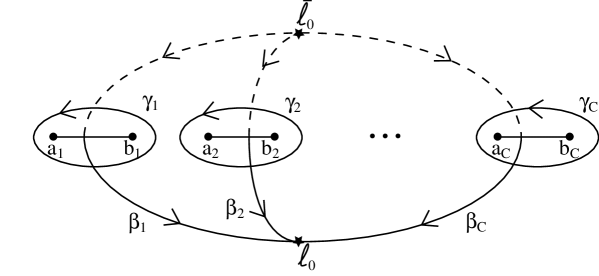
Figure 4: Definition of the contours $\gamma_{k}$ and $\beta_{k}$ used in the text (similar definitions were given in [17]). The points $\ell_{0}$ and $\bar{\ell}_{0}$ are going to infinity on the upper and lower sheets of the non-compact Riemann surface (A.19). As a consequence, the contours $\beta_{k}$ are not closed.

Since we are interested in the derivatives of $\cal F$ to compute the superpotential (A.2), it is very useful to introduce

$$\psi_{k}(x)={\partial(S\omega)\over\partial S_{k}}=-{1\over 2}{\partial Y\over\partial S_{k}}\,\cdotp$$ (A.15)

Equation (A.10) implies that

$$\psi_{k}(x+i\epsilon)+\psi_{k}(x-i\epsilon)=0\quad{\rm for}\quad x\in{\rm Support}\,[\rho]\,,$$ (A.16)

and (A.11) and (A.14) imply that

$${1\over 2i\pi}\oint_{\gamma_{l}}\psi_{k}(x)\,{\rm d}x=\delta_{k,l}\,.$$ (A.17)

The asymptotics at infinity of $\psi_{k}$ are deduced from the corresponding asymptotics $\omega(x)\sim 1/x$ and (A.15),

$$\psi_{k}(x)\mathrel{\mathop{\kern 0.0pt\sim}\limits_{x\rightarrow\infty}}{1\over x}\,\cdotp$$ (A.18)

These results prove that the differentials $\psi_{k}{\rm d}x$ form a canonical basis of $\log$-normalizable holomorphic one-forms on the genus $C-1$ non-compact Riemann surface

$$y^{2}=\prod_{k=1}^{C}(x-a_{k})(x-b_{k})\,.$$ (A.19)

Note that the polynomial $M$ in (A.12) no longer appears. This simplification is at the origin of “universality” in our problem: the derivatives of $W$ will depend on $W_{\rm tree}$ only through the branching points $a_{k}$ and $b_{k}$. We can write explicitly

$$\psi_{k}(x)={N_{k}(x)\over y}\,\raise 2.0pt\hbox{,}$$ (A.20)

where

$$N_{k}(x)=x^{C-1}+\cdots$$ (A.21)

is a polynomial of degree $C-1$ whose coefficients are determined by the equations (A.17). From (A.20), (A.15) and (A.9), one then obtains

$${\partial(S\rho)\over\partial S_{k}}=\left\{\matrix{{\displaystyle N_{k}(x)\over\displaystyle\pi\sqrt{(x-a_{q})(b_{q}-x)\smash{\prod_{k\not=q}}(x-a_{k})(x-b_{k})}}\quad&{\rm for}\ x\in[a_{q},b_{q}]\,,\cr&\cr&\cr 0\quad&{\rm for}\ x\notin{\rm Support}[\rho]\,.\cr}\right.$$ (A.22)

This equation can be used to compute the derivatives of $\cal F$, generalizing a calculation made in the Appendix of [10]. The first derivatives of $\cal F$ can also be obtained by noting that adding an eigenvalue to the $k^{\rm th}$ cut mimics the variation $\delta S_{k}=S/n$ [9]. By taking into account the energy cost in creating the eigenvalue at infinity, we then obtain

$$\partial_{S_{k}}{\cal F}=\lim_{\ell_{0}\rightarrow\infty}\Bigl{(}{1\over 2}\int_{\beta_{k}}Y\,{\rm d}x+2S\ln\ell_{0}-W_{\rm tree}(\ell_{0})\Bigr{)}\,,$$ (A.23)

where the contours $\beta_{k}$ are defined in Figure 4. By using (A.15) we deduce

$$\partial_{S_{k}}\partial_{S_{l}}{\cal F}=-2i\pi t_{kl}$$ (A.24)

or equivalently

$$\partial_{S_{k}}W=2i\pi\sum_{l=1}^{C}N_{l}\,t_{kl}\,,$$ (A.25)

where $t_{kl}$ is the regularized “period” matrix of the non-compact curve (A.19),

$$t_{kl}=\lim_{\ell_{0}\rightarrow\infty}\Bigl{(}{1\over 2i\pi}\int_{\beta_{l}}\psi_{k}\,{\rm d}x+{i\over\pi}\ln\ell_{0}\Bigr{)}=t_{lk}\,.$$ (A.26)

By using the normalizations (A.17), it is straightforward to show that the trivial exchange of the endpoints of the $k^{\rm th}$ cut amounts to the transformation $t_{kk}\rightarrow t_{kk}+1$. By taking into account this identification, we obtain that the conditions for a critical point of $W$ are

$$\sum_{l=1}^{C}N_{l}t_{jl}\equiv k_{j}\ {\rm mod}\ N_{j}\,,\quad 1\leq j\leq C\,.$$ (A.27)

There are $\prod_{j=1}^{C}N_{j}$ solutions to (A.27), labeled by the ${\mathbb{Z}}_{N_{j}}$-valued numbers $k_{j}$. As already mentioned, an important property of (A.27) is that it depends on $W_{\rm tree}$ only through the positions of the branch cuts of the curve (A.19).

2 Applications

2.1 One-cut solution

In the one cut case, there are only two branching points $a_{1}=a$ and $b_{1}=b$, and the holomorphic one-form is

$$\psi\,{\rm d}x={{\rm d}x\over\sqrt{(x-a)(x-b)}}\,\cdotp$$ (A.28)

The only period is

$$t_{11}=\lim_{\ell_{0}\rightarrow\infty}\Bigl{(}{1\over i\pi}\int_{b}^{\ell_{0}}{{\rm d}x\over\sqrt{(x-a)(x-b)}}+{i\over\pi}\ln\ell_{0}\Bigr{)}={i\over\pi}\ln{b-a\over 4}\,\raise 2.0pt\hbox{,}$$ (A.29)

and the physical condition (A.27) is

$$Nt_{11}\equiv k\ {\rm mod}\ N\,.$$ (A.30)

We thus find again (3.6).

2.2 Two-cut solution

We limit the discussion below to the two-cut solution ${\rm U}(N)\rightarrow{\rm U}(N_{1})\times{\rm U}(N_{2})$, $N_{1}\not=0$ and $N_{2}\not=0$, because this is the case used in the main text, but most of the arguments can be generalized straightforwardly to any number of cuts. It is convenient to introduce the cycles $\alpha$ and $\gamma$ defined by

$$\alpha=\beta_{1}-\beta_{2}\,,\quad\gamma=\gamma_{1}+\gamma_{2}\,.$$ (A.31)

Simple identities are

$$\oint_{\gamma}{{\rm d}x\over y}=0\,,\quad\oint_{\gamma}{x\,{\rm d}x\over y}=2i\pi\,.$$ (A.32)

The basis of $\log$-normalizable holomorphic one-forms is

$$\psi_{1}\,{\rm d}x={x+\mu_{1}\over y}\,{\rm d}x\,,\quad\psi_{2}\,{\rm d}x={x+\mu_{2}\over y}\,{\rm d}x\,.$$ (A.33)

By using (A.32) and $t_{12}=t_{21}$ one can derive the set of useful formulas

$$\mu_{2}-\mu_{1}={2i\pi\over\oint_{\gamma_{2}}{\rm d}x/y}={\pi\sqrt{(b_{2}-b_{1})(a_{2}-a_{1})}\over 2K(k)}\,\raise 2.0pt\hbox{,}$$ (A.34)

$$\mu_{1}\oint_{\alpha}{{\rm d}x\over y}=(\mu_{1}-\mu_{2})\int_{\beta_{1}}{{\rm d}x\over y}-\oint_{\alpha}{x\,{\rm d}x\over y}\,\raise 2.0pt\hbox{,}$$ (A.35)

$$\mu_{2}\oint_{\alpha}{{\rm d}x\over y}=(\mu_{1}-\mu_{2})\int_{\beta_{2}}{{\rm d}x\over y}-\oint_{\alpha}{x\,{\rm d}x\over y}\,\raise 2.0pt\hbox{,}$$ (A.36)

$$2t_{12}-t_{11}-t_{22}=\tau={\oint_{\alpha}{\rm d}x/y\over\oint_{\gamma_{2}}{\rm d}x/y}={iK(k^{\prime})\over K(k)}\,\raise 2.0pt\hbox{,}$$ (A.37)

where $K$ is the standard complete elliptic integral of the first kind and

$$k^{2}={(b_{2}-a_{2})(b_{1}-a_{1})\over(b_{2}-b_{1})(a_{2}-a_{1})}\,\raise 2.0pt\hbox{,}\quad k^{\prime 2}=1-k^{2}={(a_{2}-b_{1})(b_{2}-a_{1})\over(b_{2}-b_{1})(a_{2}-a_{1})}\,\cdotp$$ (A.38)

The parameter $\tau$ in (A.37) is the modular parameter of the compact part of the curve (A.19). Physically it corresponds to the non-trivial electric coupling constant of the relative ${\rm U}(1)$ factor $(N_{2}\times{\rm U}(1)_{1}-N_{1}\times{\rm U}(1)_{2})/N$ of the ${\rm U}(N_{1})$ and ${\rm U}(N_{2})$ groups, where ${\rm U}(1)_{j}\subset{\rm U}(N_{j})$.

Interesting physics is potentially associated with a singular curve, and it is important to understand how the periods of the smooth curve behave in the limit in which one of the cycle vanishes. Let us first consider the case of a vanishing electric cycle, for example $\gamma_{1}\rightarrow 0$. In the limit, we have $a_{1}=b_{1}=a$, and

$$\lim_{\gamma_{1}\rightarrow 0}\oint_{\gamma_{1}}{{\rm d}x\over y}={2i\pi\over\sqrt{(a_{2}-a)(b_{2}-a)}}\,\raise 2.0pt\hbox{,}\quad\lim_{\gamma_{1}\rightarrow 0}\oint_{\gamma_{1}}{x\,{\rm d}x\over y}={2i\pi a\over\sqrt{(a_{2}-a)(b_{2}-a)}}\,\cdotp$$ (A.39)

From those equations we deduce

$$\mu_{1}=-a+\sqrt{(a_{2}-a)(b_{2}-a)}\,,\quad\mu_{2}=-a\,.$$ (A.40)

One then shows immediately that the periods for the singular curve are

$$t_{22}={i\over\pi}\ln{b_{2}-a_{2}\over 4}\,\raise 2.0pt\hbox{,}\quad t_{12}={i\over\pi}\ln{b_{2}-a_{2}\over 4}{\sqrt{b_{2}-a}-\sqrt{a_{2}-a}\over\sqrt{b_{2}-a}+\sqrt{a_{2}-a}}\,\raise 2.0pt\hbox{,}\quad t_{11}=\infty\,.$$ (A.41)

The divergence of $t_{11}$ is directly related to the vanishing of the electric coupling constant. Let us now consider the physically more interesting case of a vanishing magnetic cycle $\alpha\rightarrow 0$. We have $a_{2}=b_{1}=c$ in the limit, and we will then note $a_{1}=a$ and $b_{2}=b$. Formulas similar to (A.39) are

$$\lim_{\alpha\rightarrow 0}\oint_{\alpha}{{\rm d}x\over y}={2\pi\over\sqrt{(c-a)(b-c)}}\,\raise 2.0pt\hbox{,}\quad\lim_{\alpha\rightarrow 0}\oint_{\alpha}{x\,{\rm d}x\over y}={2\pi c\over\sqrt{(c-a)(b-c)}}\,\cdotp$$ (A.42)

Moreover, $\oint_{\gamma_{2}}{\rm d}x/y$ diverges. This is equivalent to the vanishing of $\tau$ or of the magnetic coupling. Equations (A.34), (A.35) and (A.36) then imply

$$\mu_{1}=\mu_{2}=-c\,.$$ (A.43)

For the singular curve we thus have

$$\psi_{1}=\psi_{2}={1\over\sqrt{x-a)(x-b)}}=\psi\,,$$ (A.44)

and we immediately deduce

$$t_{11}=t_{22}=t_{12}={i\over\pi}\ln{b-a\over 4}\,\cdotp$$ (A.45)

The equations (A.44) and (A.45) coincide nicely with the corresponding equations (A.28) and (A.29) for the one-cut case.

The physical curves are characterized by the conditions (A.27) which read in the present case

$$N_{1}t_{11}+N_{2}t_{12}\equiv k_{1}\ {\rm mod}\ N_{1}\,,\quad N_{2}t_{22}+N_{1}t_{12}\equiv k_{2}\ {\rm mod}\ N_{2}\,,$$ (A.46)

where $k_{1}$ and $k_{2}$ are integers. Those conditions are clearly inconsistent with (A.41), which shows that physically an electric cycle can never vanish (except of course if $N_{1}=0$ or $N_{2}=0$). On the other hand, (A.45) implies that the magnetic cycle can vanish only if

$$k_{1}\ {\rm mod}\ N_{1}\equiv k_{2}\ {\rm mod}\ N_{2}\,,$$ (A.47)

which is equivalent to the condition (3.11) used in the main text. Equations (A.45) and (A.46) then show that the singular curve satisfies the physical condition for the one-cut solution. This is an important ingredient of the physical discussion in Section 3.

We now treat the particular example $N$ even and $N_{1}=N_{2}=N/2$ that is relevant for section 3.2.2. There are $N^{2}/4$ vacua $|k_{1},k_{2};N/2,N/2\rangle$ in the broken phase. Equation (A.47) can be satisfied only for the $N/2$ vacua $|k,k;N/2,N/2\rangle$, and we focus on that case. The physical conditions (A.46) then imply that $t_{11}-t_{22}\in\mathbb{Z}$, which means that the two cuts play symmetric rôles. More precisely, the curve (A.19) must take the symmetric form

$$y^{2}=(z^{2}-a^{2})(z^{2}-b^{2})\,,\quad z=x+{m\over 2g}\,\raise 2.0pt\hbox{,}$$ (A.48)

where

$$a_{1}=-{m\over 2g}-b\,,\quad b_{1}=-{m\over 2g}-a\,,\quad a_{2}=-{m\over 2g}+a\,,\quad b_{2}=-{m\over 2g}+b\,.$$ (A.49)

The general formulas (A.12) and (A.13) yield

$$a^{2}+b^{2}={m^{2}\over 2g^{2}}\,\cdotp$$ (A.50)

The remaining physical condition reads

$$e^{i\pi N(t_{11}+t_{12})}=1\,.$$ (A.51)

By using $t_{11}=t_{22}$ and $t_{12}=t_{21}$ it is straightforward to show that

$$\mu_{1}+\mu_{2}=-2\oint_{\alpha}{x\,{\rm d}x\over y}\Biggm{/}\oint_{\alpha}{{\rm d}x\over y}\,\cdotp$$ (A.52)

Moreover, (A.48) implies that

$$\oint_{\alpha}{x\,{\rm d}x\over y}=-{m\over 2g}\oint_{\alpha}{{\rm d}x\over y}\,\cdotp$$ (A.53)

The formula for $t_{11}+t_{12}$, which generically involves complicated elliptic integrals of the third kind, then simplifies drastically,

$$t_{11}+t_{12} = {1\over 2i\pi}\lim_{\ell_{0}\rightarrow\infty}\Bigl{(}\int_{\beta_{2}}{2x+\mu_{1}+\mu_{2}\over y}\,{\rm d}x-4\ln\ell_{0}\Bigr{)}$$ (A.54)

$$= {1\over i\pi}\lim_{\ell_{0}\rightarrow\infty}\Bigl{(}\int_{\beta_{2}}{z\,{\rm d}z\over y}-\ln\ell_{0}^{2}\Bigr{)}={i\over\pi}\ln{b^{2}-a^{2}\over 4}\,\cdotp$$

The condition (A.51), together with (A.50), finally implies that the most general solution for the curve is given by (3.12).

References

-
[1]
F. Ferrari, Phys. Lett. B 496 (2000) 212,
F. Ferrari, J. High Energy Phys. 06 (2001) 057. - [2] F. Ferrari, Nucl. Phys. B 612 (2001) 151.
- [3] F. Ferrari, Nucl. Phys. B 617 (2001) 348.
- [4] F. Ferrari, J. High Energy Phys. 05 (2002) 044.
- [5] F. Ferrari, Non-perturbative double scaling limits, NEIP-01-09, PUPT-1998, LPTENS-02/11, hep-th/0202205, to appear in Int. J. Mod. Phys. A.
- [6] F. Ferrari, Four dimensional non-critical strings, Les Houches summer school 2001, Session LXXVI, l’Unité de la Physique fondamentale: Gravité, Théorie de Jauge et Cordes, A. Bilal, F. David, M. Douglas and N. Nekrasov editors, hep-th/0205171.
-
[7]
É. Brézin and V.A. Kazakov, Phys. Lett. B 236 (1990) 144,
M.R. Douglas and S. Shenker, Nucl. Phys. B 355 (1990) 635,
D.J. Gross and A.A. Migdal, Phys. Rev. Lett. 64 (1990) 127. - [8] F. Cachazo, K. Intriligator and C. Vafa, Nucl. Phys. B 603 (2001) 3.
-
[9]
R. Dijkgraaf and C. Vafa, Matrix Models,
Topological Strings, and Supersymmetric Gauge Theories,
HUTP-02/A028, ITFA-2002-22, hep-th/0206255,
R. Dijkgraaf and C. Vafa, On Geometry and Matrix Models, HUTP-02/A030, ITFA-2002-24, hep-th/0207106,
R. Dijkgraaf and C. Vafa, A Perturbative Window into Non-Perturbative Physics, HUTP-02/A034, ITFA-2002-34, hep-th/0208048, R. Dijkgraaf, M.T. Grisaru, C.S. Lam, C. Vafa and D. Zanon, Perturbative Computation of Glueball Superpotentials, HUTP-02/A056, ITFA-2002-47, McGill/02-137, IFUM-734-FT, hep-th/0211017. - [10] F. Ferrari, Nucl. Phys. B 648 (2002) 161.
- [11] E. Witten, Nucl. Phys. B 507 (1997) 658.
-
[12]
N. Seiberg and E. Witten, Nucl. Phys. B 426 (1994) 19, erratum
B 430 (1994) 485,
N. Seiberg and E. Witten, Nucl. Phys. B 431 (1994) 484,
P. C. Argyres and A. E. Faraggi, Phys. Rev. Lett. 74 (1995) 3931,
A. Klemm, W. Lerche, S. Yankielowicz and S. Theisen, Phys. Lett. B 344 (1995) 169. - [13] F. Ferrari, Phys. Lett. B 529 (2002) 261.
- [14] K. Intriligator and N. Seiberg, Nucl. Phys. B 431 (1994) 551.
- [15] M.R. Douglas and S.H. Shenker, Nucl. Phys. B 447 (1995) 271.
-
[16]
F. David, Nucl. Phys. B 257 (1985) 45,
V.A. Kazakov, Phys. Lett. B 150 (1985) 282,
J. Ambjörn, B. Durhuus and J. Fröhlich, Nucl. Phys. B 257 (1985) 433. - [17] F. Cachazo and C. Vafa, and Geometry from Fluxes, HUTP-02/A021, hep-th/0206017.
- [18] G. Dvali and M. Shifman, Phys. Lett. B 396 (1997) 64, erratum B 407 (1997) 452.
- [19] A. Bilal and F. Ferrari, Nucl. Phys. B 480 (1996) 589.
- [20] P. Di Francesco, P. Ginsparg and J. Zinn-Justin, Phys. Rep. 254 (1995) 1.
- [21] V.A. Kazakov and A.A. Migdal, Nucl. Phys. B 311 (1988) 171.
- [22] R. Dijkgraaf, S. Gukov, V.A. Kazakov and C. Vafa, Perturbative Analysis of Gauged Matrix Models, HUTP-02/A049, ITEP-TH-51/02, ITFA-2002-41, hep-th/0210238.
-
[23]
É. Brézin, V.I. Kazakov and Al.B. Zamolodchikov,
Nucl. Phys. B 338 (1990) 673,
G. Parisi, Phys. Lett. B 238 (1990) 209,
D. Gross and M. Milkovic, Phys. Lett. B 238 (1990) 217,
P. Ginsparg and J. Zinn-Justin, Phys. Lett. B 240 (1990) 333. -
[24]
N. Dorey, T.J. Hollowood, S.P. Kumar and
A. Sinkovics, Exact Superpotentials form Matrix Models,
SWAT-350, hep-th/0209089,
N. Dorey, T.J. Hollowood, S.P. Kumar and A. Sinkovics, Massive Vacua of Theory and -duality from Matrix Models, SWAT-352, hep-th/0209099,
N. Dorey, T.J. Hollowood and S.P. Kumar, -duality of the Leigh-Strassler Deformation via Matrix Models, hep-th/0210239,
R. Argurio, V.L. Campos, G. Ferreti and R. Heise, Exact Superpotentials for Theories with Flavors via a Matrix Integral, hep-th/0210291.