SU(5) monopoles and non-abelian black holes

Abstract

We construct spherically and axially symmetric monopoles in SU(5) Yang-Mills-Higgs theory both in flat and curved space as well as spherical and axial non-abelian, “hairy” black holes. We find that in analogy to the SU(2) case, the flat space monopoles are either non-interacting (in the BPS limit) or repelling. In curved space, however, gravity is able to overcome the repulsion for suitable choices of the Higgs coupling constants and the gravitational coupling. In addition, we confirm that indeed all qualitative features of (gravitating) SU(2) monopoles are found as well in the SU(5) case. For the non-abelian black holes, we compare the behaviour of the solutions in the BPS limit with that for non-vanishing Higgs self-coupling constants.

I Introduction

Grand Unified Theories (GUTs) are believed to be valid for energies above $10^{14}$ GeV (which corresponds to $t=10^{-34}sec$ after the Big Bang) and unify all known interactions except for gravity. In a number of spontaneous breakdowns of the symmetry of the GUT, the today present SU(3)_c $\times$ SU(2)_L $\times$ U(1)_Y symmetry of the universe is attained. For some time, it was believed that the GUT has a single gauge group, namely SU(5) [1], however, since this theory predicts a lifetime of the proton of about $10^{28}$ to $10^{30}$ years [2], while experimentally it was found to be roughly $10^{33}$ years [3], it was soon dropped as a candidate for a GUT.

The bosonic part of the Georgi-Glashow model with gauge group SU(2) is believed to be a good toy model for GUTs. It consists of a Higgs field in the adjoint representation of the gauge group and through the spontaneous symmetry breakdown of SU(2) to U(1) two of the three gauge bosons $W_{\pm}$ as well as the Higgs boson itself gain mass. The massless gauge boson is associated with the unbroken U(1) symmetry and identified with the photon.

In 1974, ’t Hooft and Polyakov [4] made the interesting observation that the bosonic part of the Georgi-Glashow model allows for soliton solutions, i.e. particle-like, finite energy solutions, which due to their topological properties carry a non-trivial magnetic charge and have thus been named ”magnetic monopoles”.

Since the $n=1$ solution was shown to be the unique spherically symmetric solution [5], construction of higher winding number solutions longed for an Ansatz with less symmetry. After their existence has been proved [6], axially symmetric monopoles have been constructed [7]. These monopoles can be thought of as two monopoles superposed on each other at the origin with torus-like energy density. Since monopoles in the Bogomol’nyi-Prasad-Sommerfield (BPS) limit [5, 8] are non-interacting [9, 10], while for non-vanishing Higgs boson mass a Coulomb-like repulsive force acts between them [10], the mass per winding number of the $n$-multimonopole is equal to (resp. bigger than) $n$ times the mass of the $n=1$ monopole for vanishing (resp. non-vanishing) Higgs boson mass [11]. This leads to the conclusion that in flat space no bound multimonopoles are possible. However, the inclusion of gravity [12] and/or a dilaton [13] can render attraction if the Higgs boson mass is small enough.

A lot of work has been done on the topic of embedding SU(2) monopoles into higher gauge groups [14, 15, 16, 17]. The embedding into SU(5) has been constructed in [16] where through the introduction of an 24-dimensional Higgs field in the adjoint representation as well as a 5-dimensional Higgs field in the fundamental representation the breakdown of SU(5) to SU(3)$\times$ U(1) is achieved. Because of the above arguments for SU(5) not being a good canditate for a GUT [18], scientists have lost interest in this model.

Recently, however, it was shown [19] that the monopole spectrum produced in the breakdown of SU(5) to (SU(3) $\times$ SU(2) $\times$ U(1))/ $\mathbb{Z}_{\rm 6}$ corresponds to the spectrum of one family of fermions in the standard model (SM). Thus interest has grown again. An explicit analytical BPS solution was constructed in this model [20].

Here we construct axially symmetric SU(5) monopoles both in flat and curved space as well as the corresponding black hole solutions. We give the model and the Ansatz in section II. We discuss the flat space solutions in section III, the gravitating solutions in section IV and the non-abelian black hole solutions in section V. We give our conclusions in section VI.

II The model

We consider an SU(5) Einstein-Yang-Mills-Higgs (EYMH) model with the following action:

$$S=\int\sqrt{-g}d^{4}x\{\frac{R}{16\pi G}+\cal{L}\rm_{M}\}$$ (1)

where the matter Langragian $\cal{L}_{M}$ is given by

$$\cal{L}\rm_{M}=-\frac{1}{2}Tr(F_{\mu\nu}F^{\mu\nu})-Tr(D_{\mu}\Phi D^{\mu}\Phi)-V(\Phi)$$ (2)

with field strength tensor

$$F_{\mu\nu}=\partial_{\mu}A_{\nu}-\partial_{\nu}A_{\mu}-ie[A_{\mu},A_{\nu}]$$ (3)

and covariant derivative

$$D_{\mu}\Phi=\partial_{\mu}-ie[A_{\mu},\Phi]$$ (4)

such that

$$A_{\mu}=\frac{1}{2}A^{a}_{\mu}t^{a}\ ,\ \Phi_{\mu}=\frac{1}{2}\Phi_{\mu}^{a}t^{a}\ ,\ a=1,..,24$$ (5)

and the $t^{a}$ fulfill the su(5) Lie-Algebra. $G$ denotes Newton’s constant and $e$ the gauge field coupling.

The potential is given by [19, 21]:

$$V(\Phi)=-\lambda_{1}Tr(\Phi^{2})+\lambda_{2}(Tr(\Phi^{2}))^{2}+\lambda_{3}Tr(\Phi^{4})-V_{min}$$ (6)

where we have substracted $V_{min}=-15\lambda_{1}^{2}/(60\lambda_{2}+14\lambda_{3})$ from the potential in order to make $V(\Phi)$ vanish (and thus have finite energy solutions) when $\Phi$ attains its vacuum expectation value $||\Phi||_{0}=\eta=(\sqrt{\lambda_{1}}/\sqrt{60\lambda_{2}+14\lambda_{3}})\rm{diag}(2,-3,2,2,-3)$. The vacuum expectation value (vev) leads to a spontaneous breakdown of SU(5) to (SU(3) $\times$ SU(2) $\times$ U(1))/ $\mathbb{Z}_{\rm 6}$, where $\mathbb{Z}_{\rm 6}=\mathbb{Z}_{\rm 3}\times\mathbb{Z}_{\rm 2}$ denotes the product of the center $\mathbb{Z}_{\rm 3}$ of SU(3) and the center $\mathbb{Z}_{\rm 2}$ of SU(2). Note that the solutions have an additional $\mathbb{Z}_{\rm 2}$ symmetry because we have left out a possible cubic term in the potential. The reason for this is that the inclusion of a $\Phi^{3}$-term in the potential would not lead to an algebraically expressible vev. The vev would have to be computed numerically.

$12$ of the $24$ gauge fields gain mass $M_{W}$, while $12$ of the Higgs fields become massive with $8$ fields obtaining the mass $M_{H_{1}}$, $3$ fields obtaining the mass $M_{H_{2}}$ and $1$ field obtaining the mass $M_{H_{3}}$ denoting the $({\bf 8},{\bf 1})$, $({\bf 3},{\bf 1})$ and $({\bf 1},{\bf 1})$, respectively, representation of SU(3)$\times$SU(2):

$$M_{W}=\sqrt{\frac{5}{6}}e\eta\ ,\ \ M_{H_{1}}=\sqrt{10\lambda_{3}}\eta\ ,\ \ M_{H_{2}}=2M_{H_{1}}\ ,\ \ M_{H_{3}}=2\eta\sqrt{30\lambda_{2}+7\lambda_{3}}\ .$$ (7)

A The Ansatz

The Ansatz for the gauge and Higgs fields is chosen such that the SU(2) monopole is embedded in the SU(5) theory, where the embedding corresponds to $5\rightarrow 1\oplus 2\oplus 3$.

The Ansatz for the gauge fields reads using the Ansatz for the SU(2) monopoles [7]:

$$A_{\mu}dx^{\mu}=\frac{1}{2er}\left(t^{n}_{\varphi}(H_{1}dr+(1-H_{2})rd\theta-n(t_{r}^{n}H_{3}+t_{\theta}^{n}(1-H_{4}))r\sin\theta d\varphi\right)$$ (8)

while for the in the adjoint representation of the SU(5) group given Higgs field it reads

$$\Phi=\frac{1}{2}\left(\Phi_{1}t_{r}^{n}+\Phi_{2}t_{\theta}^{n}+\Phi_{3}t^{4}+\Phi_{4}t^{5}\right)\ .$$ (9)

The $t^{n}_{\varphi}$, $t_{r}^{n}$ and $t_{\theta}^{n}$ denote the vector product of the vector $(t^{1},t^{2},t^{3})$ of the three $5\times 5$ matrices $t^{a}$ which fulfill the Lie-Algebra of SU(2):

$$t^{a}=\rm{diag}(\sigma_{a},0,0,0)\ ,\ a=1,2,3$$ (10)

with the unit vectors:

$$\vec{e}_{r}^{\,n} = (\sin\theta\cos n\varphi,\sin\theta\sin n\varphi,\cos\theta)\ ,$$ (11)

$$\vec{e}_{\theta}^{\,n} = (\cos\theta\cos n\varphi,\cos\theta\sin n\varphi,-\sin\theta)\ ,$$ (12)

$$\vec{e}_{\phi}^{\,n} = (-\sin n\varphi,\cos n\varphi,0)\ ,$$ (13)

and $t^{4}$ and $t^{5}$ are given by diagonal, traceless matrices:

$$t^{4}=\frac{1}{\sqrt{3}}\rm{diag}(0,0,1,1,-2)\ ,\ \ t^{5}=\frac{1}{\sqrt{15}}\rm{diag}(-3,-3,2,2,2)$$ (14)

Since SU(5) has 4 diagonal generators, one could also think about inserting a term $\propto\Phi_{5}t^{6}$ with $t^{6}=\rm{diag}(0,0,1,-1,0)$. However, inserting this into the potential and looking for minima, it turns out that the trivial solution $\Phi_{5}\equiv 0$ is a vacuum solution. Thus, without loosing generality we set $\Phi_{5}$ to zero. $H_{1}$, $H_{2}$, $H_{3}$, $H_{4}$ as well as $\Phi_{1}$, $\Phi_{2}$ $\Phi_{3}$ and $\Phi_{4}$ depend only on $r$ and $\theta$.

For the metric, we use an Ansatz in isotropic coordinates:

$$ds^{2}=-f(r,\theta)dt^{2}+\frac{m(r,\theta)}{f(r,\theta)}(dr^{2}+r^{2}d\theta^{2})+\frac{l(r,\theta)}{f(r,\theta)}r^{2}\sin^{2}\theta d\varphi^{2}$$ (15)

Introduction of a rescaled radial coordinate $x=e\eta r$ leads to a set of coupled partial differential equations which depend only on the following parameters:

$$\alpha=\sqrt{G}v\ ,\ \ \beta_{2}=\frac{\sqrt{\lambda_{2}}}{e}\ ,\ \ \beta_{3}=\frac{\sqrt{\lambda_{3}}}{e}$$ (16)

B Boundary conditions

The requirement of regularity at the origin for the (multi)monopoles leads to the following boundary conditions (bcs):

$$\partial_{r}f(r,\theta)|_{r=0}=\partial_{r}l(r,\theta)|_{r=0}=\partial_{r}m(r,\theta)|_{r=0}$$ (17a)

$$\Phi_{i}(r=0,\theta)=\partial_{r}\Phi_{i+2}(r,\theta)|_{r=0}=H_{k}(r=0,\theta)=0\ ,\ H_{k+1}(r=0,\theta)=1\ ,i=1,2\ ,k=1,3$$ (17b)

while for the non-abelian black holes, these are replaced by the boundary conditions at the regular horizon $r_{h}$:

$$f(r=r_{h},\theta)=l(r=r_{h},\theta)=m(r=r_{h},\theta)=0$$ (18a)

$$\partial_{r}\Phi_{i}(r,\theta)|_{r=r_{h}}=H_{1}(r=r_{h},\theta)=\partial_{r}H_{j}(r,\theta)|_{r=r_{h}}=0\ ,\ i=1,2,3,4\ ,\ j=2,3,4$$ (18b)

These latter result from the regularity of the solutions at the horizon and a suitable gauge condition [12].

In order to have asymptotically flat, finite energy solutions the bcs at infinity $(r=\infty$) read:

$$f(r=\infty,\theta)=m(r=\infty,\theta)=l(r=\infty,\theta)=1\ ,$$ (19a)

$$H_{i}(r=\infty,\theta)=\Phi_{2}(r=\infty,\theta)=0\ ,\ i=1,2,3,4\ ,\$$ (19b)

$$\Phi_{1}(r=\infty,\theta)=\frac{1}{2}\sqrt{\frac{5}{3}}\ ,\ \Phi_{3}(r=\infty,\theta)=\frac{\sqrt{5}}{3}\ ,\ \Phi_{4}(r=\infty,\theta)=\frac{1}{6}\ .$$ (19c)

To obtain the right symmetry of the solutions, we set on both the $z$- as well as on the $\rho$-axis ($\theta_{0}=0$ and $\theta_{0}=\pi/2$, respectively):

$$\partial_{\theta}f(r,\theta)|_{\theta=\theta_{0}}=\partial_{\theta}m|_{\theta=\theta_{0}}=\partial_{\theta}l|_{\theta=\theta_{0}}=0$$ (20a)

$$H_{i}(r,\theta=\theta_{0})=\Phi_{2}(r,\theta=\theta_{0})=\partial_{\theta}H_{i+1}(r,\theta)|_{\theta=\theta_{0}}=\partial_{\theta}\Phi_{k}(r,\theta)|_{\theta=\theta_{0}}=0\ ,\ i=1,3\ ,\ k=1,3,4\ .$$ (20b)

III Flat space solutions

Flat space is given when $\alpha=0$ and thus $f=m=l=1$.

A BPS solutions

In the Prasad-Sommerfield limit of vanishing potential, i.e. $\beta_{2}=\beta_{3}=0$, explicit BPS solutions in SU(5) have been constructed [20] for $n=1$. They are given by:

$$\Phi_{1}(r)=\frac{1}{er}\left(\frac{Cr}{\tanh(Cr)}-1\right)\ ,\ \Phi_{3}(r)=\frac{2}{\sqrt{3}}\frac{C}{e}\ ,\ \ \Phi_{4}(r)=\frac{1}{\sqrt{15}}\frac{C}{e}$$ (21a)

$$H_{2}(r)=H_{4}(r)=\frac{Cr}{\sinh(Cr)}$$ (21b)

and all other matter functions identically zero. For $C=1$, the ADM mass of this solution is given by $m^{C=1}_{ADM}=4\pi\frac{\eta}{e}$. For $C\neq 1$, the mass scales like $m_{ADM}=Cm^{C=1}_{ADM}=4\pi C\frac{\eta}{e}$. To obtain the solution with the right bcs for our model, we have to choose $C=\frac{1}{2}\sqrt{\frac{5}{3}}$. For $n>1$ and/or $\beta_{2}\neq 0$, $\beta_{3}\neq 0$, the solutions have to be constructed numerically. In all our numerical studies however, the solution (21a), (21b) proved to be a good starting solution.

B Numerical results

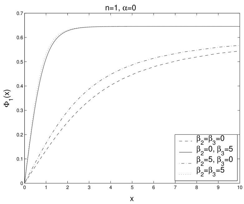
We were mainly interested in the effect of the potential. We thus first studied the behaviour of the Higgs field function $\Phi_{1}$ for different values of the coupling constants $\beta_{2}$ and $\beta_{3}$. Our results for the $n=1$ monopole are shown in Fig. 1. For $\beta_{2}=\beta_{3}=0$, $\Phi_{1}$ is given (analytically) by (21a). For $\beta_{2}=5$, $\beta_{3}=0$, the function still seems to decay power-law like rather than exponentially, while for both $\beta_{2}=0$, $\beta_{3}=5$ and $\beta_{2}=\beta_{3}=5$ the exponential decay is apparent. From (7), we see that for $\beta_{3}=0$ only one of the Higgs fields is massive, while all others remain massless. This can also be seen by an asymptotic analysis for the case $\beta_{3}=0$. We set

$$\Phi_{\gamma}=C_{\gamma}+\eta_{\gamma}\ ,\ \gamma=1,3,4\ \ \ {\rm with}\ \ \ C_{\gamma}=(\frac{\sqrt{5/3}}{2},\frac{\sqrt{5}}{3},\frac{1}{6})\ .$$ (22)

The linearised equations for the three Higgs field functions $\Phi_{1}$, $\Phi_{3}$ and $\Phi_{4}$ read (with the prime denoting the derivative with respect to $x$):

$$(x^{2}\eta_{\gamma}^{{}^{\prime}})^{{}^{\prime}}=x^{2}M_{\gamma\delta}\eta_{\delta}\ \ \ {\rm with}\ \ \ M_{\gamma\delta}=2C_{\gamma}C_{\delta}\ .$$ (23)

The matrix $M_{\gamma\delta}$ has one eigenvector, $C_{\gamma}$ itself with eigenvalue $2$ and two eigenvectors $C_{\delta_{1}}$, $C_{\delta_{2}}$, the ones orthogonal to $C_{\gamma}$, with eigenvalues $0$. The solution of the linearised equation is then given by:

$$\eta_{\gamma}=C_{\gamma}e^{-\sqrt{2}x}+c_{1}C_{\delta_{1}}/x+c_{2}C_{\delta_{2}}/x\ ,\ \ c_{1},c_{2}\ \ {\rm constant}$$ (24)

Clearly at large $x$, the power-law decay dominates the behaviour of the Higgs field functions.

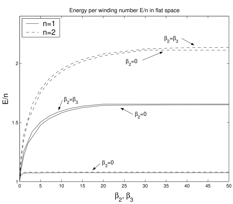
In Fig. 2 we present the mass per winding number of the $n=1$ monopole and the $n=2$ multimonopole in units of $4\pi\frac{\eta}{e}C$, $C=\frac{1}{2}\sqrt{\frac{5}{3}}$ for three different cases: a) $\beta_{2}\neq 0$, $\beta_{3}=0$, b) $\beta_{3}\neq 0$, $\beta_{2}=0$ and c) $\beta_{2}=\beta_{3}\neq 0$. Apparently, for all cases, the monopoles are in a repulsive phase, as expected. However, it seems that the mass depends only slightly on $\beta_{2}$. In the case of $\beta_{3}=0$, the potential can be written as a perfect square and thus resembles the potential of the SU(2) case. However, it should be noted that the present model is not an embedding in the sense that the vacuum expectation value has only two non-vanishing diagonal entries. We find the following values for the energy per winding number $E/n$ for the $n=1$ monopole and the $n=2$ multimonopole for $\beta_{2}$ (respectively $\beta_{3}$) $\rightarrow\infty$:

Table 1

	$n=1$	$n=2$
$\beta_{2}\rightarrow\infty$, $\beta_{3}=0$	$1.076$	$1.081$
$\beta_{3}\rightarrow\infty$, $\beta_{2}=0$	$1.650$	$2.112$
$\beta_{2}=\beta_{3}\rightarrow\infty$	$1.657$	$2.135$

These can be compared to the ones computed in the SU(2) case, where the mass per winding number has been obtained for $\tilde{\lambda}\rightarrow\infty$, where $\tilde{\lambda}$ is the Higgs self-coupling constant of the standard SU(2) Higgs potential $\tilde{V}=\frac{\tilde{\lambda}}{4}(\tilde{\Phi}^{2}-\tilde{\eta})^{2}$ . It was found that $E/n(\tilde{\lambda}\rightarrow\infty)$ is equal to $1.787$ for $n=1$ and equal to $2.293$ for $n=2$ [22, 11]. Comparing this, we see that the order of magnitude agrees with our results.

IV Gravitating solutions

A Spherically symmetric solutions

In the case of spherical symmetry ($n=1$), the gauge field functions $H_{1}$, $H_{3}$ and the Higgs field function $\Phi_{2}$ are identically zero. In addition $m=l$, $H_{2}=H_{4}$ and all functions depend only on $x$. We here give the explicit form of the equations to demonstrate the changes in comparison to the SU(2) case. For the axially symmetric case, these changes are analog. The equations for the remaining functions read (renaming $H_{2}=H_{4}\equiv K$ and the prime denoting the derivative with respect to $x$):

$$\frac{f^{{}^{\prime\prime}}}{f}+2\frac{f^{{}^{\prime}}}{fx}+\frac{1}{2}\frac{f^{{}^{\prime}}l^{{}^{\prime}}}{fl}-\frac{(f^{{}^{\prime}})^{2}}{f^{2}}=2\alpha^{2}\left(\frac{l}{f}U(\Phi_{1},\Phi_{3},\Phi_{4})+\frac{f}{lx^{4}}(K^{2}-1)^{2}+2\frac{f}{lx^{2}}(K^{{}^{\prime}})^{2}\right)$$ (25)

$$\frac{1}{2}\frac{l^{{}^{\prime\prime}}}{l}+\frac{3}{2}\frac{l^{{}^{\prime}}}{lx}-\frac{1}{4}\frac{(l^{{}^{\prime}})^{2}}{l^{2}}=2\alpha^{2}\left(\frac{l}{f}U(\Phi_{1},\Phi_{3},\Phi_{4})+\frac{f}{lx^{2}}(K^{{}^{\prime}})^{2}-\frac{K^{2}\Phi_{1}^{2}}{x^{2}}\right)$$ (26)

with

$$U(\Phi_{1},\Phi_{3},\Phi_{4})=-\frac{\beta_{2}^{2}}{2}\left(\Phi_{1}^{2}+\Phi_{3}^{2}+\Phi_{4}^{2}-1\right)^{2}$$ (27)

$$- \beta_{3}^{2}\left(\Phi_{1}^{2}(\frac{\Phi_{1}^{2}}{4}+\frac{9}{10}\Phi_{4}^{2}-\frac{7}{30})+\Phi_{3}^{2}(\frac{\Phi_{3}^{2}}{4}+\frac{2}{5}\Phi_{4}^{2}-\frac{7}{30}-\frac{4\sqrt{5}}{30}\Phi_{3}\Phi_{4})+\frac{7}{60}(\Phi_{4}^{2}-1)^{2}\right)$$ (28)

for the metric functions $f$ and $l$ and

$$\left(\frac{f}{\sqrt{l}}K^{{}^{\prime}}\right)^{{}^{\prime}}=\frac{f}{\sqrt{l}}K\left(\frac{K^{2}-1}{x^{2}}+\Phi_{1}^{2}\frac{l}{f}\right)$$ (29)

$$\left(x^{2}\sqrt{l}\Phi_{1}^{{}^{\prime}}\right)^{{}^{\prime}}=\frac{l^{3/2}x^{2}\Phi_{1}}{f}\left[\beta_{2}^{2}\left(\Phi_{1}^{2}+\Phi_{3}^{2}+\Phi_{4}^{2}-1\right)+\beta_{3}^{2}\left(\frac{\Phi_{1}^{2}}{2}+\frac{27}{30}\Phi_{4}^{2}-\frac{7}{30}\right)\right]+2K^{2}\sqrt{l}\Phi_{1}$$ (30)

$$\left(x^{2}\sqrt{l}\Phi_{3}^{{}^{\prime}}\right)^{{}^{\prime}}=\frac{l^{3/2}x^{2}\Phi_{3}}{f}\left[\beta_{2}^{2}\left(\Phi_{1}^{2}+\Phi_{3}^{2}+\Phi_{4}^{2}-1\right)+\beta_{3}^{2}\left(\frac{\Phi_{3}^{2}}{2}+\frac{2}{5}\Phi_{4}^{2}-\frac{1}{\sqrt{5}}\Phi_{3}\Phi_{4}-\frac{7}{30}\right)\right]$$ (31)

$$\left(x^{2}\sqrt{l}\Phi_{4}^{{}^{\prime}}\right)^{{}^{\prime}} = \frac{l^{3/2}x^{2}\Phi_{4}}{f}\left[\beta_{2}^{2}\left(\Phi_{1}^{2}+\Phi_{3}^{2}+\Phi_{4}^{2}-1\right)\right.$$ (32)

$$+ \left.\beta_{3}^{2}\left(-\frac{\Phi_{3}^{3}}{3\sqrt{5}\Phi_{4}}+\frac{9}{10}\Phi_{1}^{2}+\frac{2}{5}\Phi_{3}^{2}+\frac{7}{30}(\Phi_{4}^{3}-1)\right)\right]$$ (33)

for the gauge field function $K$ and the three Higgs field functions $\Phi_{i}$, $i=1,3,4$. In the case of gravitating solutions, i.e. $\alpha>0$, the solutions in the limit of $\beta_{2}=\beta_{3}=0$ have constant functions $\Phi_{3}$ and $\Phi_{4}$. We thus obtain for the mass exactly that obtained for the SU(2) monopoles [24] when we express it in units of $\frac{1}{2}\sqrt{\frac{5}{3}}$. Note, though, that in order to be able to compare the results obtained, we have to rescale $\alpha\rightarrow\frac{\alpha}{2}\sqrt{\frac{5}{3}}$.

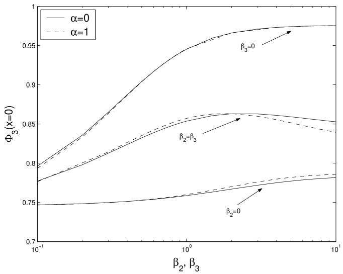
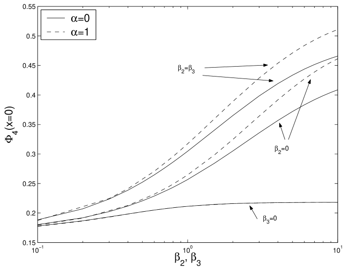
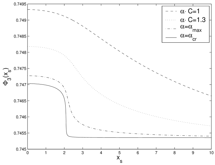
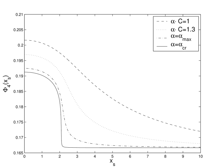
In order to demonstrate the influence of the Higgs coupling constants $\beta_{2}$, $\beta_{3}$, we show in Fig.s 3a and 3b the value of the Higgs field function $\Phi_{3}$ and $\Phi_{4}$, respectively, at the origin in dependence on the parameters $\beta_{2}$, $\beta_{3}$ for $\alpha=1$. For comparison, the corresponding values in flat space ($\alpha=0$) are also shown. Since in the BPS limit ($\beta_{2}=\beta_{3}=0$), the functions $\Phi_{3}$ and $\Phi_{4}$ are constant, all curves meet at $\frac{\sqrt{5}}{3}$ for $\Phi_{3}$ and $\frac{1}{6}$ for $\Phi_{4}$, respectively, in this limit. Again, it is apparent from these two figures that the parameter $\beta_{2}$ does not have a large influence. The functions $\Phi_{3}$ and $\Phi_{4}$ become monotonically decreasing functions of $x$ for the choices of $\beta_{2}$, $\beta_{3}$ shown in Fig.s 3a, 3b starting at the value shown with zero derivative and decreasing to their asymptotic values. The inclusion of gravity leads to an increase of $\Phi_{4}$ at $x=0$, while the value $\Phi_{3}(x=0)$ seems to depend only slightly on the parameter $\alpha$.

In order to be able to study further details of the $n=1$ solutions and be able to compare them with the SU(2) case, we have adopted the Schwarzschild-like ansatz for the metric used in [24, 25] rather than the isotropic ansatz (15):

$$ds^{2}=-A^{2}(r_{s})N(r_{s})dt^{2}+N^{-1}(r_{s})dr_{s}^{2}+r_{s}^{2}(d\theta^{2}+\sin^{2}\theta d\varphi^{2})\ .$$ (34)

The isotropic coordinate $r$ is relate to the Schwarzschild-coordinate $r_{s}$ through the following transformation [23]:

$$\frac{dr}{dr_{s}}=\frac{1}{\sqrt{N(r_{s})}}\frac{r}{r_{s}}$$ (35)

and thus can - for generic cases - only be obtained numerically.

In the SU(2) case, it was observed that the gravitating monopole solutions exist only up to a maximal value of the gravitational coupling $\tilde{\alpha}$, $\tilde{\alpha}_{max}$ [24]. $\tilde{\alpha}_{max}$ is a decreasing function of the Higgs self-coupling constant starting from $\tilde{\alpha}_{max}=1.403$ in the BPS limit. For bigger $\tilde{\alpha}$, the Schwarzschild radius becomes larger than the radius of the monopole core. Consequently, an extremal horizon $\tilde{x}_{h_{s}}$ forms with $N(\tilde{x}_{h_{s}})=\partial_{\tilde{x}}N|_{\tilde{x}=\tilde{x}_{h_{s}}}=0$ and in the limit $\tilde{\alpha}\rightarrow\tilde{\alpha}_{max}$ the solutions bifurcate with the branch of extremal Reissner-Nordström solutions. The solutions outside the horizon $\tilde{x}_{h_{s}}$ are described by this solutions, while in the interval $0\leq\tilde{x}\leq\tilde{x}_{h_{s}}$ they are non-trivial and non-singular. For small Higgs self-coupling a second branch of solutions was found extending backwards from $\tilde{\alpha}_{max}$ to $\tilde{\alpha}_{cr}<\tilde{\alpha}_{max}$ with $\tilde{\alpha}_{cr}=1.386$ in the BPS limit. The solutions then reach their limiting solution for $\tilde{\alpha}\rightarrow\tilde{\alpha}_{cr}$. For intermediate Higgs masses, a new phenomenon was observed [25]. A second, inner minimum appears that drops down much quicker to zero than the outer one. The limiting solution thus represents a non-abelian black hole. In the table below, we give $\alpha_{max}$, $\alpha_{cr}$ for $\beta_{2}=0$ in units of $\frac{1}{2}\sqrt{\frac{5}{3}}$ in order to be able to compare it with the SU(2) results. We also give the value of the outer minimum $N^{o}_{min}$ at the appearance of the second, inner minimum, if this phenomenon is observed.

Table 2

$\beta_{3}$	$\frac{1}{2}\sqrt{\frac{5}{3}}\cdot\alpha_{max}$	$\frac{1}{2}\sqrt{\frac{5}{3}}\cdot\alpha_{cr}$	$N^{o}_{min}$
$0$	$1.403$	$1.386$	$-$
$0.2$	$1.370$	$1.366$	$-$
$0.3$	$1.350$	$1.348$	$-$
$0.5$	$1.308$	$1.308$	$-$
$1$	$1.223$	$1.223$	$-$
$2$	$1.117$	$1.117$	$-$
$3$	$1.050$	$1.050$	$-$
$4$	$1.007$	$1.007$	$-$
$5$	$0.974$	$0.974$	$-$
$7$	$0.926$	$0.926$	$-$
$10$	$0.884$	$0.884$	$-$
$15$	$0.534$	$0.534$	$0.24\cdot 10^{-9}$
$16$	$0.851$	$0.851$	$0.49\cdot 10^{-7}$
$17$	$0.845$	$0.845$	$0.94\cdot 10^{-6}$
$20$	$0.829$	$0.829$	$0.37\cdot 10^{-4}$
$50$	$0.769$	$0.769$	$0.80\cdot 10^{-2}$
$100$	$0.746$	$0.746$	$0.21\cdot 10^{-1}$

Clearly, the phenomenon observed for intermediate Higgs masses in the SU(2) model [25] is observed here for $\beta_{3}\geq 15$, while a second branch of solutions exists only for $\beta_{3}\leq 0.3$. For all other $\beta_{3}$ we find that $\alpha_{max}=\alpha_{cr}$.

Analogous to the SU(2) case, the gravitating monopoles bifurcate with the branch of extremal Reissner-Nordström (RN) solutions in the limit $\alpha\rightarrow\alpha_{max}$ (resp. $\alpha\rightarrow\alpha_{cr}$). The approach to criticality is shown for the two Higgs fields $\Phi_{3}$, $\Phi_{4}$ in Fig.s 4a, 4b. for $\beta_{2}=0$, $\beta_{3}=0.3$. $\Phi_{3}$ and $\Phi_{4}$ are shown as functions of the dimensionless Schwarzschild-coordinate $x_{s}=e\eta r_{s}$ for four different values of the gravitational coupling $\alpha$. Clearly, the limiting solution is not yet reached for $\alpha_{max}$, but rather for $\alpha_{cr}<\alpha_{max}$, the numerical values of which are given in Table 2. An extremal horizon $x_{h_{s}}$ forms and $\Phi_{3}$ as well as $\Phi_{4}$ are constant and equal to their asymptotic values for $x_{s}\geq x_{h_{s}}$, while they are non-trivial for $x$ $\epsilon$ $[0:x_{h_{s}}]$. This is very similar to what was observed previously in the SU(2) case for the remaining matter field functions. Striking is that the two functions look qualitatively very similar in their approach to criticality.

Looking at the results of flat space, we expect that a similar pattern exists for the case of $\beta_{2}=\beta_{3}\neq 0$, while for $\beta_{2}\neq 0$, $\beta_{3}=0$, we find that $\alpha_{max}$ depends only very little on $\beta_{2}$.

B Axially symmetric solutions

While in flat space SU(2) monopoles as well as SU(5) monopoles - as was demonstrated by us in this paper - are either repelling or non-interacting (in the BPS limit), it was shown in the SU(2) case [12] that gravity is able to overcome the repulsion for sufficiently small Higgs boson masses. We thus limit our analysis of axially symmetric SU(5) monopoles to this important point. We find that for a fixed $\alpha$ the values of $\beta^{eq}_{2}$, $\beta^{eq}_{3}$ for which the mass of the $n=1$ monopole is equal to the mass per winding number of the $n=2$ multimonopole roughly forms a half-circle in the $\beta_{2}$-$\beta_{3}$-plane. E.g. we find for $\alpha=1.4$, that for $\beta_{3}=0$ the value of $\beta^{eq}_{2}\approx 0.045$, while for $\beta_{2}=0$ we have $\beta^{eq}_{3}\approx 0.043$ and for $\beta^{eq}_{2}=\beta^{eq}_{3}\approx 0.03$. This suggests that

$$\sqrt{\beta^{eq}_{2}(\alpha)+\beta^{eq}_{3}(\alpha)}\approx C_{1}(\alpha)\ \ ,\ \ {\rm with}\ \ C_{1}\ \ {\rm constant}\ .$$ (36)

We find that $C_{1}$ is an increasing function of $\alpha$, e.g. we find that $C_{1}(\alpha=1.6)\approx 0.056$ and $C_{1}(\alpha=1.8)\approx 0.2$. This latter value of $C_{1}$ for $\alpha=1.8$ suggests in comparison with the other two that $C_{1}$ is in fact a strongly increasing function of $\alpha$. This is indeed what was also found in the SU(2) case [12]. Moreover, the order of magnitude of $\beta^{eq}_{2}$, $\beta^{eq}_{3}$ agrees with what was found in the SU(2) case. This thus suggests that also in the SU(5) case, bound multimonopoles only exist for sufficiently small values of the Higgs self-coupling constants.

V Non-abelian black holes

For the numerical construction of non-abelian black holes, we followed [23] and introduced new metric functions $f_{2}$, $l_{2}$ and $m_{2}$

$$f_{2}=\frac{f}{z^{2}}\ ,\ \ l_{2}=\frac{l}{z^{2}}\ ,\ \ m_{2}=\frac{m}{z^{2}}\ ,$$ (37)

where $z=1-\frac{x_{h}}{x}$ is the compactified coordinate that maps the infinite interval $[x_{h}:\infty[$ to the finite interval $[0:1]$. The new boundary conditions at the horizon $x_{h}$ now read [23]:

$$\left(f_{2}-\frac{\partial f_{2}}{\partial z}\right)|_{z=0}=0\ ,\ \ \left(m_{2}+\frac{\partial m_{2}}{\partial z}\right)|_{z=0}=0\ ,\ \ \left(l_{2}+\frac{\partial l_{2}}{\partial z}\right)|_{z=0}=0\ .$$ (38)

The isotropic horizon $x_{h}$ is not a physical quantity. We thus determine for every solution obtained the parameter $x_{\Delta}$ given by:

$$x_{\Delta}=\sqrt{\frac{A}{4\pi}}\ \ {\rm with}\ \ A=2\pi\int_{0}^{\pi}d\theta\sin\theta x_{h}^{2}\frac{\sqrt{l_{2}(x=x_{h},\theta)m_{2}(x=x_{h},\theta)}}{f_{2}(x=x_{h},\theta)}\ .$$ (39)

$A$ is the area of the horizon and directly related to the entropy $S$ of the black hole: $S=\frac{A}{4}$. Note that the Schwarzschild-like horizon $x_{h_{s}}$ is exactly defind to be the radius of the horizon with area $A$.

A Spherically symmetric solutions

Spherically symmetric black hole solutions can be constructed for $n=1$. Similarly as in the case of regular solutions they have $m_{2}=l_{2}$, $H_{2}=H_{4}$, $H_{1}$=$H_{3}$=$\Phi_{2}=0$ and all remaining functions depend only on $x$. In fact the non-abelian black hole solutions can equally well be constructed using the Ansatz of the Schwarschild-like metric. The boundary conditions are then directly imposed at $x=x_{h_{s}}=x_{\Delta}$.

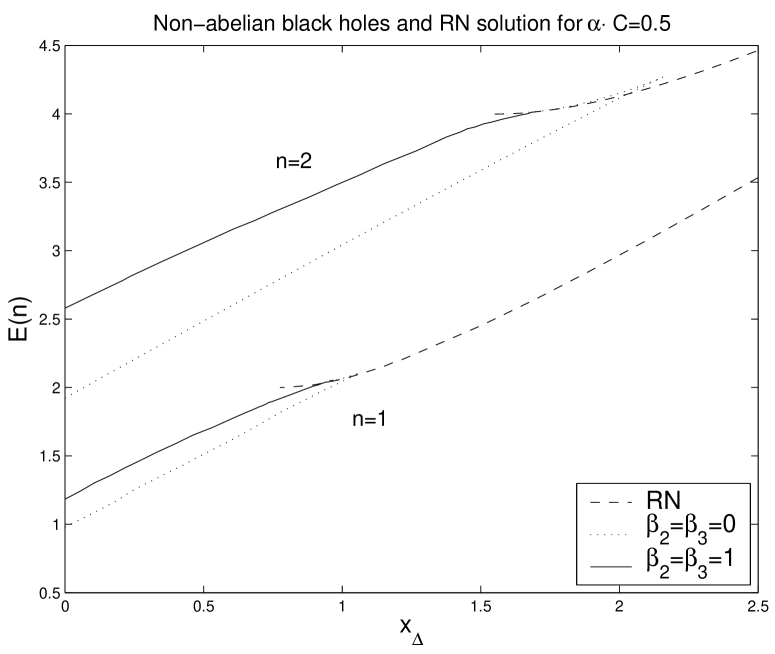
We find that the domain of existence of the spherically symmetric non-abelian black holes in the $\alpha$-$x_{\Delta}$-plane is of similar shape than the domain of existence in the SU(2) [24] and in the SU(3) [26] case, respectively. Fixing $\alpha$ and increasing $x_{\Delta}$, the non-abelian solutions exist for $x_{\Delta}\leq x_{\Delta}^{max}$ and at $x_{\Delta}=x_{\Delta}^{cr}$ bifurcate with the branch of non-extremal Reissner-Nordström (RN) solution for small $\alpha$ and with the branch of extremal Reissner-Nordström (RN) solution for large $\alpha$, respectively. In this paper, we put emphasis on the case $\alpha\cdot C=0.5$, $C=\frac{1}{2}\sqrt{\frac{5}{3}}$, for which the solutions bifurcate with the branch of non-extremal RN solutions. For $\beta_{2}=\beta_{3}=0$ the bifurcation occurs on a second branch of solutions which exists for $x_{\Delta}^{cr}\leq x_{\Delta}\leq x_{\Delta}^{max}$, i.e. that in this interval two different black hole solutions can be constructed. For $\beta_{2}=\beta_{3}$ sufficiently large only one branch of solutions exists and $x_{\Delta}^{max}=x_{\Delta}^{cr}$. This is demonstrated in Fig. 5 for $n=1$ and $\beta_{2}=\beta_{3}=0$, resp. $\beta_{2}=\beta_{3}=1$. We show the energy $E(1)$ of the non-abelian solutions and that of the corresponding RN solutions. The occurence of a second branch of solutions for $\beta_{2}=\beta_{3}=0$ is apparent from this figure with $x_{\Delta}^{max}\approx 1.064$ and $x_{\Delta}^{cr}\approx 0.936$. For $\beta_{2}=\beta_{3}=1$ only one branch of solutions exists and we find that $x_{\Delta}^{max}=x_{\Delta}^{cr}\approx 0.9676$.

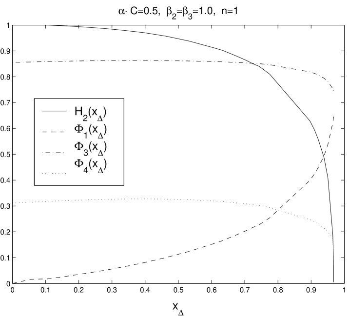
A good indication for the bifurcation with the branch of non-extremal RN solutions is the fact that in the limit $x_{\Delta}\rightarrow x_{\Delta}^{cr}$ the values of the matter fields at the horizon tend to their asymptotic values. Since these functions are monotonic functions of $x$, they obviously become constant on the whole interval $[x_{\Delta}:\infty[$ in the critical limit. We demonstrate this in Fig. 6 for $H_{2}(x_{\Delta})$ and $\Phi_{a}(x_{\Delta})$, $a=1,3,4$. The value of the gauge function at the horizon, $H_{2}(x_{\Delta})$, tends to zero, while the values of the three Higgs field function at the horizon, $\Phi_{a}(x_{\Delta})$, approach their respective asymptotic values (see (19c)).

B Axially symmetric solutions

In the SU(2) case, it was found [23] that the critical values of the horizon parameter $x_{\Delta}$ increase with increasing $n$. However, it was also shown that the qualitative shape of the domain of existence doesn’t change. We observe the same for the SU(5) case. This is demonstrated in Fig. 5, where we shown together with the energy of the $n=1$ solutions the energy $E(2)$ of the axially symmetric black hole solutions for two different values of $\beta_{2}=\beta_{3}$. Clearly, the solutions exist for higher values of $x_{\Delta}$. We find for $\beta_{2}=\beta_{3}=0$ that $x_{\Delta}^{max}\approx 2.158$ and $x_{\Delta}^{cr}\approx 1.667$, while for $\beta_{2}=\beta_{3}=1$, we have $x_{\Delta}^{max}=x_{\Delta}^{cr}\approx 1.691$. Indeed, this figure demonstrates again the occurence of a second branch of solutions for $\beta_{2}=\beta_{3}=0$, while for $\beta_{2}=\beta_{3}=1$ only one branch of non-abelian black hole solutions exists.

As an indication of the deformation of the horizon, which is defined to be the surface of constant $x_{h}$, we have computed the circumference of the horizon along the equator $L_{e}$

$$L_{e}=\int_{0}^{2\pi}d\varphi\sqrt{g_{\varphi\varphi}}\mid_{x=x_{h},\theta=\pi/2}=2\pi x_{h}\sqrt{\frac{l(x=x_{h},\theta=\pi/2)}{f(x=x_{h},\theta=\pi/2)}}$$ (40)

and the circumference of the horizon along the poles $L_{p}$:

$$L_{p}=2\int_{0}^{\pi}d\theta\sqrt{g_{\theta\theta}}\mid_{x=x_{h},\varphi=const.}=2x_{h}\int_{0}^{\pi}d\theta\sqrt{\frac{m(x=x_{h},\theta)}{f(x=x_{h},\theta)}}\ .$$ (41)

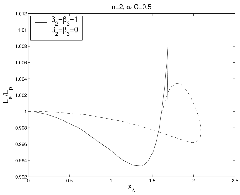
It is apparent that the ratio $L_{e}/L_{p}$ is equal to one for the spherically symmetric solutions since $l=m$ for $n=1$ and the angle dependence disappears. For the axially symmetric solutions, however, the ratio deviades from one. This is demonstrated in Fig. 7, where we show $L_{e}/L_{p}$ as function of $x_{\Delta}$ for the $n=2$ non-abelian black hole with $\alpha\cdot C=0.5$, $C=\frac{1}{2}\sqrt{\frac{5}{3}}$. The case $\beta_{2}=\beta_{3}$ is the analog of what was studied in the SU(2) case for $\tilde{\lambda}=0$. The ratio reaches a minimum at a value of $x_{\Delta}$ close to the maximal $x_{\Delta}$, then on the second branch of solutions reaches a maximal value which is bigger than one and then drops down to one at $x_{\Delta}=x^{cr}_{\Delta}$. For non-vanishing Higgs coupling constants (we have chosen $\beta_{2}=\beta_{3}=1$), the apparent effect is the decrease of the minimal and the increase of the maximal value of $L_{e}/L_{p}$. Thus the inclusion of the Higgs potential increases the deformation of the regular horizon of the non-abelian black holes. The qualitative feature changes in the sense that now no second branch of solutions exists and thus the local extrema of the curve are reached for $x_{\Delta}<x^{cr}_{\Delta}$. Moreover, we observe a sharp drop of the ratio from its maximal value to the value one at $x_{\Delta}=x^{cr}_{\Delta}$. Fig. 7 leads us further to the conclusion that the observation of two local extrema (a minimum and a maximum) for the ratio $L_{e}/L_{p}$ seems a generic feature for all Higgs coupling constants as long as the critical solutions into which the non-abelian black holes merge at $x_{\Delta}=x^{cr}_{\Delta}$ are non-extremal Reissner-Nordström solutions.

VI Summary and Conclusions

Since it is believed that monopoles have formed in the early universe through the spontaneous symmetry breakdown of a Grand Unified Theory (GUT) down to a gauge group containing a $U(1)$ subgroup, the study of monopoles arising in SU(5) Yang-Mills-Higgs theory which (through an appropriate potential) is spontaneously broken down to $SU(3)\times SU(2)\times U(1)$ seems of importance.

We have thus studied spherically as well as axially symmetric solutions in SU(5) Yang-Mills-Higgs theory both in flat and curved space. Concerning the globally regular solutions, we find that in flat space very similar to the corresponding solutions in SU(2) Yang-Mills-Higgs theory, the monopoles are either non-interacting or repelling. Moreover, we find that the order of magnitude of the mass in the limit of the Higgs self-coupling constants going to infinity agrees with the SU(2) results. Minimal coupling of gravity to the system leads in principle to two different types of non-abelian solutions: a) globally regular, gravitating monopoles and b) non-abelian black holes. We find that the qualitative features like the appearance of a second branch of solutions for small Higgs self-coupling constants or the appearance of a new phenomenon for intermediate values of the Higgs self-coupling constants are also found in this system. Since these phenomena have also been observed for spherically symmetric solutions in SU(3) Einstein-Yang-Mills-Higgs theory (EYMH) [26], it is likely that what was observed in SU(2) seems to be a generic feature of SU(N) EYMH theory with the Higgs field in the adjoint representation.

We also studied spherically and axially symmetric non-abelian black holes solutions. The corresponding solutions for the SU(2) gauge group were studied in great detail in [23] for vanishing Higgs coupling constant (BPS limit). It seems, however, that the “physically” relevant solutions related to SU(5) have to be constructed for non-vanishing values of the Higgs self-coupling constants $\beta_{2}$, $\beta_{3}$. That’s why we have put emphasis on the influence of a non-trivial Higgs potential on the solutions. Of course, the problem is numerically involved since the equations have to be solved for four continuous parameters: $\beta_{2}$, $\beta_{3}$, $\alpha$ and $x_{h}$. In addition there is a discrete parameter, namely the winding number $n$. Nevertheless, we have tried to determine the main features of the influence of the potential on the solutions. We find that: (i) the parameters $\beta_{2}$ and $\beta_{3}$ effect in a non negligible way the domain of existence in the $\alpha$-$x_{\Delta}$-plane, (ii) for $\beta_{2}$, $\beta_{3}$ large enough, the solutions bifurcate into a non-extremal Reissner-Nordström solution on the first branch of solutions without a backbending in the parameter $x_{\Delta}$, (iii) the deformation of the horizon of the axially symmetric black hole solutions increases for $\beta_{2}$, $\beta_{3}\neq 0$, (iv) the surface gravity - at least for small values of $\beta_{2}$, $\beta_{3}$ - depends only weakly on $\beta_{2}$, $\beta_{3}$.

Acknowledgements Y. B. is grateful to the Belgian F. N. R. S. for financial support. B. H. was supported by the EPSRC. We thank CERN for financial support and its hospitality.

FIG. 1.: The Higgs field function $\Phi_{1}(x)$ is shown as function of $x$ for $n=1$, $\alpha=0$ and four different choices of the coupling constants $\beta_{2}$, $\beta_{3}$.

FIG. 2.: The energy per winding number $E/n$ in units of $4\pi\frac{\eta}{e}C$, $C=\frac{1}{2}\sqrt{\frac{5}{3}}$ is shown for the $n=1$ monopole (solid) and the $n=2$ multimonopole (dashed) for $\beta_{3}=0$, respectively $\beta_{2}=0$, respectively $\beta_{2}=\beta_{3}$, as function of $\beta_{2}$, respectively $\beta_{3}$.

FIG. 3a.: The value of the Higgs field function $\Phi_{3}(x)$ at the origin, $\Phi_{3}(x=0)$, is shown for the $n=1$ monopole as function of $\beta_{2}$ ($\beta_{3}$, respectively) for $\alpha=0$ and $\alpha=1$, respectively.

FIG. 3b.: The value of the Higgs field function $\Phi_{4}(x)$ at the origin, $\Phi_{4}(x=0)$, is shown for the $n=1$ monopole as function of $\beta_{2}$ ($\beta_{3}$, respectively) for $\alpha=0$ and $\alpha=1$, respectively.

FIG. 4a.: The Higgs field function $\Phi_{3}(x_{s})$ is shown for the $n=1$ monopole as function of the dimensionless Schwarzschild coordinate $x_{s}=e\eta r_{s}$ for $\beta_{2}=0$, $\beta_{3}=0.3$ for four different values of $\alpha$ (with $C=\frac{1}{2}\sqrt{\frac{5}{3}}$) including $\alpha=\alpha_{cr}$.

FIG. 4b.: Same as Fig. 4a but for the Higgs field function $\Phi_{4}(x_{s})$.

FIG. 5.: The energy $E(n)$ in units of $4\pi\frac{\eta}{e}C$, $C=\frac{1}{2}\sqrt{\frac{5}{3}}$ is shown for the $n=1$ and the $n=2$ non-abelian black hole as function of $x_{\Delta}$ for two values of $\beta_{2}=\beta_{3}$ and $\alpha\cdot C=0.5$. For comparison, also the energy of the corresponding Reissner-Nordström (RN) solution is shown.

FIG. 6.: The values of the gauge field function $H_{2}$ and the three Higgs field functions $\Phi_{1}$, $\Phi_{3}$ and $\Phi_{4}$ at the horizon $x_{\Delta}$ of the spherically symmetric $n=1$ non-abelian black hole are shown as function of $x_{\Delta}$ for the $\alpha\cdot C=0.5$, $C=\frac{1}{2}\sqrt{\frac{5}{3}}$, and $\beta_{2}=\beta_{3}=1$.

FIG. 7.: The ratio of the circumference of the horizon along the equator $L_{e}$ and the circumference of the horizon along the poles $L_{p}$ is shown as function of $x_{\Delta}$ for the axially symmetric $n=2$ non-abelian black holes for two values of $\beta_{2}=\beta_{3}$ and $\alpha\cdot C=0.5$, $C=\frac{1}{2}\sqrt{\frac{5}{3}}$.

REFERENCES

- [1] H. Georgi and S. Glashow, Phys. Rev. Lett. 32 (1974), 438.
- [2] E. Kolb and M. Turner, Addison Wesley, 1993.
- [3] see eg : K. Hirata et al., Phys. Lett. B220 (1989), 308; R. Becker-Szendy et al., Phys. Rev. D42 (1990), 2974; M. Shiozawa et al., Phys. Rev. Lett. 81 (1998), 3319.
- [4] G. ’t Hooft, Nucl. Phys. B79 (1974), 276; A. Polyakov, JETP Lett. 20 (1974), 194.
- [5] B. Bogomol’nyi, Sov. J. Nucl. Phys. 24 (1976), 449.
- [6] see e.g. A. Jaffe and C. Taubes, Vortices and monopoles, Birkhäuser, 1980.
- [7] C. Rebbi and P. Rossi, Phys. Rev. D22 (1980), 2010; R. Ward, Commun. Math. Phys. 79 (1981), 317; P. Forgacs, Z. Horvath and L. Palla, Phys. Lett. B99 (1981), 232; E. Corrigan and P. Goddard, Commun. Math. Phys. 80 (1981), 575; M. Prasad, Commun. Math. Phys. 80 (1981), 137; M. K. Prasad and P. Rossi, Phys. Rev. D 24 (1981), 2182.n
- [8] M. Prasad and C. Sommerfield, Phys. Rev. Lett. 35 (1975), 159.
- [9] N. Manton, Nucl. Phys. B126 (1977), 525; J. Goldberg, P. Yang, S. Park and K. Wali, Phys. Rev. D18 (1978), 542; W. Nahm, Phys. Lett. B79 (1978), 426; Phys. Lett. B85 (1979), 373.
- [10] L. O’Raifeartaigh, S. Y. Yark and K. C. Wali, Phys. Rev. D20 (1979), 1941.
- [11] B. Kleihaus, J. Kunz and D. H. Tchrakian, Mod. Phys. Lett. A13 (1998), 2523.
- [12] B. Hartmann, B. Kleihaus and J. Kunz, Phys. Rev. Lett. 86 (2001), 1422; Phys. Rev. D65 (2002), 0240027.
- [13] Y. Brihaye and B. Hartmann, Phys. Lett. B528 (2002), 288; Phys. Lett. B534 (2002), 137; B. Hartmann, Phys. Lett. B541 (2002), 368.
- [14] E. Corrigan, D. Olive, D. Fairlie and J. Nuyts, Nucl. Phys. B106 (1976), 475; T. Dereli and L. Swank, COO-3075-137 Yale print, (1976).
- [15] Y. Brihaye and J. Nuyts, J. Math. Phys. 18 (1977), 2177.
- [16] C. P. Dokos and T. N. Tomaras, Phys. Rev. D21 (1980), 2940; D. Scott, Nucl. Phys. B171 (1980), 95.
- [17] E. Weinberg, Nucl. Phys. B167 (1980), 500.
- [18] It should be mentioned here, though, that in a recent paper (H. Adarkar, S. Dugad, M. Krishnaswamy, M. Menon and B. Sreekantan, hep-ex/0008074) results have been presented that suggest the lifetime of the proton to be roughly , which would fit nicely with an SU(5) GUT.
- [19] T. Vachaspati, Phys. Rev. Lett. 76 (1996), 188; H. Liu, T. Vachaspati, Phys. Rev. D56 (1997), 1300.
- [20] M. Meckes, hep-th/0202001
- [21] L. Pogosian and T. Vachaspati, Phys. Rev. D62 (2000), 105005.
- [22] E. B. Bogomol’nyi and M. S. Marinov, Sov. J. Nucl. Phys. 23 (1976), 357.
- [23] B. Hartmann, B. Kleihaus and J. Kunz, Phys. Rev. D65 (2002), 024027.
- [24] P. van Nieuwenhuizen, D. Wilkinson and M. Perry, Phys. Rev. 13 (1976), 778; K. Lee, V. P. Nair and E. J. Weinberg, Phys. Rev. D45 (1992), 2751; P. Breitenlohner, P. Forgacs, D. Maison, Nucl. Phys. B383 (1992), 357; Nucl. Phys. B442 (1995), 126; P. C. Aichelburg and P. Bizon, Phys. Rev. D48 (1993), 607.
- [25] A. Lue and E. J. Weinberg, Phys. Rev. D60 (1999), 084025; Y. Brihaye, B. Hartmann and J. Kunz, Phys. Rev. D62 (2000), 044008.
- [26] Y. Brihaye and B. Piette, Phys. Rev. D64 (2001), 084010.