Experimental String Field Theory

Davide Gaiotto and Leonardo Rastelli

Physics Department, Princeton University, Princeton, NJ 08544

E-mail: dgaiotto, lrastell@princeton.edu

Abstract

We develop efficient algorithms for level-truncation computations in open bosonic string field theory. We determine the classical action in the universal subspace to level (18,54) and apply this knowledge to numerical evaluations of the tachyon condensate string field. We obtain two main sets of results. First, we directly compute the solutions up to level $L=18$ by extremizing the level-truncated action. Second, we obtain predictions for the solutions for $L>18$ from an extrapolation to higher levels of the functional form of the tachyon effective action. We find that the energy of the stable vacuum overshoots -1 (in units of the brane tension) at $L=14$, reaches a minimum $E_{min}=-1.00063$ at $L\sim 28$ and approaches with spectacular accuracy the predicted answer of -1 as $L\to\infty$. Our data are entirely consistent with the recent perturbative analysis of Taylor and strongly support the idea that level-truncation is a convergent approximation scheme. We also check systematically that our numerical solution, which obeys the Siegel gauge condition, actually satisfies the full gauge-invariant equations of motion. Finally we investigate the presence of analytic patterns in the coefficients of the tachyon string field, which we are able to reliably estimate in the $L\to\infty$ limit.

1 Introduction and Summary

The realization that D-branes are solitons of the open string tachyon [1, 2] has triggered a revival of interest in open string field theory. Much work has focused on the search for classical solutions of cubic bosonic open string field theory [3] (OSFT). Despite important technical progress in the understanding of the open string star product - notably the discovery of star algebra projectors [4, 5] and of new connections with non-commutative field theory [6, 7, 8, 9] - analytic classical solutions of OSFT are still missing.

Fortunately, the OSFT equations of motion can be solved numerically in the ‘level-truncation’ scheme invented by Kostelecky and Samuel [17]. The open string field is restricted to modes with an $L_{0}$ eigenvalue smaller than a prescribed maximum ‘level’ $L$. For any finite $L$, the truncated OSFT action contains a finite number of fields and numerical computations are possible. Remarkably, numerical results [17]-[37] for various classical solutions appear to converge rapidly to the expected answers as the level $L$ is increased. Much of our present intuition about the classical dynamics of OSFT comes from the level truncation scheme, and in fact even in vacuum string field theory [10, 11] several exact results were first guessed based on numerical data.

This motivated us to develop efficient algorithms for level-truncation calculations. Our main technical innovations are the systematic use of conservation laws [4] to compute the cubic vertices, and the implementation of our algorithms on a C++ code. In this paper we apply these methods to the evaluation of the classical action in the universal subspace [2, 4], which is the space of string fields generated by ghost oscillators and matter Virasoro generators acting on the vacuum. Using conservation laws we determine the classical action directly in the universal basis in a recursive way, with an algorithm whose complexity is linear in the number of vertices (cubic in the number of fields). Some details about the numerical algorithms can be found in appendix A of the paper. The gain in efficiency of our methods is of several orders of magnitude, and we are able to obtain the $10^{10}$ universal cubic vertices at level (18,54).

The universal subspace has special physical significance because it contains the tachyon condensate string field, the solution of OSFT corresponding to the stable vacuum of the open string tachyon. Its (negative) energy per unit volume must exactly cancel the D-brane tension. Sen and Zwiebach’s computation [18] of the tachyon condensate up to level (4,8) gave the first evidence that OSFT reproduces the correct D-brane physics. Moeller and Taylor [20] pushed the computation to level (10,20) finding that 99.91% of the D-brane tension is cancelled in the tachyon vacuum. Given such a remarkable agreement, it may appear quite pointless to extend their results to higher level. Not so. Up to level 10, the individual coefficients of the string field appear to converge much less rapidly than the value of the action. A more precise determination of the coefficients is likely to provide clues for an exact solution. Indeed various surprising patterns obeyed by OSFT solutions were ‘experimentally’ observed in [37], but more accurate results are needed to decide which of these patterns are likely to be exact and which ones only approximate. Higher level computations can also be expected to shed light on the nature of the level truncation procedure itself, which still lacks a sound theoretical justification.

Our first main set of results (described in section 3) is the computation of the Siegel gauge tachyon condensate in level-truncation up to $L=18$. The procedure is the standard one: at any given level $L$, there are $N_{L}$ scalar fields that obey the Siegel condition, and we determine their vev’s by solving the $N_{L}$ equations of motion implied by the gauge-fixed action. There is a potential subtlety here: the full equations of motion before gauge-fixing impose a bigger number of constraints [29] (the extra conditions simply enforce extremality of the action along gauge orbits). Consistency demands that the full set of equations of motion is satisfied as $L\to\infty$, and we systematically check that this indeed happens, with remarkable accuracy. As another consistency check, we verify that the tachyon condensate obeys the quadratic relations analytically derived by Schnabl [38], and we again find excellent agreement.

$L$	$E_{(L,3L)}$	$E_{(L,2L)}$
2	-0.9593766	-0.9485534
4	-0.9878218	-0.9864034
6	-0.9951771	-0.9947727
8	-0.9979302	-0.9977795
10	-0.9991825	-0.9991161
12	-0.9998223	-0.9997907
14	-1.0001737	-1.0001580
16	-1.0003754	-1.0003678
18	-1.0004937	-1.00049

Table 1: Values of the vacuum energy in level-truncation, in the $(L,3L)$ and $(L,2L)$ approximation schemes.

The values of the vacuum energy as a function of $L$ are shown in Table 1. Unexpectedly, at $L=14$ the energy overshoots the predicted answer of -1 and appears to further decrease at higher levels. As a first reaction, one may wonder whether the level-truncation procedure is breaking down for $L>10$, as could happen if the approximation was only asymptotic. In this pessimistic scenario, for any OSFT observable there would be a maximum level that gives the estimate closest to the ‘exact’ value, and beyond this optimal level the procedure would stop converging. However, the data favor a smooth behavior as $L$ increases, since the differences between consecutive approximations are getting smaller.

The results in Table 1 may simply indicate that the approach of the energy to -1 as $L\to\infty$ is non-monotonic, contrary to previous naive expectations. Indeed, Taylor has recently presented convincing evidence [39] for this benign interpretation of our results. He applies a clever extrapolation technique to level-truncation data for $L\leq 10$ to estimate the vacuum energies even for $L>10$. This procedure reproduces quite accurately our exact values in Table 1 and further predicts that the vacuum energy reaches a minimum for $L\sim 28$, but then turns back to approach asymptotically -1 for $L\to\infty$.

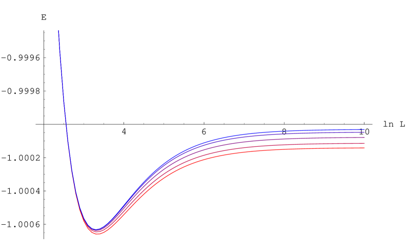
Figure 1: Curves of the vacuum energy as a function of level, as predicted by our extrapolation scheme for various values of $M$ (maximum level of the data used in the extrapolation). The figure shows the curves $E^{(M)}(L)$ on a logarithmic plot, for $M$ between 8 (lowermost curve) and 16 (uppermost curve). Data in the $(L,3L)$ scheme.

In sections 4 we introduce our second main set of results. We devise an extrapolation technique in the same spirit of Taylor’s analysis. We consider the effective tachyon potential $V_{L}(T)$ around the unstable vacuum, obtained by classically integrating out all the higher scalars up to level $L$. $V_{L}(T)$ is computed ‘non-perturbatively’ by fixing the value of $T$ and solving numerically the equations of motion for the other scalars. We are able to obtain $V_{L}(T)$ up to $L=16$. Clearly for each $L$, the minimum of $V_{L}(T)$ is just the vacuum energy $E_{L}$ at level $L$. However the functional dependence on $T$ contains more information than just the extremal value $E_{L}$. The idea is to perform an extrapolation in $L$ of the whole functions in $T$. In practice, we consider a finite interval of values of $T$ around the non-perturbative minimum. For a fixed $T$ in this interval we interpolate our data for $V_{L}(T)$ with a polynomial in $1/L$, and then extrapolate this polynomial to higher levels. To check the stability of this approximation scheme, we vary the maximum level $M$ of the set of data used as input for the extrapolation: for each $M\leq 16$, we apply the extrapolation to the functions $\{V_{L}(T)\,|\,L\leq M\}$. This gives estimates $T_{L}^{(M)}$ for the tachyon vev and for the corresponding vacuum energy $E^{(M)}_{L}$, for any $L>M$.

	$L_{min}$	$E_{min}$	$E_{\infty}$
$M=6$	41.1	-1.001171	-1.000949
$M=8$	28.2	-1.000660	-1.000140
$M=10$	27.8	-1.000646	-1.000113
$M=12$	27.5	-1.000637	-1.000077
$M=14$	27.3	-1.000633	-1.000046
$M=16$	27.3	-1.000632	-1.000030

Table 2: Parameters of the curves $E^{(M)}(L)$ (in the $(L,3L)$ scheme). The energy reaches its minimum $E_{min}$ for $L=L_{min}$, and tends asymptotically to $E_{\infty}$ as $L\to\infty$.

The predicted power of the method is quite impressive. For example, with $M=10$, that is using only level-truncation results up to level 10, the estimate $T^{(10)}_{18}$ reproduces with an accuracy of $10^{-5}$ the exact tachyon vev $T_{18}$, obtained by straightforward level-truncation at $L=18$. This is remarkable, since the former computation is over a thousand times faster than the latter.

Figure 1 and Table 2 summarize the extrapolations of the energy as a function of level, for various values of $M$. The data completely confirm (with enhanced precision) the conclusions of Taylor [39]. The behavior of the energy as a function of level is non-monotonic, but eventually the asymptotic limit of -1 is reached with spectacular accuracy.

These results greatly reassure us of the validity of the level-truncation scheme. Observables in OSFT have a smooth limit as $L\to\infty$, which (in the absence of an alternative definition) should be identified with their ‘exact’ value. In all cases where an independent prediction for the observable is available (as for the vacuum energy, or for Schnabl’s quadratic identities), the $L\to\infty$ extrapolation gives the correct answer.

A practical lesson of this analysis is that polynomial interpolations in $1/L$ have great predictive power, at least for the $(L,3L)$ approximation scheme. This observation makes the level-truncation scheme much more efficient, as reliable estimates can be extracted from (relatively) painless numerical work.

In section 5 we describe the results for the individual coefficients of the tachyon string field extrapolated to $L=\infty$. The main conclusions are:

• The asymptotic value of the tachyon vev is $T_{\infty}\simeq 0.5405$, ruling out the conjecture [29] for an exact value $T_{HS}=\sqrt{3}/\pi\cong 0.5513$.

• The conjectured universality [37] of certain ghost coefficients seems to be somewhat problematic in view of our data. While most coefficients come strikingly close to the conjectured values, the coefficient of $c_{-1}|0\rangle$ deviates by $2\%$ from the expected answer. Our predictions for the $L=\infty$ string field are likely to have a smaller error.

• The ‘quasi-pattern’ observed in [37] of an approximate factorization of $L_{0}{\cal T}_{Siegel}$, where ${\cal T}_{Siegel}$ is the Siegel-gauge tachyon condensate, gets worse in our $L=\infty$ extrapolations. So this is definitely not an exact property.

• The correspondence between OSFT equations of motion in Siegel gauge and a certain equation for ghost number zero string fields [37] is still rather well obeyed, but does not improve in the $L=\infty$ extrapolations. This is likely an approximate pattern, as already suspected in [37].

We hope that our accurate data will stimulate new imaginative approaches to the problem of finding an exact solution. In the near future it will be possible to extract from our results new information about the kinetic term around the tachyon vacuum. It will also be straightforward to extend the methods of this paper to the computation of more general classical solutions of OSFT, which should provide more analytic clues.

A more complete set of numerical data that it is practical to reproduce here (coefficients at higher levels, more significant figures etc.) will be be made available on-line [40].

To make this paper self-contained, we begin in the next section with a review of some basics.

2 OSFT and the Universal Tachyon Condensate

In this section we describe the basic setup for classical equations of motion in OSFT, with an emphasis on the symmetries obeyed by the tachyon condensate string field in Siegel gauge. While none of the results presented in this section are really new, we take the opportunity to spell out some facts - in particular our summary equation (2.1.3) - that are not widely known.

2.1 The Tachyon Condensate

The action of OSFT takes the well-known (deceptively) simple form [3]

$$S=-\frac{1}{g^{2}}\left(\frac{1}{2}\langle\Psi,Q_{B}\Psi\rangle+\frac{1}{3}\,\langle\Psi,\Psi*\Psi\rangle\right)\,.$$ (2.1)

This action describes the worldvolume dynamics of a D-brane specified by some Boundary CFT. The string field $\Psi$ belongs to the full matter+ghost state-space of this BCFT. In classical OSFT, $\Psi$ has ghost number one. According to Sen’s conjecture [1], the classical OSFT eom’s

$$Q_{B}\Psi+\Psi*\Psi=0\,$$ (2.2)

must admit a Poincaré invariant solution $\Psi\equiv{\cal T}$ corresponding to the condensation of the open string tachyon to the vacuum with no D-branes. The tachyon potential ${\cal{V}}(\Psi)$ is given by [2]

$${{\cal V}(\Psi)\over 2\pi^{2}M}\equiv\frac{1}{2\pi^{2}}f(\Psi)=\,{1\over 2}\langle\Psi,Q_{B}\Psi\rangle+{1\over 3}\,\langle\,\Psi,\Psi*\Psi\rangle\,,$$ (2.3)

where $M$ is the brane mass. The normalized potential $f(\Psi)$ is expected to equal minus one at the tachyon vacuum,

$$f({\cal T})=-1\,.$$ (2.4)

2.1.1 Universality

A basic property of the tachyon condensate string field ${\cal T}$ is universality [2],

$${\cal T}\in{\cal H}_{univ}^{(1)}\,,$$ (2.5)

where

$$\displaystyle{\cal H}_{univ}\equiv{\rm Span}\{L^{m}_{-j_{1}}\dots L^{m}_{-j_{p}}\,b_{-k_{1}}\dots b_{-k_{q}}\,c_{-l_{1}}\dots c_{-l_{r}}|0\rangle\,,\;j_{i}\geq 2,k_{i}\geq 2,l_{i}\geq-1\}\,$$ (2.6)

with $L^{m}_{k}$ denoting the matter Virasoro generators. The universal space is further decomposed into a direct sum of spaces with definite ghost number

$${\cal H}_{univ}=\oplus_{n\in Z}{\cal H}_{univ}^{(n)}\,.$$ (2.7)

The restriction of the classical action to ${\cal H}_{univ}$ can be evaluated using purely combinatorial algorithms that only involve the ghosts and the matter Virasoro algebra with $c=26$ [2, 4]. It follows that the form of ${\cal T}$ does not depend on any of the details of the BCFT that defines the D-brane background before condensation.

2.1.2 Twist

An obvious symmetry of the tachyon condensate is twist symmetry. The OSFT equations of motion admit a consistent truncation to twist even string fields [41], and indeed the tachyon condensate solution turns out to be twist even. In ${\cal H}_{univ}^{(1)}$, twist is defined simply as $(-1)^{L_{0}+1}$, so ${\cal T}$ contains only states with even level $L\equiv L_{0}+1$.

2.1.3 Siegel gauge and SU(1,1)

The Siegel gauge condition $b_{0}\Psi=0$ is particularly natural in level truncation since it is easily imposed level by level by simply omitting all Fock states containing the ghost zero mode $c_{0}$.

The Siegel gauge-fixed equations of motion

$$L_{0}\Psi+b_{0}(\Psi*\Psi)=0$$ (2.8)

admit a consistent truncation to the subspace of string fields which are singlets of SU(1,1) [42]. The SU(1,1) symmetry in question is generated by

$${\cal G}=\sum_{n=1}^{\infty}\left(c_{-n}b_{n}-b_{-n}c_{n}\right)\quad X=-\sum_{n=1}^{\infty}\left(n\,c_{-n}c_{n}\right)\quad Y=\sum_{n=1}^{\infty}\left(\frac{1}{n}b_{-n}b_{n}\right)\,$$ (2.9)

and the singlet subspace is defined as

$$\Psi\in{\cal H}_{singl}\quad{\rm iff}\;b_{0}\Psi={\cal G}\Psi=X\Psi=Y\Psi=0\,.$$ (2.10)

Notice that acting on Siegel states ${\cal G}$ is just ghost number shifted by one unit, so all states in ${\cal H}_{singl}$ have ghost number one. To show consistent truncation of equations (2.8) to the singlet subspace, we need to prove that if $\Psi\in{\cal H}_{singl}$, then $b_{0}(\Psi*\Psi)\in{\cal H}_{singl}$, so that all components of $\Psi$ outside ${\cal H}_{singl}$ can be consistently set to zero. A simple argument is as follows. The generator $X$ is a derivation of the $*$-algebra, and commutes with $b_{0}$. Hence if $X\Psi=0$, $X\,b_{0}(\Psi*\Psi)=0$. Clearly ${\cal G}$ is also zero on $b_{0}(\Psi*\Psi)$, since ghost number adds under $*$-product. By the structure of the finite-dimensional representations of SU(1,1), a vector with zero ${\cal G}$ and $X$ eigenvalues must also have zero $Y$ eigenvalue, that is, $b_{0}(\Psi*\Psi)\in{\cal H}_{singl}$, as desired.

The SU(1,1) singlet subspace has a simple characterization in terms of the Virasoro generators of the ‘twisted’ ghost conformal field theory of central charge $-2$ [11] ,

$${\cal H}_{singl}={\rm Span}\left\{{L^{\prime g}}_{-k_{1}}\dots{L^{\prime g}}_{-k_{n}}c_{1}|0\rangle\;,k_{i}\geq 2\right\}\otimes{\cal H}_{matter}\,$$ (2.11)

where

$${L^{\prime g}}_{k}\equiv L^{g}_{k}+kj^{gh}_{k}+\delta_{k,0}=\sum_{n=-\infty}^{+\infty}(k-n):b_{n}c_{k-n}:\,.$$ (2.12)

The statement that

$$\displaystyle{\cal T}_{Siegel} \in {\cal H}^{(1)}_{univ}\cap{\cal H}_{twist+}\cap{\cal H}_{singl}=$$

$${\rm Span}\left\{{L^{\prime g}}_{-k_{1}}\dots{L^{\prime g}}_{-k_{n}}\,L^{m}_{-j_{1}}\dots L^{m}_{-j_{l}}\,c_{1}|0\rangle\;,k_{i}\geq 2,j_{i}\geq 2,\;{\sum}k_{i}+\sum j_{i}\in 2{\rm\bf N}\right\}$$

summarizes all the known linear symmetries of the Siegel gauge tachyon condensate. Other exact constraints (quadratic identities [38]) are considered in section 3.3.

2.2 Level-Truncation and Gauge Invariance

We measure the level $L$ of a Fock state with reference to the zero momentum tachyon $c_{1}|0\rangle$, which we define to be level zero, in other terms $L\equiv L_{0}+1$. As usual, the level truncation approximation $(L,N)$ is obtained by truncating the string field to level $L$, and keeping interactions terms in the OSFT action up to total level $N$, with $2L\leq N\leq 3L$. In our numerical work we have systematically explored both the $(L,2L)$ scheme, which is (naively) the most efficient, and the $(L,3L)$ scheme, which is the most natural. In section 4.3 we discuss some empirical differences between these two schemes.

$L$	0	2	4	6	8	10	12	14	16	18	20
$M_{L,1}$	1	2	6	17	43	102	231	496	1027	2060	4010
$N_{L}$	1	3	9	26	69	171	402	898	1925	3985	7995
$M_{L,2}$	0	1	4	12	32	79	182	399	839	1700	3342
$N^{\prime}_{L}$	0	1	5	17	49	128	310	709	1548	3248	6590

Table 3: Dimensions of some relevant subspaces of ${\cal H}_{univ}$.

The most economic representation of ${\cal T}_{Siegel}$ is using the basis (2.1.3), but unfortunately we have not found a simple algorithm to perform computations within the SU(1,1) singlet subspace. We shall work instead with the universal basis (2.6) using fermionic ghost oscillators. In this basis, the number $N_{L}$ of modes in ${\cal T}_{Siegel}$ truncated at level $L$ (with $L$ an even integer) is given by

$$N_{L}=\sum_{j=0}^{L/2}M_{2j,1}\,,$$ (2.14)

where $M_{l,g}$ denotes the number of Siegel Fock states in ${\cal H}_{univ}$ with level $l$ and ghost number $g$. $M_{l,g}$ which is computed by the generating function

$$\sum_{l,g}M_{l,g}x^{l}y^{g-1}=\prod_{p=2}^{\infty}\frac{1}{1-x^{p}}\prod_{q=1}^{\infty}(1+x^{q}y)(1+\frac{x^{q}}{y})\,.$$ (2.15)

The Siegel gauge-fixed eom’s (2.8) truncated at level $L$ are a system of $N_{L}$ equations in $N_{L}$ unknowns. As we discuss in appendix A, the solution can be found very efficiently using the Newton method. By construction the resulting string field ${\cal T}^{L}_{Siegel}$ solves the truncated Siegel gauge eom’s with extremely good accuracy. However the full gauge invariant eom’s (2.2) impose an extra set of constraints on the solution. Recall that the BRST operator can be written as

$$Q_{B}=c_{0}L_{0}-2b_{0}X+\widetilde{Q}\,,$$ (2.16)

where

$$\widetilde{Q}=\sum_{\stackrel{{\scriptstyle m,n\neq 0}}{{m+n\neq 0}}}\frac{m-n}{2}\,c_{m}c_{n}b_{-m-n}+\sum_{n\neq 0}c_{-n}L^{m}_{n}\,.$$ (2.17)

The extra conditions on a Siegel string field are then

$$\widetilde{Q}\Psi+b_{0}c_{0}(\Psi*\Psi)=0\,.$$ (2.18)

At level $L$, this equation entails $N^{\prime}_{L}$ extra constraints on ${\cal T}_{Siegel}^{L}$, with

$$N^{\prime}_{L}=\sum_{j=0}^{L/2}M_{2j,2}\,.$$ (2.19)

Table 3 shows the numbers $M_{L,1}$, $N_{L}$, $M_{L,2}$ and $N^{\prime}_{L}$ up to $L=20$.

The role of equation (2.18) is simply to enforce extremality of the solution along gauge orbits. However, in principle there could be an issue about the non-perturbative validity of the Siegel gauge condition (are gauge orbits non-degenerate at the non-perturbative Siegel gauge vacuum? [35]). Moreover, the level truncation procedure explicitly breaks gauge invariance, which is formally recovered only as $L\to\infty$. Thus equation (2.18) gives an independent set of constraints which are not a priori satisfied by the level-truncated solution. If Siegel gauge is a consistent gauge choice and if gauge invariance is truly recovered in the infinite level limit, then we expect (2.18) to hold asymptotically as $L\to\infty$. This is a very non-trivial consistency requirement on ${\cal T}^{L}_{Siegel}$. Numerical evidence for this is examined in section 3.2.

3 The Level-Truncated Tachyon Condensate

Using the numerical methods outlined in appendix A, we have determined ${\cal T}_{Siegel}$ up to $L=18$, both in the $(L,2L)$ and in the $(L,3L)$ schemes. $(L,3L)$ results appear to be better behaved (we come back back to this point in section 4.3), and in this section we only consider this scheme. It is clearly impossible to reproduce here all the coefficients of the tachyon condensate up to level $18$. We give some sample results in Table 4. Our complete numerical data will be made available at [40].

In this section we perform some consistency checks of the level-truncation results, verifying some exact properties that the tachyon condensate must obey.

3.1 SU(1,1) invariance

We have systematically checked that our solutions for the tachyon condensate can be written in the basis (2.1.3), and thus obey the full SU(1,1) invariance. This property holds with perfect accuracy (that is, with the same precision as the number of significant digits that we keep, which is 15 for double-precision variables in C++). This is nice, but not surprising, since the SU(1,1) generators commute with $L_{0}$, and thus SU(1,1) is an exact symmetry of the level-truncated theory.

	$L=4$	$L=6$	$L=8$	$L=10$
$c_{1}|0\rangle$	0.548399	0.547932	0.547052	0.546260
$c_{-1}|0\rangle$	0.205673	0.211815	0.215025	0.216982
$L^{m}_{-2}c_{1}|0\rangle$	0.056923	0.057143	0.057214	0.057241
$c_{-3}|0\rangle$	-0.056210	-0.057392	-0.057969	-0.058290
$b_{-2}c_{-2}c_{1}|0\rangle$	-0.033107	0.034063	0.034626	0.034982
$b_{-3}c_{-1}c_{1}|0\rangle$	0.018737	0.019131	0.019323	0.019430
$L^{m}_{-2}c_{-1}|0\rangle$	-0.0068607	-0.0074047	-0.0076921	0.0078698
$L^{m}_{-4}c_{1}|0\rangle$	-0.005121	-0.005109	-0.005102	-0.005095
$L^{m}_{-2}L^{m}_{-2}c_{1}|0\rangle$	-0.00058934	-0.00062206	-0.00063692	-0.00064553

	$L=12$	$L=14$	$L=16$	$L=18$
$c_{1}|0\rangle$	0.545608	0.545075	0.544637	0.544272
$c_{-1}|0\rangle$	0.218296	0.219236	-0.219942	-0.220491
$L^{m}_{-2}c_{1}|0\rangle$	0.057252	0.057256	0.057257	0.057257
$c_{-3}|0\rangle$	-0.058489	-0.058625	-0.058721	-0.058794
$b_{-2}c_{-2}c_{1}|0\rangle$	0.035225	0.035402	0.035535	0.035640
$b_{-3}c_{-1}c_{1}|0\rangle$	0.019496	0.019542	0.019574	0.019598
$L^{m}_{-2}c_{-1}|0\rangle$	0.0079906	0.0080782	0.0081445	0.0081966
$L^{m}_{-4}c_{1}|0\rangle$	-0.005090	-0.005086	-0.005082	-0.005079
$L^{m}_{-2}L^{m}_{-2}c_{1}|0\rangle$	-0.00065124	-0.00065532	-0.00065839	-0.00066081

Table 4: $(L,3L)$ level-truncation results for the lowest modes of ${\cal T}_{Siegel}$.

3.2 Out-of-Siegel Equations

	$L=6$	$L=14$	$L=\infty$
$c_{-2}c_{1}|0\rangle$	0.00841347	0.00257255	-0.0000400232
$c_{-4}c_{1}|0\rangle$	-0.0103276	-0.00307849	0.0000536768
$c_{-1}c_{-2}|0\rangle$	0.0107901	0.00483115	0.000005367
$L^{m}_{-2}c_{-2}c_{1}|0\rangle$	0.000892329	0.000612637	0.00000877198
$L^{m}_{-3}c_{-1}c_{1}|0\rangle$	-0.00212947	-0.000877716	0.00000163665
$c_{-6}c_{1}|0\rangle$	0.0130217	0.00341282	0.0000208782
$c_{-4}c_{-1}|0\rangle$	-0.0110576	-0.00431119	-0.000160066
$c_{-3}c_{-2}|0\rangle$	0.00360400	0.00160614	-0.0000134344
$b_{-2}c_{-3}c_{-1}c_{1}|0\rangle$	-0.00306293	-0.000919219	-0.0000799493
$b_{-3}c_{-2}c_{-1}c_{1}|0\rangle$	-0.00324329	-0.00114819	-0.0000488214
$L^{m}_{-2}c_{-4}c_{1}|0\rangle$	0.000132483	-0.000183042	-0.0000162206
$L^{m}_{-2}c_{-2}c_{-1}|0\rangle$	-0.00188148	-0.000811710	-0.0000098375
$L^{m}_{-3}c_{-3}c_{1}|0\rangle$	0.000834397	0.000303847	-0.0000004570
$L^{m}_{-4}c_{-2}c_{1}|0\rangle$	0.000127107	0.0000135260	0.0000021124
$L^{m}_{-2}L^{m}_{-2}c_{-2}c_{1}|0\rangle$	-0.000179524	-0.0000980000	-0.0000014704
$L^{m}_{-5}c_{-1}c_{1}|0\rangle$	0.000903154	0.000310410	0.0000131051
$L^{m}_{-3}L^{m}_{-2}c_{-1}c_{1}|0\rangle$	0.000271962	0.000105286	0.0000014747

Table 5: Sample $(L,3L)$ level-truncation results for the out-of-Siegel equations of motion. The table shows data for $L=6$ and $L=14$, and $L=\infty$ extrapolations obtained from the data for $2\leq L\leq 14$ with a polynomial fit in $1/L$.

We now turn to the crucial check of the extra conditions imposed by the full equations of motion before gauge-fixing. We were able to carry out this computation up to $L=14$. Table 5 shows some sample results for the string field (2.18) evaluated for $\Psi={\cal T}_{Siegel}$. The extra constraints are satisfied already very well at $L=6$, and significantly better at $L=14$. This is happening thanks to large cancellations between the two terms in (2.18), as can be easily checked by applying the operator $\widetilde{Q}$ to the results in Table 4.

Even more remarkable are the extrapolations of the data to $L=\infty$, which give values two or three orders of magnitude smaller than the $L=14$ results! Our extrapolation method consists in interpolating the data with a polynomial in $1/L$ of maximum degree (that is, with as many parameters as the number of data points). For example, for the mode $c_{-4}c_{1}|0\rangle$ we have six data points ($L=4,6,8,10,12,14$) and we use a polynomial in $1/L$ of degree five. Empirically, this method gives better results ($L=\infty$ extrapolations closer to zero) than making fits with polynomials in $1/L$ of lower degree.

This analysis leaves little doubt that the full equations of motion are satisfied as $L\to\infty$.

3.3 Exact Quadratic Identities

	$L^{m}_{2}$	$L^{m}_{4}$	$L^{m}_{6}$	$L^{m}_{8}$	$L^{m}_{10}$	$L^{m}_{12}$	$L^{m}_{14}$	$L^{m}_{16}$
2	1.127927
4	1.069643	1.079864
6	1.046467	1.051898	1.053517
8	1.034587	1.037554	1.040767	1.036977
10	1.027439	1.029304	1.031367	1.033082	1.025628
12	1.022688	1.023975	1.025369	1.026797	1.027437	1.017346
14	1.019312	1.020257	1.021261	1.022317	1.023271	1.023102	1.011026
16	1.016795	1.017520	1.018279	1.019076	1.019875	1.020461	1.019662	1.006039
$\infty$	0.999916	0.999877	1.00429	1.00526

Table 6: $(L,3L)$ level-truncation results for Schnabl’s quadratic matter identities. The table shows the values for the ratios $R_{n}$ of equ. (3.2).

As pointed out by Schnabl [38], any solution of the OSFT eom’s must obey certain exact quadratic identities that follow from the existence of anomalous derivations of the star product. An infinite set of identities is obtained from the anomalous derivations $K^{m}_{2n}=L^{m}_{2n}-L^{m}_{-2n}$. They are [38]:

$$\langle\Psi|c_{0}L^{m}_{2n}|\Psi\rangle=(-1)^{n}\,\frac{65}{54}\,\,\langle\Psi|c_{0}L_{0}|\Psi\rangle\,,$$ (3.1)

where $\Psi$ is a solution in Siegel gauge.

In Table 6 we show the level-truncation results for the ratios

$$R_{n}\equiv(-1)^{n}\,\frac{54}{65}\frac{\langle{\cal T}|c_{0}L^{m}_{2n}|{\cal T}\rangle}{\langle{\cal T}|c_{0}L_{0}|{\cal T}\rangle}\,,$$ (3.2)

which are of course predicted to be exactly one. The quadratic identities are satisfied quite well already at low levels, and the extrapolations to $L=\infty$ (performed again with polynomials in $1/L$ of maximum degree) give really good results.

Both the quadratic identities just analyzed and the out-of-gauge eom’s (2.18) are exact constraints on the solution that are broken by level-truncation. We have found that the level-truncated answers for this class of observables are very accurately converging to their known exact values as $L\to\infty$. This is strong evidence for the idea that level-truncation is a convergent approximation scheme. We have also learnt that maximal polynomials in $1/L$ give very precise extrapolations. It seems safe to assume that this should be a universal feature, and in the following we shall adopt the same extrapolation technique to quantities whose exact asymptotic value is a priori unknown.

4 Extrapolations to Higher Levels

Encouraged by the successful extrapolations to $L=\infty$ described in the previous section, and inspired by Taylor’s analysis [39], we have set up a systematic scheme to extrapolate to higher levels the results for the vacuum energy and for the tachyon condensate string field. In this section we focus on the results for the vacuum energy, while in the next we shall examine the results for the individual coefficients of the tachyon condensate.

Unless explicitly stated otherwise, the use of the $(L,3L)$ scheme is implied in the rest of the paper. We justify this choice in section 4.3, where we briefly contrast $(L,2L)$ versus $(L,3L)$ results.

4.1 Extrapolations of the Tachyon Effective Action

The basic idea of our method has already been explained in the introduction. The first step is the computation of the tachyon effective action $V_{L}(T)$, obtained by integrating out the higher modes up to level $L$. Some details of how this is done numerically are explained in appendix A. Figure 2 shows the plots of $V_{L}(T)$ for $0\leq L\leq 16$. There is good convergence as $L$ increases, indeed the curves for $L\geq 6$ are indistinguishable on the scale of Figure 2.

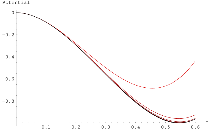
Figure 2: Plots of the tachyon effective potential $V_{L}(T)$ at level $L$, for $L$ between zero (uppermost curve) and 16 (lowermost curve). The curves for $L=6,10,12,14,16$ appear superimposed in the figure.

For our extrapolations, we focus on a interval for the tachyon vev around the non-perturbative vacuum. We take $0.54\leq T\leq 0.55$. The function $V^{(M)}_{L}(T)$, where $M$ is an even integer $\leq 16$, is the extrapolation ‘of order $M$’ of the tachyon effective action at level $L$, and is constructed as follows. We fix the dependence on $L$ by writing

$$V^{(M)}_{L}(T)=\sum_{n=0}^{M/2+1}\frac{a_{n}(T)}{(L+1)^{n}}\,,$$ (4.3)

for some coefficients functions $a_{n}(T)$. The functions $a_{n}(T)$ are determined by imposing the conditions

$$V^{(M)}_{L}(T)=V_{L}(T)\,,\qquad\;{\rm for\;}L=0,2,\cdots,M\,,\quad\quad\forall\;T\in[0.54,0.55]\,.$$ (4.4)

In other terms, we interpolate the $M/2+1$ values $\{V_{L}(T)|L=0,2,\dots M\}$ with a polynomial in $1/(L+1)$ that passes through all the data points.

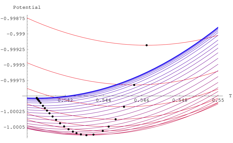
Figure 3: Plots of the order 16 estimates $V_{L}^{(16)}(T)$ for the effective tachyon potential, for some sample values of $L\geq 10$. The minimum of each curve is indicated by a black dot, which by definition has coordinates $(T^{(16)}_{L},E_{L}^{(16)})$. The isolated uppermost plot corresponds to $L=10$. To follow the curves from $L=10$ to $L=\infty$, focus on the position of the minima: as $L$ increases, the dot moves from right to left (i.e., the tachyon vev decreases). As $L\to\infty$, the curves crowd towards an asymptotic function with minimum at $(T_{\infty}^{(16)},E_{\infty}^{(16)})=(0.5405,-1.00003)$.

Figure 4: Plot of $E_{L}^{(16)}$ as a function of $1/L$. The black dots represent the exact values up to $L=18$ computed by direct level-truncation (Table 1, $(L,3L)$ scheme). To first approximation, the curve in the figure is roughly a parabola: since the energy overshoots -1 at $1/L=1/14\simeq 0.07$, we have a visual understanding of the position of the minimum of the energy around $1/L=(1/14)/2=1/28\simeq 0.036$.

	$L=4$	$L=6$	$L=8$	$L=10$
$M=4$	-0.98782176	-0.99546179	-0.99850722	-1.0000023
$M=6$		-0.99517712	-0.99798495	-0.99930406
$M=8$			-0.99793018	-0.99918359
$M=10$				-0.99918246
	$L=12$	$L=14$	$L=16$	$L=18$
$M=4$	-1.0008372	-1.0013461	-1.0016765	-1.0019017
$M=6$	-1.0000079	-1.0004169	-1.0006692	-1.0008317
$M=8$	-0.99982545	-1.0001796	-1.0003843	-1.0005057
$M=10$	-0.99982266	-1.0001750	-1.0003780	-1.0004979
$M=12$	-0.99982226	-1.0001739	-1.0003759	-1.0004947
$M=14$		-1.0001737	-1.0003755	-1.0004938
$M=16$			-1.0003755	-1.0004937
$M=18$				-1.0004937

Table 7: Estimates $E^{(M)}_{L}$ for the vacuum energy obtained from extrapolations of the effective tachyon potential, at various orders $M$ and for $L\leq 18$. Data in the $(L,3L)$ scheme. By definition, the diagonal entries $E^{(M=L)}_{L}$ coincide with the exact computation from direct level-truncation at level $(L,3L)$ (Table 1).

Our best estimate for the tachyon effective action at level $L$ is the function $V_{L}^{(16)}(T)$. Figure 3 shows the plots of $V_{L}^{(16)}(T)$ for $L$ between ten and infinity. The position of the minimum in each curve defines our order $M=16$ estimates $T^{(16)}_{L}$ and $E^{(16)}_{L}$ for the tachyon vev and vacuum energy at level $L$. We can follow very clearly the behavior of the minima as $L$ increases. The energy falls below -1, reaches its lowest point in $L=28$ curve, and then turns back to approach asymptotically the value $E^{(16)}_{\infty}=-1.00003$ ! In Figure 4 we see the same phenomenon in a plot of $E^{(16)}_{L}$ as a function of $1/L$.

It is interesting to consider how the extrapolations change as we vary $M$. Table 7 shows the estimates $E^{(M)}_{L}$ up to $L=18$, while Table 12 (appendix B) shows the analogous estimates for the tachyon vev. By construction, the diagonal entries $E^{(L)}_{L}$ and $T^{(L)}_{L}$ are simply the exact values obtained by direct level-truncation at level $L$. One can observe from the tables that the method has remarkable predictive power. For example, by only knowing level-truncation results up to level 10, one can obtain the prediction $E^{(10)}_{16}=-1.0003780$ for the energy at level 16, to be compared to the exact value $E_{16}=-1.0003755$. We thus feel quite comfortable in trusting the extrapolations even for $L$ large. Figure 1 and Table 2 (already discussed in the introduction) illustrate the main features of the larger $L$ results for the vacuum energy, for various $M$’s. It is pleasant to observe that, as $M$ increases, the estimates $L^{(M)}_{min}$ and $E^{(M)}_{min}$ (Table 2) quickly reach stable values, while $E^{(M)}_{\infty}$ steadily approaches minus one.

It is remarkable that extrapolations to higher levels work so well. The data have a smooth and predictable dependence on $L$, which is very well captured by polynomials in $1/L$. This property was not a priori obvious, and indeed it appears to be true only for $(L,3L)$ data, as we shall see in section 4.3.

4.2 Comparison with Straightforward Extrapolations

The method just described appears to work remarkably well. To which extent does the success of the method depend on the sophisticated idea of extrapolating the functional form of the tachyon effective action? We can answer this question by considering the more straightforward procedure of simply extrapolating the values of the vacuum energies $E_{L}$ (as opposed to the full functions $V_{L}(T)$). We define the ‘straightforward’ order $M$ estimate ${\widetilde{E}}^{(M)}_{L}$ at level $L$ by considering the data $\{E_{L}|0\leq L\leq M\}$, and interpolating them with a polynomial in $1/(L+1)$ of maximum degree. (This is in complete analogy with (4.3)). The results for $L\leq 18$ in the $(L,3L)$ scheme are presented in Table 8, while in Table 9 we give the extrapolations to $L=\infty$. We see that for $M<10$, the more sophisticated method gives much more accurate predictions (compare Table 7 and Table 8: for example $E^{(8)}_{18}$, ${\widetilde{E}}^{(8)}_{18}$ and the exact value $E_{18}^{(18)}$). However for $M>10$ there is no significant difference between the two procedures. We also compared the results for the individual coefficients of the tachyon string field obtained with the two procedures, and found a very similar pattern.

	$L=4$	$L=6$	$L=8$	$L=10$
$M=4$	-0.98782176	-0.99730348	-1.0020443	-1.0048888
$M=6$		-0.99517712	-0.99845611	-1.0002959
$M=8$			-0.99793018	-0.99921882
$M=10$				-0.99918246
	$L=12$	$L=14$	$L=16$	$L=18$
$M=4$	-1.0067851	-1.0081397	-1.0091556	-1.0099457
$M=6$	-1.0014693	-1.0022814	-1.0028762	-1.0033304
$M=8$	-0.99991100	-1.0003187	-1.0005753	-1.0007448
$M=10$	-0.99982332	-1.0001767	-1.0003811	-1.0005023
$M=12$	-0.99982226	-1.0001738	-1.0003758	-1.0004946
$M=14$		-1.0001737	-1.0003755	-1.0004939
$M=16$			-1.0003755	-1.0004937
$M=18$				-1.0004937

Table 8: The estimates ${\widetilde{E}}^{(M)}_{L}$ for the vacuum energy in the $(L,3L)$ scheme, obtained with the ‘straightforward’ polynomial extrapolation in $1/(L+1)$.

We conclude that with the sophisticated procedure one can achieve remarkable accuracy even for small $M$, where a naive extrapolation would work quite poorly. However if one is willing to perform level-truncation up to level 12 or above, the simpler extrapolation procedure is equally effective.

4.3 $(L,3L)$ versus $(L,2L)$

	$(L,3L)$	$(L,2L)$
$M=6$	-0.998698	-0.988625
$M=8$	-0.999784	-1.00261
$M=10$	-1.00010	-0.999316
$M=12$	-1.00008	-1.00048
$M=14$	-1.00004	-0.999655
$M=16$	-1.00003	-1.00057

Table 9: The estimates ${\widetilde{E}}^{(M)}_{\infty}$ for the asymptotic vacuum energy in the $(L,3L)$ and $(L,2L)$ schemes, obtained with the ‘straightforward’ polynomial extrapolation in $1/(L+1)$.

Figure 5: Plot of the results in Table 9. The continuous line represents the $(L,3L)$ results, while the dashed line represents the $(L,2L)$ results.

All the extrapolations described so far are for results in the $(L,3L)$ scheme. We have investigated the data in the $(L,2L)$ scheme and concluded that their behavior as a function of $L$ is not nearly as smooth: as a consequence, extrapolations to higher levels are less reliable. A glance at Table 9 and Figure 5 is sufficient to illustrate our point. We are comparing the ‘straightforward’ extrapolations of the vacuum energy to $L=\infty$, for various $M$’s, obtained with data in the $(L,3L)$ scheme, with the analogous quantities in the $(L,2L)$ scheme. While the $(L,3L)$ data have a really smooth dependence on $M$ and converge nicely to -1, the $(L,2L)$ data have a much more irregular behavior. A similar pattern is observed for extrapolations at finite $L$: estimates ${\widetilde{E}}^{(M)}_{L}$ of exact results at level $L\leq 18$ are not nearly as accurate in the $(L,2L)$ scheme as they are in the $(L,3L)$ scheme. An analogous behavior is found in comparing $(L,3L)$ and $(L,2L)$ data for the tachyon vev. We have also repeated for $(L,2L)$ data the full analysis based on extrapolations of the tachyon effective action, and found no improvement with respect to the straightforward extrapolations shown in Table 9.

It would be interesting to explain these findings from an analytic point of view. The $(L,3L)$ scheme can be understood as a cut-off procedure in which only the kinetic term of the OSFT action is changed, such to give an infinite mass to modes with level higher than $L$. On the other hand, in the $(L,2L)$ scheme both the kinetic and the cubic term of the action are changed. This may explain why $(L,3L)$ data have a simpler dependence on $L$.

5 Patterns of the Siegel Gauge Tachyon Condensate

The individual coefficients of the tachyon condensate can also be extrapolated to higher levels. The more sophisticated method that we use is the following: We solve the classical equations of motion at level $L$ and express all higher modes $\widetilde{\Psi}_{L}$ as functions of the tachyon vev $T$ (see (A.12)). We then perform an extrapolation of these functions of $T$ using a polynomial in $1/L$ of maximum degree: this defines in the usual way the order $M$ estimates $\widetilde{\Psi}^{(M)}_{L}[T]$. Finally by setting $T=T_{L}$ we obtain extrapolations for the full tachyon string field. Tables 14 and 15 (appendix B) contain the extrapolations to $L\leq 18$ of the first two higher modes. In Table 13 we give the $M=16$ results for the extrapolations to $L=\infty$ obtained using this method.

We are finally in the position to look for analytic patterns in the tachyon condensate, in particular checking in a more reliable way the patterns observed in [37]. This was one of the motivations of our work.

The Tachyon Vev

Figure 6: Plot of the estimate $T^{(16)}_{L}$ for tachyon vev as a function of $1/L$. The dots represent the exact values $T_{L}$ for $L=2\dots 18$. The dashed line represents the value $T_{HS}=\sqrt{3}/\pi$.

Figure 6 is a plot of the estimate for the tachyon vev as a function of $1/L$. The asymptotic value is $T^{(16)}_{\infty}\simeq 0.5405$. Clearly the conjecture [29] for an exact value $T_{HS}=\sqrt{3}/\pi$ is falsified.

Universal Ghost Coefficients

$L$	$r_{1,1}$	$r_{3,1}$	$r_{5,1}$	$r_{3,3}$	$r_{7,1}$	$r_{5,3}$
2	0.349483
4	0.375042	-0.102499
6	0.386571	-0.104743	0.0547758	0.0208371
8	0.393062	-0.105966	0.05544	0.0209129	0.0358037	0.014195
10	0.397214	-0.106707	0.0558499	0.0209927	0.0361037	0.0142012
12	0.400096	-0.107201	0.0561103	0.0210499	0.0363031	0.0142291
14	0.402212	-0.107553	0.0562894	0.0210917	0.0364338	0.0142521
16	0.403832	-0.107818	0.0564199	0.0211232	0.0365254	0.0142701
18	0.405111	-0.108023	0.0565194	0.0211478	0.0365932	0.0142843
$\infty$	0.4160	-0.1097	0.05728	0.02135	0.03739	.01456
$conj$	0.407407	-0.109739	0.0577148	0.021328	0.037483	.01439

Table 10: $(L,3L)$ numerical results for the pattern coefficients $r_{n,m}$ for the tachyon condensate string field, and their conjectured values. The $L=\infty$ results are obtained from the $M=16$ extrapolation procedure based on the effective tachyon potential.

The most accurate pattern discovered in [37] is the remarkable universality of certain ghost coefficients. If one normalizes the tachyon mode to one, then the coefficients $r_{n,m}$ of the modes $c_{-n}b_{-m}c_{1}|0\rangle$ (with $n$ and $m$ odd) appear to be the same for all known OSFT solutions. Assuming that this is the case, an analytic prediction for these coefficients is possible by looking at infinitesimal OSFT solutions corresponding to exactly marginal deformations of the BCFT.

We reproduce our results for these coefficients for the tachyon condensate in Table 10 and in Table 16 (this latter table is in appendix B). There is certainly a striking pattern. In particular, the results of Table 16 show that the pattern persists in the higher-level modes that were not explored in [37]. However the value for $r_{1,1}$ is puzzling. This result has not improved with respect to the $L=12$ data already available in [37], and the $2\%$ difference from the conjectured value would seem like a real one.

Although we hesitate to assign a precise error to our extrapolations to $L=\infty$, it seems that this error should be smaller than than $2\%$. Indeed all the properties that we know for sure to be exact (the quadratic identities, the out-of-Siegel equations and of course the value of the vacuum energy), are obeyed with an accuracy of order $10^{-5}$ in the $M=16$ extrapolations.

	${\cal T}_{Siegel}$	$\Phi\;\;\;\;$
$L_{-2}$	.1058	0.1069
$L_{-4}$	-.009343	-0.009476
$L_{-2}L_{-2}$	-.001260	-0.001221
$L_{-6}$	.002648	0.002691
$L_{-3}L_{-3}$	.0000135	0.0000143
$L_{-4}L_{-2}$	.000575	0.000594
$L_{-2}L_{-2}L_{-2}$	-.000009	-0.000016

Table 11: The left column shows the normalized matter coefficients of the tachyon condensate string field for $L=\infty$ (from Table 13). The right columns shows the corresponding coefficients for the ghost number zero string field, obtained from an extrapolation to $L=\infty$ of data up to $L=14$, with a maximal polynomial in $1/L$.

$L_{0}\,{\cal T}$ factorization

In [37] it was observed that the string field $L_{0}\,{{\cal T}_{Siegel}}$ is approximately factored into a matter times a ghost component. In view of our more precise data, we definitely conclude that this is just a rough pattern, as already believed in [37]. Indeed the pattern is seen to get worse in the $L=\infty$ extrapolations. Let us give a couple of examples. Assuming factorization, the normalized coefficient of $L^{m}_{-2}c_{-1}|0\rangle$ can be obtained by multiplying the two normalized coefficients of $L^{m}_{-2}|0\rangle$ and $c_{-1}|0\rangle$. In [37], using the numerical values at level $(10,30)$, this procedure gave a prediction with a $4\%$ error; with the $L=\infty$ data in Table 13, the error is increased to $8\%$. Similarly, applying the same procedure to $L^{m}_{-4}c_{-1}|0\rangle$, one finds only a $0.1\%$ error at level $(10,30)$, but a $1\%$ error using the values in Table 13.

Correspondence with Ghost Number Zero

The last pattern noticed in [37] is a surprising coincidence between the OSFT equation and the equation

$$(L_{0}-1)\Phi+\Phi*\Phi=0\,,$$ (5.5)

where $\Phi$ is a ghost number zero field. This equation can be solved in the universal space spanned by total Virasoro’s $L_{-n}$ acting on the vacuum. It was found that the coefficients of the terms $L_{-k_{1}}\cdots L_{-k_{n}}|0\rangle$ in the solution of (5.5) are strikingly close to the normalized coefficients of the matter modes $L^{m}_{-k_{1}}\cdots L^{m}_{-k_{n}}c_{1}|0\rangle$ of ${\cal T}_{Siegel}$. However the pattern is somewhat irregular and does not appear to systematically improve with level. This is confirmed by our more precise data, a sample of which is presented in Table 11. There is no clear improvement with respect to the data in [37], and we confirm the conclusion that this is likely only a ‘quasi-pattern’.

All in all, the patterns of [37] are still present in our more precise data, and one cannot help the feeling that they hint at some analytic clue. However we seem to conclude that all these patterns are not exact properties, with the possible exception of the universality conjecture for certain ghost coefficients. This last conjecture is generally well obeyed, but we found a disturbing discrepancy for the $c_{-1}|0\rangle$ mode.

6 Concluding Remarks

Our results support the idea that level-truncation is a completely reliable approximation scheme for OSFT, with a convergent limit as the level is sent to infinity. All available exact predictions (notably the value of the vacuum energy) are accurately confirmed by the data. No inconsistencies seem to arise from the fact that gauge-invariance is broken at finite level, indeed we found strong evidence that it is smoothly restored as $L\to\infty$. Quantities computed in level-truncation exhibit a predictable dependence on level which is very well approximated by polynomials in $1/L$ (at least for the $(L,3L)$ scheme). This allows reliable extrapolations to higher levels. Combining this observation with efficient computer algorithms based on conservation laws [4], we have developed very powerful numerical tools to study OSFT.

In this paper we have focused on the universal subspace and obtained accurate data for the tachyon condensate. An obvious direction for further research is to use our results to learn about the kinetic term around the tachyon vacuum. The nature of this kinetic term is still rather mysterious. No perturbative open string states are expected to be present, and numerical evidence for this has already been obtained [31]. Our data will allow a more precise analysis, and hopefully give new analytic clues.

The most intriguing aspects of the non-perturbative vacuum are related to the elusive closed string states. In OSFT, amplitudes for external closed strings (on a surface with a least one boundary) are given by correlation functions of certain gauge-invariant open string functionals [45, 46, 47, 11]. It would be very interesting to compute such amplitudes in the non-perturbative vacuum. This should shed some light on the mechanism by which open string moduli are frozen in the tachyon vacuum, but closed string moduli are still present. There are promising ideas for how this may come about [11, 48, 49], but the actual mechanism realized in OSFT is still unknown.

Another avenue for future work is the application of our methods to more general classical solutions. It will be straightforward to extend our algorithms to include the matter states necessary to construct non-universal solutions, e.g. tachyon lump solutions [23] and Wilson line solutions [25]. It would also be very nice to investigate numerically time-dependent solutions, and demonstrate the existence of tachyon matter [50] in OSFT. The study of several classical solutions will help to build the intuition that is needed for analytic progress.

We hope that the precise data presented in this paper will encourage other physicists to think about analytic approaches to OSFT. Our analysis of the ‘patterns’ of the tachyon condensate throws some doubt even on the most robust conjecture proposed in [37], although it does not rule it out completely. The search for analytic clues in OSFT solutions is still very open. Yet we feel that our numbers for the tachyon string field must possess some hidden beauty, to be unveiled when an exact solution is found.

Acknowledgments.

It is a pleasure to thank Ashoke Sen, Wati Taylor and Barton Zwiebach for their constant interest in our work and for many detailed discussions at various stages of this project. This material is based upon work supported by the National Science Foundation Grant No. PHY-9802484. Any opinions, findings, and conclusions or recommendations expressed in this material are those of the authors and do not necessarily reflect the views of the National Science Foundation.

Appendix A The Numerical Algorithms

In this appendix we explain some technical details about the algorithms that we have used to compute the universal star products and find the tachyon solution in level truncation.

A.1 Star Products from Conservation Laws

The strategy for evaluating star products using conservation laws is explained in detail in [4]. Each Fock state in ${\cal H}_{univ}^{(1)}$ can be represented as a string of negatively moded ghost or Virasoro generators acting on the zero-momentum tachyon $c_{1}|0\rangle$. The triple product of three such states is evaluated recursively by converting a negatively moded generator on one state space to a sum of positively moded generators acting on all three state spaces,

$$\langle A_{-k}\Phi_{1},\Psi_{2},\Psi_{3}\rangle=$$ (A.1)

$$r_{k}\langle\Phi_{1},\Psi_{2},\Psi_{3}\rangle+\langle\sum_{n\geq 0}\alpha_{n}^{k}A_{n}\Phi_{1},\Psi_{2},\Psi_{3}\rangle+\langle\Phi_{1},\sum_{n\geq 0}\beta_{n}^{k}A_{n}\Psi_{2},\Psi_{3}\rangle+\langle\Phi_{1},\Psi_{2},\sum_{n\geq 0}\gamma_{n}^{k}A_{n}\Psi_{3}\rangle\,,$$

where $A_{-k}$ is any constructor symbol and the coefficients appearing in this ‘conservation law’ are computed from the geometry of the Witten vertex [4]. All triple products in ${\cal H}^{(1)}_{univ}$ are thus reduced to the coupling $\langle c_{1},c_{1},c_{1}\rangle$ of three tachyons.

Once the triple products are known, star products are easily obtained by inverting the non-degenerate bpz inner product. If $\{\Psi_{i}\}$ is a Fock basis for ${\cal H}^{(1)}_{univ}$, we define the dual basis $\{\Psi^{i}\}$ of ${\cal H}^{(2)}_{univ}$ by the bpz pairing

$$\langle\Psi_{i},\Psi^{j}\rangle=\delta_{i}^{j}\,.$$ (A.2)

Then

$$\Psi_{i}*\Psi_{j}\equiv\sum_{k}\langle\Psi_{i},\Psi_{j},\Psi_{k}\rangle\,\Psi^{k}\,.$$ (A.3)

We automated this algorithm on a C++ computer code. We briefly highlight some features of our implementation:

• We use the factorization of the star product into matter and ghost sectors. The algorithm to find the triple products is executed separately in the two subsectors.

• We use cyclic and twist symmetry of the vertex to reduce the computation to triple products $\langle\Psi_{i},\Psi_{j},\Psi_{k}\rangle$ with a canonical ordering $i\leq j\leq k$.

• While in the matter sector the algorithm can be implemented in a straightforward way, in the ghost sector we need to face a slight complication. We are ultimately interested in triple products of ghost number one states, but the use of fermionic ghost conservation laws necessarily brings us outside the ghost number one subspace. We found it most efficient to use only conservation laws for the $b_{-k}$ oscillators. A single application of a $b$-ghost conservation law reduces the evaluation of a $\langle 1,1,1\rangle$ product (ghost number one in all three slots) to a sum of terms of the form $\langle 1,1,1\rangle$ and $\langle 0,1,2\rangle$. Products of this latter type can be treated by applying a $b$-conservation law to the first state (of ghost number zero), obtaining a sum of terms $\langle 1,1,1\rangle$ and again (after cyclic rearrangement) $\langle 0,1,2\rangle$. It is easy to show that this algorithm always terminates on the product of three tachyons. So we see that we only need to consider triple products of the form $\langle 0,1,2\rangle$ besides the standard products $\langle 1,1,1\rangle$.

• After each application of a conservation law, the resulting triple products on the r.h.s of (LABEL:conslaw) are processed using the Virasoro algebra or the ghost commutation relations, till all states are reduced to the Fock basis (2.6) with the canonical ordering $j_{1}\geq\dots\geq j_{p}$, $k_{1}\geq\dots\geq k_{q}$, $l_{1}\geq\dots\geq l_{r}$. The evaluation of expressions like $L_{k}L_{-n_{1}}\cdots L_{-n_{i}}c_{1}|0\rangle$, with $n_{1}\geq n_{2}\cdots\geq n_{i}$ (and similarly for the ghosts) is thus a basic elementary operation. There is a critical gain in efficiency in evaluating beforehand all such expressions (up to the desired maximum level) and reading the results from a file, rather then re-computing them each time. The size of such a file grows only linearly with the number of modes, whereas the table of triple products grows cubically, so this strategy is not problematic from the point of view of memory occupation.

This algorithm can be easily extended to evaluate more general star products of string fields belonging to a larger space than ${\cal H}_{univ}$, for example the space relevant for tachyon lump solutions [23] or Wilson line solutions [25]. One needs to enlarge the algebra of matter operators and consider the appropriate conservation laws.

A.2 Solving the Equations of Motion

Once all triple products at level $L$ have been computed, the evaluation of the star product of two Siegel gauge string fields at level $L$ involves $O(N_{L}^{3})$ algebraic operations. It is clearly desirable to have an algorithm to solve the classical eom’s that requires as few star products as possible. We tried various options, which can all be represented as a recursive procedure $\Psi^{(n+1)}=F(\Psi^{(n)})$, where $\Psi=F(\Psi)$ implies that $\Psi$ is a solution.

The most obvious idea is to invert the kinetic term in Siegel gauge and define

$$F(\Psi)=-\frac{b_{0}}{L_{0}}\,(\Psi*\Psi)\,.$$ (A.4)

Clearly this iteration cannot converge since $F(\lambda\Psi)=\lambda^{2}F(\Psi)$. There is a simple way to fix this problem, defining

$$\widetilde{F}(\Psi)=\left(\frac{T[\Psi]}{T[F(\Psi)]}\right)^{2}\,F(\Psi)\,,$$ (A.5)

where $T[\Phi]$ indicates the coefficient of $c_{1}|0\rangle$ in the string field $\Phi$. Unfortunately the algorithm based on the recursion $\widetilde{F}$ still fails to converge, and generically falls into stable two-cycles. An improved recursion is

$$F_{\alpha}(\Psi)=\alpha\,\Psi+(\alpha-1)\frac{b_{0}}{L_{0}}\Psi*\Psi\,$$ (A.6)

where $\alpha$ is a real number which is chosen randomly in some reasonable interval (say $0.2<\alpha<0.8$) at each iteration step. This randomization breaks the cycles and the algorithm converges to a unique solution in about 20-30 steps. (The algorithm stops when the eom’s are satisfied with the same accuracy as the accuracy of double-precision variables in C++, which have 15 significant digits). This algorithm is very robust with respect to the choice of the starting point $\Psi_{0}$, in fact at any given level $L$ we found only one non-trivial solution.

A more efficient approach is the standard Newton algorithm. Recall that given a system of $N$ algebraic equations in $N$ variables, $f_{i}[x_{\alpha}]=0$, $1\leq i,\alpha\leq N$, the Newton recursion is

$$x_{\alpha}^{(n+1)}=x_{\alpha}^{(n)}-M^{-1}_{\alpha i}[x^{(n)}]f_{i}[x^{(n)}]$$ (A.7)

where the matrix $M_{i\alpha}[x]$ is defined as

$$M_{i\alpha}[x]\equiv\frac{\partial f_{i}}{\partial x_{\alpha}}\,.$$ (A.8)

In our case, the truncated Siegel equations of motion are a system of $N_{L}$ algebraic equations in $N_{L}$ variables (Table 3) and this method can be directly applied. It is interesting to write the Newton algorithm as a recursion for the Siegel string field itself. One finds the compact expression

$$\Psi^{(n+1)}=Q_{\Psi^{(n)}}^{-1}(\Psi^{(n)}*\Psi^{(n)})\,.$$ (A.9)

Here the operator $Q_{\Psi}$ is defined by

$$Q_{\Psi}\,\Phi\equiv Q_{B}\Psi+\Psi*\Phi+\Phi*\Psi$$ (A.10)

for any ghost number one string field $\Phi$. The inverse operator $Q^{-1}_{\Psi}$ is naturally defined by projecting onto the Siegel subspace. In other terms, for any ghost number two string field $\Sigma$, we look for the ghost number one string field $Q^{-1}_{\Psi}\Sigma$ that obeys

$$b_{0}\,(Q^{-1}_{\Psi}\Sigma)=0\,,\quad c_{0}b_{0}\,\Sigma=c_{0}b_{0}\,Q_{\Psi}(Q^{-1}_{\Psi})\,\Sigma\,.$$ (A.11)

The operator $Q_{\Psi}$ has a natural physical interpretation: If $\Psi$ is a solution of the OSFT eom’s, then $Q_{\Psi}$ is the new BRST operator obtained expanding the OSFT action around $\Psi$. Thus as we approach the fixed point of the Newton recursion, $Q_{\Psi^{(n)}}$ becomes a better and better approximation to the BRST operator around the tachyon vacuum.

In level-truncation, the action of the operator $Q_{\Psi}$ in the Siegel subspace is represented by an $N_{L}\times N_{L}$ matrix. Since there is an order $O(N_{L}^{3})$ algorithm to invert a matrix, the Newton recursion is not significantly more time-expensive than the evaluation of a single star product. The Newton algorithm is very fast, effectively squaring the accuracy at each step, and the solution is reached in four or five iterations. On our pc, the complete algorithm (computing the vertices from scratch and finding the tachyon solution) takes less than 10 seconds at level (10,20), and less than a minute at level (12,36)! There is however a rather critical dependence on the initial conditions: one finds convergence only from a starting point sufficiently close to the solution (it is enough to take e.g. $\Psi^{(0)}=0.5\,c_{1}|0\rangle$).

We compared the solution obtained with the Newton method with the solution found with the alternative algorithm described above, finding exact agreement up to level 16. (At level 18 the recursion (A.6) runs too slowly on our pc). This gives a strong check on the correctness of the solutions. As another check, we compared our results at level (10,20) with the results of Moeller and Taylor [20], finding agreement to the tenth significant digit.

A.3 Tachyon Effective Action

To compute the tachyon effective action, we write the string field as

$$\Psi_{L}=T\,c_{1}|0\rangle+\widetilde{\Psi}_{L}\,,$$ (A.12)

where $\widetilde{\Psi}_{L}$ contains all the modes up to level $L$, except $c_{1}|0\rangle$. For a given numerical value of of the variable $T$, we solve the classical OSFT equations of motion for all the higher modes, using the Newton method. This gives $\Psi_{L}[T]=Tc_{1}|0\rangle+\widetilde{\Psi}_{L}[T]$ as a function of $T$. Plugging $\Psi_{L}[T]$ into the OSFT action we obtain the effective tachyon potential $V_{L}(T)$.

The Newton algorithm that finds the solution $\widetilde{\Psi}_{L}[T]$ fails to converge if the variable $T$ is outside an interval $[T_{L}^{min},T_{L}^{max}]$. We find for example $T^{min}_{16}\sim-0.1$ and $T^{max}_{16}\sim 0.7$ (notice that both the tachyon vacuum and the perturbative vacuum are safely inside the convergence region). The failure of the numerical algorithm can be explicitly traced to the existence of other branches in the tachyon effective action. This phenomenon has been studied in [20, 35], where it has also been related to the non-perturbative failure of the Siegel gauge condition. In this paper we only need $V_{L}(T)$ in an interval around the non-perturbative vacuum, which we take to be $0.54\leq T\leq 0.55$. We postpone a more detailed investigation of the global behavior of the tachyon potential.

Appendix B Some Further Numerical Data

	$L=4$	$L=6$	$L=8$	$L=10$
$M=4$	0.54839904	0.54849677	0.54814406	0.54777626
$M=6$		0.54793242	0.54711284	0.54639593
$M=8$			0.54705245	0.54626520
$M=10$				0.54626093
	$L=12$	$L=14$	$L=16$	$L=18$
$M=4$	0.54745869	0.54719393	0.54697362	0.54678893
$M=6$	0.54581507	0.54534684	0.54496539	0.54465027
$M=8$	0.54561932	0.54509452	0.54466463	0.54430807
$M=10$	0.54560864	0.54507682	0.54464004	0.54427703
$M=12$	0.54560809	0.54507524	0.54463714	0.54427267
$M=14$		0.54507515	0.54463683	0.54427204
$M=16$			0.54463682	0.54427198
$M=18$				0.54427196

Table 12: Estimates $T^{(M)}_{L}$ for the tachyon vev obtained from extrapolations of the effective tachyon potential, at various orders $M$ and for $L\leq 18$. Data in the $(L,3L)$ scheme. By definition, the diagonal entries $T^{(M=L)}_{L}$ coincide with the exact computation from direct level-truncation at level $(L,3L)$ (Table 4).

Matter	Ghost	$L=\infty$	$L=18$
		.5405	0.5443
	$b_{-1}c_{-1}$	-0.2248	-0.2205
$L^{m}_{-2}$		0.05721	0.05726
	$b_{-1}c_{-3}$	0.05928	0.05879
	$b_{-2}c_{-2}$	0.03650	0.03564
	$b_{-3}c_{-1}$	0.01976	0.01960
$L^{m}_{-2}$	$b_{-1}c_{-3}$	0.008627	0.008197
$L^{m}_{-4}$		-0.005049	-0.005079
$L^{m}_{-2}L^{m}_{-2}$		-0.000681	-0.000661
	$b_{-1}c_{-5}$	-0.03091	-0.03076
	$b_{-2}c_{-4}$	-0.01976	-0.01941
	$b_{-3}c_{-3}$	-0.01152	-0.01151
	$b_{-2}b_{-1}c_{-2}c_{-1}$	-0.008626	-0.008316
	$b_{-4}c_{-2}$	-0.00988	-0.009704
	$b_{-5}c_{-1}$	-0.00618	-0.006152
$L^{m}_{-2}$	$b_{-1}c_{-3}$	-0.003702	-0.003605
$L^{m}_{-2}$	$b_{-2}c_{-2}$	-0.003186	-0.003056
$L^{m}_{-2}$	$b_{-1}c_{-1}$	-0.001234	-0.001202
$L^{m}_{-3}$	$b_{-1}c_{-2}$	-0.000076	-0.0000775
$L^{m}_{-3}$	$b_{-2}c_{-1}$	-0.000038	-0.0000387
$L^{m}_{-4}$	$b_{-1}c_{-1}$	-0.0012	-0.001242
$L^{m}_{-2}L^{m}_{-2}$	$b_{-1}c_{-2}$	-0.000248	-0.000215
$L^{m}_{-6}$		0.001434	0.001446
$L^{m}_{-3}L^{m}_{-3}$		0.0000075	0.0000075
$L^{m}_{-4}L^{m}_{-2}$		0.000311	0.000310
$L^{m}_{-2}L^{m}_{-2}L^{m}_{-2}$		-0.0000049	-0.0000065

Table 13: Asymptotic values for the first coefficients of the tachyon condensate string field, compared with the $L=18$ data. The $L=\infty$ results are obtained from the $M=16$ extrapolation procedure based on the effective tachyon potential. Data in the $(L,3L)$ scheme.

	$L=4$	$L=6$	$L=8$	$L=10$
$M=4$	-0.20567285	-0.21119493	-0.21392087	-0.21552208
$M=6$		-0.21181486	-0.21499106	-0.21690691
$M=8$			-0.21502535	-0.21697620
$M=10$				-0.21698254
	$L=12$	$L=14$	$L=16$	$L=18$
$M=4$	-0.21656852	-0.21730328	-0.21784642	-0.21826369
$M=6$	-0.21818110	-0.21908711	-0.21976325	-0.22028663
$M=8$	-0.21827982	-0.21920964	-0.21990503	-0.22044413
$M=10$	-0.21829559	-0.21923573	-0.21994128	-0.22048993
$M=12$	-0.21829570	-0.21923600	-0.21994171	-0.22049051
$M=14$		-0.21923603	-0.21994180	-0.22049069
$M=16$			-0.21994181	-0.22049069
$M=18$				-0.22049069

Table 14: Estimates for the vev of $c_{-1}|0\rangle$, obtained from extrapolations of the effective tachyon potential, at various orders $M$ and for $L\leq 18$. Data in the $(L,3L)$ scheme. By definition, the diagonal entries coincide with the exact computation from direct level-truncation at level $(L,3L)$ (Table 4).

	$L=4$	$L=6$	$L=8$	$L=10$
$M=4$	0.056923526	0.057062755	0.057068423	0.057045668
$M=6$		0.057143493	0.057209039	0.057229308
$M=8$			0.057214101	0.057239805
$M=10$				0.057241066
	$L=12$	$L=14$	$L=16$	$L=18$
$M=4$	0.057018045	0.056991677	0.056968053	0.056947298
$M=6$	0.057233609	0.057231744	0.057227479	0.057222387
$M=8$	0.057248895	0.057251070	0.057250189	0.057247946
$M=10$	0.057252093	0.057256442	0.057257742	0.057257584
$M=12$	0.057252005	0.057256182	0.057257253	0.057256834
$M=14$		0.057256190	0.057257279	0.057256887
$M=16$			0.057257279	0.057256886
$M=18$				0.057256885

Table 15: Estimates for the vev of $L^{m}_{-2}c_{1}|0\rangle$, obtained from extrapolations of the effective tachyon potential, at various ‘orders’ $M$ and for $L\leq 18$. Data in the $(L,3L)$ scheme. By definition, the diagonal entries coincide with the exact computation from direct level-truncation at level $(L,3L)$ (Table 4).

	$L=10$	$L=12$	$L=14$	$L=16$	$L=18$	$conj$
$r_{9,1}$	0.0259407	0.0261085	0.0262255	0.0263037	0.0263594	0.027063
$r_{7,3}$	0.0104886	0.0104825	0.0104948	0.0105063	0.0105159	0.0105868
$r_{5,5}$	0.00658638	0.0065773	0.00658224	0.00658778	0.00659265	0.0066192
$r_{11,1}$		-0.0200117	-0.0201181	-0.0201948	-0.0202469	-0.0208326
$r_{9,3}$		–0.00818159	-0.00817378	-0.00818	-0.00818657	-0.00824041
$r_{7,5}$		-0.00525767	-0.00524794	-0.00524929	-0.00525185	-0.00526601
$r_{13,1}$			0.0161045	0.0161778	0.0162318	0.0167396
$r_{11,3}$			0.00662999	0.00662276	0.0066262	0.0066689
$r_{9,5}$			0.00431978	0.00431134	0.00431141	0.00431915
$r_{7,7}$			0.00315946	0.00315272	0.00315241	0.0031549
$r_{15,1}$				-0.0133607	-0.0134141	-0.013871
$r_{13,3}$				-0.0055259	-0.00551968	-0.005553
$r_{11,5}$				-0.00363327	-0.00362626	-0.003629

Table 16: $(L,3L)$ numerical results for the pattern coefficients $r_{n,m}$ for the tachyon condensate.

References

- [1] A. Sen, Int. J. Mod. Phys. A14, 4061 (1999) [hep-th/9902105]; hep-th/9904207.
- [2] A. Sen, “Universality of the tachyon potential”, JHEP 9912, 027 (1999) [hep-th/9911116].
- [3] E. Witten, “Noncommutative Geometry And String Field Theory,” Nucl. Phys. B 268, 253 (1986).
- [4] L. Rastelli and B. Zwiebach, “Tachyon potentials, star products and universality,” JHEP 0109, 038 (2001) [arXiv:hep-th/0006240].
- [5] V. A. Kostelecky and R. Potting, Phys. Rev. D 63, 046007 (2001) [hep-th/0008252]. L. Rastelli, A. Sen and B. Zwiebach, Adv. Theor. Math. Phys. 5, 393 (2002) [arXiv:hep-th/0102112]; JHEP 0111, 035 (2001) [arXiv:hep-th/0105058]; JHEP 0111, 045 (2001) [arXiv:hep-th/0105168]. D. J. Gross and W. Taylor, JHEP 0108, 009 (2001) [arXiv:hep-th/0105059]; JHEP 0108, 010 (2001) [arXiv:hep-th/0106036]. D. Gaiotto, L. Rastelli, A. Sen and B. Zwiebach, JHEP 0204, 060 (2002) [arXiv:hep-th/0202151]. M. Schnabl, arXiv:hep-th/0201095; arXiv:hep-th/0202139. L. Bonora, D. Mamone and M. Salizzoni, Nucl. Phys. B 630, 163 (2002) [arXiv:hep-th/0201060]; JHEP 0204, 020 (2002) [arXiv:hep-th/0203188]. E. Fuchs, M. Kroyter and A. Marcus, JHEP 0209, 022 (2002) [arXiv:hep-th/0207001].
- [6] I. Bars, Phys. Lett. B 517, 436 (2001) [arXiv:hep-th/0106157]. Bars and Y. Matsuo, Phys. Rev. D 65, 126006 (2002) [arXiv:hep-th/0202030]; Phys. Rev. D 66, 066003 (2002) [arXiv:hep-th/0204260].
- [7] L. Rastelli, A. Sen and B. Zwiebach, “Star algebra spectroscopy,” JHEP 0203, 029 (2002) [arXiv:hep-th/0111281].
- [8] M. R. Douglas, H. Liu, G. Moore and B. Zwiebach, “Open string star as a continuous Moyal product,” JHEP 0204, 022 (2002) [arXiv:hep-th/0202087].
- [9] B. Feng, Y. H. He and N. Moeller, JHEP 0204, 038 (2002) [arXiv:hep-th/0202176]; JHEP 0205, 041 (2002) [arXiv:hep-th/0203175]. B. Chen and F. L. Lin, Nucl. Phys. B 637, 199 (2002) [arXiv:hep-th/0203204]; arXiv:hep-th/0204233. D. M. Belov, arXiv:hep-th/0204164. T. G. Erler, arXiv:hep-th/0205107. D. M. Belov and A. Konechny, arXiv:hep-th/0207174; arXiv:hep-th/0210169. E. Fuchs, M. Kroyter and A. Marcus, arXiv:hep-th/0210155. D.M. Belov, arXiv:hep-th/0210199.
- [10] L. Rastelli, A. Sen and B. Zwiebach, “String field theory around the tachyon vacuum,” Adv. Theor. Math. Phys. 5, 353 (2002) [arXiv:hep-th/0012251].
- [11] D. Gaiotto, L. Rastelli, A. Sen and B. Zwiebach, “Ghost structure and closed strings in vacuum string field theory,” arXiv:hep-th/0111129.
- [12] Y. Okawa, “Open string states and D-brane tension from vacuum string field theory,” JHEP 0207, 003 (2002) [arXiv:hep-th/0204012].
- [13] H. Hata and T. Kawano, JHEP 0111, 038 (2001) [arXiv:hep-th/0108150]. L. Rastelli, A. Sen and B. Zwiebach, JHEP 0202, 034 (2002) [arXiv:hep-th/0111153]. H. Hata, S. Moriyama and S. Teraguchi, JHEP 0202, 036 (2002) [arXiv:hep-th/0201177]. H. Hata and H. Kogetsu, JHEP 0209, 027 (2002) [arXiv:hep-th/0208067].
- [14] K. Okuyama, JHEP 0201, 043 (2002) [arXiv:hep-th/0111087]; JHEP 0201, 027 (2002) [arXiv:hep-th/0201015]; JHEP 0203, 050 (2002) [arXiv:hep-th/0201136]. T. Okuda, Nucl. Phys. B 641, 393 (2002) [arXiv:hep-th/0201149]. Y. Imamura, JHEP 0207, 042 (2002) [arXiv:hep-th/0204031].
- [15] Presentation by L. Rastelli at Strings 2002, Cambridge, July 15-20 2002, on-line proceedings at www.damtp.cam.ac.uk/strings02/avt/rastelli/.
- [16] J. Kluson, JHEP 0204, 043 (2002) [arXiv:hep-th/0202045]; arXiv:hep-th/0209255. I. Kishimoto and K. Ohmori, JHEP 0205, 036 (2002) [arXiv:hep-th/0112169]. T. Takahashi and S. Tanimoto, JHEP 0203, 033 (2002) [arXiv:hep-th/0202133]. I. Kishimoto and T. Takahashi, arXiv:hep-th/0205275.
- [17] V. A. Kostelecky and S. Samuel, “On A Nonperturbative Vacuum For The Open Bosonic String”, Nucl. Phys. B 336, 263 (1990);
- [18] A. Sen and B. Zwiebach, ”Tachyon Condensation in String Field Theory”, JHEP 0003, 002 (2000) [hep-th/9912249];
- [19] W. Taylor, “D-brane effective field theory from string field theory,” Nucl. Phys. B 585, 171 (2000) [arXiv:hep-th/0001201].
- [20] N. Moeller and W. Taylor, Level truncation and the tachyon in open bosonic string field theory”, Nucl. Phys. B583, 105 (2000) [hep-th/0002237];
- [21] J. A. Harvey and P. Kraus, “D-branes as unstable lumps in bosonic open string field theory,” JHEP 0004, 012 (2000) [arXiv:hep-th/0002117].
- [22] R. de Mello Koch, A. Jevicki, M. Mihailescu and R. Tatar, “Lumps and p-branes in open string field theory,” Phys. Lett. B 482, 249 (2000) [arXiv:hep-th/0003031].
- [23] N. Moeller, A. Sen and B. Zwiebach, “D-branes as tachyon lumps in string field theory,” JHEP 0008, 039 (2000) [arXiv:hep-th/0005036].
- [24] J. R. David, “U(1) gauge invariance from open string field theory,” JHEP 0010, 017 (2000) [arXiv:hep-th/0005085].
- [25] A. Sen and B. Zwiebach, “Large marginal deformations in string field theory,” JHEP 0010, 009 (2000) [arXiv:hep-th/0007153].
- [26] W. Taylor, Mass generation from tachyon condensation for vector fields on D-branes”, JHEP 0008, 038 (2000) [hep-th/0008033];
- [27] R. de Mello Koch and J. P. Rodrigues, “Lumps in level truncated open string field theory,” Phys. Lett. B 495, 237 (2000) [arXiv:hep-th/0008053].
- [28] N. Moeller, “Codimension two lump solutions in string field theory and tachyonic theories,” arXiv:hep-th/0008101.
- [29] H. Hata and S. Shinohara, “BRST invariance of the non-perturbative vacuum in bosonic open string field theory,” JHEP 0009, 035 (2000) [arXiv:hep-th/0009105].
- [30] H. Hata and S. Teraguchi, “Test of the Absence of Kinetic Terms around the Tachyon Vacuum in Cubic String Field Theory”, hep-th/0101162;
- [31] I. Ellwood and W. Taylor, “Open string field theory without open strings”, hep-th/0103085;
- [32] B. Feng, Y. He and N. Moeller, “Testing the uniqueness of the open bosonic string field theory vacuum”, hep-th/0103103;
- [33] P. Mukhopadhyay and A. Sen, “Test of Siegel gauge for the lump solution,” JHEP 0102, 017 (2001) [arXiv:hep-th/0101014].
- [34] I. Ellwood, B. Feng, Y. H. He and N. Moeller, “The identity string field and the tachyon vacuum,” JHEP 0107, 016 (2001) [arXiv:hep-th/0105024].
- [35] I. Ellwood and W. Taylor, “Gauge invariance and tachyon condensation in open string field theory,” arXiv:hep-th/0105156.
- [36] K. Ohmori, “Survey of the tachyonic lump in bosonic string field theory,” JHEP 0108, 011 (2001) [arXiv:hep-th/0106068].
- [37] D. Gaiotto, L. Rastelli, A. Sen and B. Zwiebach, “Patterns in open string field theory solutions,” JHEP 0203, 003 (2002) [arXiv:hep-th/0201159].
- [38] M. Schnabl, “Constraints on the tachyon condensate from anomalous symmetries,” Phys. Lett. B 504, 61 (2001) [arXiv:hep-th/0011238].
- [39] W. Taylor, “A perturbative analysis of tachyon condensation,” arXiv:hep-th/0208149.
- [40] D. Gaiotto and L. Rastelli, Webpage, in preparation, the URL will be announced on hep-th in a revision of this paper.
- [41] M. R. Gaberdiel and B. Zwiebach, “Tensor constructions of open string theories I: Foundations,” Nucl. Phys. B 505, 569 (1997) [arXiv:hep-th/9705038].
- [42] B. Zwiebach, “Trimming the tachyon string field with SU(1,1),” arXiv:hep-th/0010190.
- [43] H. G. Kausch, “Curiosities at c=-2,” arXiv:hep-th/9510149.
- [44] W. Taylor, “Perturbative diagrams in string field theory,” arXiv:hep-th/0207132.
- [45] J. A. Shapiro and C. B. Thorn, “Closed String - Open String Transitions And Witten’s String Field Theory,” Phys. Lett. B 194, 43 (1987).
- [46] B. Zwiebach, “Interpolating string field theories,” Mod. Phys. Lett. A 7, 1079 (1992) [arXiv:hep-th/9202015].
- [47] A. Hashimoto and N. Itzhaki, “Observables of string field theory,” JHEP 0201, 028 (2002) [arXiv:hep-th/0111092].
- [48] S. L. Shatashvili, “On field theory of open strings, tachyon condensation and closed strings,” arXiv:hep-th/0105076.
- [49] N. Drukker, “Closed string amplitudes from gauge fixed string field theory,” arXiv:hep-th/0207266.
- [50] A. Sen, JHEP 0204, 048 (2002) [arXiv:hep-th/0203211]. arXiv:hep-th/0203265. Mod. Phys. Lett. A 17, 1797 (2002) [arXiv:hep-th/0204143]. JHEP 0210, 003 (2002) [arXiv:hep-th/0207105]. N. Moeller and B. Zwiebach, arXiv:hep-th/0207107.